Multidimensional Included and Excluded Sums
Abstract
This paper presents algorithms for the included-sums and excluded-sums problems used by scientific computing applications such as the fast multipole method. These problems are defined in terms of a -dimensional array of elements and a binary associative operator on the elements. The included-sum problem requires that the elements within overlapping boxes cornered at each element within the array be reduced using . The excluded-sum problem reduces the elements outside each box. The weak versions of these problems assume that the operator has an inverse , whereas the strong versions do not require this assumption. In addition to studying existing algorithms to solve these problems, we introduce three new algorithms.
The bidirectional box-sum (BDBS) algorithm solves the strong included-sums problem in time, asymptotically beating the classical summed-area table (SAT) algorithm, which runs in and which only solves the weak version of the problem. Empirically, the BDBS algorithm outperforms the SAT algorithm in higher dimensions by up to .
The box-complement algorithm can solve the strong excluded-sums problem in time, asymptotically beating the state-of-the-art corners algorithm by Demaine et al., which runs in time. In 3 dimensions the box-complement algorithm empirically outperforms the corners algorithm by about given similar amounts of space.
The weak excluded-sums problem can be solved in time by the bidirectional box-sum complement (BDBSC) algorithm, which is a trivial extension of the BDBS algorithm. Given an operator inverse , BDBSC can beat box-complement by up to a factor of .
1 Introduction
Many scientific computing applications require reducing many (potentially overlapping) regions of a tensor, or multidimensional array, to a single value for each region quickly and accurately. For example, the integral-image problem (or summed-area table) [11, 7] preprocesses an image to answer queries for the sum of elements in arbitrary rectangular subregions of a matrix in constant time. The integral image has applications in real-time image processing and filtering [18]. The fast multipole method (FMM) is a widely used numerical approximation for the calculation of long-ranged forces in various -particle simulations [16, 2]. The essence of the FMM is a reduction of a neighboring subregion’s elements, excluding elements too close, using a multipole expansion to allow for fewer pairwise calculations [12, 9]. Specifically, the multipole-to-local expansion in the FMM adds relevant expansions outside some close neighborhood but inside some larger bounding region for each element [2, 28]. High-dimensional applications include the FMM for particle simulations in 3D space [17, 8] and direct summation problems in higher dimensions [25].
These problems give rise to the excluded-sums problem [13], which underlies applications that require reducing regions of a tensor to a single value using a binary associative operator. For example, the excluded-sums problem corresponds to the translation of the local expansion coefficients within each box in the FMM [16]. The problems are called “sums” for ease of presentation, but the general problem statements (and therefore algorithms to solve the problems) apply to any context involving a monoid , where a set of values, is a binary associative operator defined on , and is the identity for .
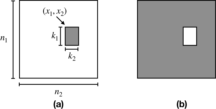
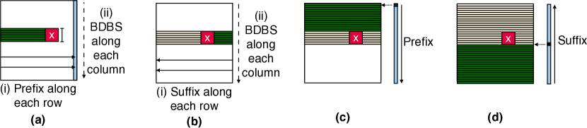
Although the excluded-sums problem is particularly challenging and meaningful for multidimensional tensors, let us start by considering the problem in only 2 dimensions. And, to understand the excluded-sums problem, it helps to understand the included-sums problem as well. Figure 1 illustrates included and excluded sums in 2 dimensions, and Figure 2 provides examples using ordinary addition as the operator. We have an matrix of elements over a monoid . We also are given a “box size” such that and . The included sum at a coordinate , as shown in Figure 1(a), involves reducing — accumulating using — all the elements of inside the -box cornered at , that is,
where if a coordinate goes out of range, we assume that its value is the identity . The included-sums problem computes the included sum for all coordinates of , which can be straightforwardly accomplished with four nested loops in time. Similarly, the excluded sum at a coordinate, as shown in Figure 1(b), reduces all the elements of outside the -box cornered at . The excluded-sums problem computes the excluded sum for all coordinates of , which can be straightforwardly accomplished in time. We shall see much better algorithms for both problems.
Excluded Sums and Operator Inverse
One way to solve the excluded-sums problem is to solve the included-sums problem and then use the inverse of the operator to “subtract” out the results from the reduction of the entire tensor. This approach fails for operators without inverse, however, such as the maximum operator . As another example, the FMM involves solving the excluded-sums problem over a domain of functions which cannot be “subtracted,” because the functions exhibit singularities [13]. Even for simpler domains, using the inverse (if it exists) may have unintended consequences. For example, subtracting finite-precision floating-point values can suffer from catastrophic cancellation [13, 30] and high round-off error [19]. Some contexts may permit the use of an inverse, but others may not.
Consequently, we refine the included- and excluded-sums problems into weak and strong versions. The weak version requires an operator inverse, while the strong version does not. Any algorithm for the included-sums problem trivially solves the weak excluded-sums problem, and any algorithm for the strong excluded-sums problem trivially solves the weak excluded-sums problem. This paper presents efficient algorithms for both the weak and strong excluded-sums problems.
Summed-area Table for Weak Excluded Sums
The summed-area table (SAT) algorithm uses the classical summed-area table method [11, 7, 29] to solve the weak included-sums problem on a -dimensional tensor having elements in time. This algorithm precomputes prefix sums along each dimension of and uses inclusion-exclusion to “add” and “subtract” prefixes to find the included sum for arbitrary boxes. The SAT algorithm cannot be used to solve the strong included-sums problem, however, because it requires an operator inverse. The summed-area table algorithm can easily be extended to an algorithm for weak excluded-sums by totaling the entire tensor and subtracting the solution to weak included sums. We will call this algorithm the SAT complement (SATC) algorithm.
Corners Algorithm for Strong Excluded Sums
The naive algorithm for strong excluded sums that just sums up the area of interest for each element runs in time in the worst case, because it wastes work by recomputing reductions for overlapping regions. To avoid recomputing sums, Demaine et al. [13] introduced an algorithm that solve the strong excluded-sums problem in arbitrary dimensions, which we will call the corners algorithm.
At a high level, the corners algorithm partitions the excluded region for each box into disjoint regions that each share a distinct vertex of the box, while collectively filling the entire tensor, excluding the box. The algorithm heavily depends on prefix and suffix sums to compute the reduction of elements in each of the disjoint regions.
Since the original article that proposed the corners algorithm does not include a formal analysis of its runtime or space usage in arbitrary dimensions, we present one in Appendix A. Given a -dimensional tensor of elements, the corners algorithm takes time to compute the excluded sum in the best case because there are corners and each one requires time to add its contribution to each excluded box. As we’ll see, the bound is tight: given space, the corners algorithm takes time. With space, the corners algorithm takes time.
| Source | Time | Space | Included or Excluded? | Strong or Weak? | |
| Naive included sum | [This work] | Included | Strong | ||
| Naive included sum complement | [This work] | Excluded | Weak | ||
| Naive excluded sums | [This work] | Excluded | Strong | ||
| Summed-area table (SAT) | [11, 29] | Included | Weak | ||
| [11, 29] | Excluded | Weak | |||
| Corners(c) | [13] | Excluded | Strong | ||
| Corners Spine(c) | [13] | Excluded | Strong | ||
| Bidirectional box sum (BDBS) | [This work] | Included | Strong | ||
| [This work] | Excluded | Weak | |||
| [This work] | Excluded | Strong |
Contributions
This paper presents algorithms for included and strong excluded sums in arbitrary dimensions that improve the runtime from exponential to linear in the number of dimensions. For strong included sums, we introduce the bidirectional box-sum (BDBS) algorithm that uses prefix and suffix sums to compute the included sum efficiently. The BDBS algorithm can be easily extended into an algorithm for weak excluded sums, which we will call the bidirectional box-sum complement (BDBSC) algorithm. For strong excluded sums, the main insight in this paper is the formulation of the excluded sums in terms of the “box complement” on which the box-complement algorithm is based. Table 1 summarizes all algorithms considered in this paper.
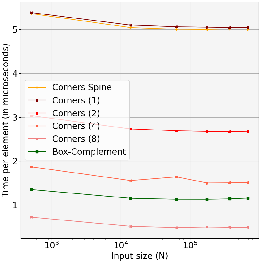
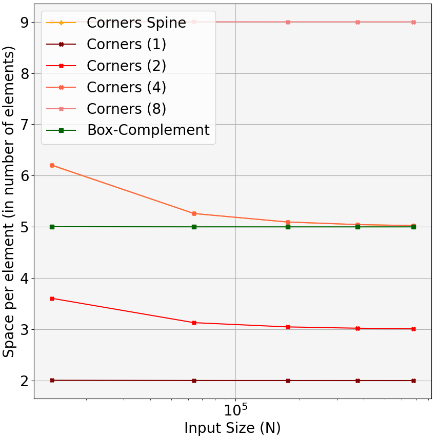
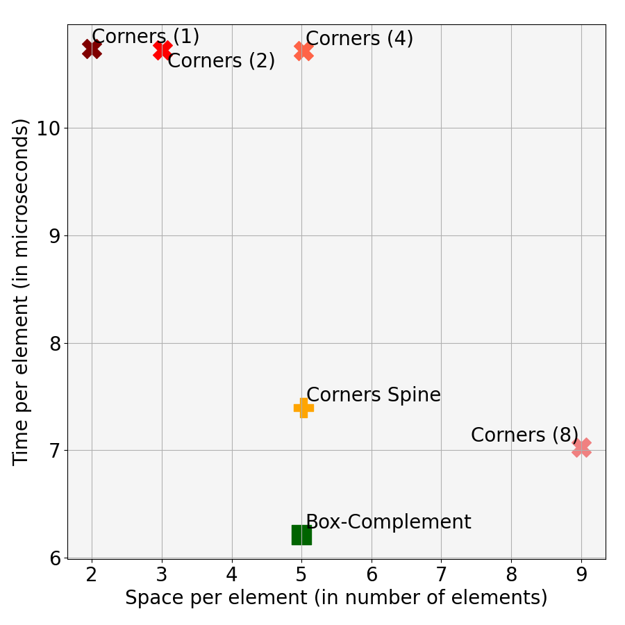
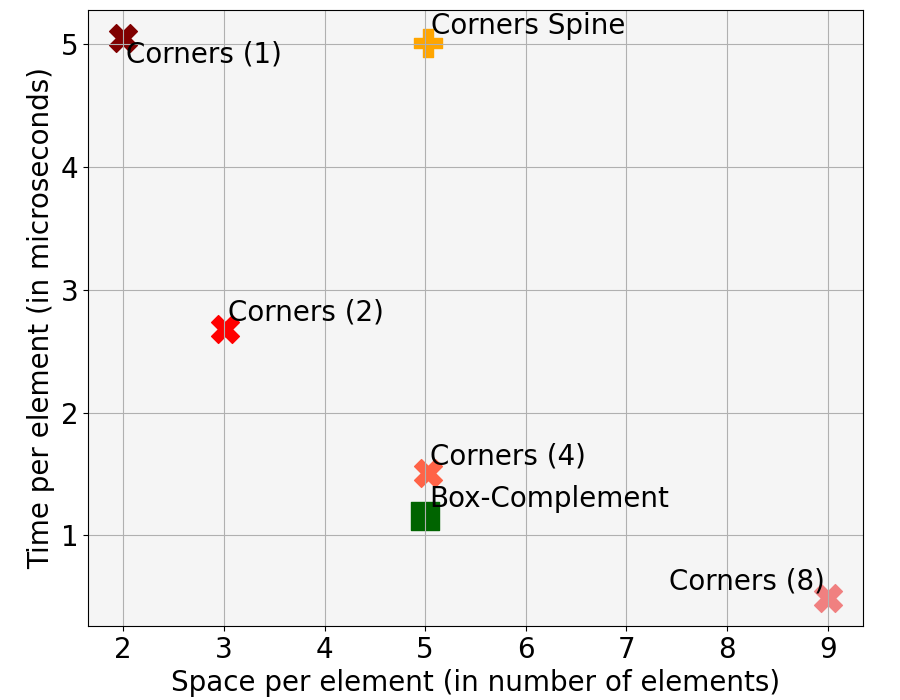
Figure 3 illustrates the performance and space usage of the box-complement algorithm and variants of the 3D corners algorithm. Since the paper that introduced the corners algorithm stopped short of a general construction in higher dimensions, the 3D case is the highest dimensionality for which we have implementations of the box-complement and corners algorithm. The 3D case is of interest because applications such as the FMM often present in three dimensions [17, 8]. We find that the box-complement algorithm outperforms the corners algorithm by about when given similar amounts of space, though the corners algorithm with twice the space as box-complement is faster. The box-complement algorithm uses a fixed (constant) factor of extra space, while the corners algorithm can use a variable amount of space. We found that the performance of the corners algorithm depends heavily on its space usage. We use Corners(c) to denote the implementation of the corners algorithm that uses a factor of in space to store leaves in the computation tree and gather the results into the output. Furthermore, we also explored a variant of the corners algorithm in Appendix A, called Corners Spine, which uses extra space to store the spine of the computation tree and asymptotically reduce the runtime.
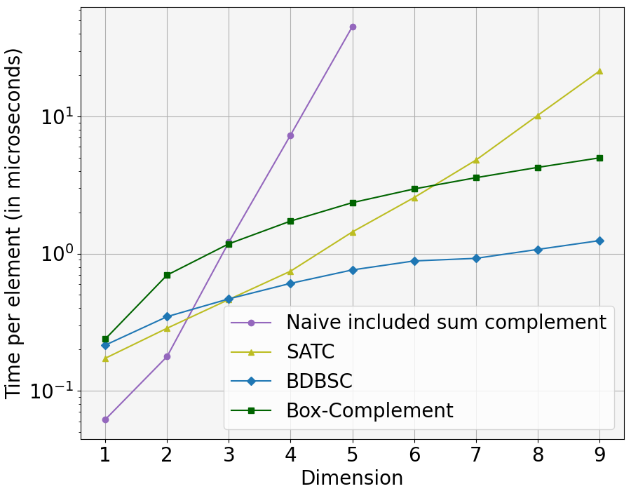
Figure 4 demonstrates how algorithms for weak excluded sums scale with dimension. We omit the corners algorithm because the original paper stopped short of a construction of how to find the corners in higher dimensions. We also omit an evaluation of included-sums algorithms because the relative performance of all algorithms would be the same. The naive and summed-area table perform well in lower dimensions but exhibit crossover points (at 3 and 6 dimensions, respectively) because their runtimes grow exponentially with dimension. In contrast, the BDBS and box-complement algorithms scale linearly in the number of dimensions and outperform the summed-area table method by at least after 6 dimensions. The BDBS algorithm demonstrates the advantage of solving the weak problem, if you can, because it is always faster than the box-complement algorithm, which doesn’t exploit an operator inverse. Both algorithms introduced in this paper outperform existing methods in higher dimensions, however.
To be specific, our contributions are as follows:
-
•
the bidirectional box-sum (BDBS) algorithm for strong included sums;
-
•
the bidirectional box-sum complement (BDBSC) algorithm for weak excluded sums;
-
•
the box-complement algorithm for strong excluded sums;
-
•
theorems showing that, for a -dimensional tensor of size , these algorithms all run in time and space;
-
•
implementations of these algorithms in C++; and
-
•
empirical evaluations showing that the box-complement algorithm outperforms the corners algorithm in 3D given similar space and that both the BDBSC algorithm and box-complement algorithm outperform the SATC algorithm in higher dimensions.
Outline
The rest of the paper is organized as follows. Section 2 provides necessary preliminaries and notation to understand the algorithms and proofs. Section 3 presents an efficient algorithm to solve the included-sums problem, which will be used as a key subroutine in the box-complement algorithm. Section 4 formulates the excluded sum as the “box-complement,” and Section 5 describes and analyzes the resulting box-complement algorithm. Section 6 presents an empirical evaluation of algorithms for excluded sums. Finally, we provide concluding remarks in Section 7.
2 Preliminaries
This section reviews tensor preliminaries used to describe algorithms in later sections. It also formalizes the included- and excluded-sums problems in terms of tensor notation. Finally, it describes the prefix- and suffix-sums primitive underlying the main algorithms in this paper.
Tensor Preliminaries
We first introduce the coordinate and tensor notation we use to explain our algorithms and why they work. At a high level, tensors are -dimensional arrays of elements over some monoid . In this paper, tensors are represented by capital script letters (e.g., ) and vectors are represented by lowercase boldface letters (e.g., ).
We shall use the following terminology. A -dimensional coordinate domain is is the cross product , where for . The size of is . Given a coordinate domain and a monoid as defined in Section 1, a tensor can be viewed for our purposes as a mapping . That is, a tensor maps a coordinate to an element . The size of a tensor is the size of its coordinate domain. We omit the coordinate domain and monoid when they are clear from context.
We use Python-like colon notation , where , to denote the half-open interval of coordinates along a particular dimension. If would extend outside of , where is the maximum coordinate, it denotes only the coordinates actually in the interval, that is, the interval . If the lower bound is missing, as in , we interpret the interval as , and similarly, if the upper bound is missing, as in , it denotes the interval . If both bounds are missing, as in , we interpret the interval as the whole coordinate range .
We can use colon notation when indexing a tensor to define subtensors, or boxes. For example, denotes the elements of at coordinates . For full generality, a box cornered at coordinates and , where for all , is the box . Given a box size , a -box cornered at coordinate is the box cornered at and . A (tensor) row is a box with a single value in each coordinate position in the colon notation, except for one position, which includes that entire dimension. For example, if is a coordinate of a tensor , then denotes a row along dimension .
The colon notation can be combined with the reduction operator to indicate the reduction of all elements in a subtensor:
Problem Definitions
We can now formalize the included- and excluded-sums problems from Section 1.
Definition 1 (Included and Excluded Sums)
An algorithm for the included-sums problem takes as input a -dimensional tensor with size and a box size . It produces a new tensor such that every output element holds the reduction under of elements within the -box of cornered at . An algorithm for the excluded-sums problem is defined similarly, except that the reduction is of elements outside the -box cornered at .
In other words, an included-sums algorithm computes, for all , the value . It’s messier to write the output of an excluded-sums problem using colon notation, but fortunately, our proofs do not rely on it.
As we have noted in Section 1, there are weak and strong versions of both problems which allow and do not allow an operator inverse, respectively.
Prefix and Suffix Sums
The prefix-sums operation [4] takes an array of elements and returns the “running sum” where
| (2.1) |
Let Prefix denote the algorithm that directly implements the recursion in Equation 2.1. Given an array and indices , the function Prefix computes the prefix sum in the range of in time. Similarly, the suffix-sums operation is the reverse of the prefix sum and computes the sum right-to-left rather than left-to-right. Let Suffix be the corresponding algorithm for suffix sums.
3 Included Sums
This section presents the bidirectional box-sum algorithm (BDBS) algorithm to compute the included sum along an arbitrary dimension, which is used as a main subroutine in the box-complement algorithm for excluded sums. As a warm-up, we will first describe how to solve the included-sums problem in one dimension and extend the technique to higher dimensions. We include the one-dimensional case for clarity, but the main focus of this paper is the multidimensional case.
We will sketch the subroutines for higher dimensions in this section. The full version of the paper includes all the pseudocode and omitted proofs for BDBS in 1D. We sketch the key subroutines in higher dimensions and omit them from this paper because they straightforwardly extend the computation from 1 dimension.
Included Sums in 1D
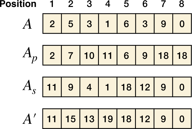
Before investigating the included sums in higher dimensions, let us first turn our attention to the 1D case for ease of understanding. Figure 13 presents an algorithm BDBS-1D which takes as input a list of length and a (scalar) box size111For simplicity in the algorithm descriptions and pseudocode, we assume that for all dimensions . In implementations, the input can either be padded with the identity to make this assumption hold, or it can add in extra code to deal with unaligned boxes. and outputs a list of corresponding included sums. At a high level, the BDBS-1D algorithm generates two intermediate lists and , each of length , and performs prefix and suffix sums of length on each intermediate list. By construction, for , we have , and .
Finally, BDBS-1D uses and to compute the included sum of size for each coordinate in one pass. Figure 5 illustrates the ranged prefix and suffix sums in BDBS-1D, and Figure 6 presents a concrete example of the computation.
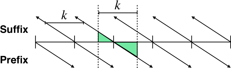
BDBS-1D solves the included-sums problem on an array of size in time and space. First, it uses two temporary arrays to compute the prefix and suffix as illustrated in Figure 5 in time. It then makes one more pass through the data to compute the included sum, requiring time. Figure 13 in Appendix B contains the full pseudocode for BDBS-1D.
Generalizing to Arbitrary Dimensions
The main focus of this work is multidimensional included and excluded sums. Computing the included sum along an arbitrary dimension is almost exactly the same as computing it along 1 dimension in terms of the underlying ranged prefix and suffix sums. We sketch an algorithm BDBS that generalizes BDBS-1D to arbitrary dimensions.
Let be a -dimensional tensor with elements and let be a box size. The BDBS algorithm computes the included sum along dimensions in turn. After performing the included-sum computation along dimensions , every coordinate in the output contains the included sum in each dimension up to :
Overall, BDBS computes the full included sum of a tensor with elements in time and space by performing the included sum along each dimension in turn.
Although we cannot directly use BDBS to solve the strong excluded-sums problem, the next sections demonstrate how to use the BDBS technique as a key subroutine in the box-complement algorithm for strong excluded sums.
4 Excluded Sums and the Box Complement
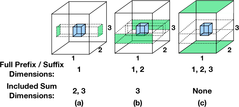
The main insight in this section is the formulation of the excluded sum as the recursive “box complement”. We show how to partition the excluded region into non-overlapping parts in dimensions. This decomposition of the excluded region underlies the box-complement for strong excluded sums in the next section.
First, let’s see how the formulation of the “box complement” relates to the excluded sum. At a high level, given a box , a coordinate is in the “-complement” of if and only if is “out of range” in some dimension , and “in the range” for all dimensions greater than .
Definition 2 (Box Complement)
Given a -dimensional coordinate domain and a dimension , the i-complement of a box cornered at coordinates and is the set
Given a box , the reduction of all elements at coordinates in is exactly the excluded sum with respect to . The box complement recursively partitions an excluded region into disjoint sets of coordinates.
Theorem 4.1 (Recursive Box-complement)
Let be a box cornered at coordinates and in some coordinate domain . The -complement of can be expressed recursively in terms of the -complement of as follows:
where .
-
Proof.
For simplicity of notation, let be the right-hand side of the equation in the statement of Theorem 4.1. Let be a coordinate. In order to show the equality, we will show that if and only if .
Forward Direction: .
We proceed by case analysis when . Let be the highest dimension at which is “out of range,” or where or .
Case 1: .
Definition 2 and imply that either
or , and for all
. By definition, implies
. Similarly, implies
. These are exactly the first two terms in .
Case 2: .
Definition 2 and
imply that .
Backwards Direction:
.
We again proceed by case analysis.
Case 1: .
Definition 2 implies
because there
exists some (in this case, ) such that and
for all .
Case 2: .
Definition 2 implies that there exists in the range such that
or and that for all
, we have . Therefore, implies
since there exists some (in this case,
) where or and
for all .
Therefore, can be recursively expressed as .
In general, unrolling the recursion in Theorem 4.1 yields disjoint partitions that exactly comprise the excluded sum with respect to a box.
Corollary 4.1 (Excluded-sum Components)
The excluded sum can be represented as the union of disjoint sets of coordinates as follows:
We use the box-complement formulation in the next section to efficiently compute the excluded sums on a tensor by reducing in disjoint regions of the tensor.
5 Box-Complement Algorithm
This section describes and analyzes the box-complement algorithm for strong excluded sums, which efficiently implements the dimension reduction in Section 4. The box-complement algorithm relies heavily on prefix, suffix, and included sums as described in Sections 2 and 3.
Given a -dimensional tensor of size and a box size , the box-complement algorithm solves the excluded-sums problem with respect to for coordinates in in time and space. Appendix C contains all omitted pseudocode and proofs for the serial box-complement algorithm.
Algorithm Sketch
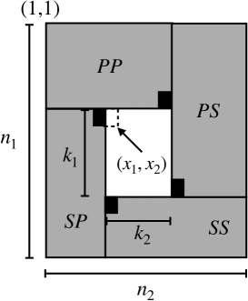
At a high level, the box-complement algorithm proceeds by dimension reduction. That is, the algorithm takes dimension-reduction steps, where each step adds two of the components from Corollary 4.1 to each element in the output tensor. In the th dimension-reduction step, the box-complement algorithm computes the -complement of (Definition 2) for all coordinates in the tensor by performing a prefix and suffix sum along the th dimension and then performing the BDBS technique along the remaining dimensions. After the th dimension-reduction step, the box-complement algorithm operates on a tensor of dimensions because dimensions have been reduced so far via prefix sums. Figure 7 presents an example of the dimension reduction in 2 dimensions, and Figure 8 illustrates the recursive box-complement in 3 dimensions.
Prefix and Suffix Sums
In the th dimension reduction step, the box-complement algorithm uses prefix and suffix sums along the th dimension to reduce the elements “out of range” along the th dimension in the -complement. That is, given a tensor of size and a number of dimensions reduced so far, we define a subroutine Prefix-Along-Dim that fixes the first dimensions at (respectively), and then computes the prefix sum along dimension for all remaining rows in dimensions . The pseudocode for Prefix-Along-Dim can be found in Figure 14 in Appendix C, and the proof that it incurs time can be found in Appendix C.
The subroutine Prefix-Along-Dim computes the reduction of elements “out of range” along dimension . That is, after Prefix-Along-Dim, for each coordinate along dimension , every coordinate in the (dimension-reduced) output contains the prefix up to that coordinate in dimension :
Since the similar subroutine Suffix-Along-Dim has almost exactly the same analysis and structure, we omit its discussion.
Included Sums
In the th dimension reduction step, the box-complement algorithm uses the BDBS technique along the th dimension to reduce the elements “in range” along the th dimension in the -complement. That is, given a tensor of size and a number of dimensions reduced so far, we define a subroutine BDBS-Along-Dim.
BDBS-Along-Dim computes the included sum for each row along a specified dimension after dimension reduction. Let be a -dimensional tensor, be a box size, be the number of reduced dimensions so far, and be the dimension to compute the included sum along such that . BDBS-Along-Dim computes the included sum along the th dimension for all rows . That is, for each coordinate , the output tensor contains the included sum along dimension :
BDBS-Along-Dim takes time because it iterates over rows and runs in time per row. It takes space using the same technique as BDBS-1D.
Adding in the Contribution
Each dimension-reduction step must add its respective contribution to each element in the output. Given an input tensor and output tensor , both of size , the function Add-Contribution takes time to add in the contribution with a pass through the tensors. The full pseudocode can be found in Figure 15 in Appendix C.
Putting It All Together
Finally, we will see how to use the previously defined subroutines to describe and analyze the box-complement algorithm for excluded sums. Figure 9 presents pseudocode for the box-complement algorithm. Each dimension-reduction step has a corresponding prefix and suffix step to add in the two components in the recursive box-complement. Given an input tensor of size , the box-complement algorithm takes space because all of its subroutines use at most a constant number of temporaries of size , as seen in Figure 9.
Given a tensor as input, the box-complement algorithm solves the excluded-sums problem by computing the recursive box-complement components from Corollary 4.1. By construction, for dimension , the prefix-sum part of the th dimension-reduction step outputs a tensor such that for all coordinates , we have
Similarly, the suffix-sum step constructs a tensor such that for all ,
We can now analyze the performance of the box-complement algorithm.
Theorem 5.1 (Time of Box-complement)
Given a -dimensional tensor of size , Box-Complement solves the excluded-sums problem in time.
-
Proof.
We analyze the prefix step (since the suffix step is symmetric, it has the same running time). Let denote a dimension.
The th dimension reduction step in Box-Complement involves 1 prefix step and () included sum calls, which each have time. Furthermore, adding in the contribution at each dimension-reduction step takes time. The total time over steps is therefore
Adding in the contribution is clearly in total.Next, we bound the runtime of the prefix and included sums. In each dimension-reduction step, reducing the number of dimensions of interest exponentially decreases the size of the considered tensor. That is, dimension reduction exponentially reduces the size of the input: . The total time required to compute the box-complement components is therefore
Therefore, the total time of Box-Complement is .
-
Box-Complement
1// Input: Tensor with -dimensions, box size // Output: Tensor with size and dimensions // matching containing the excluded sum. 2init with the same size as 3 4// Current dimension-reduction step 5for to 6// Saved from previous dimension-reduction step. 7 reduced up to dimension 8 // Save input to suffix step 9 // PREFIX STEP // Reduced up to dimensions. 10 Prefix-Along-Dim along 11 dimension on . 12 // Save for next round 13 // Do included sum on dimensions . 14 for to 15 // reduced up to dimensions 16 BDBS-Along-Dim on 17 dimension in 18 // Add into result 19 Add-Contribution from into 20 21 // SUFFIX STEP // Do suffix sum along dimension 22 Suffix-Along-Dim along 23 dimension in 24 // Do included sum on dimensions 25 for to 26 // reduced up to dimensions 27 BDBS-Along-Dim on 28 dimension in 29 // Add into result 30 Add-Contribution from into 31return
6 Experimental Evaluation
This section presents an empirical evaluation of strong and weak excluded-sums algorithms. In 3 dimensions, we compare strong excluded-sums algorithms: specifically, we evaluate the box-complement algorithm and variants of the corners algorithm and find that the box-complement outperforms the corners algorithm given similar space. Furthermore, we compare weak excluded-sums algorithms in higher dimensions. Lastly, to simulate a more expensive operator than numeric addition when reducing, we compare the box-complement algorithm and variants of the corners algorithm using an artificial slowdown.
Experimental Setup
We implemented all algorithms in C++. We used the Tapir/LLVM [27] branch of the LLVM[23, 24] compiler (version 9) with the -O3 and -march=native and -flto flags.
All experiments were run on a 8-core 2-way hyper-threaded Intel Xeon CPU E5-2666 v3 @ 2.90GHz with 30GB of memory from AWS [1]. For each test, we took the median of 3 trials.
To gather empirical data about space usage, we interposed malloc and free. The theoretical space usage of the different algorithms can be found in Table 1.
Strong Excluded Sums in 3D
Figure 3 summarizes the results of our evaluation of the box-complement and corners algorithm in 3 dimensions with a box length of (for a total box volume of ) and number of elements . We tested with varying but found that the time and space per element were flat (full results in Appendix D). We found that the box-complement algorithm outperforms the corners algorithm by about when given similar amounts of space, though the corners algorithm with the space as the box-complement algorithm was faster.
We explored two different methods of using extra space in the corners algorithm based on the computation tree of prefixes and suffixes: (1) storing the spine of the computation tree to asymptotically reduce the running time, and (2) storing the leaves of the computation tree to reduce passes through the output. Although storing the leaves does not asymptotically affect the behavior of the corners algorithm, we found that reducing the number of passes through the output has significant effects on empirical performance. Storing the spine did not improve performance, because the runtime is dominated by the number of passes through the output.
Excluded Sums With Different Operators
Most of our experiments used numeric addition for the operator. Because some applications, such as FMM, involve much more costly operators, we studied how the excluded-sum algorithms scale with the cost of . To do so, we added a tunable slowdown to the invocation of in the algorithms. Specifically, they call an unoptimized implementation of the standard recursive Fibonacci computation. By varying the argument to the Fibonacci function, we can simulate operators that take different amounts of time.
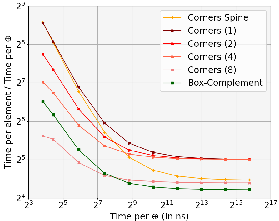
Figure 10 summarizes our findings. We ran the algorithms on a 3D domain of elements. (Although this domain may seem small, Appendix D shows that the results are relatively insensitive to domain size.) For inexpensive operators, the box-complement algorithm is the second fastest, but as the cost of increases, the box-complement algorithm dominates. The reason for this outcome is that box-complement performs approximately operations per element in 3D, whereas the most efficient corners algorithm performs about operations. As becomes more costly, the time spent executing dominates the other bookkeeping overhead.
Weak Excluded Sums in Higher Dimensions
Figure 4 presents the results of our evaluation of weak excluded-sum algorithms in higher dimensions. For all dimensions , we set the box length and chose a number of elements to be a perfect power of dimension . Table 1 presents the asymptotic runtime of the different excluded-sum algorithms.
The weak naive algorithm for excluded sums with nested loops outperforms all of the other algorithms up to 2 dimensions because its runtime is dependent on the box volume, which is low in smaller dimensions. Since its runtime grows exponentially with the box length, however, we limited it to 5 dimensions.
The summed-area table algorithm outperforms the BDBS and box-complement algorithms up to 6 dimensions, but its runtime scales exponentially in the number of dimensions.
Finally, the BDBS and box-complement algorithms scale linearly in the number of dimensions and outperform both naive and summed-area table methods in higher dimensions. Specifically, the box-complement algorithm outperforms the summed-area table algorithm by between and after 6 dimensions. The BDBS algorithm demonstrates an advantage to having an inverse: it outperforms the box-complement algorithm by to . Therefore, the BDBS algorithm dominates the box-complement algorithm for weak excluded sums.
7 Conclusion
In this paper, we introduced the box-complement algorithm for the excluded-sums problem, which improves the running time of the state-of-the-art corners algorithm from to time. The space usage of the box-complement algorithm is independent of the number of dimensions, while the corners algorithm may use space dependent on the number of dimensions to achieve its running-time lower bound.
The three new algorithms from this paper parallelize straightforwardly. In the work/span model [10], all three algorithms are work-efficient, achieving work. The BDBS and BDBSC algorithms achieve span, and the box-complement algorithm achieves span.
Acknowledgments
The idea behind the box-complement algorithm was originally conceived jointly with Erik Demaine many years ago, and we thank him for helpful discussions. Research was sponsored by the United States Air Force Research Laboratory and the United States Air Force Artificial Intelligence Accelerator and was accomplished under Cooperative Agreement Number FA8750-19-2-1000. The views and conclusions contained in this document are those of the authors and should not be interpreted as representing the official policies, either expressed or implied, of the United States Air Force or the U.S. Government. The U.S. Government is authorized to reproduce and distribute reprints for Government purposes notwithstanding any copyright notation herein.
References
- [1] Amazon. Amazon Web Services. https://aws.amazon.com/, 2021.
- [2] Rick Beatson and Leslie Greengard. A short course on fast multipole methods. Wavelets, Multilevel Methods and Elliptic PDEs, pages 1–37, 1997.
- [3] Pierre Blanchard, Nicholas J. Higham, and Theo Mary. A class of fast and accurate summation algorithms. SIAM Journal on Scientific Computing, 42(3):A1541–A1557, 2020.
- [4] Guy E. Blelloch. Prefix sums and their applications. Technical Report CMU-CS-90-190, School of Computer Science, Carnegie Mellon University, November 1990.
- [5] Guy E. Blelloch, Daniel Anderson, and Laxman Dhulipala. ParlayLib: a toolkit for parallel algorithms on shared-memory multicore machines. page 507–509, 2020.
- [6] Robert D. Blumofe, Christopher F. Joerg, Bradley C. Kuszmaul, Charles E. Leiserson, Keith H. Randall, and Yuli Zhou. Cilk: An efficient multithreaded runtime system. Journal of Parallel and Distributed Computing, 37(1):55–69, 1996.
- [7] Derek Bradley and Gerhard Roth. Adaptive thresholding using the integral image. Journal of Graphics Tools, 12(2):13–21, 2007.
- [8] Hongwei Cheng, William Y. Crutchfield, Zydrunas Gimbutas, Leslie F. Greengard, J. Frank Ethridge, Jingfang Huang, Vladimir Rokhlin, Norman Yarvin, and Junsheng Zhao. A wideband fast multipole method for the Helmholtz equation in three dimensions. Journal of Computational Physics, 216(1):300–325, 2006.
- [9] Ronald Coifman, Vladimir Rokhlin, and Stephen Wandzura. The fast multipole method for the wave equation: A pedestrian prescription. IEEE Antennas and Propagation Magazine, 35(3):7–12, 1993.
- [10] Thomas H. Cormen, Charles E. Leiserson, Ronald L. Rivest, and Clifford Stein. Introduction to Algorithms. MIT Press, 3rd edition, 2009.
- [11] Franklin C. Crow. Summed-area tables for texture mapping. pages 207–212, 1984.
- [12] Eric Darve. The fast multipole method: numerical implementation. Journal of Computational Physics, 160(1):195–240, 2000.
- [13] E. D. Demaine, M. L. Demaine, A. Edelman, C. E. Leiserson, and P. Persson. Building blocks and excluded sums. SIAM News, 38(4):1–5, 2005.
- [14] S. Fraser, H. Xu, and C. E. Leiserson. Work-efficient parallel algorithms for accurate floating-point prefix sums. In 2020 IEEE High Performance Extreme Computing Conference (HPEC), pages 1–7, 2020.
- [15] Sean Fraser. Computing included and excluded sums using parallel prefix. Master’s thesis, Massachusetts Institute of Technology, 2020.
- [16] L. Greengard and V. Rokhlin. A fast algorithm for particle simulations. J. Comput. Phys., 135(2):280–292, August 1997.
- [17] Nail A. Gumerov and Ramani Duraiswami. Fast multipole methods for the Helmholtz equation in three dimensions. Elsevier, 2005.
- [18] Justin Hensley, Thorsten Scheuermann, Greg Coombe, Montek Singh, and Anselmo Lastra. Fast summed-area table generation and its applications. In Computer Graphics Forum, volume 24, pages 547–555. Wiley Online Library, 2005.
- [19] Nicholas J. Higham. The accuracy of floating point summation. SIAM J. Scientific Computing, 14:783–799, 1993.
- [20] Nicholas J. Higham. Accuracy and Stability of Numerical Algorithms. Society for Industrial and Applied Mathematics, Philadelphia, PA, USA, 2nd edition, 2002.
- [21] Intel Corporation. Intel Cilk Plus Language Specification, 2010. Document Number: 324396-001US. Available from http://software.intel.com/sites/products/cilk-plus/cilk_plus_language_specification.pdf.
- [22] Peter M. Kogge and Harold S. Stone. A parallel algorithm for the efficient solution of a general class of recurrence equations. IEEE Transactions on Computers, 100(8):786–793, 1973.
- [23] Chris Lattner. LLVM: An infrastructure for multi-stage optimization. Master’s thesis, Computer Science Dept., University of Illinois at Urbana-Champaign, Urbana, IL, December 2002.
- [24] Chris Lattner and Vikram Adve. LLVM: A compilation framework for lifelong program analysis & transformation. In International Symposium on Code Generation and Optimization (CGO), page 75, Palo Alto, California, March 2004.
- [25] William B March and George Biros. Far-field compression for fast kernel summation methods in high dimensions. Applied and Computational Harmonic Analysis, 43(1):39–75, 2017.
- [26] Tao B. Schardl, William S. Moses, and Charles E. Leiserson. Tapir: Embedding fork-join parallelism into LLVM’s intermediate representation. In ACM SIGPLAN Notices, volume 52, pages 249–265. ACM, 2017.
- [27] Tao B Schardl, William S Moses, and Charles E Leiserson. Tapir: Embedding recursive fork-join parallelism into llvm’s intermediate representation. ACM Transactions on Parallel Computing (TOPC), 6(4):1–33, 2019.
- [28] Xiaobai Sun and Nikos P Pitsianis. A matrix version of the fast multipole method. Siam Review, 43(2):289–300, 2001.
- [29] Ernesto Tapia. A note on the computation of high-dimensional integral images. Pattern Recognition Letters, 32(2):197–201, 2011.
- [30] Gernot Ziegler. Summed area computation using ripmap of partial sums, 2012. GPU Technology Conference (talk).
A Analysis of Corners Algorithm
This section presents an analysis of the time and space usage of the corners algorithm [13] for the excluded-sums problem. The original article that proposed the corners algorithm did not include an analysis of its performance. As we will see, the runtime of the corners algorithm is a function of the space it is allowed.
Algorithm Description.
Given a -dimensional tensor of size and a box , the corners algorithm partitions the excluded region into disjoint regions corresponding to the corners of the box. Each excluded sum is the sum of the reductions of each of the corresponding regions. The corners algorithm computes the reduction of each partition with a combination of prefix and suffix sums over the entire tensor and saves work by reusing prefixes and suffixes in overlapping regions. Figure 11 illustrates an example of the corners algorithm.
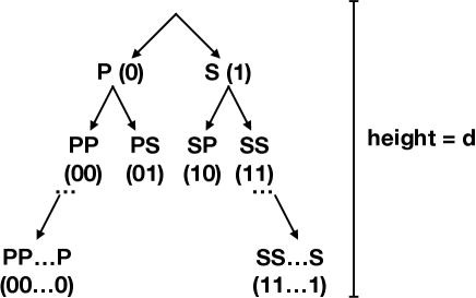
We can represent each length- combination of prefixes and suffixes as a length- binary string where a or in the -th position corresponds to a prefix or suffix (resp.) at depth . As illustrated in Figure 12, the corners algorithm defines a computation tree where each node represents a combination of prefixes and suffixes, and each edge from depth to represents a full prefix or suffix along dimension . The total height of this computation tree is , so there are leaves.
Analysis.
The most naive implementation of the corners algorithm that computes every root-to-leaf path without reusing computation between paths takes space, but time per leaf, for total time . We will see how to use extra space to reuse computation between paths and reduce the total time.
Theorem A.1 (Time / Space Tradeoff)
Given a multiplicative space allowance such that , the corners algorithm solves the excluded-sums problem in time if it is allowed space.
-
Proof.
The corners algorithm must traverse the entire computation tree in order to compute all of the leaves. If it follows a depth-first traversal of the tree, one possible use of the extra allowed space is to keep the intermediate combination of prefix and suffices at the first internal nodes along the current root-to-leaf path in the traversal. We will analyze this scheme in terms of 1) the amount of time that each leaf requires independently, and 2) the total shared work between leaves. The total time of the algorithm is the sum of these two components.
Independent work: For each leaf, if the first prefixes and suffixes have been computed along its root-to-leaf path, there are an additional prefix and suffix computations required to compute that leaf. Therefore, each leaf takes additional time outside of the shared computation, for a total of time.
Shared work: The remaining time of the algorithm is the amount of time it takes to compute the higher levels of the tree up to depth given a factor in space. Given a node at depth with position such that , the amount of time it takes to compute the intermediate sums along the root-to-leaf path to depends on the difference in the bit representation between and . Specifically, if and differ in bits, it takes additional time to store the intermediate sums for node at depth . In general, the number of nodes that differ in positions at depth is . Therefore, the total time of computing the intermediate sums isPutting it together: Each leaf also requires time to add in the contribution. Therefore, the total time is
The time of the corners algorithm is lower bounded by and minimized when . Given space, the corners algorithm solves the excluded-sums problem in time. Given space, the corners algorithm solves the excluded-sums problem in time.
B Included Sums Appendix
-
BDBS-1D
1// Input: List of size and // included-sum length . // Output: List of size where each // entry for . 2allocate with slots 3 4for to 5 // -wise prefix sum along 6 Prefix(, , ) 7 // -wise suffix sum along 8 Suffix(, , ) 9for to // Combine into result 10 if 11 12 else 13 14return
Lemma B.1 (Correctness in 1D)
BDBS-1D solves the included sums problem in 1 dimension.
-
Proof.
Consider a list with elements and box length . We will show that for each , the output contains the desired sum. For , this holds by construction. For all other , the previously defined prefix and suffix sum give the desired result. Recall that , and Also note that for all , .
Therefore,
which is exactly the desired sum.
Lemma B.2 (Time and Space in 1D)
Given an input array of size and box length , BDBS-1D takes time and space.
-
Proof.
The total time of the prefix and suffix sums is , and the loop that aggregates the result into has iterations of time each. Therefore, the total time of BDBS-1D is . Furthermore, BDBS-1D uses two temporary arrays of size each for the prefix and suffix, for total space .
C Excluded Sums Appendix
-
Prefix-Along-Dim
1// Input: Tensor ( dimensions, side lengths // (), dimension to do the prefix sum // along. // Output: Modify to do the prefix sum along // dimension , fixing dimensions up to . 2// Iterate through coordinates by varying // coordinates in dimensions // while fixing the first dimensions. // Blanks mean they are not iterated over // in the outer loop 3for 4 5 // Prefix sum along row // (can be replaced with a parallel prefix) 6 for to 7 8
The suffix sum along a dimension is almost exactly the same, so we omit it.
Lemma C.1 (Time of Prefix Sum)
Prefix-Along-Dim takes time.
-
Proof.
The outer loop over dimensions has iterations, each with work for the inner prefix sum. Therefore, the total time is .
-
Add-Contribution
1// Input: Input tensor , output tensor , // fixing dimensions up to . // Output: For all coords in , add the // relevant contribution from . 2for 3 if 4 5
Lemma C.2 (Adding Contribution)
Add-Contribution takes time.
-
1// Input: Tensor of dimensions and side lengths // output tensor , side lengths of the // excluded box , for all // . // Output: Tensor with size and dimensions // matching containing the excluded sum. 2 // Prefix and suffix temp 3for to // Current dimension-reduction step 4 // PREFIX STEP // At this point, should hold prefixes up to // dimension . 5 6 // Save the input to the suffix step 7 8 // Do prefix sum along dimension 9 Prefix-Along-Dim 10 // Save prefix up to dimension in 11 12 // Do included sum on dimensions 13 for to 14 BDBS-Along-Dim 15 // Add into result 16 Add-Contribution 17 // SUFFIX STEP // Start with the prefix up until dimension // 18 19 // Do suffix sum along dimension 20 Suffix-Along-Dim 21 // Do included sum on dimensions 22 for to 23 BDBS-Along-Dim 24 // Add into result 25 Add-Contribution
D Additional experimental data
The data in this appendix was generated with the experimental setup described in Section 6.