Control Occupation Kernel Regression for Nonlinear Control-Affine Systems

Abstract

This manuscript presents an algorithm for obtaining an approximation of nonlinear high order control affine dynamical systems, that leverages the controlled trajectories as the central unit of information. As the fundamental basis elements leveraged in approximation, higher order control occupation kernels represent iterated integration after multiplication by a given controller in a vector valued reproducing kernel Hilbert space. In a regularized regression setting, the unique optimizer for a particular optimization problem is expressed as a linear combination of these occupation kernels, which converts an infinite dimensional optimization problem to a finite dimensional optimization problem through the representer theorem. Interestingly, the vector valued structure of the Hilbert space allows for simultaneous approximation of the drift and control effectiveness components of the control affine system. Several experiments are performed to demonstrate the effectiveness of the approach.

1 Introduction

Consider a dynamical system, $\dot{x}=f(x)$, for unknown dynamics, $f:\mathbb{R}^{n}\to\mathbb{R}^{n}$. Given an observed trajectory, $\gamma:[0,T]\to\mathbb{R}^{n}$ satisfying the dynamics, system identification routines for dynamical systems have traditionally relied on taking numerical derivatives of observed trajectory data to determine samples for the dynamics [1]. However, numerical derivatives are sensitive to signal noise, where an addition of white noise can cause unbounded disturbances for numerical differentiation. Methods such as the SINDy algorithm [2, 3] ameliorate this issue through a total variation regularization, but even these methods have limitations with the respect to noise.

Recently, a collection of results surrounding the concept of occupation kernels have appeared, where system identification problems are addressed not through numerical differentiation, but rather through integration [4]. The integration approach is considerably less sensitive to signal noise, and can be incorporated in system identification routines naturally through reproducing kernel Hilbert spaces (RKHSs). Specifically, given a RKHS, $H$, of continuously differentiable functions (or simply continuous, depending on the context), the occupation kernel corresponding to $\gamma$ is the unique function that satisfies $\langle h,\Gamma_{\gamma}\rangle_{H}=\int_{0}^{T}h(\gamma(t))dt$. Moreover, if the components of the dynamics reside in the RKHS, $f=(f_{1},\ldots,f_{n})^{T}\in H^{n}$, then $\langle f_{i},\Gamma_{\gamma}\rangle_{H}=\int_{0}^{T}f_{i}(\gamma(t))dt=\int_{0}^{T}(\dot{\gamma}(t))_{i}dt=(\gamma(T)-\gamma(0))_{i}$ for each $i=1,\ldots,n$ (see [4]).

Occupation kernels generalize occupation measures, which have been leveraged extensively in optimal control, in a way analogous to how kernel functions generalize delta distributions [5, 6, 7]. In particular, like kernel functions, occupation kernels provide a function theoretic analog of their respective measures in a RKHS. Hence, occupation kernels themselves can be leveraged as basis functions for approximation, and indeed occupation kernels have been used in precisely that manner for motion tomography in [8] as well as for a regression approach to fractional order nonlinear system identification in [9]. Occupation kernels are also leveraged as basis functions for the construction of eigenfunctions for finite rank representations of Liouville operators in a continuous time Dynamic Mode Decomposition routine in [10].

The present manuscript generalizes two different approaches to system identification using occupation kernels, where occupation kernels for higher order control affine systems are introduced in Section 3, and these are leveraged as basis functions for the resolution of a regularized regression problem for higher order control affine systems of the form $\frac{d^{s}}{dt^{s}}x=f(x)+g(x)u$. Specifically, this extends the regression approach for fractional order dynamical systems in [9] as well as giving a generalization of the control occupation kernels used in combination with control Liouville operators in [11].

System identification using the new occupation kernels is realized through a regularized regression formulation, where the regularization forces the minimizer to be a linear combination of the occupation kernels, and in turn, leads to a finite dimensional optimization problem resolved by a matrix equation given in Section 4.

2 Problem Statement

The objective of this manuscript is to learn an unknown higher order control affine system from observed integrable controllers and controlled trajectories, $\{u_{j}:[0,T_{j}]\to\mathbb{R}^{m}\}_{i=1}^{M}$ and $\{\gamma_{u_{j}}:[0,T_{j}]\to\mathbb{R}^{n}\}_{j=1}^{M}$, respectively, satisfying

$$\frac{d^{s}}{dt^{s}}\gamma_{u_{j}}(t)=f(\gamma_{u_{j}}(t))+g(\gamma_{u_{j}}(t))u_{j}(t)$$ (1)

where $f:\mathbb{R}^{n}\to\mathbb{R}^{n}$ is the drift function, $g:\mathbb{R}^{n}\to\mathbb{R}^{n\times m}$ is the control effectiveness matrix, and $s\in\mathbb{N}$.

For several selections of $f$, $g$, and $s$, the formulation in (1) specializes to several different system identification problems. When $g\equiv 0$, the problem reduces to determining the unknown dynamics $f$ for a higher order dynamical system. When $s=1$ the problem becomes a system identification problem for a first order control-affine system. If $s=1$ and $g\equiv 0$, the method developed in this manuscript agrees with that of [9] for the case of $q=1$.

Systems of the form (1) encompass $s-$th order linear systems and Euler-Lagrange models with invertible inertia matrices, and hence, represent a wide class of physical plants, including but not limited to robotic manipulators and autonomous ground, aerial, and underwater vehicles.

3 Reproducing Kernels and Occupation Kernels

Given a Hilbert space $\mathcal{Y}$ and a set $X$, a vector valued RKHS, $H$, is a Hilbert space of functions from $X$ to $\mathcal{Y}$, such that for each $v\in\mathcal{Y}$ and $x\in X$, the functional $f\mapsto\langle f(x),v\rangle_{\mathcal{Y}}$ is bounded. Hence for each $x\in X$ and $v\in\mathcal{Y}$, there is a function $K_{x,v}\in H$ such that $\langle f(x),v\rangle_{\mathcal{Y}}=\langle f,K_{x,v}\rangle_{H}$. The mapping $v\mapsto K_{x,v}$ is linear over $\mathcal{Y}$; hence, $K_{x,v}$ may be expressed as an operator over $\mathcal{Y}$ as $K_{x}v:=K_{x,v}$. The operator $K(x,y):=K_{y}^{*}K_{x}$ is called the kernel operator corresponding to $H$.

In the present context, $\mathcal{Y}=\mathbb{R}^{m+1}$ (viewed as row vectors), $X=\mathbb{R}^{n}$, and $H$ consists of continuously differentiable functions. In this context, the operation on $v$ by the kernel will be expressed as $vK_{x}$. Given two continuous signals, $\theta:[0,T]\to\mathbb{R}^{n}$ and $u:[0,T]\to\mathbb{R}^{m}$, the control occupation kernel corresponding to this pair of signals is the unique function, $\Gamma_{\theta,u}\in H$, that represents the bounded functional $h\mapsto\int_{0}^{T}h(\theta(t))\begin{pmatrix}1\\ u(t)\end{pmatrix}dt=\langle h,\Gamma_{\theta,u}\rangle_{H}.$ Control occupation kernels were introduced in [11], and may be generalized for higher order dynamical systems through the Cauchy iterated integral formula.

Definition 1.

For a given continuous signal $\theta:[0,T]\to\mathbb{R}^{n}$, and vector valued RKHS as above, the control occupation kernel of order $s\in\mathbb{N}$ corresponding to $\theta$, $\Gamma_{\theta,u}^{(s)}$, in $H$ is given as the unique function that represents the bounded functional

$$\frac{1}{(s-1)!}\int_{0}^{T}(T-t)^{s-1}h(\theta(t))\begin{pmatrix}1\\ u(t)\end{pmatrix}dt=\langle h,\Gamma_{\theta,u}^{(s)}\rangle_{H}.$$

This definition enables the treatment of particular higher order dynamical systems without state augmentation. To wit, if $\gamma:[0,T]\to\mathbb{R}^{n}$ is a trajectory satisfying $\ddot{\gamma}=f(\gamma)$ for $f(\gamma)=(f_{1}(\gamma),f_{2}(\gamma),\ldots,f_{n}(\gamma))^{T}\in\mathbb{R}^{n}$ (taking for the moment $m=0$), then for each $j=1,\ldots,n$,

$$\langle f_{j},\Gamma_{\gamma,0}^{(2)}\rangle_{H}=(\gamma(T)-\gamma(0)-T\dot{\gamma}(0))_{j},$$

where the notation $(\cdot)_{j}$ indicates the $j$-th dimensional component of a vector. More generally, if $\gamma_{u}:[0,T]\to\mathbb{R}^{n}$ is a controlled trajectory (with controller $u:[0,T]\to\mathbb{R}^{m}$ corresponding to the control affine system $\ddot{\gamma}=f(\gamma)+g(\gamma)u$, where $g(\gamma)=(g_{1}^{T}(\gamma),\ldots,g_{n}^{T}(\gamma))^{T}\in\mathbb{R}^{n\times m}$, then

$$\langle\begin{pmatrix}f_{j}&g_{j}\end{pmatrix},\Gamma_{\gamma_{u},u}^{(2)}\rangle_{H}=(\gamma_{u}(T)-\gamma_{u}(0)-T\dot{\gamma}_{u}(0))_{j}.$$

More generally, the following proposition holds.

Proposition 1.

Suppose that $H$ is a vector valued RKHS consisting of $\mathbb{R}^{m+1}$ (row) valued continuous functions over $\mathbb{R}^{n}$. Let $\gamma_{u}:[0,T]\to\mathbb{R}^{n}$ be a controlled trajectory with continuous controller $u:[0,T]\to\mathbb{R}^{m}$ satisfying, for all $t\in[0,T]$, $\frac{d^{s}}{dt^{s}}\gamma(t)=f(\gamma(t))+g(\gamma(t))$ for $f=(f_{1},\ldots,f_{n})^{T}$ and $g=(g_{1}^{T},\ldots,g_{n}^{T})$ with $\begin{pmatrix}f_{j}&g_{j}\end{pmatrix}\in H$ for each $j=1,\ldots,n$. In this setting,

$$\langle\begin{pmatrix}f_{j}&g_{j}\end{pmatrix},\Gamma^{(s)}_{\theta_{u},u}\rangle_{H}=\left(\gamma_{u}(T)-\sum_{\ell=0}^{s-1}\frac{T^{\ell}}{\ell!}\frac{d^{\ell}}{dt^{\ell}}\gamma_{u}(0)\right)_{j}.$$

Proof.

Since $\begin{pmatrix}f_{j}(\gamma_{u}(t))&g_{j}(\gamma_{u}(t))\end{pmatrix}\begin{pmatrix}1\\ u(t)\end{pmatrix}=f_{j}(\gamma_{u}(t))+g_{j}(\gamma_{u}(t))u(t)=\frac{d^{s}}{dt^{s}}(\gamma_{u}(t))_{j}$, and $\Gamma_{\gamma_{u},u}^{(s)}$ implements Cauchy’s iterated integral formula through the inner product of the Hilbert space, the result follows through iterated applications of the fundamental theorem of calculus. ∎

While Proposition 1 follows from a simple application of the fundamental theorem of calculus, it sets the stage for a powerful approximation routine leveraging higher order control occupation kernels. These kernels can be implemented directly using a direct interpolation approach, or they can arise naturally in a regularized regression problem.

Section 4 explores a regularized regression approach for learning higher order control affine dynamical systems, where the dynamics may be expressed as a linear combination of higher order control occupation kernels. Therefore, it is necessary to have a cogent method for evaluating the higher order control occupation kernels, and this may be realized through inner products with the kernels $e_{j}K_{x}$, where $e_{j}$ is the $j$-th cardinal basis function for $\mathbb{R}^{m+1}$.

Proposition 2.

Fix $s\in\mathbb{N}$. Let $\theta$ and $u$ be continuous signals from $[0,T]$ to $\mathbb{R}^{n}$ and $\mathbb{R}^{m}$ respectively. Let $H$ be a vector valued RKHS as above, then

$$\Gamma^{(s)}_{\theta,u}(x)=\frac{1}{(s-1)!}\int_{0}^{T}(T-t)^{s-1}\begin{pmatrix}1&u^{T}(t)\end{pmatrix}^{T}K_{\theta(t)}(x)dt.$$ (2)

Proof.

Consider $\langle\Gamma^{(s)}_{\theta,u}(x),v\rangle_{\mathcal{Y}}=\langle\Gamma^{(s)}_{\theta,u},vK_{x}\rangle_{H},$ which follow from the definition of a vector valued RKHS. Symmetrically, since $H$ is a real valued RKHS, it follows that

$$\langle\Gamma^{(s)}_{\theta,u}(x),v\rangle_{\mathcal{Y}}=\langle\Gamma^{(s)}_{\theta,u},vK_{x}\rangle_{H}=\langle vK_{x},\Gamma^{(s)}_{\theta,u}\rangle_{H}=\frac{1}{(s-1)!}\int_{0}^{T}(T-t)^{s-1}vK_{x}(\theta(t))\begin{pmatrix}1\\ u(t)\end{pmatrix}dt$$

$$=\left\langle\frac{1}{(s-1)!}\int_{0}^{T}(T-t)^{s-1}\begin{pmatrix}1&u(t)^{T}\end{pmatrix}^{T}K_{\theta(t)}(x)dt,v\right\rangle_{\mathbb{R}^{m+1}}.$$

Hence, the equality holds for all $v\in\mathbb{R}^{m+1},$ and the result follows. ∎

4 A Regression Method using Control Occupation Kernels for Control Affine Systems

The learning approach adopted in this manuscript surrounds a regularized regression problem posed over a vector valued RKHS, $H$. Through the representer theorem, we will demonstrate that higher order control occupation kernels arise naturally as a collection of basis functions for approximating the control affine dynamics.

Given $\lambda>0$ and the controllers and controlled trajectories from Section 2, the regularized regresssion problem to determine an approximation of the $i$-th row of $f$ and $g$ within the vector valued RKHS is given as

$$\min_{\begin{pmatrix}\hat{f}_{i}&\hat{g}_{i}\end{pmatrix}\in H}\frac{1}{(s-1)!}\sum_{j=1}^{\infty}\left[\int_{0}^{T_{j}}(T_{j}-t)^{s-1}\left(\hat{f}_{i}(\gamma_{u_{j}}(t))+\hat{g}_{i}(\gamma_{u_{j}}(t))u_{j}(t)\right)dt-\right.$$

$$\left.\left(\gamma_{u_{j}}(T_{j})-\sum_{\ell=1}^{s-1}\frac{T_{j}^{\ell}}{\ell!}\frac{d^{\ell}}{dt^{\ell}}\gamma_{u_{j}}(0)\right)_{i}\right]+\lambda\|\begin{pmatrix}\hat{f}_{i}&\hat{g}_{i}\end{pmatrix}\|^{2}_{H}.$$ (3)

Through the representer theorem [12], the minimizer of (3) may be expressed as a linear combination of the higher order occupation kernels, $w_{1,i}\Gamma_{\gamma_{u_{1}},u_{1}}^{(s)}+\cdots+w_{M,i}\Gamma^{(s)}_{\gamma_{u_{M}},u_{M}}$. Hence, the resolution (3) reduces to a finite dimensional optimization problem, and ultimately the resolution of the linear system

$$\left(\begin{pmatrix}\langle\Gamma^{(s)}_{\gamma_{u_{1}},u_{1}},\Gamma^{(s)}_{\gamma_{u_{1}},u_{1}}\rangle_{H}&\cdots&\langle\Gamma^{(s)}_{\gamma_{u_{1}},u_{1}},\Gamma^{(s)}_{\gamma_{u_{M}},u_{M}}\rangle_{H}\\ \vdots&\ddots&\vdots\\ \langle\Gamma^{(s)}_{\gamma_{u_{1}},u_{1}},\Gamma^{(s)}_{\gamma_{u_{1}},u_{1}}\rangle_{H}&\cdots&\langle\Gamma^{(s)}_{\gamma_{u_{1}},u_{1}},\Gamma^{(s)}_{\gamma_{u_{M}},u_{M}}\rangle_{H}\end{pmatrix}+\lambda I_{M}\right)\begin{pmatrix}w_{1,1}&\cdots&w_{1,n}\\ \vdots\\ w_{M,1}&\cdots&w_{M,n}\end{pmatrix}$$

$$=\begin{pmatrix}\left(\gamma_{u_{1}}(T_{1})-\sum_{\ell=1}^{s-1}\frac{T_{1}^{\ell}}{\ell!}\frac{d^{\ell}}{dt^{\ell}}\gamma_{u_{1}}(0)\right)^{T}\\ \vdots\\ \left(\gamma_{u_{M}}(T_{M})-\sum_{\ell=1}^{s-1}\frac{T_{M}^{\ell}}{\ell!}\frac{d^{\ell}}{dt^{\ell}}\gamma_{u_{M}}(0)\right)^{T}\end{pmatrix}.$$ (4)

The resultant approximation is given as $\begin{pmatrix}f(x)&g(x)\end{pmatrix}=\sum_{j=1}^{M}\mathbb{w}_{j}\Gamma^{(s)}_{\gamma_{u_{j}},u_{j}}(x)$ where each $\mathbb{w}_{j}:=\begin{pmatrix}w_{j,1}&\ldots&w_{j,n}\end{pmatrix}^{T}\in\mathbb{R}^{n}.$

5 Numerical Experiments

5.1 Higher order system - an academic example

This experiment utilizes the second order one dimensional nonlinear model of the Duffing oscillator given by

$$\ddot{x}=(x-x^{3})+(2+\sin(x))u,$$ (5)

where $f(x)=(x-x^{3})$ is the drift function, $g(x)=2+\sin(x)$ is the control effectiveness function, and $u$ is the controller. To approximate the system dynamics, 169 trajectories of the system are recorded, along with the corresponding control signals, starting from a grid of initial conditions, under a control signal that is composed of the sum of three sinusoidal signals with randomly generated frequencies and coefficients. Each trajectory is corrupted by Gaussian measurement noise with standard deviation 0.001. The initial velocities are obtained by numerically differentiating the measured noisy trajectories. The recorded trajectories and control signals are then utilized to approximate $f$ and $g$.

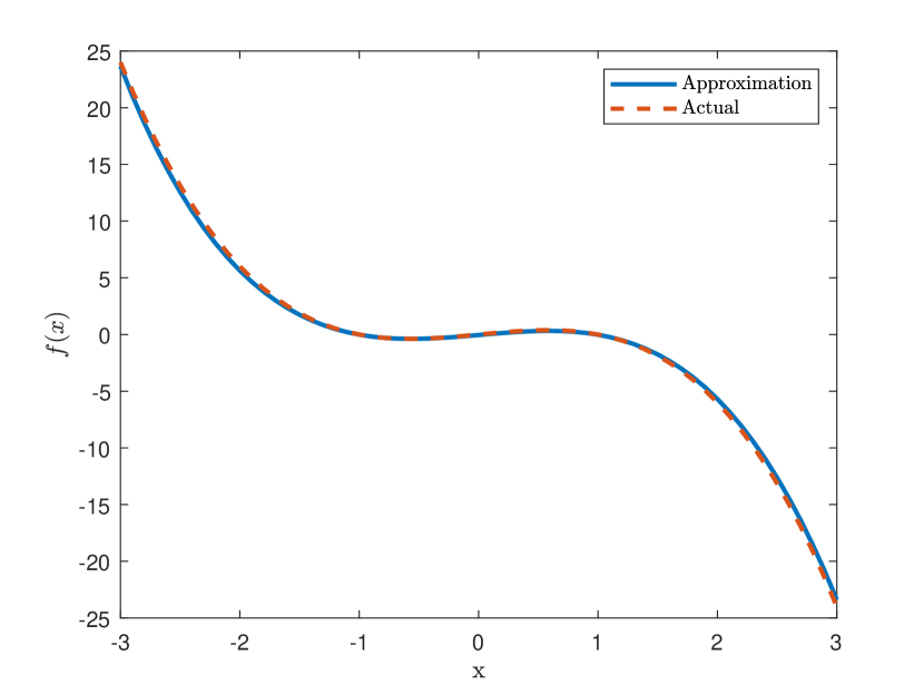
Figure 1: The evaluation of $f$ and $\hat{f}$ for the Duffing oscillator with measurement noise

Figure 2: The evaluation of $g$ and $\hat{g}$ for the Duffing oscillator with measurement noise

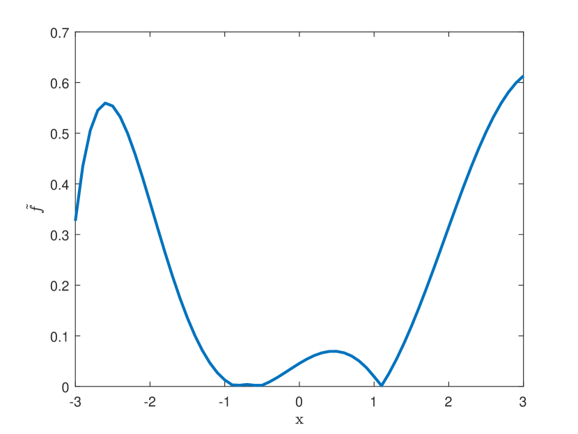
Figure 3: The evaluation of $\tilde{f}$ for the Duffing oscillator with measurement noise

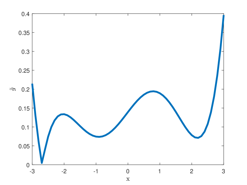
Figure 4: The evaluation of $\tilde{g}$ for the Duffing oscillator with measurement noise

Figure 1 shows the estimated and actual values of the drift function and Figure 2 shows the estimated and actual values of the control effectiveness function. Figure 3 shows the drift approximation error, $\tilde{f}$ as a function of $x$ and Figure 4 shows the control effectiveness approximation error, $\tilde{g}$, as a function of $x$.

A Monte-Carlo simulation with 1000 trials is conducted to evaluate robustness of the developed method to excitation signals and sensor noise, each trial uses 169 trajectories generated by a control signal that is composed of the sum of three sinusoidal signals with randomly generated frequencies and coefficients. Each trajectory is corrupted by Gaussian measurement noise with standard deviation 0.001. The initial velocities are obtained by numerically differentiating the measured noisy trajectories. For each trial, the mean of $\left|\tilde{f}\right|$ and $\left|\tilde{g}\right|$ evaluated at samples over the interval $[-3,3]$, are shown in Figures 5 and 6, respectively.

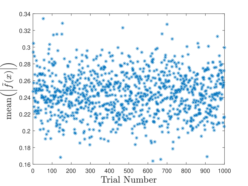
Figure 5: Monte-Carlo results of the mean of$\left|\tilde{f}\right|$ over 1000 trials

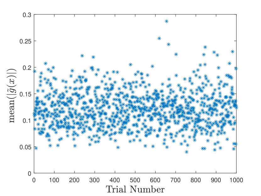
Figure 6: Monte-Carlo results of the mean of$\left|\tilde{g}\right|$ over 1000 trials

5.2 Control-affine model of a two-link robot manipulator

This experiment utilizes the first order four dimensional model of a two-link robot manipulator given by

$$M(q)\begin{pmatrix}\ddot{q_{1}}\\ \ddot{q_{2}}\end{pmatrix}=-C(q,\dot{q})+\tau$$ (6)

where $q_{1}$, and $q_{2}$ are the angular positions of the two links, respectively, $q:=\left(\begin{pmatrix}q_{1}\\ q_{2}\end{pmatrix}\right)$, $M(q)=\begin{pmatrix}p_{1}+2\cdot p_{3}\cos(q_{2})&p_{2}+p_{3}\cos(q_{2})\\ p_{2}+p_{3}\cos(q_{2})&p_{2}\end{pmatrix}$ is the inertia matrix, $C(q,\dot{q})=\left(V(q,\dot{q})+F_{d}\right)\begin{pmatrix}\dot{q_{1}}\\ \dot{q_{2}}\end{pmatrix}+F_{s}$, $F_{d}=\begin{pmatrix}f_{d_{1}}&0\\ 0&f_{d_{2}}\end{pmatrix}$ denotes viscous friction at the two joints, $F_{s}=\begin{pmatrix}f_{s_{1}}\tanh(\dot{q}_{1})\\ f_{s_{2}}\tanh(\dot{q}_{2})\end{pmatrix}$ denotes static friction at the two joints, $V(q,\dot{q})=\begin{pmatrix}-p_{3}\sin(q_{2})\dot{q_{2}}&-p_{3}\ \sin(q_{2})\cdot(\dot{q_{1}}+\dot{q_{2}})\\ p_{3}\sin(q_{2})\cdot\dot{q_{1}}&0\end{pmatrix}$ is the centrifugal-Coriolis matrix and $\tau=\begin{pmatrix}\tau_{1}\\ \tau_{2}\end{pmatrix}$ is the controller. The parameters are given by $p_{1}=3.473$, $p_{2}=0.196$, $p_{3}=0.242$, $f_{d_{1}}=5.3$, $f_{d_{2}}=1.1$, $f_{s_{1}}=8.45$, and $f_{s_{2}}=2.35$.

Then the system dynamics can be written as

$$\begin{pmatrix}\dot{q}\\ \ddot{q}\end{pmatrix}=\begin{pmatrix}\dot{q}\\ -M^{-1}(q)C(q,\dot{q})\end{pmatrix}+\begin{pmatrix}0&&0\\ 0&&0\\ \lx@intercol\hfil M^{-1}(q)\hfil\lx@intercol\end{pmatrix}\begin{pmatrix}\tau_{1}\\ \tau_{2}\end{pmatrix},$$ (7)

which is a four-dimensional first order control affine system of the form (1), with $f\left(\begin{pmatrix}q\\ \dot{q}\end{pmatrix}\right)=\begin{pmatrix}\dot{q}\\ -M^{-1}(q)C(q,\dot{q})\end{pmatrix}$, and $g\left(\begin{pmatrix}q\\ \dot{q}\end{pmatrix}\right)=\begin{pmatrix}0&&0\\ 0&&0\\ \lx@intercol\hfil M^{-1}(q)\hfil\lx@intercol\end{pmatrix}$.

Trajectories of the system are collected, starting from 1000 different initial conditions sampled using pseudorandom Halton sampling over a cube of side 6 centered at the origin of $\mathbb{R}^{4}$. Each trajectory is recorded using control signals $\tau_{1}$ and $\tau_{2}$, comprised of a sum of three sinusoidal signals with randomly generated frequencies and coefficients. For each run, the control signals and the trajectories of the system are recorded to generate the database that is used to approximate $f$ and $g$. Since this system has two controllers $\tau_{1}$ and $\tau_{2}$, the control effectiveness matrix $g$ is decomposed into $g_{1}$ and $g_{2}$, where $g_{1}$ is the first column of $g$ and $g_{2}$ is the second column of $g$.

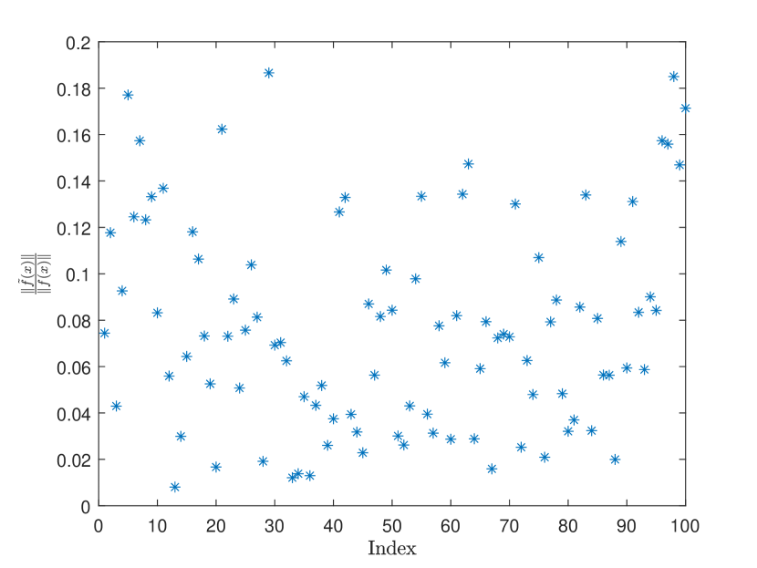
Figure 7: $\frac{\left\|\tilde{f}(x)\right\|}{\left\|f(x)\right\|}$ evaluated at 100 points, indexed by decreasing distance from the origin

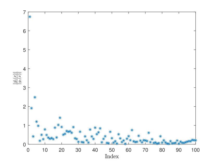
Figure 8: $\frac{\left\|\tilde{g_{1}}(x)\right\|}{\left\|g_{1}(x)\right\|}$ evaluated at 100 points, indexed by decreasing distance from the origin

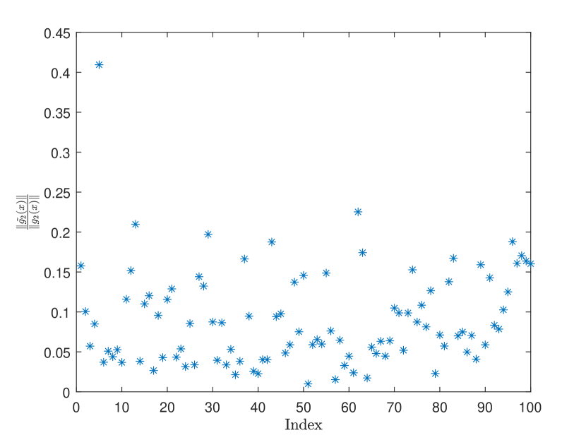
Figure 9: $\frac{\left\|\tilde{g_{2}}(x)\right\|}{\left\|g_{2}(x)\right\|}$ evaluated at 100 points, indexed by decreasing distance from the origin

The approximation error between the identified system and the actual system is computed through evaluation at 100 sample points sampled using pseudorandom Halton sampling over a cube of side 4 centered at the origin of $\mathbb{R}^{4}$. The functions $f$, $\hat{f}$, $g$, and $\hat{g}$ are evaluated at each vertex of the grid to yield the approximation errors $\tilde{f}$, $\tilde{g_{1}}$, and $\tilde{g_{2}}$.

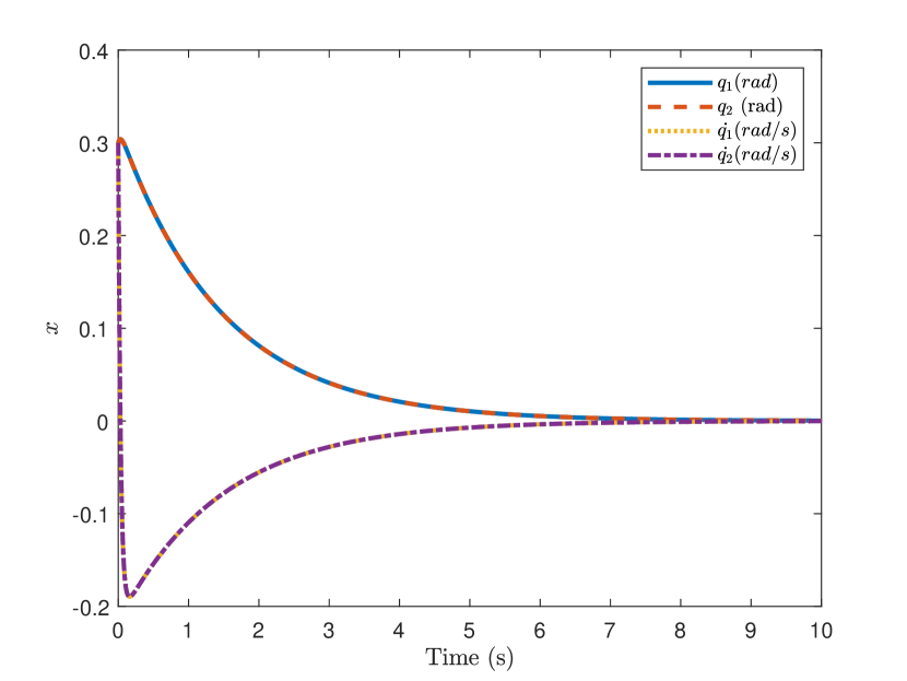
Figure 10: Regularization result using the true model for torque computation

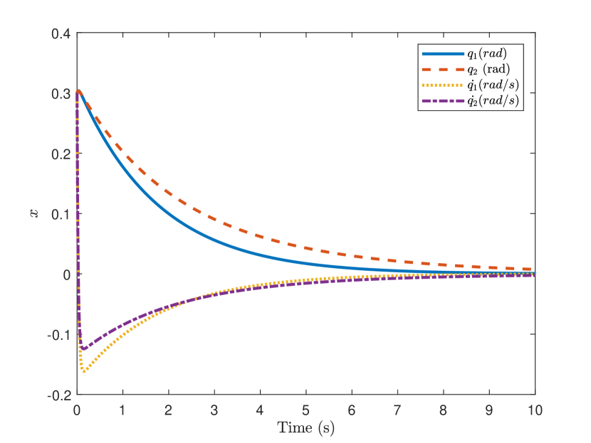
Figure 11: Regularization result using the Estimated model for torque computation

Figures 7, 9, and 9 shows the relative errors $\frac{\left\|\tilde{f}(x)\right\|}{\left\|f(x)\right\|}$, $\frac{\left\|\tilde{g_{1}}(x)\right\|}{\left\|g_{1}(x)\right\|}$, and $\frac{\left\|\tilde{g_{2}}(x)\right\|}{\left\|g_{2}(x)\right\|}$, respectively as a function of the node index.

To demonstrate the utility of the model developed via the novel system identification method, we simulate the actual two-link robot manipulator using a fourth order Runge-Kutta method with a computed torque controller designed to regulate the angular positions and velocities to zero. The computed torque controller is calculated using the estimated model, and is given by

$$\tau=\hat{M}(q)[-K_{v}\dot{q}-K_{p}q]+\hat{C}(q,\dot{q})$$ (8)

where $\hat{M}(q)$ and $\hat{C}(q,\dot{q})$ are recovered from the estimated data-driven drift and control-effectiveness functions $\hat{f}$ and $\hat{g}$, and $K_{p}=\begin{pmatrix}20&0\\ 0&20\end{pmatrix}$, $K_{v}=\begin{pmatrix}30&0\\ 0&30\end{pmatrix}$ are feedback gains.

Figure 11 shows the performance of the computed torque regulator used on the actual two-link robot manipulator.

6 Discussion

In the first numerical experiment, where the Duffing oscillator system is identified, the Control Occupation Kernel Regression method approximates $f$ and $g$. The approximation $\hat{f}$ is nearly identical to the true ${f}$ as seen in Figure 1 and the maximum error is $0.61$, which is a $2.6\%$ error as seen in Figure 3. The approximation $\hat{g}$ captures the underlining structure of $g$ where $g(x)=2+\sin(x)$, but $\hat{g}$ deviates slightly from the true value as seen in Figure 2 with a maximum error of $0.4$ which is a $23\%$ error as seen in Figure 4. The maximum errors are a function of kernel type, shape parameters, number and spatial coverage of the recorded data, and measurement noise, and can be reduced through segmentation of the recorded trajectories to generate more data points and increase the resolution of the approximations.

The Monte-Carlo trials summarized in Figures 5 and 6 demonstrate the robustness of the developed system identification method to excitation signals and measurement noise. Figures 1 and 2 show the full error plots of a representative sample trial.

In the second numerical experiment, where the model of a two-link robot manipulator is identified, Figures 7, 9, and 9 indicate that the estimation errors get worse as one approaches the boundary of the domain covered by the trajectories, and better as one approaches the origin. While the errors are hard to visualize as a function of distance from the training data in four dimensions, the trends observed in Figures 7, 9, and 9 could heuristically be attributed to limited coverage of the corners of the domain.

The identified system $\begin{pmatrix}\hat{f}(x)&\hat{g}(x)\end{pmatrix}$ is used to compute the necessary torque to regulate the actual two-link robot manipulator, which results in a performance, as seen in in Figure 11, similar to a computed torque controller implemented using exact model knowledge as seen in in Figure 11. The main downside of regulating the system using $\begin{pmatrix}\hat{f}(x)&\hat{g}(x)\end{pmatrix}$ is the long computation time necessary to evaluate $\begin{pmatrix}\hat{f}(x)&\hat{g}(x)\end{pmatrix}$ at any given $x$, which highlights the need for optimization of the evaluation function to improve computational performance.

7 Conclusion

A data-driven control occupation kernel regression method is developed in this manuscript for identification of nonlinear affine control systems, where identification of higher order systems is possible without numerical differentiation for higher order systems. As a result, as indicated by the numerical experiments, the developed method is robust to measurement noise. While it was demonstrated that the model developed using this method can be used to compute the feedforward component of a controller, depending on the number of trajectories used for modeling, evaluation of the model at a given state can be computationally expensive. Further research is required to develop a more efficient evaluation method to render it useful for real-time feedback.

A distinct advantage of the use of an occupation kernel basis to approximate the dynamics of the system is that under the assumptions of the framework developed in this paper, the solution of the minimization problem in (3) is guaranteed to be a linear combination of the occupation kernels by the representer theorem. This means that the occupation kernels are natural basis functions arising from a dynamics context, and in principle they should perform better than less structured bases. In particular, through the representer theorem, it is clear that the occupation kernel basis will, in general, result in models that yield a lower modeling error in the Hilbert space norm than any other generic basis, resulting in better generalization of the estimates away from the training data.

References

- [1] G. V. Chowdhary and E. N. Johnson, “Theory and flight-test validation of a concurrent-learning adaptive controller,” J. Guid. Control Dynam., vol. 34, no. 2, pp. 592–607, Mar. 2011.
- [2] S. L. Brunton, J. L. Proctor, and J. N. Kutz, “Discovering governing equations from data by sparse identification of nonlinear dynamical systems,” Proc. Nat. Acad. Sci. U.S.A., vol. 113, no. 15, pp. 3932–3937, 2016.
- [3] ——, “Sparse identification of nonlinear dynamics with control (SINDYc),” IFAC-PapersOnLine, vol. 49, no. 18, pp. 710–715, 2016. [Online]. Available: http://www.sciencedirect.com/science/article/pii/S2405896316318298
- [4] J. A. Rosenfeld, R. Kamalapurkar, B. Russo, and T. T. Johnson, “Occupation kernels and densely defined Liouville operators for system identification,” in Proc. IEEE Conf. Decis. Control, Dec. 2019, pp. 6455–6460. [Online]. Available: https://ieeexplore.ieee.org/document/9029337
- [5] J. B. Lasserre, D. Henrion, C. Prieur, and E. Trélat, “Nonlinear optimal control via occupation measures and LMI-relaxations,” SIAM J. Control Optim., vol. 47, no. 4, pp. 1643–1666, 2008.
- [6] A. Majumdar, R. Vasudevan, M. M. Tobenkin, and R. Tedrake, “Convex optimization of nonlinear feedback controllers via occupation measures,” Int. J. Robot. Res., vol. 33, no. 9, pp. 1209–1230, 2014.
- [7] M. Korda, D. Henrion, and C. N. Jones, “Controller design and value function approximation for nonlinear dynamical systems,” Automatica, vol. 67, pp. 54 – 66, 2016. [Online]. Available: http://www.sciencedirect.com/science/article/pii/S0005109816000236
- [8] B. Russo, R. Kamalapurkar, D. Chang, and J. A. Rosenfeld, “Motion tomography via occupation kernels,” arXiv:2101.02677, 2021. [Online]. Available: https://arxiv.org/abs/2101.02677
- [9] X. Li and J. A. Rosenfeld, “Fractional order system identification with occupation kernel regression,” IEEE Control Syst. Lett., to appear. [Online]. Available: https://ieeexplore.ieee.org/document/9305713
- [10] J. A. Rosenfeld, R. Kamalapurkar, L. F. Gruss, and T. T. Johnson, “On occupation kernels, Liouville operators, and dynamic mode decomposition,” in Proc. Am. Control Conf., May 2021, to appear, see arXiv:1910.03977.
- [11] J. A. Rosenfeld and R. Kamalapurkar, “Dynamic mode decomposition with control Liouville operators,” in Int. Symp. Math. Theory Netw. Syst., 2021, to appear, seearXiv:2101.02620.
- [12] G. S. Kimeldorf and G. Wahba, “A correspondence between Bayesian estimation on stochastic processes and smoothing by splines,” Ann. Math. Statist., vol. 41, pp. 495–502, 1970.