Multi-Objective SPIBB: Seldonian Offline Policy Improvement with Safety Constraints in Finite MDPs

Abstract

We study the problem of Safe Policy Improvement (SPI) under constraints in the offline Reinforcement Learning (RL) setting. We consider the scenario where: (i) we have a dataset collected under a known baseline policy, (ii) multiple reward signals are received from the environment inducing as many objectives to optimize. We present an SPI formulation for this RL setting that takes into account the preferences of the algorithm’s user for handling the trade-offs for different reward signals while ensuring that the new policy performs at least as well as the baseline policy along each individual objective. We build on traditional SPI algorithms and propose a novel method based on Safe Policy Iteration with Baseline Bootstrapping (SPIBB, laroche2017safe) that provides high probability guarantees on the performance of the agent in the true environment. We show the effectiveness of our method on a synthetic grid-world safety task as well as in a real-world critical care context to learn a policy for the administration of IV fluids and vasopressors to treat sepsis.

1 Introduction

Reinforcement Learning (RL) as a paradigm for sequential decision-making (sutton1988learning) has shown tremendous success in a variety of simulated domains (mnih2015human; silver2017mastering; OpenAI_dota). However, there are still quite a few challenges between the traditional RL research and real-world tasks. Most of these challenges stem from assumptions that are rarely satisfied in practice (dulac2019challenges), or the inability of the algorithm’s user to specify the desired behavior of the agent without being a domain expert (Thomas2019). We focus on the real-world application point of view and posit the following requirements:

• Multiple reward functions: Traditional RL methods assume a single scalar reward is present in the environment. However, most real-world tasks, have multiple (possibly conflicting) objectives or constraints that need to be taken into consideration together, such as the signals related to the safety (physical well-being of the agent or the environment), budget utilization (energy or maintenance costs), etc.

• Stakeholder control of the trade-off: The ML practitioners should have the ability to control the different trade-offs the agent is making and choose the one they consider best for the task at hand.

• Offline setting: In many real-world domains (e.g., healthcare, finance or autonomous vehicles), there is an abundance of data, collected under a sub-optimal policy, but training the agent directly via interactions with the environment is expensive and risky. We assume that we only have access to a dataset of past trajectories that can be used for training (lange2012batch).

• Preventing unintended behavior: We want the agent to be robust to both extrapolation errors from offline RL and misaligned objectives that are poor proxy of the user’s intentions and algorithm’s actual performance (ng1999policy; amodei2016concrete). We consider the case where the user can specify undesirable behavior in the context of the performance observed in the batch.

• Practical guarantees: We want guarantees about the undesirable behavior that might be caused by the agent in the real-world. We care about the results that can be obtained using the finite amount of samples we have in the batch, and aim to provide some measure of confidence in deploying the agents in the environment.

To achieve this set of properties, we adopt the Seldonian framework (Thomas2019), which is a general algorithm design framework that allows high-confidence guarantees for constraint satisfaction in a multi-objective setting. Based on the above specifications, we seek to answer the question: if we are given a batch of data collected under some (suboptimal) behavioral policy and some user preference, can we build a policy improvement algorithm that returns a policy with practical high-confidence guarantees on the performance of the policy w.r.t. the behavioral policy?

We acknowledge that there are other important challenges in RL, such as partial observability, safe exploration, non-stationary environments and function approximation in high-dimensional spaces, that also stand in the way of making RL a more applicable paradigm. These challenges are beyond the scope of this work, which should rather be thought of as taking a step towards this broader goal.

In Section 2, we present our contribution positioned with respect to other related work. In Section 3, we formalize the setting and then extend traditional SPI algorithms to this setting. We then show it is possible to extend the previous work on Safe Policy Iteration (SPI), particularly Safe Policy Iteration with Baseline Bootstrapping (SPIBB, laroche2017safe), for the design of agents that satisfy the above requirements. We show that the resulting algorithm is theoretically-grounded and provides practical high-probability guarantees. We extensively test our approach on a synthetic safety-gridworld task in LABEL:sec:synthetic-experiments and show that the proposed algorithm achieves better data efficiency than the existing approaches. Finally, we show its benefits on a critical-care task in LABEL:sec:sepsis-experiments. The accompanying codebase is available at https://github.com/hercky/mo-spibb-codebase.

2 Related work

Multi-Objective RL (MORL): Traditional multi-objective approaches (mannor2004geometric; roijers2013survey; liu2014multiobjective) focus on finding the Pareto-frontier of optimal reward functions that gives all the possible trade-offs between different objectives. The user can then select a policy from the solution set according to their arbitrary preferences. In practice, an alternate trial and error based approach of scalarization is used to transform the multiple reward functions into a scalar reward based on preferences across objectives (usually, by taking a linear combination). Most traditional MORL approaches have focused on the online, interactive settings where the agent has access to the environment. While some recent approaches are based on off-policy learning methods (lizotte2012linear; van2014multi; yang2019generalized; abdolmaleki2020distributional), they lack guarantees. In contrast, our work focuses exclusively on learning in the offline setting and gives high-probability guarantees on the performance in the environment.

Constrained-RL: RL under constraints frameworks, such as Constrained MDPs (CMDPs, altman1999constrained), present an alternative way to define preferences in the form of constraints over policy’s returns. Here, the user assigns a single reward function to be the primary objective (to maximize) and hard constraints are specified for the others. The major limitation of this setting is that it assumes the thresholds for the constraints are known a priori. le2019batch study offline policy learning under constraints and provide performance guarantees w.r.t. the optimal policy, but their work relies on the concentrability assumption (munos2003error).

Concentrability is a strong assumption that upper bounds the ratio between the future state-action distributions of any non-stationary policy and the baseline policy under which the dataset was generated by some constant. From a practical perspective, it is unclear how to get a tractable estimate of this constant, as the space of future state-action distributions of non-stationary policies is vast. Thus, this constant can be arbitrarily huge, potentially even infinite when the baseline policy fails to cover the support of the space of all non-stationary policies (such as in the low-data regime), leading to the performance bounds given by these methods to blow up (and even be unbounded). Additionally, the guarantees in le2019batch are only valid with respect to the performance of the optimal policy. In this work, we instead focus on the performance guarantees based on returns observed in the dataset, as it does not require making any of the above assumptions.

Reward design: Reward-design (sorg2010internal) and reward-modelling approaches (christiano2017deep; littman2017environment; leike2018scalable) focus on designing suitable reward functions that are consistent with the user’s intentions. These approaches rely heavily on the human or simulator feedback, and thus do not carry over easily to the offline setting.

Seldonian-RL (and Safe Policy Improvement): The Seldonian framework (Thomas2019) is a general algorithm design framework that allows the user to design ML algorithms that can avoid undesirable behavior with high-probability guarantees. In the context of RL, the Seldonian framework allows to design policy optimization problems with multiple constraints, where the solution policies satisfy the constraints with high-probability. In the offline-RL setting, SPI refers to the objective of guaranteeing a performance improvement over the baseline with high-probability guarantees (thomas2015highImprovement; petrik2016safe; laroche2017safe). Therefore, SPI algorithms are a specific setting that falls in the general category of Seldonian-RL algorithms.

We focus on two categories of SPI algorithms that provide practical error bounds on safety: SPIBB (laroche2017safe) that provides Bayesian bounds and HCPI (thomas2015highImprovement; thomas2015highEvaluation) that provides frequentist bounds. SPIBB methods constrain the change in the policy according to the local model uncertainty. SPIBB has been formulated in the context of a single reward function, and as such does not handle multiple rewards and by extension also lacks the ability for the user to specify preferences. Our primary focus is to provide a construction for extending the SPIBB methodology to the multi-objective setting that handles user preferences and provides high-probability guarantees.

Instead of relying on model uncertainty, HCPI methods utilize the high-confidence lower bounds on the Importance Sampling (IS) estimates of a target policy’s performance to ensure safety guarantees. HCPI has been applied to solve Seldonian optimization problems for constrained-RL setting using an enumerable policy class. Thomas2019 suggested using HCPI for the MORL setting, and we build on that idea. Particularly, we show how HCPI can be implemented with stochastic policies in the context of our setting with user preferences and baseline constraints.

3 Methodology

3.1 Setting

We consider the setting where the agent’s interactions with the environment can be modelled as a Markov Decision Process (MDP, bellman1957markovian). Let $\mathcal{X}$ and $\mathcal{A}$ respectively be the (finite) state and action spaces. Let $p^{\star}:\mathcal{X}\times\mathcal{A}\rightarrow\mathscr{P}(\mathcal{X})$ denote the true (unknown) transition probability function, where $\mathscr{P}(\mathcal{X})$ denotes the set of probability distributions on $\mathcal{X}$. Without loss of generality, we assume that the process deterministically begins in the state $x_{0}$. We define $[N]$ to be the set $\{0,1,\dots,N-1\}$ for any positive integer $N$. Let there be $d$ different reward signals and $\bm{r}^{\star}=\left\{r_{k}\right\}_{k\in[d]}:\mathcal{X}\times\mathcal{A}\rightarrow[-r_{\mathrel{\scalebox{0.5}{$\top$}}},r_{\mathrel{\scalebox{0.5}{$\top$}}}]^{d}$ be the true (unknown) stochastic multi-reward signal. Finally, $\bm{\gamma}=\left\{\gamma_{k}\right\}_{k\in[d]}\in[0,1)^{d}$ is the multi-discount-factor.

The MDP, $m^{\star}$, can now be defined with the tuple $(\mathcal{X},\mathcal{A},p^{\star},\bm{r}^{\star},\bm{\gamma},x_{0})$. A policy $\pi:\mathcal{X}\rightarrow\mathscr{P}(\mathcal{A})$ maps a state to a distribution over actions. We denote by $\Pi$ the set of stochastic policies. We consider the infinite horizon discounted return setting. For any $k\in[d]$, the $k$^th reward value function $v^{\pi}_{m,k}(x):\mathcal{X}\rightarrow\mathbb{R}$ denotes the expected discounted sum of rewards when when following policy $\pi$ in an MDP $m$ starting from state $x$. Analogously, we define the state-action value functions for performing action $a$ in state $x$ in MDP $m$ under $\pi$ for rewards as $q^{\pi}_{m,k}(x,a)$. Let $\operatorname*{Adv}^{\pi}_{m,k}(x,a)=q^{\pi}_{m,k}(x,a)-v^{\pi}_{m,k}(x)$ denote the corresponding advantage function. The expected return of policy $\pi$ w.r.t. the $k$^th reward in the true MDP $m^{\star}$ is denoted by $\mathcal{J}^{\pi}_{m^{\star},k}=v^{\pi}_{m^{\star},k}(x_{0})=\mathop{\mathbb{E}}_{\pi,m^{\star}}[\sum_{t=0}^{\infty}\gamma_{k}^{t}R_{k,t}\mid X_{0}=x_{0}]$, where action $A_{t}\sim\pi(\cdot\mid X_{t})$, immediate reward $R_{k,t}\sim r^{\star}_{k}(\cdot\mid X_{t},A_{t})$, and state $X_{t+1}\sim p^{\star}(\cdot\mid X_{t},A_{t})$.

We consider the offline setting, where instead of having access to the environment we have a pre-collected dataset of trajectories denoted by $\mathcal{D}=\{\tau_{i}\}_{i\in[|\mathcal{D}|]}$, where $|\mathcal{D}|$ denotes the number of trajectories in the dataset. A trajectory $\tau$ of length $T$ is an ordered set of transition tuples of the form $\tau=\{x_{i},a_{i},x^{\prime}_{i},\bm{r}_{i}\}_{i\in[T]}$, where $x^{\prime}_{i}$ denotes the state at the next time-step. We denote the Maximum Likelihood Estimation (MLE) of the MDP with $\hat{m}=(\mathcal{X},\mathcal{A},\hat{p},\hat{\bm{r}},\bm{\gamma},x_{0})$, where $\hat{p}$ and $\hat{\bm{r}}$ denote the transition and reward models estimated from the dataset’s statistics.

Assumption 3.1 (Baseline policy).

We assume that we have access to the policy that generated the dataset. We call such policy the baseline policy and denote it by $\pi_{b}$. 

3.2 Problem formulation

We consider safe policy improvement with respect to the baseline according to the $d$ dimensions of the multi-objective setting. Therefore, under a Bayesian approach, we search for target policies such that they perform better (up to a precision error $\zeta$) than the baseline along every objective function with high probability $1-\delta$, where $\zeta$ and $\delta$ are hyper-parameters controlled by the user, denoting the risk that the practitioner is willing to take. We denote by $\Pi_{\textsc{a}}$ the set of admissible policies that satisfy:

$$\mathbb{P}\left(\forall k\in[d],\mathcal{J}^{\pi}_{m^{\star},k}-\mathcal{J}^{\pi_{b}}_{m^{\star},k}>-\zeta\Big{|}\mathcal{D}\right)>1-\delta$$

In the multi-objective case, there does not exist a single optimal value, but a Pareto frontier of optimal values. One way to evaluate the MORL problems is via the multiple-policy approaches (vamplew2011empirical; roijers2013survey) that compute the policies that approximate the true optimal Pareto-frontier. However, note that optimality and safety are contradicting objectives. It is not clear how (and if) one can make claims about optimality in the offline setting without bringing in additional unrealistic assumptions (Section 2, MORL). Instead, we take an alternate approach inspired by another category of MORL methods called single-policy (roijers2013survey; van2014multi) where the trade-offs between different objectives are explicitly controlled by the user via providing a scalarization or preferences over objectives. We assume the user preference $\bm{\lambda}=\left\{\lambda_{k}\right\}_{k\in[d]}$ is given as an input to our algorithms, and is used for scalarization of the objectives, where $\lambda_{k}\in\mathbb{R}^{+}$. Our objective therefore becomes

$$\operatorname*{arg\,max}_{\pi\in\Pi_{\textsc{a}}} \quad\sum_{k\in[d]}\lambda_{k}\mathcal{J}^{\pi}_{m^{\star},k}$$

The above formulation gives freedom to the user in terms of what particular quantity they want to optimize via $\bm{\lambda}$, but still ensures that the solution policy performs as well as the baseline policy across all $d$ objectives. Note that our explicit goal is to maximize the objective specified by the user. However, the user might make mistakes in specifying this objective (Section 2, Reward design), and the above formulation offers guarantees that prevent deteriorating the performance of the policy across any of the $d$ objectives. This allows the user to to experiment with different reward design strategies in safety-critical settings without worrying about the risks of ill-defined scalarizations. A naïve approach would be applying the user scalarization to also define the safety constraints. However, this construction fails to prevent undesirable behavior for the individual objectives (shown in LABEL:app:naive-construction).

3.3 Multi-Objective SPIBB (MO-SPIBB)

Robust MDPs (Iyengar2005; Nilim2005) can be regarded as an approximation of the Bayesian formulation by partitioning the MDP space $\mathcal{M}$ into two subsets: the subset of plausible MDPs $\Xi$ and the subset of implausible MDPs. The plausible set is classically constructed from concentration bounds over the reward and transition function:

$$\Xi= \left\{m,\textnormal{ s.t. }\forall x,a,\begin{array}[]{ll}\lVert p(\cdot|x,a)-\hat{p}(\cdot|x,a)\rVert_{1}\leq e(x,a),\\ \lVert\bm{r}(x,a)-\hat{\bm{r}}(x,a)\rVert_{\infty}\leq e(x,a)r_{\mathrel{\scalebox{0.5}{$\top$}}}\end{array}\right\},$$

where $e$ is an upper bound on the state-action error function of the model that are classically obtained with concentration bounds, such that the true environment $m^{\star}\in\Xi$ with high probability $1-\delta$. In the single objective framework, laroche2017safe empirically show that optimising the worst-case performance policy in $\Xi$ provides policies that are too conservative. petrik2016safe prove that it is NP-hard to find the policy $\pi$ that maximises the worst-case policy improvement over $\Xi$.

Instead, the SPIBB methodology (laroche2017safe) consists in searching for a policy that maximizes the safe policy improvement in the MLE MDP, under some policy constraints: SPIBB and Soft-SPIBB (nadjahi2019safe) policy search constraints both revolve around the idea that we must only consider policies for which the policy improvement may be accurately estimated. Using $\pi_{b}$ as reference, SPIBB allows policy changes only in state-action pairs for which more than $n_{\wedge}$ samples have been collected. Soft-SPIBB extends this by applying soft constraints that allow slight changes in the policy for the uncertain state-action pairs, which are controlled by an error bound related to model uncertainty. As such, on low-confidence transitions, this class of methods provides a mechanism that prevents the agent from deviating too much from $\pi_{b}$. In this work, we build on Soft-SPIBB because it has yielded better empirical results. Formally, its constraint on the policy class is defined by:

$$\Pi_{\textsc{s}}=\left\{\pi,\text{ s.t. }\forall x,\sum_{a}e(x,a)\ |\pi(a|x)-\pi_{b}(a|x)|\leq\epsilon\right\},$$

where $\epsilon$ is a hyper-parameter that controls the deviation from the baseline policy.

We define $q^{\pi}_{m,\bm{\lambda}}(x,a)=\sum_{k\in[d]}\lambda_{k}q^{\pi}_{m,k}(x,a)$ to be the state-action value function associated with the linearized $\bm{\lambda}$ parameters. The same notation extension is used for $v^{\pi}_{m,\bm{\lambda}}(x,a)$ and $\mathcal{J}^{\pi}_{m,\bm{\lambda}}$. The application of Soft-SPIBB to multi-objective safe policy improvement is therefore direct: Figure 7: Results on 100 random CMDPs for different $\bm{\lambda}$ and $\rho$ combinations with $\delta=0.1$. The different agents are represented by different markers and colored lines. Each point on the plot denotes the mean (with standard error bars) for 12 different $\bm{\lambda},\rho$ combinations for the 100 randomly generated CMDPs (1200 datapoints). The x-axis denotes the amount of data the agents were trained on. The y-axis for left subplot in each sub-figure represents the improvement over baseline and the right subplot denotes the failure rate. The dotted black line in the right subplots represents the high-confidence parameter $\delta=0.1$. LABEL:fig:lag-only-single-sopt denotes the case when MO-SPIBB (LABEL:eq:s-opt) is run with $\epsilon=0.1$, MO-HCPI (LABEL:eq:h-opt) with $\text{IS}=$ Doubly Robust (DR) estimator with student’s t-test concentration inequality, and Lagrangian (le2019batch) with $\eta=0.01$ . Figure 7(b) shows how MO-SPIBB and Lagrangian perform across different hyper-parameters.

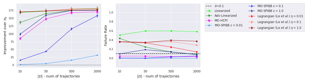
(b) MO-SPIBB (LABEL:eq:s-opt) and Lagrangian (le2019batch) comparisons across different hyper-parameters.

We test the method by le2019batch (henceforth referred to as Lagrangian) in the synthetic navigation CMDP task described in LABEL:sec:synthetic-experiments. In LABEL:fig:lag-only-single-sopt, we present the results for the best performing Lagrangian baseline on 100 random CMDPs for different $\bm{\lambda}$ and $\rho$ combinations with $\delta=0.1$. Similar to LABEL:fig:delta-params-mean, we provide a more detailed plot of how the Lagrangian baseline performs with different hyper-parameters in the above setting in Figure 7(b).

Results: As expected, we observe that the Lagrangian baseline has a high failure rate, particularly in the low-data setting. This makes sense as the guarantees provided by le2019batch are of the form $\mathcal{J}^{\pi}_{k,m^{\star}}-\mathcal{J}^{\pi_{b}}_{k,m^{\star}}\geq-\frac{C}{(1-\gamma)^{3/2}}$ (Theorem 4.4 of le2019batch), where $C$ is a term that depends on a constant that comes from the Concentrability assumption (Assumption 1 of le2019batch). This assumption upper bounds the ratio between the future state-action distributions of any non-stationary policy and the baseline policy under which the dataset was generated by some constant. In other words, it makes assumptions on the quality of the data gathered under the baseline policy. Unfortunately, this assumption cannot be verified in practice, and it is unclear how to get a tractable estimate of this constant. As such, this constant can be arbitrarily large (even infinite) when the baseline policy fails to cover the support of all non-stationary policies, for instance, when the baseline policy is not exploratory enough or when the size of the dataset is small. Hence, we observe a high failure rate of le2019batch in the experiments, especially in the low data setting. Compared to le2019batch, our performance guarantees do not make any assumptions on the quality of the dataset or the baseline. Therefore, our approach can ensure a low failure rate even in the low-data regime.

Implementation details and Hyper-parameters: We build on top of the publicly available code of le2019batch released by the authors and extend it to our setting. We are confident that our implementation is correct as we made sure it passes various sanity tests such as convergence of the primal-dual gap and feasibility on access to true MDP parameters.

The algorithm in le2019batch (Algorithm 2, Constrained Batch Policy Learning) requires the following hyper-parameters:

• Online Learning Subroutine: We use the same online learning algorithm as used by the authors in their experiments, i.e. Exponentiated Gradient (kivinen1997exponentiated).

• Duality gap $\omega$ : This denotes the primal-dual gap or the early termination condition. We tried the values in $\{0.01,0.001\}$ and fix the value to $0.01$.

• Number of iterations: This parameter denotes the number of iterations for which the Lagrange coefficients should be updated. We experimented in the range $\{100,250,500\}$ and set this to $250$.

• Norm bound $B$: The bound on the norm of Lagrange coefficients vector. We tried the values in $\{1,10,50,100\}$ and fixed it $10$.

• Learning rate $\eta$: This parameter denotes the learning rate for the update of the Lagrange coefficients via the online learning subroutine. We found that this is the most sensitive variable and we tried with values in $\{0.005,0.01,0.05,0.1,0.5,1.0,5.0\}$. For the final experiments, we benchmark with three different values $(0.01,0.1,1.0)$ as mentioned in the Figure 7(b).

We would like to point out that the hyper-parameter tuning for the Lagrangian baseline can be particularly challenging as in the low-data setting none of the combinations of the above hyper-parameters can ensure a low failure rate even though the duality gap has converged.

The above experiments show the advantage of our approach over le2019batch, particularly in the low-data safety-critical tasks, where our methods can improve over the baseline policy while ensuring a low failure rate.

D.5 Scaling experiments with number of objectives $d$

We experimented with the different number of objectives $d$ to validate if the trends we observed for LABEL:eq:s-opt and LABEL:eq:h-opt in LABEL:sec:synthetic-experiments also extend to $d>2$. In the CMDP formulation, as there can only be one primary reward, we extend the CMDP to include more than 1 type of pits. The extended CMDP now has $d-1$ different kinds of pits and corresponding reward functions, where the agent gets a pit reward of $-1$ if the agent steps into a cell containing that particular kind of pit. We relax the CMDP threshold to $c_{i}=-10.0$ as the CMDP problem gets harder with more number of pits, and a lower threshold makes the problem of finding $\pi^{*}$ of a random CMDP easier. Therefore, the task objective for the agent in the extended CMDP is to reach the goal in the least amount of steps, such that it can only step into at most 10 pits of every different type.

We use the same experiment methodology from LABEL:sec:synthetic-experiments. As the focus is to see how the trends scale with $d$, we fix the $\bm{\lambda}$, with $\lambda_{0}=1.0$ and the rest of $\lambda_{\geq 1}=0.0$. We compare LABEL:eq:s-opt and LABEL:eq:h-opt over different $|\mathcal{D}|\in\{10,50,500,2000\}$, $\rho\in\{0.1,0.4,0.7,0.9\}$, the fixed set of parameters: IS=DR, $\text{CI}=$student’s t-test, $\epsilon\in\{0.001,0.01,0.1,1.0\}$, and $\delta=0.1$.

The results over 10 random CMDPs with fixed parameters can be found in Figure 8. We notice that the trends from LABEL:sec:synthetic-experiments case still carry till $d\leq 1+16$, where for some value of $\epsilon$, LABEL:eq:s-opt can lead to better improvement in $\pi_{b}$ while still having failure rate $<\delta$. However, $d>1+16$ we see there are no obvious trends and both LABEL:eq:s-opt and LABEL:eq:h-opt tend to become very conservative and returning the baseline becomes the best solution choice.

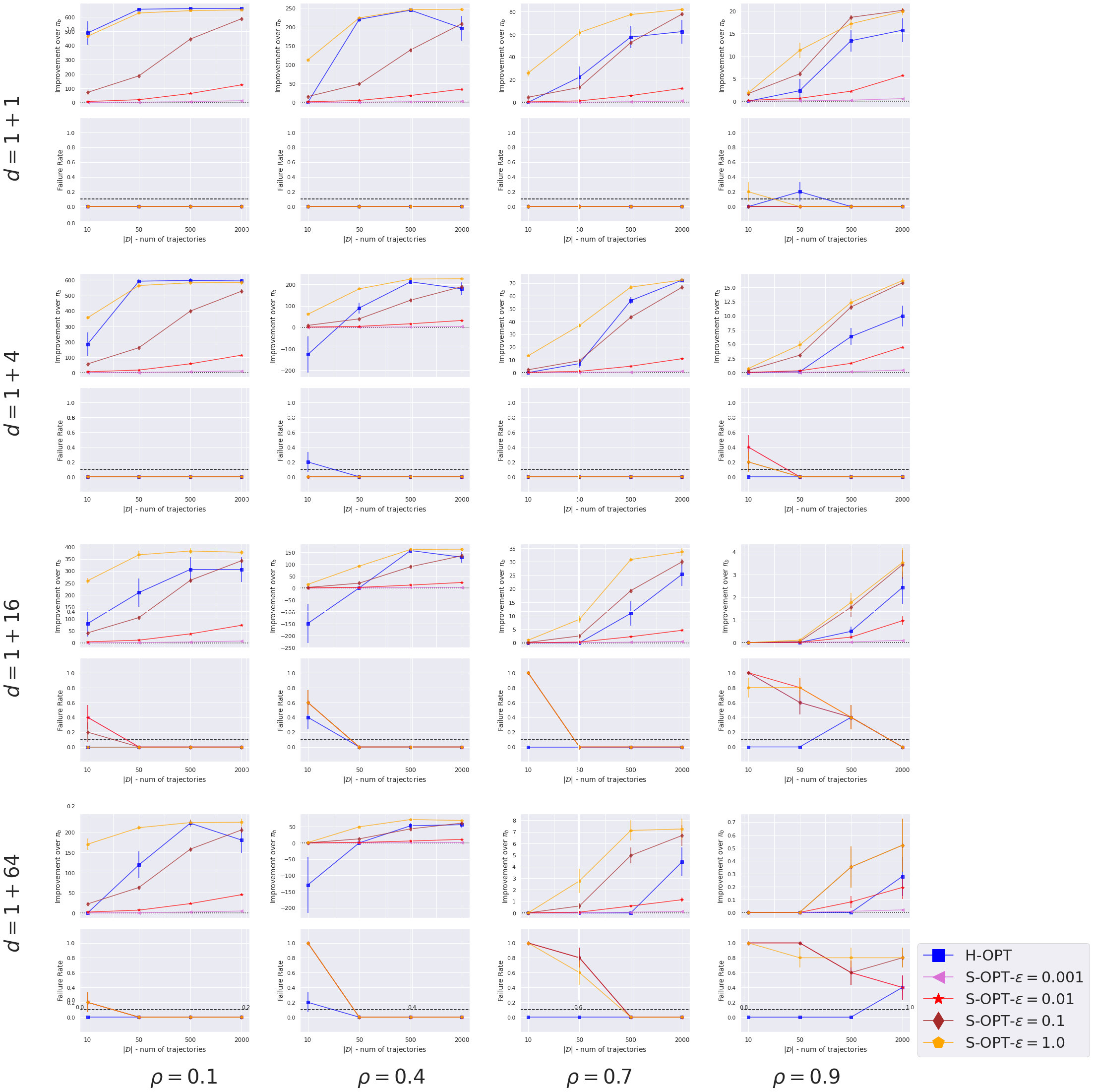
Figure 8: Scaling with $d$ with results on a 10 random CMDPs and $\delta=0.1$. The different agents are represented by different markers and color. Each point on the graph denotes the mean for 100 runs, the standard errors is denoted by the error bars. The x-axis denotes the amount of data the agents were trained on. They y-axis for the top plot in a grid represents the improvement over baseline and the y-axis for bottom plot denotes the failure rate.

D.6 Additional details

For the experiments in LABEL:sec:synthetic-experiments, on an Intel(R) Xeon(R) Gold 6230 CPU (2.10GHz), the baselines take around 3 seconds to run, and both LABEL:eq:s-opt and LABEL:eq:h-opt take about 5 seconds.

Appendix E Additional details for sepsis experiments

E.1 Sepsis data and cohort details

We followed the pre-processing methodology from tang2020clinician; komorowski2018artificial and we refer the reader to the original work for more details.

The dosage of prescribed IV fluids and vasopressors is converted into discrete variables to be used as actions for the constructed MDP. Each type of action (IV or vasopressor) is divided into 4 bins (each representing one quantile), and an additional action for "No drug" (0 dose) is also introduced. As such, the $|\mathcal{A}|=5\times 5$. The cohort statistics can be found in Table 2. The patient data consists of 48 dimensional time-series with features representing attributes such as demographics, vitals and lab work results (Table 3). The patient data is discretized into 4-hour windows, each of which is pre-processed to be treated as a single time-step. The state-space and is discretized using a k-means based clustering algorithm to map the states to $750$ clusters. Two additional absorbing states are added for death and survival ($|\mathcal{X}|=752$).

Table 2: Cohort statistics after following the data pre-processing methodology from tang2020clinician; komorowski2018artificial.

Survivors	N	% Female	Mean Age	Hours in ICU
Survivors	18066	44.5%	64.1	56.6
Non-survivors	2888	42.9%	68.8	60.9

Table 3: Summary of the patient state features from (tang2020clinician, Table 3).

Demographics/Static	Age, Gender, SOFA, Shock Index, Elixhauser, SIRS, Re-admission, GCS - Glasgow Coma Scale
Lab values	Albumin, Arterial pH, Calcium, Glucose, Hemoglobin, Magnesium, PTT - Partial Thromboplastin Time, Potassium, SGPT - Serum Glutamic-Pyruvic Transaminase, Arterial Blood Gas, Blood Urea Nitrogen, Chloride, Bicarbonate, International Normalized Ratio, Sodium, Arterial Lactate, CO2, Creatinine, Ionised Calcium, Prothrombin Time, Platelets Count, SGOT - Serum Glutamic-Oxaloacetic Transaminase, Total bilirubin, White Blood Cell Count
Vital signs	Diastolic Blood Pressure, Systolic Blood Pressure, Mean Blood Pressure, PaCO2, PaO2, FiO2, PaO/FiO2 ratio, Respiratory Rate, Temperature (Celsius), Weight (kg), Heart Rate, SpO2
Intake and output events	Fluid Output - 4 hourly period, Total Fluid Output, Mechanical Ventilation

E.2 Performance on changing hyper-parameters

For the experiments in LABEL:sec:sepsis-experiments, we treat $\delta$ as a hyper-parameter. For LABEL:eq:s-opt instead of searching over both $\delta$ and $\epsilon$, we follow the strategy proposed in Soft-SPIBB: fix the $\delta=1.0$ and only search over $\epsilon$. For LABEL:eq:h-opt, we found that only DR and WDR gave reliable off-policy estimates so report the results with both of them with different $\delta$. As in previous sections, we used student’s t-test as the choice of concentration inequality for LABEL:eq:h-opt.

E.2.1 LABEL:eq:s-opt parameters

Here, we fix $\delta=1.0$ and try with different values of the hyper-parameter $\epsilon$ and directly report the results directly on the test set. The results are presented in Table 4.

E.2.2 LABEL:eq:h-opt parameters

We run with different values of the hyper-parameter $\delta$ and directly report the results directly on the test set for different IS estimators. The results for DR estimator are presented in Table 4 and for WDR estimator are presented in Table 4.

E.3 Additional qualitative Analysis

We calculate how many rare-actions are recommended by different solution policies and compare them with the most common actions taken by the clinicians. For each state, for the action recommended by a solution policy, we calculate the frequency with which that state-action was observed in the training data and calculate the percentage of time that state-action pair was observed among all the possible actions taken from that state. Across all the states, the actions suggested by the traditional single-objective RL baseline are observed only 3% of the time on average (5.3 observations per state). Whereas, the actions most commonly chosen by the clinicians are observed 51.4% of the time on average (138.2 observations per state). We study this behavior for two of the policies returned by MO-SPIBB that deviate the most from the baseline: for the policy returned by LABEL:eq:s-opt ($\bm{\lambda}=[1,1]$) the recommended actions are observed 24.8% of time on average (61.0 observations per state) and for LABEL:eq:s-opt ($\bm{\lambda}=[0,1]$) the recommended actions are observed 23.4% of times (56.14 observations per state).

E.4 Additional details

For the experiments in LABEL:sec:sepsis-experiments, on an Intel(R) Xeon(R) Gold 6230 CPU (2.10GHz), running the Linearized baseline takes around 30 seconds, Adv-Linearized takes around 60 seconds, LABEL:eq:s-opt take about 90-120 seconds and LABEL:eq:h-opt takes about 90 seconds.

Table 4: Performance of various LABEL:eq:s-opt policy candidates (with different $\epsilon$) using DR and WDR estimation with standard errors on 10 random splits of the TEST dataset. The red cells denote the corresponding safety constraint violation, i.e, either $\mathcal{J}_{0}^{\pi}<\mathcal{J}_{0}^{\pi_{b}}$ or $-\mathcal{J}_{1}^{\pi}>-\mathcal{J}_{1}^{\pi_{b}}$.

User preferences $(\bm{\lambda})$ Policy Survival return ($\mathcal{J}_{0}$) Rare-treatment return ($-\mathcal{J}_{1}$) DR WDR DR WDR Clinician’s ($\pi_{b}$) 64.78 $\pm$ 0.90 64.78 $\pm$ 0.90 13.58 $\pm$ 0.19 13.58 $\pm$ 0.19 $[\lambda_{0}=1.0,\lambda_{1}=0.0]$ Linearized 97.68 $\pm$ 0.22 97.58 $\pm$ 0.20 27.64 $\pm$ 1.11 27.84 $\pm$ 1.09 LABEL:eq:s-opt, $\epsilon=0.0$ 64.78 $\pm$ 0.90 64.78 $\pm$ 0.90 13.58 $\pm$ 0.19 13.58 $\pm$ 0.19 LABEL:eq:s-opt, $\epsilon=0.001$ 64.91 $\pm$ 0.90 64.91 $\pm$ 0.90 13.56 $\pm$ 0.19 13.56 $\pm$ 0.19 LABEL:eq:s-opt, $\epsilon=0.01$ 66.11 $\pm$ 0.87 66.05 $\pm$ 0.86 13.42 $\pm$ 0.20 13.46 $\pm$ 0.20 LABEL:eq:s-opt, $\epsilon=0.1$ 73.70 $\pm$ 0.84 71.96 $\pm$ 0.69 12.30 $\pm$ 0.39 13.80 $\pm$ 0.33 LABEL:eq:s-opt, $\epsilon=0.5$ 78.19 $\pm$ 0.54 81.01 $\pm$ 0.36 16.21 $\pm$ 0.49 13.10 $\pm$ 0.31 LABEL:eq:s-opt, $\epsilon=1.0$ 84.03 $\pm$ 0.48 87.11 $\pm$ 0.33 15.54 $\pm$ 0.59 12.17 $\pm$ 0.59 LABEL:eq:s-opt, $\epsilon=2.5$ 90.05 $\pm$ 0.25 91.37 $\pm$ 0.20 15.35 $\pm$ 0.72 13.53 $\pm$ 0.56 LABEL:eq:s-opt, $\epsilon=5.0$ 91.58 $\pm$ 0.49 92.66 $\pm$ 0.28 15.39 $\pm$ 0.59 13.71 $\pm$ 0.38 LABEL:eq:s-opt, $\epsilon=10.0$ 91.64 $\pm$ 0.47 92.68 $\pm$ 0.23 15.19 $\pm$ 0.59 13.56 $\pm$ 0.42 LABEL:eq:s-opt, $\epsilon=\infty$ 91.62 $\pm$ 0.46 92.68 $\pm$ 0.23 15.18 $\pm$ 0.59 13.56 $\pm$ 0.42 $[\lambda_{0}=1.0,\lambda_{1}=1.0]$ Linearized 87.17 $\pm$ 0.48 89.11 $\pm$ 0.37 2.41 $\pm$ 0.47 1.52 $\pm$ 0.41 LABEL:eq:s-opt, $\epsilon=0.0$ 64.78 $\pm$ 0.90 64.78 $\pm$ 0.90 13.58 $\pm$ 0.19 13.58 $\pm$ 0.19 LABEL:eq:s-opt, $\epsilon=0.001$ 64.90 $\pm$ 0.90 64.90 $\pm$ 0.90 13.53 $\pm$ 0.19 13.54 $\pm$ 0.19 LABEL:eq:s-opt, $\epsilon=0.01$ 66.02 $\pm$ 0.88 65.94 $\pm$ 0.87 13.15 $\pm$ 0.20 13.20 $\pm$ 0.20 LABEL:eq:s-opt, $\epsilon=0.1$ 74.34 $\pm$ 0.78 72.04 $\pm$ 0.87 9.32 $\pm$ 0.29 10.48 $\pm$ 0.45 LABEL:eq:s-opt, $\epsilon=0.5$ 76.47 $\pm$ 0.50 78.42 $\pm$ 0.41 7.61 $\pm$ 0.44 5.02 $\pm$ 0.17 LABEL:eq:s-opt, $\epsilon=1.0$ 81.39 $\pm$ 0.46 84.54 $\pm$ 0.36 4.64 $\pm$ 0.40 2.38 $\pm$ 0.22 LABEL:eq:s-opt, $\epsilon=2.5$ 86.26 $\pm$ 0.33 88.09 $\pm$ 0.24 1.98 $\pm$ 0.28 1.14 $\pm$ 0.27 LABEL:eq:s-opt, $\epsilon=5.0$ 86.76 $\pm$ 0.47 88.55 $\pm$ 0.22 2.52 $\pm$ 0.48 1.55 $\pm$ 0.41 LABEL:eq:s-opt, $\epsilon=10.0$ 86.77 $\pm$ 0.49 88.58 $\pm$ 0.25 2.53 $\pm$ 0.50 1.57 $\pm$ 0.43 LABEL:eq:s-opt, $\epsilon=\infty$ 86.77 $\pm$ 0.49 88.58 $\pm$ 0.25 2.53 $\pm$ 0.50 1.57 $\pm$ 0.43 $[\lambda_{0}=0.0,\lambda_{1}=0.0]$ Linearized -89.39 $\pm$ 0.43 -90.90 $\pm$ 0.29 22.99 $\pm$ 0.40 22.81 $\pm$ 0.30 LABEL:eq:s-opt, $\epsilon=0.0$ 64.78 $\pm$ 0.90 64.78 $\pm$ 0.90 13.58 $\pm$ 0.19 13.58 $\pm$ 0.19 LABEL:eq:s-opt, $\epsilon=0.001$ 64.80 $\pm$ 0.90 64.80 $\pm$ 0.90 13.57 $\pm$ 0.19 13.57 $\pm$ 0.19 LABEL:eq:s-opt, $\epsilon=0.01$ 64.92 $\pm$ 0.90 64.92 $\pm$ 0.90 13.50 $\pm$ 0.19 13.51 $\pm$ 0.19 LABEL:eq:s-opt, $\epsilon=0.1$ 65.78 $\pm$ 0.89 65.70 $\pm$ 0.88 13.20 $\pm$ 0.20 13.25 $\pm$ 0.20 LABEL:eq:s-opt, $\epsilon=0.5$ 67.73 $\pm$ 0.82 67.22 $\pm$ 0.88 13.24 $\pm$ 0.24 13.55 $\pm$ 0.33 LABEL:eq:s-opt, $\epsilon=1.0$ 69.12 $\pm$ 0.75 67.90 $\pm$ 0.84 13.57 $\pm$ 0.27 14.39 $\pm$ 0.44 LABEL:eq:s-opt, $\epsilon=2.5$ 71.00 $\pm$ 0.63 68.28 $\pm$ 0.46 14.27 $\pm$ 0.30 15.73 $\pm$ 0.40 LABEL:eq:s-opt, $\epsilon=5.0$ 71.95 $\pm$ 0.54 69.27 $\pm$ 0.63 15.29 $\pm$ 0.39 16.12 $\pm$ 0.70 LABEL:eq:s-opt, $\epsilon=10.0$ 72.73 $\pm$ 0.64 71.17 $\pm$ 0.65 16.59 $\pm$ 0.37 16.21 $\pm$ 0.41 LABEL:eq:s-opt, $\epsilon=\infty$ 60.27 $\pm$ 0.49 61.44 $\pm$ 0.85 18.40 $\pm$ 0.27 15.36 $\pm$ 0.58 $[\lambda_{0}=0.0,\lambda_{1}=1.0]$ Linearized 58.27 $\pm$ 2.18 60.52 $\pm$ 2.07 0.04 $\pm$ 0.03 0.02 $\pm$ 0.01 LABEL:eq:s-opt, $\epsilon=0.0$ 64.78 $\pm$ 0.90 64.78 $\pm$ 0.90 13.58 $\pm$ 0.19 13.58 $\pm$ 0.19 LABEL:eq:s-opt, $\epsilon=0.001$ 64.83 $\pm$ 0.90 64.83 $\pm$ 0.90 13.52 $\pm$ 0.19 13.52 $\pm$ 0.19 LABEL:eq:s-opt, $\epsilon=0.01$ 65.36 $\pm$ 0.88 65.27 $\pm$ 0.88 12.96 $\pm$ 0.19 13.01 $\pm$ 0.19 LABEL:eq:s-opt, $\epsilon=0.1$ 71.35 $\pm$ 0.96 69.29 $\pm$ 0.92 7.75 $\pm$ 0.19 8.30 $\pm$ 0.18 LABEL:eq:s-opt, $\epsilon=0.5$ 71.01 $\pm$ 0.72 71.30 $\pm$ 0.68 2.54 $\pm$ 0.37 1.50 $\pm$ 0.11 LABEL:eq:s-opt, $\epsilon=1.0$ 74.19 $\pm$ 0.57 76.11 $\pm$ 0.57 0.90 $\pm$ 0.14 0.34 $\pm$ 0.09 LABEL:eq:s-opt, $\epsilon=2.5$ 76.42 $\pm$ 0.61 77.20 $\pm$ 0.72 0.10 $\pm$ 0.06 0.06 $\pm$ 0.04 LABEL:eq:s-opt, $\epsilon=5.0$ 76.08 $\pm$ 0.65 76.87 $\pm$ 0.74 0.07 $\pm$ 0.05 0.05 $\pm$ 0.03 LABEL:eq:s-opt, $\epsilon=10.0$ 76.07 $\pm$ 0.65 76.87 $\pm$ 0.73 0.07 $\pm$ 0.05 0.04 $\pm$ 0.03 LABEL:eq:s-opt, $\epsilon=\infty$ 76.05 $\pm$ 0.65 76.85 $\pm$ 0.72 0.07 $\pm$ 0.05 0.04 $\pm$ 0.03

Table 4: Performance of various LABEL:eq:h-opt policy candidates (with different $\delta$) using $\text{IS}=$ DR estimator with standard errors on 10 random splits of the TEST dataset. The red cells denote the corresponding safety constraint violation, i.e, either $\mathcal{J}_{0}^{\pi}<\mathcal{J}_{0}^{\pi_{b}}$ or $-\mathcal{J}_{1}^{\pi}>-\mathcal{J}_{1}^{\pi_{b}}$.

User preferences $(\bm{\lambda})$ Policy Survival return ($\mathcal{J}_{0}$) Rare-treatment return ($-\mathcal{J}_{1}$) DR WDR DR WDR Clinician’s ($\pi_{b}$) 64.78 $\pm$ 0.90 64.78 $\pm$ 0.90 13.58 $\pm$ 0.19 13.58 $\pm$ 0.19 $[\lambda_{0}=1.0,\lambda_{1}=0.0]$ Linearized 97.68 $\pm$ 0.22 97.58 $\pm$ 0.20 27.64 $\pm$ 1.11 27.84 $\pm$ 1.09 LABEL:eq:h-opt, $\delta=0.1$ 65.95 $\pm$ 0.00 65.95 $\pm$ 0.00 13.37 $\pm$ 0.00 13.37 $\pm$ 0.00 LABEL:eq:h-opt, $\delta=0.3$ 65.95 $\pm$ 0.00 65.95 $\pm$ 0.00 13.37 $\pm$ 0.00 13.37 $\pm$ 0.00 LABEL:eq:h-opt, $\delta=0.5$ 65.95 $\pm$ 0.00 65.95 $\pm$ 0.00 13.37 $\pm$ 0.00 13.37 $\pm$ 0.00 LABEL:eq:h-opt, $\delta=0.7$ 65.95 $\pm$ 0.00 65.95 $\pm$ 0.00 13.37 $\pm$ 0.00 13.37 $\pm$ 0.00 LABEL:eq:h-opt, $\delta=0.9$ 65.95 $\pm$ 0.00 65.95 $\pm$ 0.00 13.37 $\pm$ 0.00 13.37 $\pm$ 0.00 $[\lambda_{0}=1.0,\lambda_{1}=1.0]$ Linearized 87.17 $\pm$ 0.48 89.11 $\pm$ 0.37 2.41 $\pm$ 0.47 1.52 $\pm$ 0.41 LABEL:eq:h-opt, $\delta=0.1$ 86.37 $\pm$ 0.00 88.03 $\pm$ 0.00 2.58 $\pm$ 0.00 1.43 $\pm$ 0.00 LABEL:eq:h-opt, $\delta=0.3$ 86.37 $\pm$ 0.00 88.03 $\pm$ 0.00 2.58 $\pm$ 0.00 1.43 $\pm$ 0.00 LABEL:eq:h-opt, $\delta=0.5$ 86.37 $\pm$ 0.00 88.03 $\pm$ 0.00 2.58 $\pm$ 0.00 1.43 $\pm$ 0.00 LABEL:eq:h-opt, $\delta=0.7$ 86.37 $\pm$ 0.00 88.03 $\pm$ 0.00 2.58 $\pm$ 0.00 1.43 $\pm$ 0.00 LABEL:eq:h-opt, $\delta=0.9$ 86.37 $\pm$ 0.00 88.03 $\pm$ 0.00 2.58 $\pm$ 0.00 1.43 $\pm$ 0.00 $[\lambda_{0}=0.0,\lambda_{1}=0.0]$ Linearized -89.39 $\pm$ 0.43 -90.90 $\pm$ 0.29 22.99 $\pm$ 0.40 22.81 $\pm$ 0.30 LABEL:eq:h-opt, $\delta=0.1$ 65.95 $\pm$ 0.00 65.95 $\pm$ 0.00 13.37 $\pm$ 0.00 13.37 $\pm$ 0.00 LABEL:eq:h-opt, $\delta=0.3$ 65.95 $\pm$ 0.00 65.95 $\pm$ 0.00 13.37 $\pm$ 0.00 13.37 $\pm$ 0.00 LABEL:eq:h-opt, $\delta=0.5$ 65.95 $\pm$ 0.00 65.95 $\pm$ 0.00 13.37 $\pm$ 0.00 13.37 $\pm$ 0.00 LABEL:eq:h-opt, $\delta=0.7$ 68.28 $\pm$ 0.00 63.25 $\pm$ 0.00 14.16 $\pm$ 0.00 16.41 $\pm$ 0.00 LABEL:eq:h-opt, $\delta=0.9$ 68.28 $\pm$ 0.00 63.25 $\pm$ 0.00 14.16 $\pm$ 0.00 16.41 $\pm$ 0.00 $[\lambda_{0}=0.0,\lambda_{1}=1.0]$ Linearized 58.27 $\pm$ 2.18 60.52 $\pm$ 2.07 0.04 $\pm$ 0.03 0.02 $\pm$ 0.01 LABEL:eq:h-opt, $\delta=0.1$ 76.54 $\pm$ 0.00 77.55 $\pm$ 0.00 0.09 $\pm$ 0.00 0.05 $\pm$ 0.00 LABEL:eq:h-opt, $\delta=0.3$ 76.54 $\pm$ 0.00 77.55 $\pm$ 0.00 0.09 $\pm$ 0.00 0.05 $\pm$ 0.00 LABEL:eq:h-opt, $\delta=0.5$ 76.54 $\pm$ 0.00 77.55 $\pm$ 0.00 0.09 $\pm$ 0.00 0.05 $\pm$ 0.00 LABEL:eq:h-opt, $\delta=0.7$ 76.54 $\pm$ 0.00 77.55 $\pm$ 0.00 0.09 $\pm$ 0.00 0.05 $\pm$ 0.00 LABEL:eq:h-opt, $\delta=0.9$ 76.54 $\pm$ 0.00 77.55 $\pm$ 0.00 0.09 $\pm$ 0.00 0.05 $\pm$ 0.00

Table 4: Performance of various LABEL:eq:h-opt policy candidates (with different $\delta$) using $\text{IS}=$Weighed DR (WDR) estimator with standard errors on 10 random splits of the TEST dataset. The red cells denote the corresponding safety constraint violation, i.e, either $\mathcal{J}_{0}^{\pi}<\mathcal{J}_{0}^{\pi_{b}}$ or $-\mathcal{J}_{1}^{\pi}>-\mathcal{J}_{1}^{\pi_{b}}$.

User preferences $(\bm{\lambda})$ Policy Survival return ($\mathcal{J}_{0}$) Rare-treatment return ($-\mathcal{J}_{1}$) DR WDR DR WDR Clinician’s ($\pi_{b}$) 64.78 $\pm$ 0.90 64.78 $\pm$ 0.90 13.58 $\pm$ 0.19 13.58 $\pm$ 0.19 $[\lambda_{0}=1.0,\lambda_{1}=0.0]$ Linearized 97.68 $\pm$ 0.22 97.58 $\pm$ 0.20 27.64 $\pm$ 1.11 27.84 $\pm$ 1.09 LABEL:eq:h-opt, $\delta=0.1$ 65.95 $\pm$ 0.00 65.95 $\pm$ 0.00 13.37 $\pm$ 0.00 13.37 $\pm$ 0.00 LABEL:eq:h-opt, $\delta=0.3$ 65.95 $\pm$ 0.00 65.95 $\pm$ 0.00 13.37 $\pm$ 0.00 13.37 $\pm$ 0.00 LABEL:eq:h-opt, $\delta=0.5$ 65.95 $\pm$ 0.00 65.95 $\pm$ 0.00 13.37 $\pm$ 0.00 13.37 $\pm$ 0.00 LABEL:eq:h-opt, $\delta=0.7$ 65.95 $\pm$ 0.00 65.95 $\pm$ 0.00 13.37 $\pm$ 0.00 13.37 $\pm$ 0.00 LABEL:eq:h-opt, $\delta=0.9$ 91.39 $\pm$ 0.00 92.61 $\pm$ 0.00 15.41 $\pm$ 0.00 13.89 $\pm$ 0.00 $[\lambda_{0}=1.0,\lambda_{1}=1.0]$ Linearized 87.17 $\pm$ 0.48 89.11 $\pm$ 0.37 2.41 $\pm$ 0.47 1.52 $\pm$ 0.41 LABEL:eq:h-opt, $\delta=0.1$ 86.37 $\pm$ 0.00 88.03 $\pm$ 0.00 2.58 $\pm$ 0.00 1.43 $\pm$ 0.00 LABEL:eq:h-opt, $\delta=0.3$ 86.37 $\pm$ 0.00 88.03 $\pm$ 0.00 2.58 $\pm$ 0.00 1.43 $\pm$ 0.00 LABEL:eq:h-opt, $\delta=0.5$ 86.37 $\pm$ 0.00 88.03 $\pm$ 0.00 2.58 $\pm$ 0.00 1.43 $\pm$ 0.00 LABEL:eq:h-opt, $\delta=0.7$ 86.37 $\pm$ 0.00 88.03 $\pm$ 0.00 2.58 $\pm$ 0.00 1.43 $\pm$ 0.00 LABEL:eq:h-opt, $\delta=0.9$ 86.37 $\pm$ 0.00 88.03 $\pm$ 0.00 2.58 $\pm$ 0.00 1.43 $\pm$ 0.00 $[\lambda_{0}=0.0,\lambda_{1}=0.0]$ Linearized -89.39 $\pm$ 0.43 -90.90 $\pm$ 0.29 22.99 $\pm$ 0.40 22.81 $\pm$ 0.30 LABEL:eq:h-opt, $\delta=0.1$ 65.95 $\pm$ 0.00 65.95 $\pm$ 0.00 13.37 $\pm$ 0.00 13.37 $\pm$ 0.00 LABEL:eq:h-opt, $\delta=0.3$ 65.95 $\pm$ 0.00 65.95 $\pm$ 0.00 13.37 $\pm$ 0.00 13.37 $\pm$ 0.00 LABEL:eq:h-opt, $\delta=0.5$ 65.95 $\pm$ 0.00 65.95 $\pm$ 0.00 13.37 $\pm$ 0.00 13.37 $\pm$ 0.00 LABEL:eq:h-opt, $\delta=0.7$ 65.95 $\pm$ 0.00 65.95 $\pm$ 0.00 13.37 $\pm$ 0.00 13.37 $\pm$ 0.00 LABEL:eq:h-opt, $\delta=0.9$ 65.95 $\pm$ 0.00 65.95 $\pm$ 0.00 13.37 $\pm$ 0.00 13.37 $\pm$ 0.00 $[\lambda_{0}=0.0,\lambda_{1}=1.0]$ Linearized 58.27 $\pm$ 2.18 60.52 $\pm$ 2.07 0.04 $\pm$ 0.03 0.02 $\pm$ 0.01 LABEL:eq:h-opt, $\delta=0.1$ 76.54 $\pm$ 0.00 77.55 $\pm$ 0.00 0.09 $\pm$ 0.00 0.05 $\pm$ 0.00 LABEL:eq:h-opt, $\delta=0.3$ 76.54 $\pm$ 0.00 77.55 $\pm$ 0.00 0.09 $\pm$ 0.00 0.05 $\pm$ 0.00 LABEL:eq:h-opt, $\delta=0.5$ 76.54 $\pm$ 0.00 77.55 $\pm$ 0.00 0.09 $\pm$ 0.00 0.05 $\pm$ 0.00 LABEL:eq:h-opt, $\delta=0.7$ 76.54 $\pm$ 0.00 77.55 $\pm$ 0.00 0.09 $\pm$ 0.00 0.05 $\pm$ 0.00 LABEL:eq:h-opt, $\delta=0.9$ 76.54 $\pm$ 0.00 77.55 $\pm$ 0.00 0.09 $\pm$ 0.00 0.05 $\pm$ 0.00