Thermal Pressures in the Interstellar Medium away from Stellar Environments

Abstract

Interstellar thermal pressures can be measured using C I absorption lines that probe the pressure-sensitive populations of the fine-structure levels of its ground state. In a survey of C I absorption toward Galactic hot stars, Jenkins & Tripp (2011) found evidence of small amounts ($\sim 0.05\%$) of gas at high pressures ($p/k\gg 10^{4}\,\rm{cm^{-3}K}$) mixed with a more general presence of lower pressure material exhibiting a log normal distribution that spanned the range $10^{3}\lesssim p/k\lesssim 10^{4}\,\rm{cm^{-3}K}$. In this paper, we study Milky Way C I lines in the spectra of extragalactic sources instead of Galactic stars and thus measure the pressures without being influenced by regions where stellar mass loss and H II region expansions could create localized pressure elevations. We find that the distribution of low pressures in the current sample favors slightly higher pressures than the earlier survey, and the fraction of gaseous material at extremely high pressures is about the same as that found earlier. Thus we conclude that the earlier survey was not appreciably influenced by the stellar environments, and the small amounts of high pressure gas indeed exist within the general interstellar medium.

1 Introduction

In the local part of our Galaxy, pressures within the interstellar medium (ISM) are manifested in several mutually interacting forms: thermal ($nkT$), magnetic ($B^{2}/8\pi$), dynamical or turbulent ($\rho v^{2}$), and from cosmic rays. The overall average of the combined pressure of gaseous material that is not self gravitating, amounting to a Galactic midplane pressure $p\approx 3.9\times 10^{-12}{\rm dyne~{}cm^{-2}}$ (or $p/k\approx 3\times 10^{4}\,\rm{cm^{-3}K}$), is balanced against the weight of material in the plane’s gravitational potential (Boulares & Cox 1990 ; Lockman & Gehman 1991 ; Koyama & Ostriker 2009). In turn, these pressures directly influence the scale height of the ISM on either side of the plane (McKee 1990). Thermal pressures are a minor portion of the total pressure ($\sim 15\%$), but as we discuss below, thermal pressure surveys have revealed some surprising results that provide insights on the structure and physics of the ISM. In the absence of gravitational binding or ephemeral positive and negative excursions caused by dynamical processes, we expect to find that an acceptable range for these pressures is regulated by the heating and cooling rates for the neutral ISM that define a thermal instability that creates two separate, coexisting phases, the warm neutral medium (WNM; $T\sim 10^{4}$ K) and a cold neutral medium (CNM; $T\sim 100$ K) (Field 1965 ; Field et al. 1969 ; Wolfire et al. 2003).

The distribution of thermal pressures within and slightly outside the range permitted by the thermal instability, $2-5\times 10^{3}\,\rm{cm^{-3}K}$, offers insights on the strengths of deviations caused by dynamical processes, such as shocks or turbulence. Simulations of these turbulent regimes reveal that thermal pressures should generally conform to a log-normal distribution, with a width proportional to the sonic Mach number and a mild skewness that depends on the effective equation of state of the gas and the mix between solenoidal (divergence-free) and compressive (curl-free) forcing (Federrath 2013 ; Kim et al. 2013 ; Gazol 2014 ; Kritsuk et al. 2017 ; Mocz & Burkhart 2019).

Observationally, we can measure thermal pressures in the CNM by comparing absorption features of C I in three levels of fine-structure excitation, ${}^{3}{\rm P}_{0}$, ${}^{3}{\rm P}_{1}$, and ${}^{3}{\rm P}_{3}$ of the ground electronic state ${\rm(1s^{2})2s^{2}2p^{2}}$, as viewed by their multiple absorption features in the ultraviolet spectra of background stars (Jenkins & Tripp 2001). Hereafter, we will refer to column densities of carbon atoms in these three states as $N$(C I) (lowest level with $J=0$), $N$(C I^∗) ($J=1$ level with an excitation energy $E/k=23.6$ K) and $N$(C I^∗∗) ($J=2$ level with an excitation energy $E/k=62.4$ K). The total amount of C I in all three levels, $N$(C I)$+N$(C I${}^{*})+N$(C I${}^{**})$, will be stated as $N$(C I)_total. The three levels are both populated and depopulated by collisions with other particles, such as atoms, electrons, and molecules, along with optical pumping by starlight (Silva & Viegas 2002). The relative fractions that are found for these levels indicate local densities and temperatures, since the collisional interactions compete with spontaneous radiative decays.

Measurements of C I absorptions from the three levels toward bright stars in the local part of our Galaxy have a long history, starting with a survey of C I features observed during the first year of operation of the Copernicus satellite (Jenkins & Shaya 1979), followed by a later, more extensive study of Copernicus data by Jenkins et al. (1983). The ability to observe fainter stars using the International Ultraviolet Explorer (IUE) and the Hubble Space Telescope (HST) brought about investigations of sight lines through supernova remnants, where strongly elevated pressures caused by shock waves in the ISM could be sensed (Jenkins et al. 1981 ; Jenkins et al. 1984 ; Jenkins & Wallerstein 1995 ; Jenkins et al. 1998 ; Ritchey et al. 2020). Meyer et al. (2012) detected extraordinarily high pressures in a nearby, cold cloud at a distance $\sim 20$ pc from the Sun (Peek et al. 2011). Welty et al. (2016) and Roman-Duval et al. (2021) have used C I to measure thermal pressures for gas in the Magellanic Clouds, and there have been a number of investigations of C I excitations in distant damped Ly-$\alpha$ (DLA) systems (Quast et al. 2002 ; Srianand et al. 2005 ; Jorgenson et al. 2010 ; Noterdaeme et al. 2010 ; Carswell et al. 2011 ; Ma et al. 2015 ; Noterdaeme et al. 2015 ; Balashev et al. 2020 ; Klimenko & Balashev 2020). For the most distant of these systems one must include the effect of the cosmic microwave background (CMB), which exposes the carbon atoms to black body radiation at a temperature $2.725(1+z_{\rm abs})$ from all directions in the sky.

We now focus on C I pressure measurements toward 89 stars in the local region of our Galaxy reported by Jenkins & Tripp (2011, hereafter JT11), who obtained spectra from the Mikulsky Archive for Space Telescopes (MAST) recorded by the highest resolution echelle mode of the Space Telescope Imaging Spectrograph (STIS) on HST. This program supplemented an earlier STIS survey of C I for a limited sample of targeted sightlines by Jenkins & Tripp (2001). To determine the three separate column densities as a function of velocity, for each spectrum they solved a large set of simultaneous linear equations based on the absorption profiles of many different multiplets, each of which usually had overlapping features. This analysis method is described in the earlier paper by Jenkins & Tripp (2001).

An efficient way to interpret results from not only single regions at a specific pressure but also the effect of a superposition of regions at different pressures at a common velocity is through a diagram that plots the outcomes for $f1=N$(C I^∗)/$N$(C I)_total on the $x$-axis and $f2=N$(C I^∗∗)/$N$(C I)_total on the $y$-axis. A result for $f1$ and $f2$ that arises from a single region at a given pressure should fall somewhere on a curve computed for the respective excitations at various pressures and temperatures. Outcomes from two or more regions with different pressures will reside on a C I-weighted “center of mass” location that can be displaced from these curves, as illustrated in Fig. 5 of Jenkins & Tripp (2001). This concept was introduced in the early paper by Jenkins & Shaya (1979) and repeated in many of the subsequent papers on C I observations referenced above. A more detailed discussion of the implications of the displaced points was covered in Section 5 of JT11, which presented evidence that most lines of sight were dominated by C I at pressures in the range $3\lesssim\log(p/k)_{\rm low}\lesssim 4$ and with fractional contributions to the total $g_{\rm low}\approx 0.95$ for most but not all cases. The remaining usually small contributions $1-g_{\rm low}$ came from gas at extraordinarily high pressures ($\log(p/k)_{\rm high}>5.5$). After correcting for the shifts in the ionization equilibrium that favored the neutral form of carbon at high pressures, JT11 calculated that this high pressure contribution represented a relative mass fraction equal to $5\times 10^{-4}$.

2 Possible Origins for the High Pressure Gas

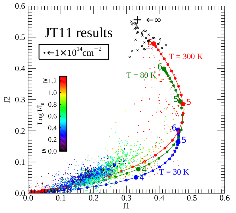
Figure 1: A depiction of pressure indicators in 2416 different radial velocity bins toward 89 stars in the survey conducted by JT11, where all measurements of $f1$ and $f2$ with uncertainties less than 0.03 are depicted by dots whose areas are proportional to $N$(C I)_total. Here, we use colors to indicate local ultraviolet starlight densities, characterized by the parameter $\log I/I_{0}$, where $I_{0}$ is the average value in our part of the Galaxy (Mathis et al. 1983). Cases where the starlight density could not be determined are shown by x marks. The curves indicate calculated outcomes for $f1$ and $f2$ for individual regions containing gas at three different temperatures, as indicated, and a range of thermal pressures indicated by dots spaced apart by 0.1 dex in $\log(p/k)$ and with numerals that signify whole-number values of $\log(p/k)~{}[{\rm cm}^{-3}$K]. The cross labeled with an $\infty$ sign is at the location where the populations are in proportion to their statistical weights, representing very high densities and temperatures.

The outcomes for the $f1$ and $f2$ results of JT11 are shown in Fig. 1, where it is evident that nearly all of the points fall above the theoretical tracks that represent homogeneous regions at a single pressure. A small percentage of the sight lines showed substantially larger contributions from high pressure gas. As noted by JT11, there were two kinds of circumstantial evidence that favored the high pressures being related to stellar environments. First, the fractional amounts of high pressure gas seemed to be driven by the intensity of starlight at the location of the gas, and second, material at predominantly negative velocities relative to expectations from differential Galactic rotation showed the best evidence of high pressures, presumably as a result of disturbances created by the target stars forcing the gas to move toward us. The relationship to starlight density is clearly illustrated by the colors of points in Fig. 1. Many of the red points in that diagram indicate that strongly irradiated gas at certain velocities show at least half of the C I in a high pressure environment.

Estimates for the column densities of neutral hydrogen $N$(H) along the sight lines in the JT11 survey could be obtained from measures of $N$(O I) or $N$(S II), and characteristic volume densities $n$(H) arise from the measurements of thermal pressures, if the temperatures are known. In turn, values of $N$(H)/$n$(H) yield an approximate longitudinal thickness of the C I-bearing gas. JT11 took such dimensions and divided them by the distances to the stars and found that most of the material occupied of order one percent of the length of the sight lines. In most cases, it is likely that this gas could be located near the target star or its association of stars, probably because it is a remaining part of a dense cloud that collapsed and led to the star formation. This consideration, along with the intensity and kinematic indications, suggests that most of the gas that was measured is situated in a region that might be subjected to disturbances such as mass loss, H II region expansion, and different forms of radiation pressure from the star or its neighbors (Lamers 2001 ; Wareing et al. 2018 ; Barnes et al. 2020 ; Ali 2021). Aside from these dynamical reasons for very high pressures, we may also consider that mild increases in pressure can arise when the enhanced radiation from stars can increase the level of heating by photoelectric emission from grains, which in turn establishes higher maximum and minimum pressures for the cold phase due to the upward shift for the thermal equilibrium curve in the representation of $\log(p/k)$ vs $\log n$(H) (Wolfire et al. 2003).

While the effects of the stars on their environments are of interest, we also wish to understand the nature of pressures in the general ISM that is well removed from the stars so that we can obtain better insights on the nature of turbulence in the general ISM. If we could observe along sight lines that did not end at stars, would we still see evidence for gas at extraordinarily high pressures? One incentive to explore this issue is a quest to see if the C I results support findings on the existence of tiny scale atomic structures (TSAS) with extraordinarily high densities. Stanimirović & Zweibel (2018) have presented a review of various investigations on the nature of TSAS, most of which arise from observations of spatial and temporal variations of 21-cm absorption (see also Rybarczyk et al. (2020)). These observations have the shortcoming that the strengths of such absorptions depend on temperatures, which are often poorly known. For any given value of $N$(H I) the C I excitations increase with temperature, while the opposite is true for 21-cm absorption. Fortunately, as one can see from the curves in Fig. 1, the outcomes for pressures based on the C I observations are not strongly dependent on temperature.

Small regions with unusually high pressures might arise from a manifestation of intermittency in turbulence, which can create shocks and provide very localized heating and compression of gas over a short time interval (Falgarone et al. 2015). Large-scale colliding flows of warm gas can create an interface that contains highly compressed small cold clouds (Audit & Hennebelle 2005 ; Vázquez-Semadeni et al. 2006), whose internal pressures may be enhanced further by self gravity (Vázquez-Semadeni et al. 2007). The more extreme cases may provide enough heating and ambipolar diffusion to facilitate the production of certain molecules that require endothermic reactions, such as CH⁺, which is formed by the ion-neutral reaction C${}^{+}+{\rm H}_{2}\rightarrow{\rm CH}^{+}+{\rm H}$ ($\Delta E/k=-4640$ K) (Draine & Katz 1986 ; Myers et al. 2015).

As a supplement to existing data on TSAS and observations of turbulent intermittency, we can examine the C I excitations, but we must use spectra from extragalactic sources of UV radiation to avoid the effects of stars. Several examples have already been published for sight lines toward the Magellanic Clouds (Nasoudi-Shoar et al. 2010 ; Welty et al. 2016). Welty et al. (2016) found the average values $f1=0.21$ and $f2=0.07$ for the Galactic velocity components in the spectra of four stars in the Magellanic Clouds, and these values are almost exactly equal to the average values found by JT11.

3 Measurements of C I toward Extragalactic Targets

Extragalactic sources are considerably fainter than the stars utilized in the JT11 survey. Nevertheless, we have identified a few cases where intensive observations yielded spectra of sufficiently good quality to warrant investigations of the C I features. All observations reported here are based on spectra recorded with the medium resolution E140M echelle mode of STIS on HST.

The Galactic coordinates, V magnitudes, and relevant velocities for C I for the selected targets are listed in Table 1. We must acknowledge that there is a selection bias toward sight lines that exhibited enough C I to measure above the noise level with some reliability. Nevertheless, our sight lines typically sample less gas than the determinations carried out in the survey by JT11, which had a median hydrogen column density of about $2\times 10^{21}{\rm cm}^{-2}$. For our Galactic latitudes that range from $23\arcdeg$ to $64\arcdeg$, we anticipate that if we use a model for the vertical distribution of H I expressed by McKee et al. (2015), our sight lines probably sample an approximate range $0.45<N$(H I)$<1.9\times 10^{21}{\rm cm}^{-2}$.

Profiles of column densities vs. velocity for the three C I levels for each sight line are shown in Fig. 2. This figure shows the velocity intervals over which we made our measurements, and these ranges are listed in Column 5 of Table 1. For the targets in the Magellanic Clouds, we have intentionally excluded the velocity ranges for absorption in these systems, since our objective is to measure C I that is not in the vicinity of the target stars.

Table 1: Targets and their C I Results

	V	Gal. Coord.		Velocity Range	Column Densities ($10^{12}{\rm cm}^{-2}[\,\rm{km\,s^{-1}}]^{-1})$
Target	mag.	$\ell$	$b$	$\,\rm{km\,s^{-1}}$(heliocentric)	$N$(C I)	$N$(C I∗)	$N$(C I∗∗)
(1)	(2)	(3)	(4)	(5)	(6)	(7)	(8)
Distant Objects
3C273 (catalog )	14.83	289.95	+64.36	12.75 to 33.75	$0.62\pm 0.05$	$0.14\pm 0.08$	$0.07\pm 0.07$
HS 0624+6907 (catalog )	14.16	145.71	+23.35	$-11.25$ to $-0.75$	$7.50\pm 0.56$	$2.97\pm 0.25$	$0.52\pm 0.25$
				0.75 to 11.25	$4.70\pm 0.39$	$0.50\pm 0.23$	$0.13\pm 0.24$
NGC 3783 (catalog )	13.43	287.45	+22.95	$-41.25$ to $-29.25$	$0.49\pm 0.04$	$0.57\pm 0.10$	$0.35\pm 0.10$
				$-11.25$ to $-2.25$	$1.26\pm 0.05$	$0.09\pm 0.11$	$0.09\pm 0.11$
				$-0.75$ to 14.25	$2.51\pm 0.05$	$1.15\pm 0.11$	$0.51\pm 0.10$
Magellanic Cloud Stars
Sk $-$67 191 (catalog )	13.44	277.66	$-$32.33	12.75 to 30.75	$1.59\pm 0.09$	$0.85\pm 0.11$	$0.19\pm 0.10$
Sk $-$68 15 (catalog )	12.69	279.52	$-$35.47	2.25 to 26.25	$2.10\pm 0.08$	$1.83\pm 0.16$	$0.63\pm 0.13$
Sk $-$69 104 (catalog )	12.10	279.92	$-$33.39	5.25 to 29.25	$1.01\pm 0.07$	$0.70\pm 0.10$	$0.18\pm 0.07$
Sk $-$71 45 (catalog )	11.55	281.86	$-$32.02	6.75 to 29.25	$1.60\pm 0.17$	$1.01\pm 0.16$	$0.12\pm 0.13$
AzV 266 (catalog )	12.61	301.90	$-$44.65	2.25 to 21.75	$1.63\pm 0.10$	$1.16\pm 0.14$	$0.47\pm 0.09$
HD 5980 (catalog )	11.31	302.07	$-$44.95	0.75 to 23.25	$1.01\pm 0.03$	$0.26\pm 0.04$	$0.08\pm 0.02$
AzV 104 (catalog )	13.22	302.91	$-$44.33	2.25 to 30.00	$1.94\pm 0.08$	$1.32\pm 0.11$	$0.58\pm 0.10$
HD 5045 (catalog )	11.04	303.01	$-$43.66	2.25 to 26.25	$1.46\pm 0.08$	$0.92\pm 0.10$	$0.36\pm 0.09$
AzV 70 (catalog )	12.40	303.05	$-$44.49	2.25 to 24.75	$2.08\pm 0.09$	$0.90\pm 0.14$	$0.28\pm 0.13$

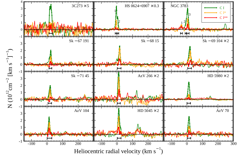
Figure 2: Derived values of column densities per unit velocity interval for C I in the three fine-structure levels as a function of heliocentric radial velocity, with colors matched to the respective levels as indicated. Displays for some targets had their amplitudes changed by uniform factors, as indicated near their identifications, to show the profiles more clearly on the uniform $y$-axis scales. Velocity intervals where the profiles were sampled are indicated by bold lines with dots on the profiles themselves and range bars at the bottom of each plot. For some targets, there were two or more such samples whose locations are indicated by numbers, and these samples are identified in separate panels in Fig. 3. Samples shown in Fig 4 had only single velocity ranges of interest. For sight lines toward the Magellanic Clouds, C I peaks that occasionally appear at $v>100\,\rm{km\,s^{-1}}$ arise from gas within the clouds, which is not relevant to our investigation. The peak at +250$\,\rm{km\,s^{-1}}$for NGC 3783 is produced by material in the high velocity cloud (HVC) 287.5+22.5+240 (aka WW187) in the leading arm of the Magellanic Stream (West et al. 1985 ; Lu et al. 1998 ; Sembach et al. 2001 ; Wakker 2001).

In our analysis of the profiles of C I, C I^∗, and C I^∗∗, we had to acknowledge the existence of two types of errors. First, there are noise fluctuations that arise from photon counting, and these errors impact the solutions for the column densities within every velocity bin. These errors become worse when the optical depths are large, which happens for some cases. In other cases, the lines are weak, and such features are affected by another source of uncertainty that is also significant. When continuum levels are not accurately determined, which is often the case for stellar targets that have very broad features in their spectra, there can be erroneous offsets in column densities that are sustained over very long intervals in velocity. These offsets are clearly evident in the tracings shown in Fig. 2, and we interpret them quantitatively by measuring them at velocities well removed from the C I absorptions.

We determine column densities for the three C I states from measurements that span many adjacent velocity bins where the contributions are visible, as indicated in Fig. 2. For the random errors arising from photon noise, we can consider that they are independent of each other from one velocity bin to the next. However, the more sustained errors from misplaced continua (i.e., long wavelength undulations) are mostly coherent over an entire measurement interval. Thus, these baseline errors can cause erroneous uniform shifts in the column densities across the complete profiles. For the observations of stellar targets, these shifts typically increased the uncertainties by a factor of two over those attributable to noise alone. For the distant objects consisting of active galactic nuclei, the spectra are more uniform with wavelength, and hence continuum errors are much smaller.

Another feature of our analysis is that when we average the column density results across a profile, we apply weight factors for the measurements in the velocity bins that are proportional $\{N$(C I$)_{\rm total}/\sigma[N$(C I$)_{\rm total}]\}^{2}$, where $\sigma[N$(C I$)_{\rm total}]$ is the uncertainty in $N$(C I$)_{\rm total}$. This weighting scheme emphasizes results near the peaks of the absorptions, which are more reliable than those near the lower amplitude wings. These weighted average column densities per unit velocity interval, along with their uncertainties, are listed in Columns 6$-$8 of Table 1.

For all of our cases, our objective is not only to determine the best values of $f1$ and $f2$, but also their uncertainties, given our expected measurement errors. The nature of these level fractions is such that the uncertainties, when large, cannot be expressed in the form of simple numerical quantities that are independent of each other. Differential probabilities in the $f1$–$f2$ space can manifest themselves in unusual shapes. In order to understand better the range of acceptable combinations of $f1$ and $f2$, we performed Markov Chain Monte Carlo (MCMC) calculations with Gibbs sampling that made successive comparisons of the $\chi^{2}$ outcomes for random trial values of $f1$, $f2$, and $N$(C I)_total. This calculation created probability densities for $f1$ and $f2$ marginalized over the quantity $N$(C I)_total, but we restricted combinations of these two variables to a region in their diagram that is physically possible for mixtures of gases at different pressures. This region is bounded by the theoretical curves on the right-hand side and a line on the left-hand side that spans between $(f1,f2)=(0,0)$ and fractions appropriate to very high temperatures and densities $(f1,f2)=(1/3,5/9)$, labeled $\infty$ in Figs. 1, 3, and 4.

4 Outcomes

Figure 3: Probability densities for $f1$ and $f2$ for C I Galactic absorption toward (a) 3C273, and (b,c) two parts of the velocity component toward HS0624+6907. Panels (d,e,f) show three velocity intervals for the results toward NGC3783.

Figure 4: Probability densities for $f1$ and $f2$ for C I Galactic absorption toward stars in the LMC (panels a-d) and SMC (panels e-i).

In this study, we have only 12 sight lines, so we do not have the vast array of measurements like those shown in Fig. 1 that were obtained by JT11, which allowed them to construct a pressure distribution function for their low pressure component. Instead, the current sample, while small, liberates us from the influence of material surrounding hot stars (although not completely, as we will describe later). The questions that we wish to answer are (1) does the distribution function of low pressure material differ from the result obtained by JT11, and (2) whether or not the small amounts of very high pressure gas seen in the JT11 survey are no longer evident or at least substantially diminished.

Figures 3 and 4 show the probability densities for $f1$ and $f2$ obtained from the MCMC analyses for our targets. The location on the diagram for Component 1 centered on $-35\,\rm{km\,s^{-1}}$ for NGC 3783 stands out markedly from the other determinations by showing a substantial fraction of the C I is at $p/k=10^{5}\,\rm{cm^{-3}K}$. Since this result clearly contrasts with the others, we will treat it as an extraordinary situation and will examine it in more detail in the following section (5.1).

5 Interpretation

5.1 The $\mathit{-35~{}km~{}s^{-1}}$ Component toward NGC 3783

As we indicated earlier, the isolated Component 1 centered at a velocity of $-35\,\rm{km\,s^{-1}}$ toward NGC 3783 showed that a substantial portion of the C I is composed of gas with a pressure of about $p/k=10^{5}\,\rm{cm^{-3}K}$ (see the lower leftmost panel in Fig. 3). However, we subsequently discovered that this anomalous outcome could be the result of two unusual conditions for this particular sight line. First, it is nearly aligned with a hot, luminous star (HD 101274, spectral type A0V, V magnitude = 9.12) with a separation of only 72$\farcs$9 from our target. This star has a Gaia EDR3 listed parallax of $2.13\pm 0.02$ mas, so the sight line passes to within about 0.166 pc of the star. The contrast between the C I for this component compared to all of the other measurements may be a confirmation of our proposition that stellar environments harbor high pressure gas. It is possible that Component 3 centered on 8$\,\rm{km\,s^{-1}}$toward this target may also be influenced by the star, since it is one of only a few cases that clearly show evidence of a small amount of high pressure material.

We estimate that from the star’s spectral type that it should have an effective temperature $T=10,000$ K and a radius of $6.76R_{\odot}$. From the stellar flux at this temperature modeled by Fossati et al. (2018), we calculate that we would need to have $n_{e}<0.06\,{\rm cm}^{-3}$ to obtain the radius of a Strömgren Sphere that extends beyond the 0.166 pc impact parameter. In our part of the Galaxy, an electron density $n_{e}\approx 0.04\,{\rm cm}^{-3}$ is a reasonable outcome for $n$(H)$=0.5\,{\rm cm}^{-3}$ (Jenkins 2013). Another possibility is that we are sensing material that has been compressed in a bow shock or thick shell caused by mass loss from the star. While mass loss rates from A0 V stars are not nearly as large as those from hotter, more luminous O- and B-type stars, they may still exhibit a strong enough outflow to create an over-pressurized shell of neutral gas (Castor et al. 1975 ; Weaver et al. 1977 ; Lancaster et al. 2021a,b). Following the finding of Beaumont et al. (2014) that such shells can be detected by their infrared emission, we examined archival Spitzer IRAC images of HD 101274 exposed at 3.6, 4.5, and $8\mu$m, but we could not see any evidence of excess emission surrounding the image of the star.

The second unusual feature of the sight line to NGC 3783 is that it penetrates an outer edge of the Antlia supernova remnant (G275.5+18.4) (McCullough et al. 2002 ; Fesen et al. 2021). As we mentioned briefly in Section 1, shocked clouds within supernova remnants are known to exhibit elevated pressures. We examined a data cube of the results from the Wisconsin H-Alpha Mapper (WHAM) (Haffner et al. 2010) in an attempt to identify the radial velocity of the H$\alpha$ emission in the general location of NGC 3783, but we found that the shell was visible over a range $-35<v_{\odot}<+35\,\rm{km\,s^{-1}}$, which precludes our being able to make a unique identification among our three chosen C I velocity intervals for the material within the SNR interior.

5.2 A General Comparison with the Results of JT11

Figure 5: Comparisons of the cumulative distribution functions for our sample (red) and those of JT11 (black) for $\log(p/k)_{\rm low}$ belonging to the dominant, low pressure fractions of C I (panels (a) and (b)), and the relative amounts $g_{\rm low}$ of C I in this component (panels (c) and (d)). Panels (a) and (c) show comparisons with the mean values for the different sight lines listed in Table 3 of JT11, while panels (b) and (d) compare our results against the multitude of narrow velocity channels shown in Table 4 in that study. In each panel we specify two quantities: (1) the maximum deviation in the vertical direction between the two distributions and (2) the resulting K-S test probabilities that the two outcomes are drawn from a single distribution.

For the reasons that we have just stated, we have elected to exclude the sight line toward NGC 3783. Of the remaining results, for each case we can interpret a representative $\log(p/k)_{\rm low}$ of the majority of the C I atoms, along with their fraction of the total $g_{\rm low}$ at these low pressures. Table 2 summarizes our results for these two quantities. We identify the remaining $1-g_{\rm low}$ amount of gas in terms of high pressure contributions that are less well defined but still considerably above the low pressure range ($p/k<20,000\,\rm{cm^{-3}K}$).

Table 2: Outcomes from the Level Populations

Target	$\log(p/k)_{\rm low}$	$g_{\rm low}$
Distant Objects
3C273 (catalog )	3.5	0.910
HS 0624+6907 (catalog )	3.8	1.00
	3.15	0.944
Magellanic Cloud Stars
Sk $-$67 191 (catalog )	4.0	1.00
Sk $-$68 15 (catalog )	4.2	0.930
Sk $-$69 104 (catalog )	4.12	1.00
Sk $-$71 45 (catalog )	4.05	1.00
AzV 266 (catalog )	4.05	0.861
HD 5980 (catalog )	3.55	0.936
AzV 104 (catalog )	4.00	0.826
HD 5045 (catalog )	4.00	0.870
AzV 70 (catalog )	3.83	0.950

Our main goal is to ascertain if there is any difference between the results obtained in this study and those derived by JT11. An effective way to compare the two and assess whether or not they differ in a statistically significant manner is to apply a Kolmogorov-Smirnov (K-S) test on relevant combinations of two cumulative distribution functions. Before doing so, we must recognize that there are differences between the way we measured pressures and the methods employed by JT11. JT11 presented the measurements of $\log(p/k)_{\rm low}$ and $g_{\rm low}$ in two forms: one was a weighted mean of the quantities of the two variables over all velocities for a given line of sight, as listed in their Table 3, while the other was a set of explicit outcomes in individual velocity channels having widths of only $0.5\,\rm{km\,s^{-1}}$ (Table 4). Our analysis may be regarded as being intermediate between these approaches: for some sight lines we isolated velocity intervals where significant changes seemed to occur and analyzed them separately, but we always evaluated weighted means of the results over moderately wide velocity intervals to increase the accuracy of the outcomes, as we show in Column 5 of Table 1. Since our approach does not exactly match the ones of JT11, we will compare our outcomes to both of those defined by JT11.

The results of the K-S tests are shown in Fig. 5. We conclude that the cumulative distribution of the results for $\log(p/k)_{\rm low}$ in our study is significantly different from both of the two measurement outcomes of JT11. The behavior of the distributions indicates a prevalence of somewhat higher pressures in our survey. For the relative proportions of high and low pressure gas, represented by distributions of $g_{\rm low}$, the differences in the distributions are not significant.

If we examine the cases displayed in Fig. 4, there is a suggestion that $g_{\rm low}$ is close to 100% for the Galactic gas in front of the LMC (panels a-d in the figure), while for the SMC this quantity averages slightly less than 90% (remaining panels). We cannot identify any reason why this should be so, other than the existence of natural changes from one region of the sky to the next, and moreover the number of cases may be too small to claim that the effect is real.

6 Discussion and Conclusions

After considering the preliminary remarks that we stated in Section 2, it is evident that our comparison of sight lines away from stars and those toward them yielded an unexpected result. Before conducting the present survey, we had anticipated that the pressures found by JT11 toward early-type stars might be somewhat higher than those that were along sight lines that avoided such stars. Instead, we found the opposite to be true. Hence the present survey indicates that the distribution of $\log(p/k)_{\rm low}$ found in the study of JT11 was not appreciably influenced by various possible forms of pressure enhancement near the stars. This conclusion does not apply to the relatively small number of cases where the starlight density is clearly far above the average value with $g_{\rm low}\lesssim 0.5$ (i.e., the red points shown in Fig. 1).

A different issue is our comparison of $g_{\rm low}$ for the two surveys. While the significance levels for the two distributions being different from each other are quite poor from the perspective of a K-S test, the figures appear to indicate that over a range $0.85<g_{\rm low}<0.95$ the cumulative distribution for the current results shows a marginally faster rise, which indicates that about 60% of our cases show a slightly larger contribution from very high pressure gas. The proposition that the high pressure contributions are about the same as or perhaps slightly higher than what JT11 found reinforces the findings from 21-cm absorption studies that there are small regions (TSAS) with extraordinarily high densities and pressures in the general interstellar medium.

We must express an important caveat about the meaning of the significance levels of the K-S tests and the apparent differences in the cumulative distributions depicted in Fig. 5. Our sample does not represent truly random directions in the sky. The Magellanic Cloud observations are tightly grouped, with many separations of order or less than one degree within in each cloud. If the coherence lengths for $\log(p/k)$ or $g_{\rm low}$ are predominantly larger than these separations, the observations should not be independent of each other. This condition will weaken the significance levels. Unfortunately, we were unable to obtain a more diverse sample of sightlines by identifying in the public archive additional AGN or QSO spectra that showed measurable C I features recorded by the STIS echelle spectrograph. While observations by the Cosmic Origins Spectrograph (COS) on HST exist for many extragalactic targets, the lower resolution and broad wings of the COS line spread function preclude our obtaining reliable results for the C I absorptions.

Finally, we reiterate a point that we made in Section 3, which is that the sight lines in the current survey sample less gas than those generally represented by the measurements of JT11. This difference may explain why we see slightly higher pressures. For both surveys, the sight lines penetrate the outer boundary of the Local Bubble, an irregular void in the cool gas that is approximately centered on our location and which has a radius of about 100 pc (Lallement et al. 2013 ; Liu et al. 2017). This bubble is believed to have been created by multiple supernova explosions over a period of about $2-15$ Myr ago (Fuchs et al. 2006 ; Schulreich et al. 2018). Its boundary may consist of an arrangement of clouds or shells holding cool gas at somewhat elevated thermal pressures (Kim et al. 2017). Because the present survey samples less gas overall, the material at the Local Bubble boundary could conceivably have a greater influence on our results compared to the samples in the survey conducted by JT11.

References

- (1) Ali, A. A. 2021, MNRAS, 501, 4136
- (2) Audit, E., & Hennebelle, P. 2005, A&A, 433, 1
- (3) Balashev, S. A., Ledoux, C., Noterdaeme, P., et al. 2020, MNRAS, 497, 1946
- (4) Barnes, A. T., Longmore, S. N., Dale, J. E., et al. 2020, MNRAS, 498, 4906
- (5) Beaumont, C. N., Goodman, A. A., Kendrew, S., Williams, J. P., & Simpson, R. 2014, ApJS, 214, 3
- (6) Boulares, A., & Cox, D. P. 1990, ApJ, 365, 544
- (7) Carswell, R. F., Jorgenson, R. A., Wolfe, A. M., & Murphy, M. T. 2011, MNRAS, 411, 2319
- (8) Castor, J. C., McCray, R., & Weaver, R. 1975, ApJ, 200, L107
- (9) Draine, B. T., & Katz, N. 1986, ApJ, 310, 392
- (10) Falgarone, E., Momferratos, G., & Lesaffre, P. 2015, in Magnetic Fields in Diffuse Media, ed. A. Lazarian (Berlin: Springer), 227
- (11) Federrath, C. 2013, MNRAS, 436, 1245
- (12) Fesen, R. A., Drechsler, M., Weil, K. E., et al. 2021, arXiv: 2102.12599
- (13) Field, G. B. 1965, ApJ, 142, 531
- (14) Field, G. B., Goldsmith, D. W., & Habing, H. J. 1969, ApJ, 155, L149
- (15) Fossati, L., Koskinen, T., Lothringer, J. D., et al. 2018, ApJ, 868, L30
- (16) Fuchs, B., Breitschwerdt, D., de Avillez, M. A., Dettbarn, C., & Flynn, C. 2006, MNRAS, 373, 993
- (17) Gazol, A. 2014, ApJ, 789, 38
- (18) Geyer, M., & Walker, M. A. 2018, MNRAS, 481, 1609
- (19) Haffner, L. M., Dettmar, R. J., Beckman, J. E., et al. 2009, RvMP, 81, 969
- (20) Haffner, L. M., Reynolds, R. J., Madsen, G. J., et al. 2010, in The Dynamic Interstellar Medium: A Celebration of the Canadian Galactic Plane Survey, eds. R. Kothes, et al.,438 (Astr. Soc. Pacific), 388
- (21) Jenkins, E. B., & Shaya, E. J. 1979, ApJ, 231, 55
- (22) Jenkins, E. B., Silk, J., Wallerstein, G., & Leep, E. M. 1981, ApJ, 248, 977
- (23) Jenkins, E. B., Jura, M., & Loewenstein, M. 1983, ApJ, 270, 88
- (24) Jenkins, E. B., Wallerstein, G., & Silk, J. 1984, ApJ, 278, 649
- (25) Jenkins, E. B., & Wallerstein, G. 1995, ApJ, 440, 227
- (26) Jenkins, E. B., Tripp, T. M., Fitzpatrick, E. L., et al. 1998, ApJ, 492, L147
- (27) Jenkins, E. B., & Tripp, T. M. 2001, ApJS, 137, 297
- (28) —. 2011, ApJ, 734, 65
- (29) Jenkins, E. B. 2013, ApJ, 764, 25
- (30) Jorgenson, R. A., Wolfe, A. M., & Prochaska, J. X. 2010, ApJ, 722, 460
- (31) Kim, C.-G., Ostriker, E. C., & Kim, W.-T. 2013, ApJ, 776, 1
- (32) Kim, C.-G., Ostriker, E. C., & Raileanu, R. 2017, ApJ, 834, 25
- (33) Klimenko, V. V., & Balashev, S. A. 2020, MNRAS, 498, 1531
- (34) Koyama, H., & Ostriker, E. C. 2009, ApJ, 693, 1346
- (35) Kritsuk, A. G., Ustyugov, S. D., & Norman, M. L. 2017, NJPh, 19, 065003
- (36) Lallement, R., Vergely, J.-L., Valette, B., et al. 2013, A&A, 561, A91
- (37) Lamers, H. J. G. L. M. 2001, PASP, 113, 263
- (38) Lancaster, L., Ostriker, E. C., Kim, J.-G., & Kim, C.-G. 2021a, arXiv: 2104.07691
- (39) —. 2021b, arXiv: 2104.07722
- (40) Liu, W., Chiao, M., Collier, M. R., et al. 2017, ApJ, 834, 33
- (41) Lockman, F. J., & Gehman, C. S. 1991, ApJ, 382, 182
- (42) Lu, L., Savage, B. D., Sembach, K. R., et al. 1998, AJ, 115, 162
- (43) Ma, J., Caucal, P., Noterdaeme, P., et al. 2015, MNRAS, 454, 1751
- (44) Mathis, J. S., Mezger, P. G., & Panagia, N. 1983, A&A, 128, 212
- (45) McCullough, P. R., Fields, B. D., & Pavlidou, V. A. 2002, ApJ, 576, L41
- (46) McKee, C. F., Parravano, A., & Hollenbach, D. J. 2015, ApJ, 814, 13
- (47) McKee, C. F. in The Evolution of the Interstellar Medium, ed. L. Blitz,12 (Astr. Soc. Pacific), 3-29
- (48) Meyer, D. M., Lauroesch, J. T., Peek, J. E. G., & Heiles, C. 2012, ApJ, 752, 119
- (49) Mocz, P., & Burkhart, B. 2019, ApJ, 884, L35
- (50) Myers, A., McKee, C., & Li, P. S. 2015, MNRAS, 453, 2747
- (51) Nasoudi-Shoar, S., Richter, P., de Boer, K. S., & Wakker, B. P. 2010, A&A, 520, A26
- (52) Noterdaeme, P., Petitjean, P., Ledoux, C., et al. 2010, A&A, 523, 80
- (53) Noterdaeme, P., Srianand, R., Rahmani, H., et al. 2015, A&A, 577, A24
- (54) Peek, J. E. G., Heiles, C., Peek, K. M. G., Meyer, D. M., & Lauroesch, J. T. 2011, ApJ, 735, 129
- (55) Quast, R., Baade, R., & Reimers, D. 2002, A&A, 386, 796
- (56) Ritchey, A. M., Jenkins, E. B., Federman, S. R., et al. 2020, ApJ, 897, 83
- (57) Roman-Duval, J., Jenkins, E. B., Tchernyshyov, K., et al. 2021, ApJ, 910, 95
- (58) Rybarczyk, D. R., Stanimirović, S., Zweibel, E. G., et al. 2020, ApJ, 893, 152
- (59) Schulreich, M. M., Breitschwerdt, D., Feige, J., & Dettbarn, C. 2018, Galaxies, 6, 26
- (60) Sembach, K. R., Howk, J. C., Savage, B. D., & Shull, J. M. 2001, AJ, 121, 992
- (61) Silva, A. I., & Viegas, S. M. 2002, MNRAS, 329, 135
- (62) Spitzer, L. 1990, ARA&A, 28, 71
- (63) Srianand, R., Petitjean, P., Ledoux, C., Ferland, G., & Shaw, G. 2005, MNRAS, 362, 549
- (64) Stanimirović, S., & Zweibel, E. G. 2018, ARA&A, 56, 489
- (65) Vázquez-Semadeni, E., Ryu, D., Passot, T., González, R. F., & Gazol, A. 2006, ApJ, 643, 245
- (66) Vázquez-Semadeni, E., Gómez, G. C., Jappsen, A. K., et al. 2007, ApJ, 657, 870
- (67) Wakker, B. P. 2001, ApJS, 136, 463
- (68) Wareing, C. J., Pittard, J. M., Wright, N. J., & Falle, S. A. E. G. 2018, MNRAS, 475, 3598
- (69) Weaver, R., McCray, R., Castor, J., Shapiro, P., & Moore, R. 1977, ApJ, 218, 377
- (70) Welty, D. E., Lauroesch, J. T., Wong, T., & York, D. G. 2016, ApJ, 821, 118
- (71) West, K. A., Pettini, M., Penston, M. V., Blades, J. C., & Morton, D. C. 1985, MNRAS, 215, 481
- (72) Wolfire, M. G., McKee, C. F., Hollenbach, D., & Tielens, A. G. G. M. 2003, ApJ, 587, 278