Spectral gap estimates for Brownian motion on domains with sticky-reflecting boundary diffusion

Abstract

Introducing an interpolation method we estimate the spectral gap for Brownian motion on general domains with sticky-reflecting boundary diffusion associated to the first nontrivial eigenvalue for the Laplace operator with corresponding Wentzell-type boundary condition. In the manifold case our proofs involve novel applications of the celebrated Reilly formula.

1 Introduction and statement of main results

Brownian motion on smooth domains with sticky-reflecting diffusion along the boundary has a long history, dating back at least to Wentzell [34]. As a prototype consider a diffusion on the closure $\overline{\Omega}$ of a smooth domain $\Omega$ with Feller generator $(\mathcal{D}(A),A)$

$$\mathcal{D}(A)=\{f\in C_{0}(\overline{\Omega})\,|\,Af\in C_{0}(\overline{\Omega})\}$$ (1.1)

$$Af=\Delta f\mathbb{I}_{\Omega}+(\beta\Delta^{\tau}f-\gamma\frac{\partial f}{\partial\nu})\mathbb{I}_{\partial\Omega}$$

where $\frac{\partial}{\partial\nu}$ is the outer normal derivative, $\Delta^{\tau}$ is the Laplace-Beltrami operator on the boundary $\partial\Omega$ and $\beta>0,\gamma\in\mathbb{R}$. The case of pure sticky reflection but no diffusion along the boundary corresponds to the regime $\beta=0$; models with $\beta>0$ have appeared recently in interacting particle systems with singular boundary or zero-range pair interaction [1, 7, 13, 19, 27]. The first rigorous process constructions on special domains $\Omega$ were given in [16, 33, 37] and were later extended to jump-diffusion processes on general domains [6] cf. [32]. An efficient construction in symmetric cases was given by Grothaus and Voßhall via Dirichlet forms in [15]. Qualitative regularity properties of the associated semigroups were studied e.g. in [14]. In this note we address the problem of estimating the spectral gap for such processes, which is a natural question also in algorithmic applications. To our knowledge this question has been considered only for $\beta=0$ by Kennedy [17] and Shouman [30]. However, for $\beta>0$ the properties of the process change significantly, which is indicated by the fact that the energy form of $A$ now also contains a boundary part and which also constitutes the main difference to the closely related work [18].

In the sequel we treat the case when $\gamma>0$ which corresponds to an inward sticky reflection at $\partial\Omega$. Our ansatz to estimate the spectral gap is based on a simple interpolation idea. To this aim assume that $\Omega$ and $\partial\Omega$ have finite (Hausdorff) measure so that we may choose $\alpha\in(0,1)$ for which

$$\frac{\alpha}{1-\alpha}\frac{|\partial\Omega|}{|\Omega|}=\gamma.$$

Introducing $\lambda_{\Omega}$ and $\lambda_{\partial}$ as normalized volume and Hausdorff measures on $\Omega$ and $\partial\Omega$ and setting

$$\lambda_{\alpha}=\alpha\lambda_{\Omega}+(1-\alpha)\lambda_{\partial},$$

we find that $-A$ is $\lambda_{\alpha}$-symmetric with first nonzero eigenvalue/spectral gap characterized by the Rayleigh quotient

$$\sigma_{\alpha,\beta}=\inf_{\begin{subarray}{c}f\in C^{1}(\overline{\Omega})\\ \operatorname{Var}_{\lambda_{\alpha}}(f)>0\end{subarray}}\frac{\mathcal{E}_{\alpha,\beta}(f)}{\operatorname{Var}_{\lambda_{\alpha}}f},$$

where

$$\operatorname{Var}_{\lambda_{\alpha}}f=\int_{\Omega}f^{2}d\lambda_{\alpha}-\left(\int_{\Omega}fd\lambda_{\alpha}\right)^{2}$$

and

$$\mathcal{E}_{\alpha,\beta}(f)=\alpha\int_{\Omega}\|\nabla f\|^{2}d\lambda_{\Omega}+(1-\alpha)\int_{\partial\Omega}\beta\|\nabla^{\tau}f\|^{2}d\lambda_{\partial},$$

and $\nabla^{\tau}$ denotes the tangential derivative operator on $\partial\Omega$.

This representation of $\sigma_{\alpha,\beta}$ formally interpolates between the two extremal cases of the spectral gap for reflecting Brownian motion on $\Omega$ when $\alpha=1$ and for Brownian motion on the surface $\partial\Omega$ when $\alpha=0$. As our main result, in Proposition 2.1 we propose a simple method to estimate $\sigma_{\alpha,\beta}$ from below using only $\sigma_{0}$ and $\sigma_{1}$ and estimates for certain bulk-boundary interaction terms which are independent of $\alpha$. The method can lead to quite good results which is illustrated by the example when $\Omega=B_{1}\subset\mathbb{R}^{d}$ is a $d$-dimensional unit ball. When $d=2$ and $\beta=1$, for instance, it yields the estimate

$$\sigma_{\alpha}\geq\frac{8(1+\alpha)\sigma_{\Omega}}{8(1-\alpha)\sigma_{\Omega}+16\alpha+3\alpha(1-\alpha)\sigma_{\Omega}}\mbox{ with }\alpha=\frac{\gamma}{2+\gamma},$$

where $\sigma_{0}\approx 3.39$ is the spectral gap for the Neumann Laplacian on the 2-dimensional unit ball, c.f.  Section 3.1. – In case when $\Omega$ is a $d$-dimensional manifold with Ricci curvature bounded from below by $k_{R}>0$ and with boundary $\partial\Omega$ whose second fundamental form $\mathop{\rm II}_{\partial\Omega}$ is bounded from below by $k_{2}>0$ we obtain (again with $\beta=1$, for simplicity) that

$$\sigma_{\alpha}\geq\min\left(\frac{dk_{R}}{C_{\Omega}dk_{R}+(1-\alpha)(d-1)},\frac{dk_{R}}{C_{\partial\Omega}}\frac{2(1-\alpha)+\alpha k_{2}C_{\partial\Omega}}{2(1-\alpha)dk_{R}+\alpha dk_{2}k_{R}C_{\Omega}+\alpha(1-\alpha)(d-1)k_{2}}\right),$$

where $C_{\Omega}$ and $C_{\partial\Omega}$ are the usual (Neumann) Poincaré constants of $\Omega$ and $\partial\Omega$ respectively. To derive this result we combine Escobar’s lower bound [9] on the first Steklov eigenvalue [12, 20] of $\Omega$ with a novel estimate on the optimal zero mean trace Poincaré constant of $\Omega$ [22, 26], for which we obtain that

$$\int_{\Omega}f^{2}dx\leq\frac{d-1}{dk_{R}}\int_{\Omega}|\nabla f|^{2},$$

for all $f\in C^{1}(\Omega)$ with $\int_{\partial\Omega}fdS=0$, and which is of independent interest. The proof is based on a novel application of Reilly’s formula [28] which is also used for a complementary lower bound of $\sigma$ independent of the interpolation approach stating that

$$\sigma_{\alpha}\geq\min\left(\frac{dk_{2}}{3d-1}\frac{\alpha}{1-\alpha}\frac{|\partial\Omega|}{|\Omega|},\frac{d}{d-1}k_{R}\right),$$

but which is generally weaker for small values of $\alpha$, c.f. Section 3.2.

The interpolation approach also yields a sufficient condition for the continuity of $\sigma_{\alpha}$ at $\alpha\in\{0,1\}$, which in general may fail. In Section 2.2 we present sufficient conditions for continuity and discontinuity of $\sigma_{\alpha}$ at $\{0,1\}$ which hints towards a phase transition in the associated family of variational problems.

We conclude with the discussion of two applications of the method in non-standard or singular situations, c.f. Sections 3.3 and 3.4.

2 An interpolation approach

2.1 Generalized framework

It will be convenient to work with a slight generalisation of the setup above. To this aim let $\Omega$ be an open domain in $\mathbb{R}^{d}$ or a Riemannian manifold with a piecewise smooth boundary $\partial\Omega$. Let $\Sigma$ be a smooth compact and connected subset of $\partial\Omega$. We denote by $\partial\Sigma$ the boundary of $\Sigma$ in the space $\partial\Omega$, i.e. $\partial\Sigma=\Sigma\cap\overline{\partial\Omega\backslash\Sigma}$. We consider two probability measures $\lambda_{\Omega}$ and $\lambda_{\Sigma}$ with support $\Omega$ and $\Sigma$, which are absolutely continuous with respect to the Lebesgue and the Hausdorff measure on $\Omega$ and $\Sigma$, respectively.

Let $\mathop{D}:C^{1}(\Omega)\mapsto\Gamma^{0}(\Omega)$ and ${\mathop{D}}^{\tau}:C^{1}(\partial\Omega)\mapsto\Gamma^{0}(\partial\Omega)$ denote given first order gradient operators mapping differentiable functions into (tangential) vector fields on $\Omega$ and on $\partial\Omega$, respectively, and for $\alpha\in[0,1]$ let

$$\lambda_{\alpha} :=\alpha\lambda_{\Omega}+(1-\alpha)\lambda_{\Sigma},$$

$$\mathcal{E}_{\alpha}(f) :=\alpha\int_{\Omega}\|\mathop{D}f\|^{2}d\lambda_{\Omega}+(1-\alpha)\int_{\Sigma}\|{\mathop{D}}^{\tau}f\|^{2}d\lambda_{\Sigma},\quad f\in\mathcal{D}_{0},$$

where $\mathcal{D}_{0}\subset\mathcal{C}^{1}(\overline{\Omega})$ is dense in $C_{0}(\Omega)$. We assume that for $\alpha\in[0,1]$ the quadratic form $(\mathcal{E}_{\alpha},\mathcal{D}_{0})$ is a pre-Dirichlet form on $L^{2}(\overline{\Omega},\lambda_{\alpha})$ whose closure we shall denote by $(\mathcal{E}_{\alpha},\mathcal{D})$, c.f. [15] for details. We wish to estimate from above $\sigma_{\alpha}^{-1}=C_{\alpha}$, where $C_{\alpha}$ is the optimal Poincaré constant given by

$$C_{\alpha}:=\sup_{\begin{subarray}{c}f\in\mathcal{D}_{0}\\ \mathcal{E}_{\alpha}(f)>0\end{subarray}}\frac{\operatorname{Var}_{\lambda_{\alpha}}f}{\mathcal{E}_{\alpha}(f)}.$$ (2.1)

In the interpolation method presented below it is assumed that $C_{\alpha}$ are known or can be estimated at the two extremals $\alpha\in\{0,1\}$. For instance, when $\mathop{D}=\nabla$, ${\mathop{D}}^{\tau}=\nabla^{\tau}$ are the standard gradient resp. tangential gradient operators and $\lambda_{\Omega}$ and $\lambda_{\Sigma}$ are normalized Lebesgue resp. Hausdorff measures on $\Omega$ and $\Sigma\subset\partial\Omega$, $C_{\Omega}:=C_{1}$ is the optimal Poincaré constant associated to the Laplace operator on $\Omega$ with Neumann boundary conditions, whereas $C_{\Sigma}:=C_{0}$ is the optimal Poincaré constant associated to the Laplace-Beltrami operator on $\Sigma$ with Neumann boundary conditions on $\partial\Sigma$.

The following proposition establishes an estimate of $C_{\alpha}$ in terms of $C_{\Omega}$ and $C_{\Sigma}$.

Proposition 2.1.

Assume there exists constants $K_{\Sigma,\Omega}$, $K_{1},K_{2}$ such that for any $f\in\mathcal{D}_{0}$

$$\operatorname{Var}_{\lambda_{\Sigma}}f\leq K_{\Sigma,\Omega}\int_{\Omega}\|\mathop{D}f\|^{2}d\lambda_{\Omega},$$ (2.2)

and

$$\left(\int_{\Omega}fd\lambda_{\Omega}-\int_{\Sigma}fd\lambda_{\Sigma}\right)^{2}\leq K_{1}\int_{\Omega}\|\mathop{D}f\|^{2}d\lambda_{\Omega}+K_{2}\int_{\Sigma}\|{\mathop{D}}^{\tau}f\|^{2}d\lambda_{\Sigma},$$ (2.3)

then it holds for any $\alpha\in(0,1)$,

$$C_{\alpha}\leq\max\left(C_{\Omega}+(1-\alpha)K_{1},\alpha K_{2},\frac{(1-\alpha)K_{\Sigma,\Omega}C_{\Sigma}+\alpha C_{\Omega}C_{\Sigma}+\alpha(1-\alpha)(K_{\Sigma,\Omega}K_{2}+C_{\Sigma}K_{1})}{(1-\alpha)K_{\Sigma,\Omega}+\alpha C_{\Sigma}}\right).$$ (2.4)

Proof.

By definition of $C_{\Sigma}$ and by (2.2), for any $f\in\mathcal{D}_{0}$

$$\operatorname{Var}_{\lambda_{\Sigma}}f\leq tK_{\Sigma,\Omega}\int_{\Omega}\|\mathop{D}f\|^{2}d\lambda_{\Omega}+(1-t)C_{\Sigma}\int_{\Sigma}\|{\mathop{D}}^{\tau}f\|^{2}d\lambda_{\Sigma},$$

for any $t\in[0,1]$. Let $\alpha\in(0,1)$. For any $f\in\mathcal{D}_{0}$ and any $t\in[0,1]$

$$\operatorname{Var}_{\lambda_{\alpha}}f =\alpha\operatorname{Var}_{\lambda_{\Omega}}f+(1-\alpha)\operatorname{Var}_{\lambda_{\Sigma}}f+\alpha(1-\alpha)\left(\int_{\Omega}fd\lambda_{\Omega}-\int_{\Sigma}fd\lambda_{\Sigma}\right)^{2}$$

$$\leq\left(C_{\Omega}+\frac{(1-\alpha)t}{\alpha}K_{\Sigma,\Omega}+(1-\alpha)K_{1}\right)\alpha\int_{\Omega}\|\mathop{D}f\|^{2}d\lambda_{\Omega}$$

$$\quad+\left((1-t)C_{\Sigma}+\alpha K_{2}\right)(1-\alpha)\int_{\Sigma}\|{\mathop{D}}^{\tau}f\|^{2}d\lambda_{\Sigma}.$$

Therefore,

$$C_{\alpha}\leq\inf_{t\in[0,1]}\max\left(C_{\Omega}+\frac{(1-\alpha)t}{\alpha}K_{\Sigma,\Omega}+(1-\alpha)K_{1},(1-t)C_{\Sigma}+\alpha K_{2}\right).$$

For any positive constants $a,b,c,d$, we have

$$\inf_{t\in[0,1]}\max\left(a+bt,c-dt\right)=\begin{cases}a&\text{if }c-a<0,\\ c-d&\text{if }c-a>b+d,\\ \frac{bc+ad}{b+d}&\text{if }0\leq c-a\leq b+d.\end{cases}$$

Therefore

$$C_{\alpha}\leq\begin{cases}C_{\Omega}+(1-\alpha)K_{1}&\text{\ \ if }\alpha K_{2}-(1-\alpha)K_{1}+C_{\Sigma}-C_{\Omega}<0,\\ \alpha K_{2}&\text{\ \ if }\alpha K_{2}-(1-\alpha)K_{1}-C_{\Omega}>\frac{1-\alpha}{\alpha}K_{\Sigma,\Omega},\\ \frac{(1-\alpha)K_{\Sigma,\Omega}C_{\Sigma}+\alpha C_{\Omega}C_{\Sigma}+\alpha(1-\alpha)(K_{\Sigma,\Omega}K_{2}+C_{\Sigma}K_{1})}{(1-\alpha)K_{\Sigma,\Omega}+\alpha C_{\Sigma}}&\begin{array}[]{r}\text{if }0\leq\alpha K_{2}-(1-\alpha)K_{1}+C_{\Sigma}-C_{\Omega}\\ \leq C_{\Sigma}+\frac{1-\alpha}{\alpha}K_{\Sigma,\Omega}.\end{array}\end{cases}$$

The last term is equivalent to the announced result. ∎

2.2 Continuity of $C_{\alpha}$

In general, the function $\alpha\mapsto C_{\alpha}$ might have discontinuities at $\alpha\in\{0,1\}$ in which cases an upper bound for $C_{\alpha}$ which interpolates continuously between $C_{0}$ and $C_{1}$ cannot exist. For example, when $\Omega=(0,b)\times(0,1)\subset\mathbb{R}^{2}$ and $\Sigma=[0,b]\times\{0\}$, straightforward computations yield

$$\lim_{\alpha\to 0}C_{\alpha}=\max\left\{C_{\Sigma},\frac{4}{\pi^{2}}\right\},$$

where $C_{\Sigma}=\frac{b^{2}}{\pi^{2}}$. Hence $\alpha\mapsto C_{\alpha}$ is discontinuous at $\alpha=0$ if and only if $b<2$. – To generalize this to the framework of Section 2.1 let $\mathcal{C}^{1}_{0}(\overline{\Omega})=\{f\in\mathcal{C}^{1}(\overline{\Omega}):f=0\mbox{ on }\Sigma\}$ and

$$\tilde{C}_{0}:=\sup_{\begin{subarray}{c}f\in\mathcal{C}^{1}_{0}(\overline{\Omega})\\ f\text{ non constant}\end{subarray}}\frac{\int_{\Omega}f^{2}d\lambda_{\Omega}}{\int_{\Omega}\|\mathop{D}f\|^{2}d\lambda_{\Omega}}.$$

(If $\mathop{D}=\nabla$, $\tilde{C}_{0}$ is the inverse of the spectral gap for Brownian motion on $\Omega$ with killing on $\Sigma$ and normal reflection at $\partial\Omega\setminus\Sigma$. ) We can then record the following statement as a partial corollary to Proposition 2.1.

Proposition 2.2.

In the setting of proposition 2.1 it holds that

$$\varliminf_{\alpha\to 0}C_{\alpha}\geq\tilde{C}_{0}.$$

In particular, if $C_{\Sigma}<\tilde{C}_{0}$, then $\alpha\mapsto C_{\alpha}$ is discontinuous at $\alpha=0$. Conversely, if $C_{\Sigma}\geq C_{\Omega}+K_{1}$ then $\alpha\mapsto C_{\alpha}$ is continuous at 0. If $C_{\Omega}\geq K_{2}$ continuity at 1 holds.

Proof.

To prove the second statement, take a non constant function $g\in\mathcal{C}^{1}_{0}(\overline{\Omega})$ and estimate

$$\varliminf_{\alpha\to 0}C_{\alpha} =\varliminf_{\alpha\to 0}\sup_{\begin{subarray}{c}f\in\mathcal{C}^{1}(\overline{\Omega})\\ f\text{ non constant}\end{subarray}}\frac{\operatorname{Var}_{\lambda_{\alpha}}f}{\mathcal{E}_{\alpha}(f)}\geq\varliminf_{\alpha\to 0}\frac{\operatorname{Var}_{\lambda_{\alpha}}g}{\mathcal{E}_{\alpha}(g)}$$

$$=\varliminf_{\alpha\to 0}\frac{\alpha\operatorname{Var}_{\lambda_{\Omega}}g+(1-\alpha)\operatorname{Var}_{\lambda_{\Sigma}}g+\alpha(1-\alpha)\left(\int_{\Omega}gd\lambda_{\Omega}-\int_{\Sigma}gd\lambda_{\Sigma}\right)^{2}}{\alpha\int_{\Omega}\|\mathop{D}g\|^{2}d\lambda_{\Omega}+(1-\alpha)\int_{\Sigma}\|{\mathop{D}}^{\tau}g\|^{2}d\lambda_{\Sigma}}.$$

Since $g=0$ on $\Sigma$, we obtain

$$\varliminf_{\alpha\to 0}C_{\alpha} \geq\varliminf_{\alpha\to 0}\frac{\alpha\operatorname{Var}_{\lambda_{\Omega}}g+\alpha(1-\alpha)\left(\int_{\Omega}gd\lambda_{\Omega}\right)^{2}}{\alpha\int_{\Omega}\|\mathop{D}g\|^{2}d\lambda_{\Omega}}=\frac{\int_{\Omega}g^{2}d\lambda_{\Omega}}{\int_{\Omega}\|\mathop{D}g\|^{2}d\lambda_{\Omega}}.$$

Taking the supremum over $g\in\mathcal{C}^{1}_{0}(\overline{\Omega})$ yields the first statement.

To prove the second assertion note that $\alpha\mapsto C_{\alpha}$ is the pointwise supremum of a family of continuous functions and therefore lower semi continuous. Thus $C_{\Sigma}=C_{0}\leq\varliminf_{\alpha\to 0}C_{\alpha}$. If $C_{\Sigma}\geq C_{\Omega}+K_{1}$, the r.h.s. of inequality (2.4) converges to $C_{\Sigma}$ as $\alpha$ goes to 0, which implies that $\varlimsup_{\alpha\to 0}C_{\alpha}\leq C_{\Sigma}$. Similarly, if $C_{\Omega}\geq K_{2}$, the r.h.s. of (2.4) converges to $C_{\Omega}$ as $\alpha$ goes ∎

Remark 2.3.

For smooth enough boundary the constant $K_{2}$ can always be taken equal to zero, hence by proposition 2.2 continuity at $\alpha=1$ holds. An example where a phase transition appears at $\alpha=0$ is given in section 3.3. In section 3.4 we present an example where $C_{\Omega}<K_{2}$ but continuity of at $\alpha=1$ can be established via Mosco-convergence [23] of the associated Dirichlet forms, see also [24].

3 Examples

3.1 Brownian motion on balls with sticky boundary diffusion

As our first example let $\Omega:=B_{1}$ be the unit ball in $\mathbb{R}^{d}$, $\Sigma=\partial\Omega$ and $\mathop{D}=\nabla$ and ${\mathop{D}}^{\tau}=\sqrt{\beta}\,\nabla^{\tau}$ with $\mathcal{D}_{0}=C^{1}(\overline{\Omega})$.

Proposition 3.1.

In the case when $\Omega=B_{1}\subset\mathbb{R}^{d}$ the optimal Poincaré constant of the generator (1.1) is bounded from above by

$$C_{\alpha}\leq\max\left(C_{\Omega}+(1-\alpha)\frac{d+1}{4d^{2}},\frac{4(1-\alpha)d+4\alpha d^{2}C_{\Omega}+\alpha(1-\alpha)(d+1)}{4d(\alpha d+(1-\alpha)\beta(d-1))}\right),$$ (3.1)

where $\alpha=\frac{\gamma}{d+\gamma}$ and $C_{\Omega}$ is the optimal Poincaré constant for reflecting Brownian motion on $B_{1}\subset\mathbb{R}^{d}$.

Proof.

In order to apply Proposition 2.1, it is sufficient to compute the constants $C_{\Sigma}$, $K_{\Sigma,\Omega}$, $K_{1}$ and $K_{2}$. We claim that inequalities (2.2) and (2.3) holds with

$$C_{\Sigma}=\frac{1}{\beta(d-1)},\quad K_{\Sigma,\Omega}=\frac{1}{d},\quad K_{1}=\frac{d+1}{4d^{2}},\quad K_{2}=0.$$

First, according to [31, Theorem 22.1], the first eigenvalue of the Laplace-Beltrami operator on the unit sphere of dimension $d-1$ is equal to $d-1$, thus $C_{\Sigma}=\frac{1}{\beta(d-1)}$.

Moreover, according to [3, Theorem 4], for every $f\in\mathcal{C}^{1}(\partial\Omega)$ one has

$$\left(\int_{\partial\Omega}|f|^{q}d\lambda_{\Sigma}\right)^{\frac{2}{q}}\leq\frac{q-2}{d}\int_{\Omega}\|\nabla u\|^{2}d\lambda_{\Omega}+\int_{\partial\Omega}f^{2}d\lambda_{\Sigma},$$

for $2\leq q<\infty$ if $d=2$ and $2\leq q<\frac{2d-2}{d-2}$ if $d\geq 3$, where $u$ is the harmonic extension of $f$ to the unit ball $\Omega$. It implies the logarithmic Sobolev inequality $\operatorname{Ent}_{\lambda_{\Sigma}}(f^{2})\leq\frac{2}{d}\int_{\Omega}\|\nabla u\|^{2}d\lambda_{\Omega}$. Repeating the proof of Proposition 5.1.3 in [2], we get $\operatorname{Var}_{\lambda_{\Sigma}}f\leq\frac{1}{d}\int_{\Omega}\|\nabla u\|^{2}d\lambda_{\Omega}$. Moreover, since the harmonic extension of $f$ is minimizing the energy functional $\mathcal{E}_{1}$ under any function with boundary condition $f$, the last inequality implies for any $f\in\mathcal{C}^{1}(\overline{\Omega})$

$$\operatorname{Var}_{\lambda_{\Sigma}}f\leq\frac{1}{d}\int_{\Omega}\|\nabla f\|^{2}d\lambda_{\Omega},$$ (3.2)

which implies $K_{\Sigma,\Omega}=\frac{1}{d}$.

Furthermore, note that $\int_{\partial\Omega}f(y)\lambda_{\Sigma}(dy)=\int_{\Omega}f(\pi_{x})\lambda_{\Omega}(dx)$, where $\pi_{x}=\frac{x}{\|x\|}$, $x\not=0$. Hence, using Jensen’s inequality and polar coordinates

$$\left(\int_{\Omega}fd\lambda_{\Omega}-\int_{\partial\Omega}fd\lambda_{\Sigma}\right)^{2} \leq\int_{\Omega}(f(x)-f(\pi_{x}))^{2}\lambda_{\Omega}(dx)$$

$$=\frac{1}{|\Omega|}\int_{\partial\Omega}\int_{0}^{1}\left(f(ry)-f(y)\right)^{2}r^{d-1}drdy$$

$$=\frac{1}{|\Omega|}\int_{\partial\Omega}\int_{0}^{1}\left(\int_{r}^{1}\frac{d}{ds}f(sy)ds\right)^{2}r^{d-1}drdy$$

$$\leq\frac{1}{|\Omega|}\int_{\partial\Omega}\int_{0}^{1}(1-r)\left(\int_{r}^{1}\left(\frac{d}{ds}f(sy)\right)^{2}ds\right)r^{d-1}drdy$$

$$=\frac{1}{|\Omega|}\int_{\partial\Omega}\int_{0}^{1}\left[\int_{0}^{s}(1-r)r^{d-1}dr\right]\left(\frac{d}{ds}f(sy)\right)^{2}dsdy.$$

We separately estimate

$$\int_{0}^{s}(1-r)r^{d-1}dr=\left(\frac{s}{d}-\frac{s^{2}}{d+1}\right)s^{d-1}\leq\frac{d+1}{4d^{2}}s^{d-1}.$$

for any $s\in[0,1]$. Hence,

$$\left(\int_{\Omega}fd\lambda_{\Omega}-\int_{\partial\Omega}fd\lambda_{\Sigma}\right)^{2} \leq\frac{d+1}{4d^{2}|\Omega|}\int_{\partial\Omega}\int_{0}^{1}\left(\nabla f(sy)\cdot y\right)^{2}s^{d-1}ds$$

$$=\frac{d+1}{4d^{2}|\Omega|}\int_{\partial\Omega}\int_{0}^{1}\left\|\nabla f(sy)\right\|^{2}s^{d-1}dsdy$$

$$=\frac{d+1}{4d^{2}}\int_{\Omega}\|\nabla f(x)\|^{2}\lambda_{\Omega}(dx).$$ (3.3)

which implies $K_{1}=\frac{d+1}{4d^{2}}$ and $K_{2}=0$. ∎

For illustration, in $d=2,$ we compare the bound from Proposition 3.1 for $\beta=1,\gamma>0$ to the optimal constant $C_{\alpha}$ which will be computed numerically. To evaluate the bound (3.1), note that in this case

$$C_{\Omega}=\frac{1}{\sigma_{\Omega}}\approx\frac{1}{3.39},$$ (3.4)

where $\sigma_{\Omega}$ is the smallest positive eigenvalue of the Laplace operator with Neumann boundary condition on the circle. It is given as the minimal positive solution to the equation $J_{m}^{\prime}(\sqrt{\gamma})=0$, $m\in\mathbb{N}_{0}$, where $J_{m}$ is the Bessel function of the first kind of parameter $m$, defined by $J_{m}(x)=\frac{1}{\pi}\int_{0}^{\pi}\cos(mt-x\sin t)dt$, $x\geq 0$. As a consequence, inequality (3.1) becomes

$$C_{\alpha}\leq\frac{8(1-\alpha)\sigma_{\Omega}+16\alpha+3\alpha(1-\alpha)\sigma_{\Omega}}{8(1+\alpha)\sigma_{\Omega}}.$$ (3.5)

For the numerical computation of $C_{\alpha}$ one notes that the generator $A_{\alpha}$ associated with $\mathcal{E}_{\alpha}$ is defined on $D(A_{\alpha})\subset\mathcal{C}^{2}(\overline{\Omega})$ as

$$A_{\alpha}f=\mathbb{I}_{\Omega}\Delta f+\mathbb{I}_{\partial\Omega}\left(\Delta^{\tau}f-\frac{2\alpha}{1-\alpha}\frac{\partial f}{\partial\nu}\right),$$

where $\Delta^{\tau}$ and $\frac{\partial}{\partial\nu}$ denote the Laplace-Beltrami operator and the outer normal derivative on the circle $\partial\Omega$. Hence, an eigenvector of $-A_{\alpha}$ for eigenvalue $\lambda\geq 0$ is a function $f\in D(A_{\alpha})$ such that

$$A_{\alpha}f=-\lambda f\quad\mbox{in}\ \ \Omega.$$

This equation is equivalent to the system of partial differential equations

$$\begin{cases}\Delta f=-\lambda f&\mbox{in}\ \ \Omega,\\ \Delta^{\tau}f-\frac{2\alpha}{1-\alpha}\frac{\partial f}{\partial\nu}=-\lambda f&\mbox{on}\ \ \partial\Omega,\end{cases}$$

which by the continuity of $f$ can be rewritten as

$$\begin{cases}\Delta f=-\lambda f&\mbox{in}\ \ \Omega,\\ \Delta f=\Delta^{\tau}f-\frac{2\alpha}{1-\alpha}\frac{\partial f}{\partial\nu}&\mbox{on}\ \ \partial\Omega.\end{cases}$$

Passing to polar coordinates $(x_{1},x_{2})=(r\cos\theta,r\sin\theta)\in\Omega$ in $d=2$ and separating variables, we obtain the set of eigenfunctions $\{f_{m,l}^{c},f_{m,l}^{s}\}_{m,l\in\mathbb{N}_{0}}$,

$$f_{m,l}^{c}(x_{1},x_{2})=J_{m}(\sqrt{\lambda_{m,l}}r)\cos(m\theta),\quad m,l\in\mathbb{N}_{0},$$

$$f_{m,l}^{s}(x_{1},x_{2})=J_{m}(\sqrt{\lambda_{m,l}}r)\sin(m\theta),\quad m\in\mathbb{N},\ \ l\in\mathbb{N}_{0},$$

where $\lambda_{m,l}$, $l\in\mathbb{N}_{0}$, are countable family of positive solutions to the equation

$$\sqrt{\lambda}J_{m}^{\prime\prime}(\sqrt{\lambda})+\frac{1+\alpha}{1-\alpha}J_{m}^{\prime}(\sqrt{\lambda})=0$$ (3.6)

for every $m\in\mathbb{N}_{0}$. Since the family $\{f_{m,l}^{c},\ m,l\in\mathbb{N}_{0}\}\cup\{f_{m,l}^{s},\ m\in\mathbb{N}_{0},\ l\in\mathbb{N}_{0}\}$ is dense in $L_{2}(\Omega,\lambda_{\alpha})$ and the operator $A_{\alpha}$ is symmetric, the standard argument implies

$$C_{\alpha}=\frac{1}{\lambda_{\alpha,\star}},$$ (3.7)

where $\lambda_{\alpha,\star}=\min\limits_{m,l\in\mathbb{N}_{0}}\lambda_{m,l}$. The resulting curves are plotted in Figure 1.

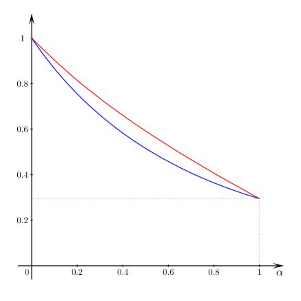
Figure 1: The blue curve represents $\alpha\mapsto C_{\alpha}$ the optimal Poincaré constant when $\Omega$ is the unit ball of $\mathbb{R}^{2}$ with full boundary diffusion. The red curve is the upper estimate given by (3.5).

3.2 Smooth manifold with boundary

Let $\Omega$ be a smooth compact Riemannian manifold of dimension $d$ with piecewise smooth boundary $\partial\Omega$. We denote by $\operatorname{Ric}$ the Ricci curvature of $\Omega$ and by $\mathrm{II}$ the second fundamental form on the boundary $\partial\Omega$. Assume in this section that:

$$\text{Assumption (M)}:\quad\quad\quad\quad\quad\exists k_{r}>0,k_{2}>0,\quad\operatorname{Ric}|_{\Omega}\geq k_{R}\operatorname{id}\quad\text{and}\quad\mathrm{II}|_{\partial\Omega}\geq k_{2}\operatorname{id}.$$

As before we consider $\Sigma=\partial\Omega$, $\mathop{D}=\nabla$ and ${\mathop{D}}^{\tau}=\nabla^{\tau}$ with $\mathcal{D}_{0}=C^{1}(\overline{\Omega})$.

Proposition 3.2.

Under assumption (M), it holds that

$$C_{\alpha}\leq\max\left(C_{\Omega}+\frac{(1-\alpha)(d-1)}{dk_{R}},\frac{C_{\Sigma}}{dk_{R}}\cdot\frac{2(1-\alpha)dk_{R}+\alpha dk_{2}k_{R}C_{\Omega}+\alpha(1-\alpha)(d-1)k_{2}}{2(1-\alpha)+\alpha k_{2}C_{\Sigma}}\right)=:M_{1}.$$ (3.8)

This statement is obtained via Proposition 2.1 and the two statements below.

Proposition 3.3.

Under assumption (M), inequality (2.3) is satisfied with $K_{2}=0$ and

$$K_{1}=\frac{d-1}{dk_{R}}.$$

Proof.

Our goal is to obtain an lower bound of

$$\inf_{\begin{subarray}{c}f\in C^{1}(\overline{\Omega})\end{subarray}}\frac{\int_{\Omega}\|\nabla f\|^{2}d\lambda_{\Omega}}{\left(\int_{\Omega}fd\lambda_{\Omega}-\int_{\Sigma}fd\lambda_{\Sigma}\right)^{2}},$$

where we recall that $\Sigma=\partial\Omega$. We note that

$$\inf_{\begin{subarray}{c}f\in C^{1}(\overline{\Omega})\end{subarray}}\frac{\int_{\Omega}\|\nabla f\|^{2}d\lambda_{\Omega}}{\left(\int_{\Omega}fd\lambda_{\Omega}-\int_{\Sigma}fd\lambda_{\Sigma}\right)^{2}}=\inf_{\begin{subarray}{c}f\in C^{1}(\overline{\Omega})\\ \int_{\Sigma}fd\lambda_{\Sigma}=0\end{subarray}}\frac{\int_{\Omega}\|\nabla f\|^{2}d\lambda_{\Omega}}{\left(\int_{\Omega}fd\lambda_{\Omega}\right)^{2}}\geq\inf_{\begin{subarray}{c}f\in C^{1}(\overline{\Omega})\\ \int_{\Sigma}fd\lambda_{\Sigma}=0\end{subarray}}\frac{\int_{\Omega}\|\nabla f\|^{2}d\lambda_{\Omega}}{\int_{\Omega}f^{2}d\lambda_{\Omega}}=:\sigma.$$

Let $f\in C^{1}(\overline{\Omega})$ be a minimizer for $\sigma$. Then $\int_{\Sigma}fd\lambda_{\Sigma}=0$ and

$$\int_{\Omega}\nabla f\cdot\nabla\xi d\lambda_{\Omega}=\sigma\int_{\Omega}f\xi d\lambda_{\Omega}$$

for each $\xi\in C^{1}(\overline{\Omega})$ with $\int_{\Sigma}\xi d\lambda_{\Sigma}=0$. By integration by parts, the latter equality is equivalent to

$$-\int_{\Omega}\Delta f\xi d\lambda_{\Omega}+\frac{|\Sigma|}{|\Omega|}\int_{\Sigma}\frac{\partial f}{\partial\nu}\xi d\lambda_{\Sigma}=\sigma\int_{\Omega}f\xi d\lambda_{\Omega}$$

for each $\xi\in C^{1}(\overline{\Omega})$ satisfying $\int_{\Sigma}\xi d\lambda_{\Sigma}=0$. In particular, choosing $\xi\in C^{\infty}_{0}(\Omega)$ (which obviously satisfies $\int_{\Sigma}\xi d\lambda_{\Sigma}=0$), we get that $f$ should satisfy $-\Delta f=\sigma f$ in $\Omega$. Hence $\int_{\Sigma}\frac{\partial f}{\partial\nu}\xi d\lambda_{\Sigma}=0$ for each $\xi$ with zero mean, so it follows that $\int_{\Sigma}\frac{\partial f}{\partial\nu}\left(\xi-\int_{\Sigma}\xi d\lambda_{\Sigma}\right)d\lambda_{\Sigma}=0$ for every $\xi\in C^{1}(\overline{\Omega})$, which is equivalent to

$$\int_{\Sigma}\left(\frac{\partial f}{\partial\nu}-\int_{\Sigma}\frac{\partial f}{\partial\nu}d\lambda_{\Sigma}\right)\xi d\lambda_{\Sigma}=0$$

for every $\xi\in C^{1}(\overline{\Omega})$. It follows that $\frac{\partial f}{\partial\nu}$ is constant on $\Sigma$. Therefore, $f$ satisfies

$$\begin{cases}\Delta f=-\sigma f&\mbox{in}\ \ \Omega,\\ \frac{\partial f}{\partial\nu}\equiv c&\mbox{on}\ \ \partial\Omega,\\ \int_{\Sigma}fd\lambda_{\Sigma}=0,\end{cases}$$ (3.9)

for some constant $c$.

Moreover, recall Reilly’s formula (see [28])

$$\int_{\Omega}\left((\Delta f)^{2}-\|\nabla^{2}f\|^{2}\right)dx =\int_{\Omega}\operatorname{Ric}(\nabla f,\nabla f)dx$$ (3.10)

$$\quad+\int_{\Sigma}\left(H(\frac{\partial f}{\partial\nu})^{2}+\mathrm{II}(\nabla^{\tau}f,\nabla^{\tau}f)+2\Delta^{\tau}f\frac{\partial f}{\partial\nu}\right)dS$$

where $dx$ and $dS$ denote the Riemannian volume resp. surface measure on $\Omega$ and $\partial\Omega$, $\nabla^{2}f$ is the Hessian of $f$ and $H$ is the mean curvature of $\Sigma$ (i.e. the trace of $\mathrm{II}$). Since $f$ satisfies (3.9),

$$\int_{\Omega}(\Delta f)^{2}dx=-\sigma\int_{\Omega}f\Delta fdx =\sigma\int_{\Omega}\|\nabla f\|^{2}dx-\sigma\int_{\Sigma}\frac{\partial f}{\partial\nu}fdS$$

$$=\sigma\int_{\Omega}\|\nabla f\|^{2}dx-\sigma c\int_{\Sigma}fdS=\sigma\int_{\Omega}\|\nabla f\|^{2}dx,$$

because $\int_{\Sigma}fdS=|\Sigma|\int_{\Sigma}fd\lambda_{\Sigma}=0$. Furthermore, note that $\|\nabla^{2}f\|^{2}=\sum_{i,j}(\partial_{ij}^{2}f)^{2}\geq\sum_{i=1}^{d}(\partial_{ii}^{2}f)^{2}\geq\frac{1}{d}(\sum_{i=1}^{d}\partial_{ii}^{2}f)^{2}=\frac{1}{d}(\Delta f)^{2}$. Therefore, the l.h.s. of (3.10) is bounded by

$$\int_{\Omega}\left((\Delta f)^{2}-\|\nabla^{2}f\|^{2}\right)dx\leq\frac{d-1}{d}\int_{\Omega}(\Delta f)^{2}dx\leq\frac{d-1}{d}\sigma\int_{\Omega}\|\nabla f\|^{2}dx.$$

On the other hand, by assumption (M), $H\geq 0$, $\mathrm{II}(\nabla^{\tau}f,\nabla^{\tau}f)\geq 0$ and

$$\int_{\Omega}\operatorname{Ric}(\nabla f,\nabla f)dx\geq k_{R}\int_{\Omega}\|\nabla f\|^{2}dx.$$

Since

$$\int_{\Sigma}\Delta^{\tau}f\frac{\partial f}{\partial\nu}dS=c\int_{\Sigma}\Delta^{\tau}fdS=0$$

the r.h.s. of (3.10) is bounded from below by $k_{R}\int_{\Omega}\|\nabla f\|^{2}dx$. It turns out that

$$\frac{d-1}{d}\sigma\int_{\Omega}\|\nabla f\|^{2}dx\geq k_{R}\int_{\Omega}\|\nabla f\|^{2}dx,$$

which implies that $\sigma\geq\frac{d}{d-1}k_{R}$. It follows that inequality (2.3) holds with $K_{1}=\frac{d-1}{dk_{R}}$. ∎

Remark 3.4.

Instead of using $K_{1}$ from Proposition 3.3 another admissible choice is

$$K_{1}^{\prime}=\frac{|\Omega|}{|\partial\Omega|}B^{2}(1+C_{\Omega})<\infty,$$

where $B$ is the optimal Sobolev trace constant of $\Omega$, i.e. the norm of the embedding $H^{1,2}(\Omega)\hookrightarrow L^{2}(\partial\Omega)$. $B^{-2}$ is the first nontrivial eigenvalue of a Steklov-type eigenvalue problem

$$\begin{cases}-\Delta f+f=0&\mbox{ in }\Omega\\ \frac{\partial f}{\partial\nu}=\sigma f&\mbox{ on }\partial\Omega,\end{cases}$$

for which however explicit lower bounds in terms of the geometry of $\Omega$ seem yet unknown [4, 5, 11, 21, 29].

Proposition 3.5.

Under assumption (M), inequality (2.2) holds with $K_{\Sigma,\Omega}=\frac{2}{k_{2}}$.

Proof.

The optimal choice for $K_{\Sigma,\Omega}$ is $\sigma^{-1}$, where $\sigma$ given by

$$\sigma=\inf_{\begin{subarray}{c}f\in C^{1}(\overline{\Omega})\\ \int_{\Sigma}fd\lambda_{\Sigma}=0\end{subarray}}\frac{\int_{\Omega}\|\nabla f\|^{2}d\lambda_{\Omega}}{\left(\int_{\Sigma}f^{2}d\lambda_{\Sigma}\right)^{2}}$$

is the first nontrivial eigenvalue of the Steklov-problem c.f. [12]

$$\begin{cases}\Delta f=0&\mbox{ in }\Omega,\\ \frac{\partial f}{\partial\nu}=\sigma f&\mbox{ on }\partial\Omega.\end{cases}$$

Escobar [9] showed $\sigma\geq\frac{k_{2}}{2}$ in this case. ∎

Alternatively, we obtain another upper bound for $C_{\alpha}$ by a direct application of Reilly’s formula.

Proposition 3.6.

Under assumption (M) it holds that

$$C_{\alpha}\leq\max\left(\frac{(3d-1)(1-\alpha)}{d\alpha k_{2}}\frac{|\Omega|}{|\partial\Omega|},\frac{d-1}{dk_{R}}\right)=:M_{2}.$$ (3.11)

Proof.

We estimate equivalently from below the first nontrivial eigenvalue $\sigma=C_{\alpha}^{-1}$ for the problem

$$\begin{cases}\Delta f+\sigma f=0&\mbox{ in }\Omega\\ \Delta^{\tau}f-\gamma\frac{\partial f}{\partial\nu}+\sigma f=0&\mbox{ on }\partial\Omega,\end{cases}$$

where $\gamma=\frac{\alpha}{1-\alpha}\frac{|\partial\Omega|}{|\Omega|}$. As in the proof of Proposition 3.3 we apply Reilly’s formula (3.10) to the corresponding eigenfunction $f$. In this case, for the l.h.s. we estimae

$$\int_{\Omega}\left((\Delta f)^{2}-\|\nabla^{2}f\|^{2}\right)dx \leq\frac{d-1}{d}\int_{\Omega}(\Delta f)^{2}dx=-\frac{d-1}{d}\sigma\int_{\Omega}f\Delta fdx$$

$$=\frac{d-1}{d}\sigma\int_{\Omega}\|\nabla f\|^{2}dx-\frac{d-1}{d}\sigma\int_{\Sigma}\frac{\partial f}{\partial\nu}fdS$$

$$=\frac{d-1}{d}\sigma\int_{\Omega}\|\nabla f\|^{2}dx-\frac{d-1}{d}\frac{\sigma}{\gamma}\int_{\Sigma}(\Delta^{\tau}f+{\sigma}f)fdS$$

$$=\frac{d-1}{d}\sigma\int_{\Omega}\|\nabla f\|^{2}dx+\frac{d-1}{d}\frac{\sigma}{\gamma}\int_{\Sigma}\|\nabla^{\tau}f\|^{2}dS-\frac{d-1}{d}\frac{\sigma^{2}}{\gamma}\int_{\Sigma}f^{2}dS$$

$$\leq\frac{d-1}{d}\sigma\int_{\Omega}\|\nabla f\|^{2}dx+\frac{d-1}{d}\frac{\sigma}{\gamma}\int_{\Sigma}\|\nabla^{\tau}f\|^{2}dS.$$

Since

$$\int_{\Sigma}\frac{\partial f}{\partial\nu}\Delta^{\tau}fdS =\frac{1}{\gamma}\int_{\Sigma}(\Delta^{\tau}f+\sigma f)\Delta^{\tau}fdS$$

$$=\frac{1}{\gamma}\int_{\Sigma}(\Delta^{\tau}f)^{2}dS-\frac{\sigma}{\gamma}\int_{\Sigma}\|\nabla^{\tau}f\|^{2}dS\geq-\frac{\sigma}{\gamma}\int_{\Sigma}\|\nabla^{\tau}f\|^{2}dS$$

the r.h.s. of (3.10) is bounded from below by

$$k_{R}\int_{\Omega}\|\nabla f\|^{2}dx -\frac{2\sigma}{\gamma}\int_{\Sigma}\|\nabla^{\tau}f\|^{2}dS+\int_{\Sigma}h|\frac{\partial f}{\partial\nu}|^{2}dS+k_{2}\int_{\Sigma}\|\nabla^{\tau}f\|^{2}dS$$

$$\geq k_{R}\int_{\Omega}\|\nabla f\|^{2}dx-\frac{2\sigma}{\gamma}\int_{\Sigma}\|\nabla^{\tau}f\|^{2}dS+k_{2}\int_{\Sigma}\|\nabla^{\tau}f\|^{2}dS.$$

Combining the two bounds for (3.10) yields

$$\left(\frac{d-1}{d}\sigma-k_{R}\right)\int_{\Omega}\|\nabla f\|^{2}dx\geq\left(k_{2}-\frac{3d-1}{d}\frac{\sigma}{\gamma}\right)\int_{\Sigma}\|\nabla^{\tau}f\|^{2}dS,$$

which implies that either

$$k_{2}-\frac{3d-1}{d}\frac{\sigma}{\gamma}\leq 0,\quad\mbox{ i.e. }\quad\sigma\geq\frac{dk_{2}\gamma}{3d-1}$$

or

$$\frac{d-1}{d}\sigma-k_{R}\geq 0,\quad\mbox{ i.e. }\quad\sigma\geq\frac{d}{d-1}k_{r}.$$

Consequently,

$$\sigma\geq\min\left(\frac{dk_{2}\gamma}{3d-1},\frac{d}{d-1}k_{R}\right).$$

∎

Corollary 3.7.

Under assumption (M), it holds that

$$C_{\alpha}\leq\min(M_{1},M_{2}),$$

where $M_{1}=M_{1}(\alpha)$ and $M_{2}=M_{2}(\alpha)$ are defined by (3.8) and (3.11), respectively.

When $\alpha$ goes to 0, $M_{1}$ tends to $\max(C_{\Omega},\frac{d-1}{dk_{R}},C_{\Sigma})$ and $M_{2}$ tends to $+\infty$, so the estimation via the interpolation method is always stronger. When $\alpha$ goes to $1$, $M_{1}$ tends to $C_{\Omega}$ and $M_{2}$ tends to $\frac{d-1}{dk_{R}}$, so the relative strength of each method depends on the values of $C_{\Omega}$, $d$ and $k_{R}$.

3.3 Brownian motion on balls with partial sticky reflecting boundary diffusion

As in Section 3.1, let $\Omega:=B_{1}$ be the unit ball of $\mathbb{R}^{2}$. Now, define for a fixed $\delta\in(0,1)$

$$\Sigma=\{(\cos\theta,\sin\theta)\in\partial\Omega:-\delta\pi\leq\theta\leq\delta\pi\},\quad\quad\Sigma_{\operatorname{N}}:=\partial\Omega\backslash\Sigma.$$

Proposition 3.8.

It holds that

$$C_{\alpha}\leq\max\left(C_{\Omega}+(1-\alpha)K_{1}(\delta),\frac{4(1-\alpha)\delta^{2}+8\alpha\delta^{3}C_{\Omega}+8\alpha(1-\alpha)\delta^{3}K_{1}(\delta)}{(1-\alpha)+8\alpha\delta^{3}}\right),$$ (3.12)

where $C_{\Omega}=\frac{1}{\sigma_{\Omega}}\approx\frac{1}{3.39}$ and $K_{1}(\delta)=\left(\sqrt{1-\delta}\pi+\frac{1}{4}\sqrt{\frac{3}{\delta}}\right)^{2}$.

As previously, we will start by computing the needed constants $C_{\Omega}$, $C_{\Sigma}$, $K_{\Sigma,\Omega}$, $K_{1}$ and $K_{2}$. The first constant, $C_{\Omega}=\frac{1}{\sigma_{\Omega}}\approx\frac{1}{3.39}$, remains unchanged.

Lemma 3.9.

The following inequalities hold true

$$\operatorname{Var}_{\lambda_{\Sigma}}f \leq C_{\Sigma}\int_{\Sigma}\|\nabla^{\tau}f\|^{2}d\lambda_{\Sigma},$$ (3.13)

$$\operatorname{Var}_{\lambda_{\Sigma}}f \leq K_{\Sigma,\Omega}\int_{\Omega}\|\nabla f\|^{2}d\lambda_{\Omega},$$ (3.14)

where $C_{\Sigma}=4\delta^{2}$ and $K_{\Sigma,\Omega}=\frac{1}{2\delta}$.

Proof.

Inequality (3.13) corresponds to the Poincaré inequality of the Laplacian on the one-dimensional interval $[-\delta\pi,\delta\pi]$ with Neumann boundary conditions. It is well known (see [2, Prop. 4.5.5]) that the optimal Poincaré constant is given by $C_{\Sigma}=4\delta^{2}$.

Moreover, let us decompose the normalized Hausdorff measure $\lambda_{\partial}$ on the sphere $\partial\Omega$ into the normalized Hausdorff measure $\lambda_{\Sigma}$ on $\Sigma$ and the normalized Hausdorff measure $\lambda_{\operatorname{N}}$ on $\Sigma_{\operatorname{N}}$: $\lambda_{\partial}=\delta\lambda_{\Sigma}+(1-\delta)\lambda_{\operatorname{N}}$. Therefore

$$\operatorname{Var}_{\lambda_{\partial}}f=\delta\operatorname{Var}_{\lambda_{\Sigma}}f+(1-\delta)\operatorname{Var}_{\lambda_{\operatorname{N}}}f+\delta(1-\delta)\left(\int_{\Sigma}fd\lambda_{\Sigma}-\int_{\Sigma_{\operatorname{N}}}fd\lambda_{\operatorname{N}}\right)^{2}\geq\delta\operatorname{Var}_{\lambda_{\Sigma}}f,$$

Furthermore, recall that by inequality (3.2), for any $f\in\mathcal{C}^{1}(\overline{\Omega})$, $\operatorname{Var}_{\lambda_{\partial}}f\leq\frac{1}{2}\int_{\Omega}\|\nabla f\|^{2}d\lambda_{\Omega}$. It implies (3.14). ∎

Lemma 3.10.

It holds that

$$\left(\int_{\Omega}fd\lambda_{\Omega}-\int_{\Sigma}fd\lambda_{\Sigma}\right)^{2}\leq K_{1}(\delta)\int_{\Omega}\|\nabla f\|^{2}d\lambda_{\Omega}$$

with $K_{1}(\delta)=\left(\sqrt{1-\delta}\pi+\frac{1}{4}\sqrt{\frac{3}{\delta}}\right)^{2}$.

Proof.

For every $x\in\Omega\backslash\{0\}$ with polar coordinates $(r,\theta)$, $r\in(0,1)$, $\theta\in(-\pi,\pi]$, denote by $p_{x}$ the point of coordinates $(1,\delta\theta)$ on $\Sigma$. Obviously, $\int_{\Sigma}f(y)\lambda_{\Sigma}(dy)=\int_{\Omega}f(p_{x})\lambda_{\Omega}(dx)$ and by Jensen’s inequality

$$I:=\left(\int_{\Omega}fd\lambda_{\Omega}-\int_{\Sigma}fd\lambda_{\Sigma}\right)^{2}\leq\int_{\Omega}\left(f(x)-f(p_{x})\right)^{2}\lambda_{\Omega}(dx).$$

Define $g(r,\theta):=f(r\cos(\theta),r\sin(\theta))$. Then

$$I \leq\frac{1}{\pi}\int_{0}^{1}\int_{-\pi}^{\pi}(g(r,\theta)-g(1,\delta\theta))^{2}rdrd\theta\leq(\sqrt{J_{1}}+\sqrt{J_{2}})^{2},$$ (3.15)

where $J_{1}=\frac{1}{\pi}\int_{0}^{1}\int_{-\pi}^{\pi}(g(r,\theta)-g(r,\delta\theta))^{2}rdrd\theta$ and $J_{2}=\frac{1}{\pi}\int_{0}^{1}\int_{-\pi}^{\pi}(g(r,\delta\theta)-g(1,\delta\theta))^{2}rdrd\theta$. On the one hand

$$J_{1} =\frac{1}{\pi}\int_{0}^{1}\int_{-\pi}^{\pi}\left(\int_{\delta\theta}^{\theta}\frac{\partial g}{\partial\theta}(r,u)du\right)^{2}rdrd\theta\leq\frac{1-\delta}{\pi}\int_{0}^{1}\int_{-\pi}^{\pi}|\theta|\int_{-\pi}^{\pi}\left(\frac{\partial g}{\partial\theta}\right)^{2}(r,u)du\;rdrd\theta$$

$$\leq(1-\delta)\pi^{2}\frac{1}{\pi}\int_{0}^{1}\int_{-\pi}^{\pi}\left(\frac{1}{r}\frac{\partial g}{\partial\theta}\right)^{2}(r,u)du\;rdr\leq(1-\delta)\pi^{2}\int_{\Omega}\|\nabla f\|^{2}d\lambda_{\Omega}.$$ (3.16)

On the other hand

$$J_{2} \leq\frac{1}{\pi}\int_{0}^{1}\int_{-\pi}^{\pi}(1-r)\int_{r}^{1}\left(\frac{\partial g}{\partial r}\right)^{2}(s,\delta\theta)ds\;rdrd\theta\leq\frac{1}{\pi}\int_{0}^{1}\int_{-\pi}^{\pi}\left(\frac{\partial g}{\partial r}\right)^{2}(s,\delta\theta)\int_{0}^{s}(1-r)rdrdsd\theta.$$

For every $s\in[0,1]$, $\int_{0}^{s}(1-r)rdr=\frac{s^{2}}{2}-\frac{s^{3}}{3}\leq\frac{3s}{16}$, thus

$$J_{2} \leq\frac{3}{16\delta\pi}\int_{0}^{1}\int_{-\delta\pi}^{\delta\pi}\left(\frac{\partial g}{\partial r}\right)^{2}(s,u)sdsdu\leq\frac{3}{16\delta}\int_{\Omega}\|\nabla f\|^{2}d\lambda_{\Omega}.$$ (3.17)

The proof of the lemma is completed by putting together (3.15), (3.16) and (3.17). ∎

Proof of Proposition 3.8.

We apply Proposition 2.1 with $C_{\Omega}=\frac{1}{\sigma_{\Omega}}$, $C_{\Sigma}=4\delta^{2}$, $K_{\Sigma,\Omega}=\frac{1}{2\delta}$, $K_{1}(\delta)=\left(\sqrt{1-\delta}\pi+\frac{1}{4}\sqrt{\frac{3}{\delta}}\right)^{2}$ and $K_{2}=0$. ∎

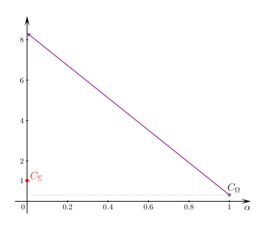
(a) $\delta=0.5$

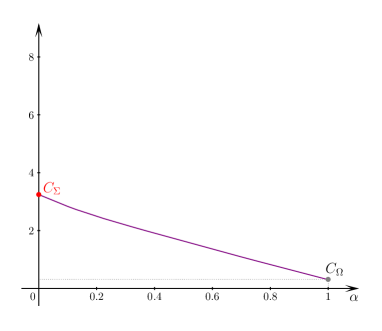
(b) $\delta=0.9$

Figure 2: The above two figures show the upper estimate given by the r.h.s of (3.12). In the case $\delta=0.9$ (Figure 2b), the curve interpolates between the extremal constants $C_{\Sigma}$ and $C_{\Omega}$, as opposed to the half-sphere case (Figure 2a).

For $\delta$ sufficiently large, the map $\alpha\mapsto C_{\alpha}$ is continuous at $\alpha=0$. Indeed, by Proposition 2.2, a sufficient condition is $C_{\Sigma}(\delta)>C_{\Omega}+K_{1}(\delta)$, that is

$$4\delta^{2}>\frac{1}{\sigma_{\Omega}}+\left(\sqrt{1-\delta}\pi+\frac{1}{4}\sqrt{\frac{3}{\delta}}\right)^{2},$$

which is satisfied for any $\delta\geq 0.862$.

3.4 Ball with a needle

Our final example is the unit ball $\Omega=B_{1}$ of $\mathbb{R}^{2}$ with a needle $\mathcal{L}$ of length $L$ attached to one point of the boundary, i.e.  $\mathcal{L}:=\{(x,0):1\leq x\leq L+1\}$, see Figure 3. The attachment point and the endpoint of the needle are denoted by $x_{0}:=(1,0)$ and $x_{L}=(L+1,0)$, respectively.

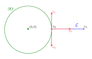
Figure 3: The ball (in green) is denoted by $\Omega$, the boundary of the ball is denoted by $\partial\Omega$ and the needle (in blue) is denoted by $\mathcal{L}$.

In that setting, we define $\overline{\Omega}=\overline{B_{1}}\cup\mathcal{L}$, $\Sigma=\partial B_{1}\cup\mathcal{L}$ and

$$\lambda_{\alpha}=\alpha\lambda_{\Omega}+(1-\alpha)\lambda_{\Sigma},$$

where $\lambda_{\Omega}$ is as previously the normalized Lebesgue measure on $\Omega$ and $\lambda_{\Sigma}=\frac{2\pi}{2\pi+L}\lambda_{\partial}+\frac{L}{2\pi+L}\lambda_{\mathcal{L}}$, with $\lambda_{\partial}$ and $\lambda_{\mathcal{L}}$ being the normalized Hausdorff measures on $\partial\Omega$ and $\mathcal{L}$, respectively. We choose

$$\mathcal{D}_{0}=\left\{f\in C_{0}(\overline{\Omega}))\cap C^{1}(\overline{\Omega}\setminus\{x_{0}\})\,|\,\frac{\partial f}{\partial e_{1}}+\frac{\partial f}{\partial e_{2}}+\frac{\partial f}{\partial e_{3}}=0\mbox{ at }x_{0}\right\},$$

where $e_{1}=(0,1)$, $e_{2}=(0,-1)$ and $e_{3}=(1,0)$ are the three ”tangent” vectors to $\Sigma$ at point $x_{0}$, and $\mathop{D}:=\nabla$, ${\mathop{D}}^{\tau}:=\sqrt{\beta}\nabla^{\tau}$, which is well defined in $\Sigma\setminus\{x_{0}\}$. With this choice, for $\alpha\in[0,1]$ $(\mathcal{E}_{\alpha},\mathcal{D}_{0})$ is a pre-Dirichlet form on $L^{2}(\overline{\Omega},\lambda_{\alpha})$, whose closure generates Brownian motion on $\Omega$ with sticky boundary diffusion on $\Sigma$, i.e. whose generator is given by

$$A_{\alpha}(f)=\Delta f\mathbb{I}_{\Omega}+\beta\Delta_{\Sigma}f\mathbb{I}_{\Sigma}-\frac{\alpha}{1-\alpha}\frac{2\pi+L}{\pi}\frac{\partial f}{\partial\nu}\mathbb{I}_{\partial\Omega},$$

with $\Delta_{\Sigma}$ being the generator of the canonical diffusion on $\Sigma$ with reflecting boundary condition at $x_{L}$. As before, the optimal Poincaré constant $C_{\alpha}$ for $A_{\alpha}$ is given by

$$C_{\alpha}:=\sup_{\begin{subarray}{c}f\in\mathcal{D}_{0}\\ \mathcal{E}_{\alpha}(f)>0\end{subarray}}\frac{\operatorname{Var}_{\lambda_{\alpha}}f}{\mathcal{E}_{\alpha}(f)},$$

and let $C_{\Omega}:=C_{1}$ and $C_{\Sigma}:=C_{0}$. In this case the following estimate is obtained.

Proposition 3.11.

$$C_{\alpha}\leq\max\left(\frac{1}{\sigma_{\Omega}}+\frac{3}{8}(1-\alpha),\frac{1}{\beta\gamma_{L}}+\alpha\frac{L^{2}(\pi+L)}{\beta(2\pi+L)}\right),$$

where $\gamma_{L}>0$ is the smallest positive solution to

$$2\cos(\sqrt{\gamma}L)(1-\cos(\sqrt{\gamma}2\pi))+\sin(\sqrt{\gamma}L)\sin(\sqrt{\gamma}2\pi)=0.$$ (3.18)

Note that $\gamma_{L}\leq 1$ for any $L>0$ and if $L=2\pi$, $\gamma_{2\pi}=\left(\frac{\arccos(-1/3)}{2\pi}\right)^{2}\approx 0.0925$.

Let us compute the constants needed to apply Proposition 2.1. As we do not expect an inequality of type (2.2) to hold in that case, we set $K_{\Sigma,\Omega}:=+\infty$. Moreover, $C_{\Sigma}$ can be computed exactly as follows.

Lemma 3.12.

In this case, $C_{\Sigma}=\frac{1}{\beta\gamma_{L}}$.

Proof.

The constant $\frac{1}{C_{\Sigma}}$ is the smallest non-zero eigenvalue $\gamma$ of the following problem:

$$\begin{cases}\beta\Delta^{\tau}f=-\gamma f&\mbox{on}\ \ \Sigma\backslash\{x_{0}\},\\ \frac{\partial f}{\partial\nu}=0&\mbox{at point }x_{L},\\ \frac{\partial f}{\partial e_{1}}+\frac{\partial f}{\partial e_{2}}+\frac{\partial f}{\partial e_{3}}=0&\mbox{at point }x_{0},\end{cases}$$

where $\Delta^{\tau}$ is the Laplace-Beltrami operator on $\partial\Omega$ and $\mathcal{L}$. A general solution to that boundary value problem is given by

$$f(x)=\begin{cases}A\cos(\sqrt{\frac{\gamma}{\beta}}y)+B\sin(\sqrt{\frac{\gamma}{\beta}}y)&\mbox{if }x=(y,0)\in\mathcal{L},\\ C\cos(\sqrt{\frac{\gamma}{\beta}}\theta)+D\sin(\sqrt{\frac{\gamma}{\beta}}\theta)&\mbox{if }x=(\cos\theta,\sin\theta)\in\partial\Omega,\end{cases}$$

where $A$, $B$, $C$ and $D$ have to satisfy the continuity assumption of $f$ at point $x_{0}$ and both boundary conditions, that is:

$$\left\{\begin{aligned} A&=C=C\cos(\sqrt{\frac{\gamma}{\beta}}2\pi)+D\sin(\sqrt{\frac{\gamma}{\beta}}2\pi),\\ 0&=-A\sin(\sqrt{\frac{\gamma}{\beta}}L)+B\cos(\sqrt{\frac{\gamma}{\beta}}L),\\ 0&=B+D+C\sin(\sqrt{\frac{\gamma}{\beta}}2\pi)-D\cos(\sqrt{\frac{\gamma}{\beta}}2\pi).\end{aligned}\right.$$

A short computation shows that this system has a non-trivial solution if and only if $\frac{\gamma}{\beta}$ solves (3.18). Therefore, $\frac{1}{C_{\Sigma}}=\beta\gamma_{L}$. Obviously, $\gamma=1$ is a solution to (3.18), thus $\gamma_{L}\leq 1$. ∎

Next, we look for the constants $K_{1}$ and $K_{2}$.

Lemma 3.13.

Inequality (2.3) holds with $K_{1}=\frac{3}{8}$ and $K_{2}=\frac{L^{2}(\pi+L)}{\beta(2\pi+L)}$.

Proof.

Recall that $\Sigma=\partial\Omega\cup\mathcal{L}$. Let us insert the average of $f$ over $\partial\Omega$ as follows:

$$\left(\int_{\Omega}fd\lambda_{\Omega}-\int_{\Sigma}fd\lambda_{\Sigma}\right)^{2} \leq 2\left(\int_{\Omega}fd\lambda_{\Omega}-\int_{\partial\Omega}fd\lambda_{\partial}\right)^{2}+2\left(\int_{\partial\Omega}fd\lambda_{\partial}-\int_{\Sigma}fd\lambda_{\Sigma}\right)^{2}$$

$$\leq\frac{3}{8}\int_{\Omega}\|\nabla f\|^{2}d\lambda_{\Omega}+2\left(\int_{\partial\Omega}fd\lambda_{\partial}-\int_{\Sigma}fd\lambda_{\Sigma}\right)^{2},$$

where the second inequality follows directly from (3.3). Moreover, recalling that $\lambda_{\Sigma}=\frac{2\pi}{2\pi+L}\lambda_{\partial}+\frac{L}{2\pi+L}\lambda_{\mathcal{L}}$

$$\left(\int_{\partial\Omega}fd\lambda_{\partial}-\int_{\Sigma}fd\lambda_{\Sigma}\right)^{2} =\frac{L^{2}}{(2\pi+L)^{2}}\left(\int_{\partial\Omega}fd\lambda_{\partial}-\int_{\mathcal{L}}fd\lambda_{\mathcal{L}}\right)^{2}.$$

For every $x=(\cos\theta,\sin\theta)\in\partial\Omega$, with $\theta\in(-\pi,\pi]$, we denote by $p_{x}$ the point of $\mathcal{L}$ with coordinates $(1+L-\frac{|\theta|L}{\pi},0)$. It follows that

$$\left(\int_{\partial\Omega}fd\lambda_{\partial}-\int_{\mathcal{L}}fd\lambda_{\mathcal{L}}\right)^{2}=\left(\int_{\partial\Omega}(f(x)-f(p_{x}))d\lambda_{\partial}\right)^{2}\leq\int_{\partial\Omega}(f(x)-f(p_{x}))^{2}d\lambda_{\partial}.$$

Denoting by $\lambda_{\partial}^{+}$ and $\lambda_{\partial}^{-}$ the normalized Hausdorff measures on $\partial\Omega^{+}:=\{(x,y)\in\partial\Omega:y>0\}$ and $\partial\Omega^{-}:=\{(x,y)\in\partial\Omega:y<0\}$, respectively,

$$\int_{\partial\Omega}(f(x)-f(p_{x}))^{2}d\lambda_{\partial}=\frac{1}{2}\int_{\partial\Omega^{+}}(f(x)-f(p_{x}))^{2}d\lambda^{+}_{\partial}+\frac{1}{2}\int_{\partial\Omega^{-}}(f(x)-f(p_{x}))^{2}d\lambda^{-}_{\partial}.$$

Moreover, for any $\mathcal{C}^{1}$-function $g:[-\pi,L]\to\mathbb{R}$,

$$\frac{1}{\pi}\int_{0}^{\pi}\left|g(-\theta)-g(L-\textstyle\frac{\theta L}{\pi})\right|^{2}d\theta\leq\frac{\pi+L}{2}\int_{-\pi}^{L}|g^{\prime}(t)|^{2}dt,$$

so we deduce, identifying $\partial\Omega^{+}$ with $[-\pi,0]$ and $\mathcal{L}$ with $[0,L]$, that

$$\int_{\partial\Omega^{+}}(f(x)-f(p_{x}))^{2}d\lambda^{+}_{\partial}\leq\frac{\pi+L}{2}\left(\pi\int_{\partial\Omega^{+}}\|\nabla^{\tau}f\|^{2}d\lambda^{+}_{\partial}+L\int_{\mathcal{L}}\|\nabla^{\tau}f\|^{2}d\lambda_{\mathcal{L}}\right)$$

and using symmetry to deal with $\partial\Omega^{-}$, we obtain

$$\int_{\partial\Omega}(f(x)-f(p_{x}))^{2}d\lambda_{\partial} \leq\frac{\pi+L}{4}\left(\pi\int_{\partial\Omega^{+}}\|\nabla^{\tau}f\|^{2}d\lambda^{+}_{\partial}+\pi\int_{\partial\Omega^{-}}\|\nabla^{\tau}f\|^{2}d\lambda^{-}_{\partial}+2L\int_{\mathcal{L}}\|\nabla^{\tau}f\|^{2}d\lambda_{\mathcal{L}}\right)$$

$$\leq\frac{(\pi+L)(2\pi+L)}{2}\int_{\Sigma}\|\nabla^{\tau}f\|^{2}d\lambda_{\Sigma}.$$

Putting together the above inequalities, we get

$$\left(\int_{\Omega}fd\lambda_{\Omega}-\int_{\Sigma}fd\lambda_{\Sigma}\right)^{2} \leq\frac{3}{8}\int_{\Omega}\|\nabla f\|^{2}d\lambda_{\Omega}+2\frac{L^{2}}{(2\pi+L)^{2}}\frac{(\pi+L)(2\pi+L)}{2\beta}\int_{\Sigma}\beta\|\nabla^{\tau}f\|^{2}d\lambda_{\Sigma}$$

which leads to inequality (2.3) with $K_{1}=\frac{3}{8}$ and $K_{2}=\frac{L^{2}(\pi+L)}{\beta(2\pi+L)}$. ∎

Proof of Proposition 3.11.

Since $K_{\Sigma,\Omega}=\infty$, we immediately get from Proposition 2.1 that

$$C_{\alpha}\leq\max\left(C_{\Omega}+(1-\alpha)K_{1},\alpha K_{2},C_{\Sigma}+\alpha K_{2}\right)=\max\left(C_{\Omega}+(1-\alpha)K_{1},C_{\Sigma}+\alpha K_{2}\right).$$

Therefore,

$$C_{\alpha}\leq\max\left(\frac{1}{\sigma_{\Omega}}+\frac{3}{8}(1-\alpha),\frac{1}{\beta\gamma_{L}}+\alpha\frac{L^{2}(\pi+L)}{\beta(2\pi+L)}\right),$$ (3.19)

where $\sigma_{\Omega}\approx 3.39$. ∎

Remark 3.14.

If $\beta$ is large enough, that is if the diffusion velocity is larger on $\Sigma$ than on $\Omega$, then the first term in (3.19) dominates. Precisely, if $\beta\geq\sigma_{\Omega}\left(\frac{1}{\gamma_{L}}+\frac{L^{2}(\pi+L)}{2\pi+L}\right)$, then (3.19) rewrites for any $\alpha$

$$C_{\alpha}\leq\frac{1}{\sigma_{\Omega}}+\frac{3}{8}(1-\alpha).$$

Conversely, if $\beta\leq\frac{1}{\gamma_{L}}\left(\frac{1}{\sigma_{\Omega}}+\frac{3}{8}\right)^{-1}$, then (3.19) rewrites for any $\alpha$

$$C_{\alpha}\leq\frac{1}{\beta\gamma_{L}}+\alpha\frac{L^{2}(\pi+L)}{\beta(2\pi+L)}.$$

References

- [1] Alexander Aurell and Boualem Djehiche, Behavior near walls in the mean-field approach to crowd dynamics, SIAM J. Appl. Math. 80 (2020), no. 3, 1153–1174. MR 4096131
- [2] Dominique Bakry, Ivan Gentil, and Michel Ledoux, Analysis and geometry of Markov diffusion operators, Grundlehren der Mathematischen Wissenschaften [Fundamental Principles of Mathematical Sciences], vol. 348, Springer, Cham, 2014. MR 3155209
- [3] William Beckner, Sharp Sobolev inequalities on the sphere and the Moser-Trudinger inequality, Ann. of Math. (2) 138 (1993), no. 1, 213–242. MR 1230930
- [4] Rodney Josué Biezuner, Best constants in Sobolev trace inequalities, Nonlinear Anal. 54 (2003), no. 3, 575–589. MR 1978428
- [5] Julián Fernández Bonder, Julio D. Rossi, and Raúl Ferreira, Uniform bounds for the best Sobolev trace constant, Adv. Nonlinear Stud. 3 (2003), no. 2, 181–192. MR 1971310
- [6] Jean-Michel Bony, Philippe Courrège, and Pierre Priouret, Semi-groupes de Feller sur une variété à bord compacte et problèmes aux limites intégro-différentiels du second ordre donnant lieu au principe du maximum, Ann. Inst. Fourier (Grenoble) 18 (1968), no. fasc. 2, 369–521 (1969). MR 245085
- [7] Jean-Dominique Deuschel, Giambattista Giacomin, and Lorenzo Zambotti, Scaling limits of equilibrium wetting models in -dimension, Probab. Theory Related Fields 132 (2005), no. 4, 471–500. MR 2198199
- [8] Klaus-Jochen Engel, The Laplacian on with generalized Wentzell boundary conditions, Arch. Math. (Basel) 81 (2003), no. 5, 548–558. MR 2029716
- [9] José F. Escobar, The geometry of the first non-zero Stekloff eigenvalue, J. Funct. Anal. 150 (1997), no. 2, 544–556. MR 1479552
- [10] Torben Fattler, Martin Grothaus, and Robert Voßhall, Construction and analysis of a sticky reflected distorted Brownian motion, Ann. Inst. Henri Poincaré Probab. Stat. 52 (2016), no. 2, 735–762. MR 3498008
- [11] Vincenzo Ferone, Carlo Nitsch, and Cristina Trombetti, On a conjectured reverse Faber-Krahn inequality for a Steklov-type Laplacian eigenvalue, Commun. Pure Appl. Anal. 14 (2015), no. 1, 63–82. MR 3299025
- [12] Alexandre Girouard and Iosif Polterovich, Spectral geometry of the Steklov problem (survey article), J. Spectr. Theory 7 (2017), no. 2, 321–359. MR 3662010
- [13] Gisèle Ruiz Goldstein, Derivation and physical interpretation of general boundary conditions, Adv. Differential Equations 11 (2006), no. 4, 457–480. MR 2215623
- [14] Gisèle Ruiz Goldstein, Jerome A. Goldstein, Davide Guidetti, and Silvia Romanelli, Maximal regularity, analytic semigroups, and dynamic and general Wentzell boundary conditions with a diffusion term on the boundary, Ann. Mat. Pura Appl. (4) 199 (2020), no. 1, 127–146. MR 4065110
- [15] Martin Grothaus and Robert Voßhall, Stochastic differential equations with sticky reflection and boundary diffusion, Electron. J. Probab. 22 (2017), Paper No. 7, 37. MR 3613700
- [16] Nobuyuki Ikeda, On the construction of two-dimensional diffusion processes satisfying Wentzell’s boundary conditions and its application to boundary value problems, Mem. Coll. Sci. Univ. Kyoto Ser. A. Math. 33 (1960/61), 367–427. MR 126883
- [17] James Kennedy, An isoperimetric inequality for the second eigenvalue of the Laplacian with Robin boundary conditions, Proc. Amer. Math. Soc. 137 (2009), no. 2, 627–633. MR 2448584
- [18] Alexander V. Kolesnikov and Emanuel Milman, Brascamp-Lieb-type inequalities on weighted Riemannian manifolds with boundary, J. Geom. Anal. 27 (2017), no. 2, 1680–1702. MR 3625169
- [19] Vitalii Konarovskyi and Max von Renesse, Reversible coalescing-fragmentating Wasserstein dynamics on the real line, 2017.
- [20] Nikolay Kuznetsov and Alexander Nazarov, Sharp constants in the Poincaré, Steklov and related inequalities (a survey), Mathematika 61 (2015), no. 2, 328–344. MR 3343056
- [21] Yanyan Li and Meijun Zhu, Sharp Sobolev trace inequalities on Riemannian manifolds with boundaries, Comm. Pure Appl. Math. 50 (1997), no. 5, 449–487. MR 1443055
- [22] Svetlana Matculevich and Sergey Repin, Explicit constants in Poincaré-type inequalities for simplicial domains and application to a posteriori estimates, Comput. Methods Appl. Math. 16 (2016), no. 2, 277–298. MR 3483617
- [23] Umberto Mosco, Composite media and asymptotic Dirichlet forms, J. Funct. Anal. 123 (1994), no. 2, 368–421. MR 1283033
- [24] Delio Mugnolo, Robin Nittka, and Olaf Post, Norm convergence of sectorial operators on varying Hilbert spaces, Oper. Matrices 7 (2013), no. 4, 955–995. MR 3154581
- [25] Delio Mugnolo and Silvia Romanelli, Dirichlet forms for general Wentzell boundary conditions, analytic semigroups, and cosine operator functions, Electron. J. Differential Equations (2006), No. 118, 20. MR 2255233
- [26] A. I. Nazarov and S. I. Repin, Exact constants in Poincaré type inequalities for functions with zero mean boundary traces, Math. Methods Appl. Sci. 38 (2015), no. 15, 3195–3207. MR 3400329
- [27] Andreas Nonnenmacher and Martin Grothaus, Overdamped limit of generalized stochastic hamiltonian systems for singular interaction potentials, 2018.
- [28] Robert C. Reilly, Applications of the Hessian operator in a Riemannian manifold, Indiana Univ. Math. J. 26 (1977), no. 3, 459–472. MR 474149
- [29] Julio D. Rossi, First variations of the best Sobolev trace constant with respect to the domain, Canad. Math. Bull. 51 (2008), no. 1, 140–145. MR 2384747
- [30] Abdolhakim Shouman, Generalization of Philippin’s results for the first Robin eigenvalue and estimates for eigenvalues of the bi-drifting Laplacian, Ann. Global Anal. Geom. 55 (2019), no. 4, 805–817. MR 3951758
- [31] M. A. Shubin, Pseudodifferential operators and spectral theory, second ed., Springer-Verlag, Berlin, 2001, Translated from the 1978 Russian original by Stig I. Andersson. MR 1852334
- [32] Kazuaki Taira, Boundary value problems and Markov processes, third ed., Lecture Notes in Mathematics, vol. 1499, Springer, Cham, [2020] ©2020, Functional analysis methods for Markov processes. MR 4176673
- [33] Satoshi Takanobu and Shinzo Watanabe, On the existence and uniqueness of diffusion processes with Wentzell’s boundary conditions, J. Math. Kyoto Univ. 28 (1988), no. 1, 71–80. MR 929208
- [34] A. D. Ventcel, On boundary conditions for multi-dimensional diffusion processes, Theor. Probability Appl. 4 (1959), 164–177. MR 121855
- [35] Hendrik Vogt and Jürgen Voigt, Wentzell boundary conditions in the context of Dirichlet forms, Adv. Differential Equations 8 (2003), no. 7, 821–842. MR 1988680
- [36] Mahamadi Warma, The Robin and Wentzell-Robin Laplacians on Lipschitz domains, Semigroup Forum 73 (2006), no. 1, 10–30. MR 2277314
- [37] Shinzo Watanabe, On stochastic differential equations for multi-dimensional diffusion processes with boundary conditions. II, J. Math. Kyoto Univ. 11 (1971), 545–551. MR 287612