Entanglement Effect and Angular Momentum Conservation in a Non-separable Tunneling Treatment

Abstract

The important, and often dominant, role of tunneling in low temperature kinetics has resulted in numerous theoretical explorations into the methodology for predicting it. Nevertheless, there are still key aspects of the derivations that are lacking, particularly for non-separable systems in the low temperature regime, and further explorations of the physical factors affecting the tunneling rate are warranted. In this work we obtain a closed-form rate expression for the tunneling rate constant that is a direct analog of the rigid-rotor-harmonic-oscillator expression. This expression introduces a novel ”entanglement factor” that modulates the reaction rate. Furthermore, we are able to extend this expression, which is valid for non-separable systems at low temperatures, to properly account for the conservation of angular momentum. In contrast, previous calculations have considered only vibrational transverse modes and so effectively employ a decoupled rotational partition function for the orientational modes. We also suggest a simple theoretical model to describe the tunneling effects in the vicinity of the crossover temperature (the temperature where tunneling becomes the dominating mechanism). This model allows one to naturally classify, interpret, and predict experimental data. Among other things, it quantitatively explains in simple terms the so-called “quantum bobsled” effect, also known as the negative centrifugal effect, which is related to curvature of the reaction path. Taken together, the expressions obtained here allow one to predict the thermal and $E$-resolved rate constants over broad ranges of temperatures and energies.

1. Introduction

The famous transition state (TS) theory high pressure rate constant expression reads¹ (we use atomic units, $\hbar=1$)

$$k=\frac{k_{B}T}{2\pi}\frac{Z^{\#}}{Z_{R}}e^{-V^{\#}/k_{B}T},$$ (1.1)

where $T$ and $k_{B}$ are temperature and the Boltzmann constant, $Z_{R}$ is the partition function of the reactant(s), and $V^{\#}$ is the barrier height. The partition function for the TS dividing surface $Z^{\#}$ can be factorized into rotational and vibrational contributions in the framework of the rigid-rotor harmonic-oscillator (RRHO) approximation at the saddle point,

$$Z^{\#} = Z^{\#}_{rot}Z^{\#}_{vib},$$ (1.2)

$$Z^{\#}_{rot} = 2\sqrt{2\pi}\sqrt{I_{x}I_{y}I_{z}}\beta^{-3/2},$$ (1.3)

$$Z^{\#}_{vib} = \prod_{i}\frac{1}{2\sinh(\omega_{i}\beta/2)},$$ (1.4)

where $\beta=1/k_{B}T$, $I_{i}$ are the principal inertia moments at the saddle point, and $\omega_{i}$ are the frequencies for motions transverse to the reaction coordinate.

Ad hoc approaches for accounting for the effects of tunneling often assume a separability between the effects of tunneling and the contribution of the transverse modes to the transition state partition function. Commonly, this assumption is implemented in terms of a separability of the reaction coordinate and the transverse modes. Then an additional tunneling factor enters into Eq. 1.2,

$$Z^{\#} = Z^{\#}_{tun}Z^{\#}_{rot}Z^{\#}_{vib},$$ (1.5)

$$Z^{\#}_{tun} = \beta\int dEP(E)e^{-\beta E},$$ (1.6)

where $P(E)$ is the one-dimensional barrier transmission coefficient at energy $E$. In the spirit of the RRHO approximation, a parabolic barrier approximation can be used, for which the tunneling transmission coefficent reads,

$$P(E)=\frac{1}{1+e^{-2\pi E/\omega_{b}}},$$ (1.7)

where $\omega_{b}$ is the imaginary frequency at the saddle point and the saddle point is taken as the zero of energy. Substituting Eq. 1.7 into Eq. 1.6 one obtains the classic Wigner tunneling expression,²

$$Z^{\#}_{tun}=\frac{\omega_{b}\beta/2}{\sin(\omega_{b}\beta/2)}.$$ (1.8)

While Eq. 1.8 takes into account local tunneling effects, it fails at low temperatures because the integral in Eq. 1.6 diverges at low energies for the parabolic barrier. This divergence occurs at temperatures lower than the crossover temperature, $T_{c}$,

$$k_{B}T_{c}=\frac{\omega_{b}}{2\pi}.$$ (1.9)

To avoid this divergence one should use a more realistic model for the transmission coefficient. In the one-dimensional WKB approximation, the transmission coefficient reads,

$$P(E)=e^{-\tilde{S}(-E)},\ E<0,$$ (1.10)

where $\tilde{S}(E)$ is the abbreviated action over the periodic trajectory along the reaction coordinate $r$ with the energy $E$ in the inverted barrier potential $-V(r)$,

$$\tilde{S}(E)=2\int_{r_{-}}^{r_{+}}dr\sqrt{2m_{r}(E+V(r))},$$ (1.11)

where $r_{\pm}$ are the left and right turning points and $m_{r}$ is the mass associated with the reaction coordinate. Evaluating the integral in Eq. 1.6 in the stationary phase approximation (SPA) one obtains,

$$Z^{\#}_{tun}=\sqrt{2\pi}\beta\left(\frac{d^{2}\tilde{S}(E)}{dE^{2}}\right)^{-1/2}e^{-\tilde{S}(E)+\beta E},\ \frac{d\tilde{S}}{dE}=\beta,$$ (1.12)

which is valid in the ”deep tunneling” regime where the Wigner expression fails.

From Eqs. 1.11 and 1.12 one can see that, in contrast with the localized TS dividing surface of relevance at higher temperatures, in the deep tunneling regime the contribution from tunneling through the TS is related to the dynamics over a relatively wide range of coordinates. As a result, in the deep tunneling regime, the separability assumption between the reaction coordinate and the transverse modes becomes questionable and it is desirable to construct a theory that avoids this assumption. Over the years, tremendous effort has been devoted to constructing such a theory. For conciseness, we review only a few results of particular relevance to our further discussion.

Long ago Langer³ suggested that the tunneling rate constant can be calculated via analytical continuation of the system partition function $Z=Z_{R}+\frac{i}{2}Z_{I}$, considered as a path integral in the configurational space of the closed paths. The imaginary part in this integral comes from the vicinity of the trajectory that corresponds to the saddle point in that space and the path integral is considered in the quadratic approximation. The TS partition function $Z^{\#}$ in Eq. 1.1 then reads,

$$Z^{\#}=2\pi Z_{I},$$ (1.13)

Affleck⁴ considered the transition from low to high temperatures for one-dimensional systems and has confirmed that Eq. 1.13 coincides with Eq. 1.12 at temperatures below the crossover.

Many prior studies focused on the evaluation of the microcanonical rate constant rather than the canonical one. Miller⁵, who was one of the pioneers in the study of muti-dimensional tunneling effects in chemical reactions, applied his correlation function formalism⁶ and Gutzwiller’s expression for the Green’s function⁷ to obtain the expression for the “cumulative reaction probability”, which we prefer to call the microcanonical number of states, $N(E)$, in the spirit of RRKM theory.⁸ Notably, it was later realized that the expression obtained for $N(E)$ did not agree with the exact expression in the separable multi-dimensional case and a correction was suggested.⁹ Curiosly enough, Miller in his original paper⁵ also suggested an expression for the thermal rate constant that is correct in the separable case but his derivation was inaccurate.¹⁰ Furthermore, as we see, this expression appears to be missing key terms of relevance to non-separable systems. Alternative, non-separable tunneling path approximations have been developed for the ground vibrational state in the framework of the vibrational adiabaticity assumption, starting with the seminal paper of Marcus and Coltrin.¹¹ Truhlar and co-wokers, who have originally developed many of these approaches,^{12, 13} extensively used them in thermal rate constant calculations.^{14, 15, 16, 17, 18, 19}

Benderskii et al.^{20, 21} further discussed the derivation of the rate constant within Langer’s approach. By neglecting the interaction between longitudinal and transverse fluctuations, they obtained an explicit expression for the rate constant that coincided with Miller’s expression for the thermal rate constant.⁵ It includes the product $1/\prod_{i}2\sinh(u_{i}/2)$ as a prefactor, which looks formally similar to the vibrational partition function, cf. Eq. 1.4. Furthermore, the stability parameters $u_{i}$, which were first introduced by Gutzwiller,^{5, 7} approach their classical values $u_{i}=\beta\omega_{i}$ when the temperature approaches $T_{c}$, making the analogy with the vibrational partition function complete. Jackels et al.²² contributed to the practical aspects of the tunneling path calculations through a potential expansion in the vicinity of the minimum energy path (MEP). Richardson^{23, 24} has used an improved Green’s function approximation within Miller’s correlation function expressions.²⁵ Many papers have successfully used the so called ring polymer molecular dynamics approach for the tunneling rate constant calculation.^{26, 27} This approach implements Langer’s theory directly by approximating the partition function path integral with a large number of beads.

To summarize, two generic classes of results are available in the literature. These two classes differ in the presumed starting point for the derivation. The papers based on Miller’s correlation function formalism express the rate constant in terms of a Boltzmann weighted integral over energy. The integrand is expressed via Green’s functions, for which different approximations are used. The advantage of this approach is that it is better justified and allows for a smooth transition from low to high temperatures. Its drawback is that current implementations do not reproduce the exact separable result, cf. Eq.1.5, because of the difficultities in evaluating the Green’s function.

On the other hand, the papers based on Langer’s approach typically either use different kinds of decoupling approximations to obtain the final rate constant or calculate the fluctuation part of the path integral directly. We did not find in the literature a closed rate expression for the non-separable reactive system. So the main goal of this paper is to provide such an expression that can be substituted for Eq. 1.5 in the deep tunneling regime. Also, all analytical papers we have seen, with one exception, do not take into account the conservation of angular momentum. The one exception is a paper by Miller⁵, which, as we will discuss later, is flawed. Therefore, the second goal of this paper is to fill this gap by providing an expression for the analog of the rotational partition function in the deep tunneling regime, and which goes smoothly to the classical rotational partition function at higher temperatures. We will also work through various ramifications of our results, focusing on perturbative expansions.

The layout of the paper is as follows. In Sec. 2 we will discuss the general features of the problem and consider the one-dimensional rate expression. In Sec. 3 we will consider the coupled reaction coordinate + vibrational modes problem when the energy is the only integral of motion. The conservation of angular momentum is considered in Sec. 4. The paper concludes with a lengthy general discussion, Sec. 5 and some brief summarizing remarks, Sec. 6.

2. General Formalism and One-Dimensional Case

We will use Langer’s approach³ to calculate the TS partition function at low temperatures. Let us consider the Hamiltonian system with $N$ degrees of freedom with unit masses in the potential $\bar{V}(q)$,

$$\hat{H}=-\frac{1}{2}\sum_{i}\frac{\partial^{2}}{\partial q_{i}^{2}}+\bar{V}(q).$$ (2.1)

In what follows we will often use vector notation. For example, $\dot{q}^{2}$ will mean $\sum_{i}\dot{q}_{i}^{2}$.

The density matrix $\hat{\rho}=e^{-\beta\hat{H}}$ can be written in the form of the path integral,²⁸

$$\rho(q_{1},q_{2};\beta) = \overbrace{\underbrace{\int\cdots\int}}\mathcal{D}q\exp(-S[q]),$$ (2.2)

$$S[q] = \int_{0}^{T}dt(\dot{q}^{2}/2-V(q)),$$ (2.3)

$$T = \beta,\ q(0)=q_{1},\ q(T)=q_{2}.$$

The function $S[q]$ formally coincides with the action of the classical particle in the inverted potential $V(q)=-\bar{V}(q)$ and $T$ denotes the trajectory period in this section (not to be confused with the temperature).

The partition function of the system can be written as $Z=Tr[\hat{\rho}]=\int d^{N}\!q\rho(q,q;T)$. The tunneling trajectory, also known as the instanton trajectory, $q_{0}(t)$ corresponds to the saddle point of the action $S$ in the configurational space of the closed paths. The instanton trajectory is the key object in Langer’s theory. Considering small variations around the instanton path, one comes to the conclusion that it satisfies the classical equations of motion,

$$\ddot{q}_{0}=-\frac{\partial V}{\partial q}_{0},\ S(q_{1},q_{2},t)=S[q_{0}].$$ (2.4)

Then, taking into account that

$$\dot{q}_{2}=\frac{\partial S(q_{1},q_{2},t)}{\partial q_{2}},\ \ \dot{q}_{1}=-\frac{\partial S(q_{1},q_{2},t)}{\partial q_{1}},$$ (2.5)

and that the first derivative of $S$ over $q_{1}=q_{0}(0)=q_{2}=q_{0}(T)$ should be zero, one finds that the initial and final momenta coincide, $\dot{q}_{0}(0)=\dot{q}_{0}(T)$, that is the instanton trajectory is periodic. In the case of a separable reaction coordinate the instanton trajectory coincides with that described in the introduction for the WKB approximation.

The tunneling action in the quadratic approximation about the instanton trajectory reads,

$$S^{\prime}[\delta q]=\frac{1}{2}\int_{0}^{T}dt(\delta\dot{q}^{2}-\sum_{i,j}\frac{\partial^{2}V(q_{0}(t))}{\partial q_{i}\partial q_{j}}\delta q_{i}\delta q_{j}).$$ (2.6)

In the quadratic approximation the partition function $Z_{I}$ can be written as

$$iZ_{I}=\exp(-S(T))\int d^{N}\!q^{\prime}\overbrace{\underbrace{\int\cdots\int}}\mathcal{D}q\exp(-S^{\prime}[q]),$$ (2.7)

$$q(0)=q(T)=q^{\prime},$$

where $S(T)=S[q_{0}]$. The expression under the integral can be viewed as the infinite dimensional gaussian integral,

$$Z_{I}\sim\int dq_{t}dq_{2}...exp(-\lambda_{1}q_{1}^{2}-\lambda_{2}q_{2}^{2}-...).$$ (2.8)

One $\lambda_{i}$ in this equation is negative. It corresponds to the unstable mode at the saddle point. After analytical continuation it should give a purely imaginary value. We will see that it happens automatically when we calculate the path integral in Eq. 2.7.

There is another $\lambda_{i}$ that is identically zero. This feature is related to the fact that the Lagrangian equations, Eq. 2.4, are invariant under a time shift and therefore the instanton trajectory is not a point in the configurational space of the closed paths but rather a circle, which is obtained by an arbitrary time shift transformation to the individual instanton trajectory. The linearized trajectory, which corresponds to the infinitesimal time-shift and which has zero $\lambda_{i}$, is the derivative of the original instanton $q_{0}(t)$ over the shift $\tau$, $\dot{q}_{0}(t)$. The way to handle this divergence is to leave the corresponding gaussian integral,

$$\int\exp(-S^{\prime}[\dot{q}_{0}]x^{2})dx,$$ (2.9)

in Eq. 2.7 intact and substitute it with the time shift transformation period, which is $T=\beta$.

Actually, any continuously parametrized transformation that preserves the Lagrangian in Eq. 2.6 will generate an additional dimension for the instanton manifold and a corrseponding $\lambda_{i}$ with zero value. So, for the angular momentum conservation case one will have four zero $\lambda_{i}$’s. To handle the three additional divergent gaussian integrals in Eq. 2.7 one again leaves these integrals, which correspond to three infinitesimal orthogonal rotations, intact and substitutes them with the total solid volume of the three dimensional rotational group, which equals to $8\pi^{2}$.

To proceed we use Feynman’s result about path integrals with quadratic action²⁸. He showed that the path integral $K(q_{2},q_{1},t)$ with the action $S^{\prime}[q]$ given by Eq. 2.6 for trajectories, which start at time $t=0$ with $q=q_{1}$ and finish at time $t$ with $q=q_{2}$ can be written as

$$K(q_{2},q_{1},t)=U(t)e^{-S^{\prime}(q_{1},q_{2},t)},$$ (2.10)

$$S^{\prime}(q_{1},q_{2},t)=S^{\prime}[\bar{q}],$$

where $\bar{q}$ is the trajectory that satisfies the linearized equations of motion,

$$\ddot{\bar{q}}_{i}=-\sum_{j}\frac{\partial^{2}V(q_{0}(t))}{\partial q_{i}\partial q_{j}}\bar{q}_{j}.$$ (2.11)

with $\bar{q}(0)=q_{1}$ and $\bar{q}(t)=q_{2}$. Further we will consider only the trajectories which satisfy Eq. 2.11 and will omit the bar over $q$ notation. The function $U(t)$ does not depend on $q_{1}$ and $q_{2}$. In Appendix A we show that $U(t)$ is expressed in terms of the final coordinates of $N$ trajectories $q^{(1)}(t),q^{(2)}(t),\ ...\ q^{(N)}(t)$, which start with the initial velocities $\dot{q}^{(1)}(0),\dot{q}^{(2)}(0),\ ...\ \dot{q}^{(N)}(0)$, and zero initial coordinates as (see also Ref.²⁹),

$$U(t)=(2\pi)^{-N/2}\sqrt{\frac{|\dot{q}^{(1)}(0),\dot{q}^{(2)}(0),...,\dot{q}^{(N)}(0)|}{|q^{(1)}(t),q^{(2)}(t),...,q^{(N)}(t)|}}.$$ (2.12)

Substituting Eqs. 2.10 and 2.12 into Eq. 2.7 one obtains the final expression for $Z_{I}$,

$$iZ_{I}=e^{-S(T)}U(T)\int^{\prime}d^{N}\!q^{\prime}e^{-S^{\prime}(q^{\prime})},$$ (2.13)

where $S^{\prime}(q^{\prime})=S^{\prime}(q^{\prime},q^{\prime},T)$. The prime notation on the integral means that the divergent terms must be substituted with the appropriate values as described above. It is easy to see that the following expression for the tunneling action $S^{\prime}(q^{\prime})$ holds,

$$S^{\prime}(q^{\prime})=\frac{1}{2}q^{\prime}(\dot{q}(T)-\dot{q}(0)).$$ (2.14)

Thus, all necessary quantities, cf. Eqs. 2.12 and 2.14, are expressed via the initial and final values of the coordinates and momenta. In what follows we will refer to them at $t=0$ unless it is explicitly stated otherwise.

Using the obtained relations let us consider the one-dimensional case. We will choose the starting point of the instanton trajectory away from the turning point, $\dot{q}_{0}\neq 0$. To calculate $S^{\prime}(q)$, Eq. 2.14, we need to find the trajectory for which $q(T)=q$. But we know such a trajectory. It is $\dot{q}_{0}(t)$. We note that up to the $\dot{q}_{0}$ factor the corresponding integral coincides with Eq 2.9.

To caculate $U(T)$ we need to find another trajectory that satisfies Eq. 2.11. There are different ways to do so. We choose a way that proves useful later for the multi-dimensional case. Let us consider $q_{0}$ as a function of energy. Then the trajectory

$$q_{E}(t)=\frac{\partial q_{0}(t,E)}{\partial E}$$ (2.15)

satisfies the linearized equations of motions, Eq. 2.11, because $q_{0}(t,E)$ satisfies Eq. 2.4 and it is linearly independent of $\dot{q}_{0}$. The latter can be seen from the fact that the linearized energy, which is an integral of motion for the linearized equations of motion, Eq. 2.11, is zero for the $\dot{q}_{0}$ trajectory and unity for the $q_{E}$ one. Without loss of generality one can assume that $q_{E}(0)=0$. Then, from the energy expression $E=\dot{q}^{2}/2+V(q)$ one obtains

$$\dot{q}^{E}=1/\dot{q}_{0}.$$ (2.16)

To obtain the value of $q_{E}(t)$ at $t=T$ one notes that $q_{0}(t,E+\delta E)$ is also a periodic trajectory with a slightly different period $T(E+\delta E)=T+\frac{dT}{dE}\delta E$. Then it is easy to see that

$$q_{E}(T)=-\frac{dT}{dE}\dot{q}_{0}.$$ (2.17)

Note the sign in this equation. This means that the tunneling trajectory $q_{0}(t)$ has passed through the focal point and the determinant ratio in Eq. 2.12 has a negative sign. Substituting Eqs. 2.16 and 2.17 into Eq. 2.12 one obtains

$$U(T)=\sqrt{-1}\left(\dot{q}_{0}\sqrt{2\pi\frac{dT}{dE}}\right)^{-1}.$$ (2.18)

Substituting Eq. 2.18 and $\beta$ for $\int\exp[-S^{\prime}(\dot{q}_{0})x^{2}]dx$ into Eq. 2.7 and then into Eq. 1.13 one obtains,

$$Z_{tun}=\beta\sqrt{2\pi}\left(\frac{dT}{dE}\right)^{-1/2}e^{-S(T)}.$$ (2.19)

To match with Eq. 1.12, one notes that the full action $S(q^{\prime},q^{\prime\prime},t)$, Eq. 2.3, considered as a function of time, is related with the abbreviated action $\tilde{S}(q^{\prime},q^{\prime\prime},E)$,

$$\tilde{S}(q^{\prime},q^{\prime\prime},E)=\int\dot{q}dq,$$ (2.20)

considered as a function of energy, by Legendre’s transform,

$$\tilde{S}=S+Et,\ \frac{\partial S}{\partial t}=-E,\ \frac{\partial\tilde{S}}{\partial E}=t.$$ (2.21)

Then, taking into account Eq. 2.5 and that the tunneling trajectory is periodic, one obtains that $T=\frac{d\tilde{S}}{dE}$ and Eq. 1.12 is recovered.

3. Reaction Coordinate + Vibrational Modes Case

In this section we will denote $\dot{q}$ as $p$ and the state vector $(q,p)$ as $v$. Let us consider the linear $2N$-dimensional transformation $\hat{M}$, known as the monodromy matrix,⁷ from $v(0)$ to $v(T)$

$$v(T)=\hat{M}v(0).$$ (3.1)

For Hamiltonian systems the monodromy transformation is symplectic, as it preserves the natural symplectic form, $\hat{\Omega}=q\wedge p$,³⁰

$$\hat{\Omega}(v_{1},v_{2})=q_{1}p_{2}-q_{2}p_{1}.$$ (3.2)

We will call the operation $\hat{\Omega}(v_{1},v_{2})$ the symplectic product of vectors $v_{1}$ and $v_{2}$ and denote it as $v_{1}\odot v_{2}$.

The eigenvalues of a symplectic transformation come in pairs, $\lambda_{+}\lambda_{-}=1$. ³⁰ To each $\lambda_{i}\neq 1$ there corresponds a unique eigenvector $v_{i},\ \hat{M}v_{i}=\lambda_{i}v_{i}$. For the unit eigenvalue the situation is more complicated and the corresponding eigenspace is transformed through itself.

Now we turn to the analysis of the monodromy transformation for our problem. The eigenvectors with $\lambda\neq 1$ correspond to the vibrational transverse modes. With energy being the only integral of motion, there are $2(N-1)$ of them. We will denote them as $v_{i,\pm}=(q_{i,\pm},p_{i,\pm}),\ i=1,..,N-1$. We will also denote $\lambda_{i,+}$ as $\lambda_{i}$. To proceed we will assume that the tunneling trajectory has a turning point where the system comes to complete rest, $\dot{q}_{0}=0$, and, for a moment, that the $t=0$ moment corresponds to it. Then, due to time-reversal symmetry, the vectors $v_{i,+}$ and $v_{i,-}$ correspond to the trajectories that are time-reversed relative to each other, so that $q_{i,+}=q_{i,-}=q_{i}$ and $p_{i,+}=-p_{i,-}=p_{i}$. Considering the symplectic product $v_{i,s}\odot v_{j,r}$ before and after the monodromy transformation for each pair of $v_{i,s}$ and $v_{j,r}$ one finds that

$$p_{i}q_{j}=\delta_{i,j}$$ (3.3)

with a proper normalization. If $p_{i}q_{i}<0$ one can always exchange $v_{i,+}$ and $v_{i,-}$.

The two lineary independent vectors which are left are associated with the reaction coordinate. They correspond to the $\dot{q}_{0}(t)$ and $q_{E}(t)=\frac{\partial q_{0}(t,E)}{\partial E}$ linearized trajectories and constitute the eigenspace for $\lambda=1$. Using the same arguments that have been used to derive Eq. 2.17, one obtains

$$\hat{M}v_{E}=v_{E}-\frac{dT}{dE}v_{0}.$$ (3.4)

Using Eq. 3.2 and the linearized energy form,

$$H(q,p)=g_{0}q,\ \ g_{0}=\frac{\partial V}{\partial q}_{0},$$ (3.5)

($g_{0}$ is the potential gradient at the turning point) the following additional orthogonality relations can be obtained,

$$v_{0}\odot v_{i} = g_{0}q_{i}=0,$$ (3.6)

$$v_{E}\odot v_{i} = q_{E}p_{i}=0,$$ (3.7)

$$q_{E}g_{0} = 1.$$ (3.8)

We will proceed with calculation of the prefactor $U(T)$. One can use $p_{i}$ as starting momenta in Eq. 2.12 for the unstable trajectories. Then the corresponding coordinates, obtained after $t=T$, are given by

$$q^{f}_{i}=\frac{1}{2}(\lambda_{i}-\lambda_{i}^{-1})q_{i}.$$ (3.9)

Unfortunately, one cannot use the turning point $q_{\pm}$ as the starting point for one of the reaction coordinate trajectories $\dot{q}_{0}(t)$ and $q_{E}(t)$, because $q_{\pm}$ is a focal point for the periodic trajectory that has been started from it, cf. Eq. 2.18. Therefore we will make a small time-shift $\tau$ from the turning point and use perturbation theory to calculate the determinants ratio in Eq. 2.12. The calculation is rather cumbersome and therefore has been moved to Appendix B. The result is shown below,

$$U(T) = (2\pi)^{-N/2}\tau^{-1}\prod_{i}\left[\frac{1}{2}(\lambda_{i}-\lambda_{i}^{-1})\right]^{-1/2}\sqrt{-\frac{|g_{0},p_{i}|}{|g_{0},q_{i}|}}$$

$$\times \left(\frac{dT}{dE}g_{0}^{2}+\frac{2}{g_{0}^{2}}\sum_{i}(p_{i}g_{0})^{2}\frac{\lambda_{i}+\lambda_{i}^{-1}-2}{\lambda_{i}-\lambda_{i}^{-1}}\right)^{-1/2}.$$

Here and in what follows we use the shorthand notation for the group of vectors under the determinant, for example, $|g_{0},p_{i}|=|g_{0},p_{1},p_{2},...|$. It is worthwhile noting again the minus sign under the square root in this equation.

Now we turn to calculating the action integral in Eq. 2.13. For the action one can use Eq. 2.14. Due to Eq. 3.3 the action is diagonalized if one uses $q_{i}$ as the new basis. Expressing the linearized trajectory $v(t)$, for which $q(0)=q(T)=q_{i}$, in terms of the linear combination of the eigenvectors, $v(t)=C_{i,+}v_{i,+}(t)+C_{i,-}v_{i,-}(t)$, at $t=0$ and $t=T$, one obtains $C_{i,+}+C_{i,-}=\lambda_{i}C_{i,+}+\lambda_{i}^{-1}C_{i,-}=1$, which gives $C_{i,+}=1/(1+\lambda_{i}),\;C_{i,-}=\lambda_{i}/(1+\lambda_{i})$. Substituting $C_{i,\pm}$ into Eq. 2.14, $\dot{q}(T)-\dot{q}(0)=(C_{i,+}\lambda_{i}-C_{i,-}/\lambda_{i}-C_{i,+}+C_{i,-})p_{i}$, the expression for the action coefficient of the diagonal term reads $(\lambda_{i}-1)/(\lambda_{i}+1)$, where we again have used Eq. 3.3.

The zero-mode term in the integral in Eq. 2.13 is reduced to the standard form, Eq. 2.9, if one uses $\dot{q}_{0}=-g_{0}\tau$ as the basis vector in it, which corresponds to the $\dot{q}_{0}(t)$ trajectory. Substituting the zero-mode standard integral with $\beta$, and using Eq. 3. one obtains the final expression for $Z^{\#}$,

$$Z^{\#} = \beta\sqrt{2\pi}F_{tun}\prod_{i}[2\sinh(u_{i}/2)]^{-1}e^{-S(\beta)},$$ (3.11)

$$F_{tun} = \left(\frac{d^{2}\tilde{S}}{dE^{2}}+\frac{2}{g_{0}^{4}}\sum_{i}(p_{i}g_{0})^{2}\tanh(u_{i}/2)\right)^{-1/2},$$ (3.12)

$$S(\beta) = \tilde{S}(E)-E\beta,\ \frac{d\tilde{S}}{dE}=\beta,$$ (3.13)

where we have used the conventional stability parameters $u_{i}$, $\lambda_{i}=e^{u_{i}}$. One can see that the tunnneling prefactor term given by Eq. 3.12 differs from the corresponding one-dimensional one $d^{2}\tilde{S}/dE^{2}$, cf Eq. 2.19, by the presence of an additional term.

4. Angular Momentum Conservation Case

In the case when the potential is invariant under spatial rotations there are three additional integrals of motion for Eq. 2.4, which are the angular momentum $J=q\times\dot{q}$ components. We will use the vector notation $a\times q$, which could mean a vector product $a\times q_{i}$ for each $i$-th atom or the sum $\sum_{i=1}^{N_{a}}a_{i}\times q_{i}$ depending on the nature of $a$.

We will assume that $t=0$ corresponds to the turning point. Then, in the linearized form, the angular momentum integral of motion is given by

$$J(q,p)=q_{0}\times p.$$ (4.1)

Together with Eq. 3.5 they can be used to classify linearly independent trajectories.

There are $2(N-4)$ unstable modes ($N=3N_{a}-3$ is the number of vibrations and rotations), which correspond to the transverse vibrations. As in the previous section, $v_{i,\pm}=(q_{i},\pm p_{i})$ with the eigenvalues ($\hat{M}v_{i,\pm}=\lambda_{i,\pm}v_{i,\pm}$) $\lambda_{i,\pm}=\lambda_{i}^{\pm 1}$. The vectors $p_{i}$ and $q_{i}$ satisfy the orthogonality relations, Eq. 3.3.

The two vectors associated with the reaction coordinate are $v_{0}=(0,-g_{0})$ and $v_{E}=(q_{E},0)$. Together with $v_{i}$ they satisfy Eqs. 3.6-3.8. While $v_{0}$ is the eigenvector of the monodromy transformation $\hat{M}v_{0}=v_{0}$ with unit eigenvalue, $v_{E}$ satisfies Eq. 3.4. It is worth noting that, due to rotational invariance of the potential, the turning point actually is not a point anymore but rather a three-dimensional sphere in the $q$-subspace. As a result, the vector $q_{E}$ is defined up to an arbitrary linearized rotation $n\times q_{0}$. We will choose it so that

$$q_{E}\times q_{0}=0.$$ (4.2)

There are six additional vectors associated with the angular momentum. Three of them are obtained by infinitesimal rotations of the instanton trajectory,

$$v_{\xi}=(q_{\xi},0),\ q_{\xi}=n_{\xi}\times q_{0},\ \xi=x,y,z,$$ (4.3)

whery $n_{\xi}$ is the unit vector in the direction of $\xi$. Because the potential is invariant relative to rotations, vectors $q_{\xi}$ satisfy the relations,

$$q_{\xi}g_{0}=0.$$ (4.4)

Vectors $v_{\xi}$ are the eigenvectors of the monodromy transformation $\hat{M}v_{\xi}=v_{\xi}$ with unit eigenvalue. Applying the monodromy transformation to $v_{\xi}\odot v_{i,\pm}$ one obtains,

$$v_{\xi}\odot v_{i,\pm}=q_{\xi}p_{i}=0,\ q_{0}\times p_{i}=0.$$ (4.5)

Three other vectors $v^{J}_{\xi},\ \xi=x,y,z$ correspond to non-zero values of the angular momentum, Eq. 4.1. We will choose them in the following way. In the $q$-space the vectors $q_{E}$, $q_{\xi}$, and $q_{i}$ constitute the complete basis. The vectors $g_{0}$ and $p_{i}$ are complemetary to $q_{E}$, $q_{\xi}$, and $q_{i}$, cf. Eqs. 3.3, 3.6-3.8, 4.4, and 4.5. But they are incomplete. We will add to them the vectors $p_{\xi},\ \xi=x,y,z$ so that they will form a complete basis that is complementary to the basis $q_{E}$, $q_{\xi}$, and $q_{i}$,

$$p_{\xi}q_{\eta} = \delta_{\xi,\eta},$$ (4.6)

$$p_{\xi}q_{i} = 0,$$ (4.7)

$$p_{\xi}q_{E} = 0.$$ (4.8)

Then the vectors $v^{J}_{\xi}$ can be defined as,

$$v_{\xi}^{J}=(0,p_{\xi}),\ \xi=x,y,z.$$ (4.9)

Substituting $v_{\xi}$ into Eq. 4.1 one finds that $Jv_{\xi}=n_{\xi}$. The symplectic product $v_{\xi}\odot v^{J}_{\eta}$ is given by,

$$v_{\xi}\odot v^{J}_{\eta}=\delta_{\xi,\eta}.$$ (4.10)

and the following products are zeros,

$$v_{E}\odot v^{J}_{\xi}=0,\ v_{i}\odot v^{J}_{\xi}=0,$$ (4.11)

cf. Eqs. 4.6-4.8.

The result of the application of the monodromy matrix to $v^{J}_{\xi}$ can be written in its most general form as,

$$\hat{M}v_{\xi}^{J}=v_{\xi}^{J}+C_{0}^{\xi}v_{0}+\sum_{i,s}C_{i,s}^{\xi}v_{i,s}+\sum_{\eta}C_{\xi,\eta}v_{\eta},$$ (4.12)

where we have used the integrals of motion, Eqs. 3.5 and 4.1, to exclude $v_{E}$ and $v_{\eta}^{J},\ \eta\neq\xi$ terms. Considering the symplectic products $v_{E}\odot v^{J}_{\xi}$ before and after the monodromy transformation one concludes that $C_{0}^{\xi}=0$. Similarly, considering the symplectic products $v_{i,\pm}\odot v^{J}_{\xi}$, one finds that $C_{i,\pm}^{\xi}=0$. As a result, Eq. 4.12 is considerably simplified,

$$\hat{M}v_{\xi}^{J}=v_{\xi}^{J}+\sum_{\eta}C_{\xi,\eta}v_{\eta}.$$ (4.13)

Considering the symplectic products $v_{\xi}^{J}\odot{v}^{J}_{\eta}$ before and after the monodromy transformation and using Eq. 4.10 one finds that the matrix $C_{\xi,\eta}$ is symmetric,

$$C_{\xi,\eta}=C_{\eta,\xi}.$$ (4.14)

From Eq. 4.13 it follows that if the matrix $C_{\xi,\eta}$ is not degenerate, the six-dimensional unit eigenspace related to the angular momentum is factorized into three two-dimensional subspaces $\tilde{v}_{\xi}^{J},\ \sum_{\eta}C_{\xi,\eta}v_{\eta},\ \xi=x,y,z$.

Now we turn to the calculation of the prefactor $U(T)$, Eq. 2.12. For the same reason as in the previous section we apply to the system a small time-shift and consider the corresponding trajectories using perturbation theory. The corresponding calculation is pretty much the same as in Appendix B for the system without angular momentum conservation. The differences are traced in Appendix C. Thus, the expression for $U(T)$ is given by, cf. Eq. C.,

$$U(T) = (2\pi)^{-N/2}\tau^{-1}\sqrt{-\frac{|g_{0},p_{i},p_{\xi}|}{|g_{0},q_{i},\sum_{\eta}C_{\xi,\eta}q_{\eta}|}}\prod_{i}\left[\frac{1}{2}(\lambda_{i}-\lambda_{i}^{-1})\right]^{-1/2}$$

$$\times \left(\frac{dT}{dE}g_{0}^{2}+\frac{2}{g_{0}^{2}}\sum_{i}(p_{i}g_{0})^{2}\frac{\lambda_{i}+\lambda_{i}^{-1}-2}{\lambda_{i}-\lambda_{i}^{-1}}\right)^{-1/2}$$

where $C_{\xi,\eta}$ is the matrix from Eq. 4.13. One can simplify this expression by multiplying the numerator and denominator under the square root with $|g_{0}q_{i}q_{\xi}|$ and then consider the matrix product $(g_{0}q_{i}q_{\xi})^{T}\times(g_{0}p_{i}p_{\xi})$, whose determinant gives $g_{0}^{2}$,

$$U(T) = \sqrt{-1}(2\pi)^{-N/2}\tau^{-1}|g_{0}q_{i}q_{\xi}|^{-1}|C|^{-1/2}\prod_{i}\left[\frac{1}{2}(\lambda_{i}-\lambda_{i}^{-1})\right]^{-1/2}.$$

$$\times \left(\frac{dT}{dE}+\frac{2}{g_{0}^{4}}\sum_{i}(p_{i}g_{0})^{2}\frac{\lambda_{i}+\lambda_{i}^{-1}-2}{\lambda_{i}-\lambda_{i}^{-1}}\right)^{-1/2}$$

The integration of the exponent in Eq. 2.13 is performed in a similar manner as in the previous section. However, to handle the divergence associated with the rotational invariance of the tunneling trajectory, one has to recover the original integrals over the trajectories corresponding to the infinitesimal orthogonal rotations and then substitute them with the total solid angle, as described in Sec. 2. This is achieved by using $q_{\xi},\ \xi=x,y,z$ as the basis vectors in the integral in Eq. 2.13. Collecting all the terms, one comes to the following expression,

$$\int^{\prime}d^{N}\!q^{\prime}e^{-S^{\prime}(q^{\prime})}=2(2\pi)^{-N/2}\beta\tau|g_{0}q_{i}q_{\xi}|\prod_{i}\sqrt{\frac{1}{2}\frac{\lambda_{i}+1}{\lambda_{i}-1}},$$ (4.17)

where the prime index on the integral indicates that the divergences have been replaced by the proper values.

Substituting Eqs. 4. and 4.17 into Eq. 2.13 and then into Eq. 1.13, one obtains for $Z^{\#}$,

$$Z^{\#}=4\pi{\beta}F_{tun}\prod_{i}[2\sinh(u_{i}/2)]^{-1}|C|^{-1/2}e^{-S(\beta)},$$ (4.18)

where the tunneling prefactor $F_{tun}$ is given by Eq. 3.12 and the matrix $C_{\xi,\eta}$ is given by Eq. 4.13.

5. Discussion

5.1 General Observations and Interpretation

Eqs. 3.11, 3.12, and 4.18 together with Eq. 4.13 are the main result of this paper. They provide a closed expression for the tunneling rate constant in terms of the properties of the tunneling trajectory. In deriving them we have made no assumptions about system separability. Our expression for the multi-dimensional term in the prefactor, Eq. 3.12, differs from the corresponding one-dimensional factor $\frac{d^{2}\tilde{S}}{dE^{2}}$ by the additional term,

$$F_{tun}^{\prime}=\frac{2}{g_{0}^{4}}\sum_{i}(p_{i}g_{0})^{2}\tanh(u_{i}/2),$$ (5.1)

which is a direct consequence of the system non-separability. This term disappears for separable systems, because $g_{0}p_{i}$ is then $0$. For non-separable systems this term should be present (it disappears only if all $p_{i}g_{0}=0$). At small energies, when the temperature approaches the crossover $T_{c}$, the direction of $g_{0}/|g_{0}|$ is close to the direction of the unstable imaginary vibrational mode and $g_{0}^{2}\propto E$. On the other hand, the projection of $p_{i}/|p_{i}|$ on the direction of $g_{0}/|g_{0}|$ also tends to zero, because $p_{i}/|p_{i}|$ becomes close to the direction of the corresponding stable transverse vibration mode. As a result, the expression in Eq. 5.1 contains the ratio of two small terms.

In Appendix D we show that for a cubic anharmonicity in the potential, cf. Eq. 5.3 below, when the temperature is close to the crossover and, correspondingly, the energy of the instanton trajectory is close to zero, $F_{tun}^{\prime}$ is given by,

$$F_{tun}^{\prime}=8\sum_{i}V^{(3)^{2}}_{0,0,i}\omega_{i}^{-3}(\omega_{i}^{2}+4\omega_{b}^{2})^{-2}\tanh(u_{i}/2),\ u_{i}=2\pi\frac{\omega_{i}}{\omega_{b}}.$$ (5.2)

The importance of the $F_{tun}^{\prime}$ term depends on its ratio to $d^{2}\tilde{S}/dE^{2}$, cf. Eq. 3.12. In Table 1 below the properly normalized term $\frac{1}{2}\omega_{b}^{2}F_{tun}^{\prime}$ is compared with $\alpha=\frac{1}{2}\omega_{b}^{2}\left.\frac{d^{2}\tilde{S}}{dE^{2}}\right|_{E=0}$ for several common reactions. It seems that in most situations, unless $\alpha$ is anomalously small or even negative (see the discussion below), the contribution of the $F_{tun}^{\prime}$ term is small in comparison with the main term.

In the framework of Langer’s theory the prefactor to the tunneling exponent in the expression for the rate constant is related to fluctuations arround the instanton trajectory. In the separable case the fluctuations associated with the energy change are related to the reaction coordinate and untangled from the fluctuations with the same energy. The first ones give the factor $(\frac{d^{2}\tilde{S}}{dE^{2}})^{-1/2}$ in the rate constant expression and the rest give the TS partition function in the harmonic approximation. In the non-separable case all fluctuations are entangled and this results in the appearence of the additional term in Eq. 3.12. Therefore, we will call the $\frac{1}{2}\omega_{b}^{2}F_{tun}^{\prime}$ term the entanglement factor (EF).

In the case when the angular momentum is conserved, an additional factor appears in the rate expression, cf. Eqs. 3.11 and 4.18, which looks similar to the inertia moments matrix in the classical rate constant expression, cf. Eq. 1.3. One can show that when the temperature approaches $T_{c}$ this factor is indeed transformed into $\beta^{-3/2}\sqrt{I_{x}I_{y}I_{z}}$. To this end let us assume that the system of coordinates is chosen to diagonalize the inertia moments matrix and consider the following auxiliary vectors

$$v^{aux}_{\xi}=(0,I_{\xi}^{-1}q_{\xi}),$$ (5.3)

where $I_{\xi}$ are the principal inertia moments. Note the difference with $v_{\xi}=(q_{\xi},0)$. We will look for $v^{aux}$ in the form $I_{\xi}^{-1}q_{\xi}=A_{0}g_{0}+\sum_{\eta}A_{\eta}p_{\eta}+\sum_{i}A_{\xi,i}p_{i}$. Considering the scalar product with $q_{E}$ and taking into account Eq. 4.2, one finds that $A_{0}=0$. Considering the scalar product with $q_{\zeta}$ one finds that $A_{\eta}=\delta_{\eta,\xi}$. Finally, considering the scalar product with $q_{i}$ one finds that $A_{\xi,i}=I_{\xi}^{-1}q_{\xi}q_{i}$. Thus,

$$I_{\xi}^{-1}q_{\xi}=p_{\xi}+I_{\xi}^{-1}\sum_{i}(q_{\xi}q_{i})p_{i}.$$ (5.4)

The vector $v^{aux}_{\xi}$ corresponds to the pure rotation arround the $\xi$-axis with unit angular momentum and the angular velocity of $I_{\xi}^{-1}$. When the temperature approaches $T_{c}$ the tunneling trajectory corresponds to a small vibration-like motion around the saddle point. To a good approximation, in this limit the rotation should be uncoupled from vibrations, $q_{\xi}q_{i}\simeq 0$ and $v^{aux}_{\xi}\simeq v^{J}_{\xi}$. Then, after “time” $\beta$ the system will turn around the $\xi$ by the angle $\beta I_{\xi}^{-1}$. Thus, $Mv^{J}_{\xi}\simeq v^{J}_{\xi}+\beta I_{\xi}^{-1}q_{\xi}$. Comparing this equation with Eq. 4.13 one concludes that $C_{\xi,\eta}\simeq\beta I_{\xi}^{-1}\delta_{\xi,\eta}$. Substituting this equation into Eq. 4.18 one obtains the classical rotation function contribution, Eq. 1.3.

Miller⁵ has suggested a different way to account for angular momentum conservation, which is formally analogous to the way that the energy is treated in his correlation function approach. Namely, he suggested to calculate the corresponding Green’s functions $G(q,q,E,J)$ postulating and using periodic trajectories that are functions of both $E$ and $J$. We believe that this approach is incorrect because such trajectories do not exist. The dependence on $J$ is rather reminiscent of the dependence of the tunneling trajectory on energy at high temperatures: it collapses to a point. So for each energy there is only one periodic trajectory, for which $J=0$. As an additional argument against considering the periodic trajectories with non-zero angular momentum one may note that while the trajectory in real time corresponds to real $J$, the trajectory in imaginary time would correspond to pure imaginary $J$, in contrast with the energy, for which the motion in imaginary time coresponds to potential inversion. Thus, the trajectory with real $J$ in imaginary time would be unavoidably complex. Perhaps these difficulties are why subsequent studies do not appear to have followed up on this suggestion.

Equation 4.18 is an analog of the RRHO rate constant, Eq. 1.5, at low temperatures. For practical applications it is convenient to formally partition it into two parts, the effective TS partition function $Z^{\#}_{RV}$ and the effective tunneling factor $Z^{\#}_{tun}$,

$$Z^{\#}_{RV} = 2\sqrt{2\pi}F_{tun}\sqrt{\frac{d^{2}\tilde{S}}{dE^{2}}}\prod_{i}[2\sinh(u_{i}/2)]^{-1}|C|^{-1/2},$$ (5.5)

$$Z^{\#}_{tun} = \beta\sqrt{2\pi}\frac{d^{2}\tilde{S}}{dE^{2}}^{-1/2}e^{-S(\beta)}.$$ (5.6)

As the temperature approaches the crossover $T_{c}$ the effective TS partition function $Z^{\#}_{RV}$ smoothly goes to the TS partition function, Eq. 1.2, at $T>T_{c}$, except the $F_{tun}\sqrt{d^{2}\tilde{S}/{dE}^{2}}$ term, cf. the discussion after Eq. 5.1. Neglecting the small discontinuity related to this term, one can consider it as a single function at all temperatures $Z^{\#}_{TS}$,

$$Z^{\#}_{TS} = Z^{\#}_{RV},\ T<T_{c},$$ (5.7)

$$Z^{\#}_{TS} = Z^{\#}_{rot}Z^{\#}_{vib},\ T>T_{c}.$$

The expression for the effective tunneling factor $Z^{\#}_{tun}$, Eq. 5.6, formally coincides with the expression for the one-dimensional tunneling factor, Eq. 1.12, if one understands by the one-dimensional tunneling abbreviated action the actual, multi-dimensional one. Therefore, it can be reproduced from Eq. 1.6 if one assumes that the instanton effective transimission coefficient $P(E)$ is equal to,

$$P(E)=e^{-\tilde{S}(-E)},\ E<0.$$ (5.8)

Noticing that at higher temperatures the tunneling factor $Z^{\#}_{tun}$ is well reproduced by Eq. 1.8, which corresponds to the parabolic barrier transimission coefficient, Eq. 1.7, and that the abbreviated action $\tilde{S}(E)$ goes smoothly to $2\pi E/\omega_{b}$ as energy approaches zero, it is then easy to see that the synthetic transmission coefficient $P_{TS}(E)$,

$$P_{TS}(E) = \frac{1}{1+e^{\tilde{S}(-E)}},\ E<0$$ (5.9)

$$P_{TS}(E) = \frac{1}{1+e^{-2\pi E/\omega_{b}}},\ E>0.$$

can be used to obtain a tunneling factor $Z^{\#}_{tun}$, which goes smoothly from low to high temperatures. ^{4, 24, 31} One can calculate the integral in Eq. 1.6 with $P_{TS}(E)$ at temperatures above the crossover and somewhat below it (see the exact condition below). At lower temperatures one can use Eq. 4.18 directly.

As was mentioned in the introduction a lot of effort has been devoted to directly calculating microcanonical properties in the deep tunneling regime using different more or less justifiable approximations. The microcanonical properties are important both for comparison with certain types of experimental data as well as for subsequent theoretical applications such as the master equation calculation for pressure dependent reactions. It seems that the thermal rate constant in the deep tunneling regime is much better suited for theoretical evaluation than its microcanonical analog. Using Eq. 5.7 and applying to it the inverse Laplace transform³² one can calculate the “true TS density of states” $\rho_{TS}(E)$, needed for the $E$-resolved rate constant calculation. Then one can convolute it with the “true transmission coefficient” $P_{TS}(E)$, Eq. 5.9, to get the number of states $N_{TS}^{(w)}(E)$, which correctly includes tunneling effects. It is also worth noting that while each of the factors $\rho_{TS}(E)$ and $P_{TS}(E)$ has a limited physical meaning at low energies, their combination provides the number of states, which is valid both at high and at sufficiently low energies (but see the discussion about very low temperatures below).

5.2 Tunneling Effects in the Vicinity of the Crossover Temperature

It is useful to estimate the tunneling effects in the vicinity of the crossover temperature $T_{c}$,^{4, 33, 34, 35, 36, 37} which is, arguably, the most important temperature region for practical applications. They mostly arise from the tunneling factor $Z^{\#}_{tun}$, Eqs. 1.6 and 5.9. To this end we expand the tunneling action up to the second order over energy $E$ in the vicinity of the barrier top,

$$\tilde{S}(E)=\frac{2\pi E}{\omega_{b}}+\alpha\frac{E^{2}}{\omega_{b}^{2}}+....$$ (5.10)

In further discussion we will assume that $\alpha>0$. More restrictions for $\alpha$ will be discussed later.

Then, the energy $E_{in}$ corresponding to the instanton trajectory can be written as,

$$E_{in}=\pi\alpha^{-1}\omega_{b}\frac{T_{c}-T}{T}.$$ (5.11)

The main contribution to the integral in Eq. 1.6 in the vicinity of $T_{c}$ comes from the term $\int_{0}^{\infty}dEe^{-\tilde{S}(E)+\beta E}$,

$$Z^{\#}_{tun} \simeq \beta\int_{0}^{\infty}e^{-\tilde{S}(E)+\beta E}dE$$ (5.12)

$$\simeq \beta_{c}\int_{0}^{\infty}e^{(\beta-\beta_{c})E-\alpha E^{2}/\omega_{b}^{2}}dE,$$ (5.13)

where $\beta_{c}=2\pi/\omega_{b}$. The integral in Eq. 5.13 can be expressed via the error function $\mbox{erf}(x)=(2\pi)^{-1/2}\int_{-\infty}^{x}e^{-t^{2}/2}dt$, giving as a result,⁴

$$Z^{\#}_{tun}\simeq 2\pi^{3/2}\alpha^{-1/2}e^{\pi^{2}\alpha^{-1}(T-T_{c})^{2}/T^{2}}\mbox{erf}\!\left[\sqrt{2}\pi\alpha^{-1/2}(T_{c}-T)/T\right],$$ (5.14)

Using the asymptotic expansion of the error function, $\mbox{erf}(x)\simeq(2\pi)^{-1/2}|x|^{-1}e^{-x^{2}/2},\ -x\gg 1$ one obtains,

$$Z^{\#}_{tun} \simeq \pi^{3/2}\alpha^{-1/2},\makebox[101.17755pt]{}T=T_{c},$$ (5.15)

$$Z^{\#}_{tun} \simeq \frac{T}{T-T_{c}},\makebox[108.405pt]{}\frac{T-T_{c}}{T_{c}}\gg\pi^{-1}\sqrt{\alpha/2},$$ (5.16)

$$Z^{\#}_{tun} \simeq 2\pi^{3/2}\alpha^{-1/2}e^{\pi^{2}\alpha^{-1}(T-T_{c})^{2}/T^{2}},\makebox[14.45377pt]{}\frac{T_{c}-T}{T_{c}}\gg\pi^{-1}\sqrt{\alpha/2}.$$ (5.17)

Equation 5.16, of course, coincides with Eq. 1.8 when

$$\pi^{-1}\sqrt{\alpha/2}\ll(T-T_{c})/T_{c}\ll\pi^{-1},$$ (5.18)

which is its applicability condition. From Eq. 5.17 one could make a paradoxical conclusion that the tunneling rate constant increases when the temperature decreases. However, one should bear in mind that there is a much bigger decrease in the rate constant associated with the Boltzmann factor $e^{-\beta V^{\#}}$ and $Z^{\#}_{tun}$, with Eq. 5.17 only partially compensating for those decreases.

Actually, this provides a simple test for the applicability of the whole approach based on the second order tunneling action expansion, Eq. 5.10, in the vicinity of the crossover. Considering the Boltzmann factor together with $Z^{\#}_{tun}$, $Z^{\#}_{tun}e^{-\beta V^{\#}}$, it is reasonable to assume that this function should decrease monotonically with the temperature. Then substituting into it the expression for $Z^{\#}_{tun}$, Eq. 5.14, and considering the so obtained expression as a function of temperature in the vicinity of $T_{c}$ one obtains the following condition on $\alpha$,

$$\alpha^{1/2}\frac{V^{\#}}{\omega_{b}}\gg\pi^{-1/2}.$$ (5.19)

This equation has a different interpretation. The parameter $\alpha^{-1/2}\omega_{b}$ has a meaning of the width of the energy window when the integral in Eq. 5.12 is taken in the SPA. This window, of course, should be much smaller than the whole integration area, which is $V^{\#}$.

Equation 5.17 corresponds to the SPA for the integral in Eq. 5.12 with the action given by Eq. 5.10. Its applicability condition for the factor $(T_{c}-T)/T_{c}$ from below, cf. Eq. 5.17, corresponds to temperatures for which the instanton energy $E_{in}$, Eq. 5.11, is bigger than SPA energy window $\alpha^{-1/2}\omega_{b}$. Meanwhile, the applicability condition for the factor $(T_{c}-T)/T_{c}$ from above corresponds to the temperature when the difference between the true tunneling action $\tilde{S}$ and its expansion taken in the second order approximation, Eq. 5.10, is still small in comparison with unity. It is difficult to estimate precisely when it is true, but if one assumes that each successive term $\tilde{S}^{(n)}$ in the $\tilde{S}(E)$ expansion is of the order of,

$$\tilde{S}^{(n)}\sim D^{1-n}(E/\omega_{b})^{n},\ D=\frac{V^{\#}}{\omega_{b}},$$ (5.20)

where $D^{-1}$ is a small parameter, $D\gg 1$ (see below), one would obtain as the applicability condition for Eq. 5.17,

$$\pi^{-1}\sqrt{\alpha/2}\ll\frac{T_{c}-T}{T_{c}}\ll\alpha^{1/3},$$ (5.21)

and $\alpha\sim D^{-1}$. We also note that if Eq. 5.20 is true, Eq. 5.19 is satisfied automatically.

Let us consider, as an example, the Eckart potential³⁸ with a single or symmetric wells (both cases have the same expression for the action). For simplicity of notations we will measure the energy and the temperature in $\omega_{b}$. Then the tunneling action for the Eckart potential is given by,

$$\tilde{S}(E)=4\pi D(1-\sqrt{1-E/D}),$$ (5.22)

where $D=V^{\#}/\omega_{b}$ is the barrier height. Its expansion over $E$ is given by,

$$\tilde{S}(E)=2\pi E+\frac{\pi}{2}D^{-1}E^{2}+\frac{\pi}{4}D^{-2}E^{3}+...,$$ (5.23)

where we have included also the third order term. It is worth noting that each term in Eq. 5.23 obviously satisfies Eq. 5.20. The tunneling factor $Z^{\#}_{tun}$ in the vicinity of $T_{c}$ can be approximated by Eq. 5.12. For clearness we will consider $T=T_{c}$. Then one can see that the main contribution to the integral $\int_{0}^{\infty}dE\exp(-\frac{\pi}{2}D^{-1}E^{2}-\frac{\pi}{4}D^{-2}E^{3}-...)$ comes from the area of the width of the order of $D^{1/2}$. The third order term in this area is of the order of $D^{-1/2}$ and is small if $D\gg 1$. All higher order terms are sequentially smaller by the factor of $D^{-1/2}$. Thus, the second order expansion approximation, Eq. 5.10, and the SPA are justified for the Eckart barrier. Using the SPA, Eq. 1.12, and the expression for $\alpha=\frac{\pi}{2}D^{-1}$, one obtains the expression for $Z^{\#}_{tun}$ for the Eckart barrier,

$$Z^{\#}_{tun}=2\pi^{3/2}\alpha^{-1/2}\sqrt{T/T_{c}}e^{\pi^{2}\alpha^{-1}(T-T_{c})^{2}/(TT_{c})},$$ (5.24)

where the temperature should satisfy the inequality in Eq. 5.17. We have written Eq. 5.24 in a form for which the correlation with Eq. 5.17 should be obvious and the applicability condition for Eq. 5.17 reads,

$$\frac{T-T_{c}}{T_{c}}\ll\pi^{-2/3}\alpha^{1/3}.$$ (5.25)

Equations 5.14-5.17 and 5.24 may explain the widespread use of the Eckart potential to model tunneling effects at moderate temperatures, when the tunneling is already important but still not too deep. One can see that, unless $\alpha$ is anomalously small or even negative, for temperatures not too far from $T_{c}$, the tunneling contribution is universal and depends only on the parameter $\alpha$ (in addition, of course, to the tunneling frequency) for most potentials. Then the Eckart potential becomes really handy as it explicitly provides a simple expression for the transmission coefficient in the energy domain and so can readily be used for microcanonical rate constant calculations. Typically one uses the Eckart potential that corresponds to the actual barrier height. Based on our discussion, we suggest to use instead the Eckart potential with the effective barrier height that corresponds to the actual value of $\alpha$, which is obtained by some other means such as the local potential anharmonicities.

5.3 Connection between the Action Anharmonicity $\alpha$ and the Potential Expansion

It would be useful to estimate the action anharmonicity parameter $\alpha$, Eq. 5.10, in terms of the potential anharmonicities near the barrier top,

$$V(q) = \frac{1}{2}\omega_{b}^{2}q_{0}^{2}-\frac{1}{2}\sum_{i=1}\omega_{i}^{2}q_{i}^{2}$$

$$+ \frac{1}{6}\sum_{i,j,k}V^{(3)}_{i,j,k}q_{i}q_{j}q_{k}+\frac{1}{24}\sum_{i,j,k,l}V^{(4)}_{i,j,k,l}q_{i}q_{j}q_{k}q_{l}+....,$$

where the coordinate $q_{0}$ corresponds to the reaction coordinate (the unstable mode at the saddle point) and $q_{i}$ correspond to stable vibrational modes. In Appendix E we derive an expression for $\alpha$ in terms of the third order anharmoncities $V^{(3)}_{i,j,k}$,

$$\alpha^{(3)}=\frac{\pi}{8}\left[\frac{5}{3}\frac{V_{0,0,0}^{(3)^{2}}}{\omega_{b}^{5}}-\sum_{i=1}\frac{V_{0,0,i}^{(3)^{2}}}{\omega_{b}^{3}}\left(2\omega_{i}^{-2}+\frac{1}{4\omega_{b}^{2}+\omega_{i}^{2}}\right)\right].$$ (5.27)

Similarly the contribution to $\alpha$ from the fourth order anharmonicities is given by,

$$\alpha^{(4)}=-\frac{\pi}{8}\frac{V_{0,0,0,0}^{(4)}}{\omega_{b}^{3}}.$$ (5.28)

Miller et al.³⁹ considered the tunneling probabilties in terms of “good” action variables, including effects of non-separable coupling. Our equations 5.10, 5.27, and 5.28 are fully consistent with their results (cf. Eqs. 13b and 14 in Ref.³⁹, see also Refs.^{40, 41}). While the first term in Eq. 5.27, which is related to the one-dimensional cubic anharmonicity, always supresses the tunneling, the second term is related to the curvature of the MEP, which can be considered as the zeroth order approximation to the true tunneling path.^{42, 11} In Appendix E we derive the expression for the action anharmonicity correction $\alpha_{MEP}^{\prime}$ in the MEP approximation in relation to the MEP curvature in terms of the potential cubic anharmonicity,

$$\alpha_{MEP}^{\prime}=-\frac{\pi}{8}\sum_{i=1}\frac{V_{0,0,i}^{(3)^{2}}}{\omega_{b}^{3}}\frac{8\omega_{b}^{2}+3\omega_{i}^{2}}{(2\omega_{b}^{2}+\omega_{i}^{2})^{2}}.$$ (5.29)

The difference between $\alpha_{MEP}^{\prime}$ and the second term in Eq. 5.27, which is given by,

$$\alpha_{qb}^{\prime}=-\frac{\pi}{2}\sum_{i=1}\frac{V_{0,0,i}^{(3)^{2}}}{\omega_{i}^{2}}\frac{\omega_{b}(8\omega_{b}^{2}+3\omega_{i}^{2})}{(4\omega_{b}^{2}+\omega_{i}^{2})(2\omega_{b}^{2}+\omega_{i}^{2})^{2}},$$ (5.30)

is an additional correction to $\alpha$ from the MEP approximation. It always increases the tunneling and is related to the so-called “quantum bobsled” or negative centrifugal effect.^{43, 12}.

For practical purposes it is convenient to use the anharmonic parameters $\tilde{V}^{(3)}$ and $\tilde{V}^{(4)}$ expressed in dimensionless normal coordinates,⁴⁴ in which they have the dimension of energy,

$$\tilde{V}^{(3)}_{i,j,k} = V^{(3)}_{i,j,k}(\omega_{i}\omega_{j}\omega_{k})^{-1/2},$$ (5.31)

$$\tilde{V}^{(4)}_{i,j,k,l} = V^{(4)}_{i,j,k,l}(\omega_{i}\omega_{j}\omega_{k}\omega_{l})^{-1/2}.$$ (5.32)

Then Eqs. 5.2 and 5.27-5.30 read,

$$\frac{1}{2}\omega_{b}^{2}F_{tun}^{\prime} = 4\sum_{i}\tilde{V}^{(3)^{2}}_{0,0,i}\frac{\omega_{b}^{4}}{\omega_{i}^{2}}(\omega_{i}^{2}+4\omega_{b}^{2})^{-2}\tanh(u_{i}/2),\ u_{i}=2\pi\frac{\omega_{i}}{\omega_{b}}.$$ (5.33)

$$\alpha^{(3)} = \frac{\pi}{8}\left[\frac{5}{3}\frac{\tilde{V}_{0,0,0}^{(3)^{2}}}{\omega_{b}^{2}}-\sum_{i=1}\frac{\tilde{V}_{0,0,i}^{(3)^{2}}}{\omega_{b}\omega_{i}}\frac{8\omega_{b}^{2}+3\omega_{i}^{2}}{4\omega_{b}^{2}+\omega_{i}^{2}}\right],$$ (5.34)

$$\alpha^{(4)} = -\frac{\pi}{8}\frac{\tilde{V}_{0,0,0,0}^{(4)}}{\omega_{b}},$$ (5.35)

$$\alpha_{1d} = \frac{\pi}{8}\left[\frac{5}{3}\frac{\tilde{V}_{0,0,0}^{(3)^{2}}}{\omega_{b}^{2}}-\frac{\tilde{V}_{0,0,0,0}^{(4)}}{\omega_{b}}\right],$$ (5.36)

$$\alpha_{MEP}^{\prime} = -\frac{\pi}{8}\sum_{i=1}\frac{\tilde{V}_{0,0,i}^{(3)^{2}}}{\omega_{b}\omega_{i}}\frac{\omega_{i}^{2}(8\omega_{b}^{2}+3\omega_{i}^{2})}{(2\omega_{b}^{2}+\omega_{i}^{2})^{2}}.$$ (5.37)

$$\alpha_{qb}^{\prime} = -\frac{\pi}{2}\sum_{i=1}\frac{\tilde{V}_{0,0,i}^{(3)^{2}}}{\omega_{b}\omega_{i}}\frac{\omega_{b}^{4}(8\omega_{b}^{2}+3\omega_{i}^{2})}{(4\omega_{b}^{2}+\omega_{i}^{2})(2\omega_{b}^{2}+\omega_{i}^{2})^{2}},$$ (5.38)

Table 1: Different approximations for the action anharmonicity $\alpha$ and the entanglement factor $\frac{1}{2}\omega_{b}^{2}F_{tun}^{\prime}$, Eq. 5.33

Reaction	$\omega_{b}$ a	$D_{1,2}$ b	$\alpha_{Eck}$ c	$\alpha_{1d}$ d	$\alpha_{MEP}$ e	$\alpha$ f	$\omega_{b}^{2}F_{tun}^{\prime}/2$	Method g
$\rm CH_{4}+OH$	1487	1.6, 4.5	0.75	0.44	0.21	-0.67	0.57	C/Q
$\rm HNNOH(ct)$ h	1062	8.1, 30.3	0.14	0.85	0.33	-0.29	0.35	CF/TF
$\rm H_{2}CO$ i	1841	16.5, 15.6	0.10	0.082	0.057	0.014	0.02	C/Q
$\rm HNNOH(tt)$ j	1239	10.2, 10.4	0.15	0.4	0.11	0.074	0.02	B/T
$\rm HNNOH(tc)$ k	1300	8.9, 10.7	0.16	0.36	0.11	0.081	0.02	B/T
$\rm tbuOOH$ l	996	5.1, 10.7	0.24	0.13	0.12	0.1	0.01	B/T
$\rm NH_{2}NO$ m	1860	6.2, 6.1	0.26	0.16	0.15	0.14	$<0.01$	B/T
$\rm CH_{3}CHOO$ n	1603	3.8, 7.9	0.33	0.35	0.34	0.31	0.02	B/T
$\rm HOCO$ o	1824	4.4, 5.5	0.32	0.44	0.43	0.42	$<0.01$	B/T
$\rm H+H_{2}O_{2}$ p	1289	1.8, 21.0	0.71	0.72	0.72	0.72	$<0.01$	C/Q
$\rm C_{2}H_{2}+H$ q	872	1.6, 18	0.77	0.84	0.80	0.79	$<0.001$	C/Q
$\rm NH_{3}+H$	1594	2.2, 3.1	0.63	2.5	1.5	0.85	0.24	C/Q
$\rm H_{2}+OH$	1237	1.7, 6	0.72	3.1	1.3	0.91	0.06	C/Q
$\rm CH_{4}+H$	1470	2.9, 3.6	0.50	2.6	1.5	0.95	0.23	C/Q
$\rm H_{2}+H$	1492	2.3, 2.3	0.69	4.2	1.9	1.0	0.29	C/5
$\rm CH_{4}+Cl$	1047	0.6, 2.7	1.8	5.3	4.4	1.9	1.6	C/Q
$\rm H+H_{2}O_{2}$ r	2397	1.4, 3.8	0.8	6.8	6.6	6.1	0.3	C/Q

^aImaginary frequency, 1/cm, ^bBarrier height $D_{1,2}=V^{\#}_{1,2}/\omega_{b}$, ^c$\alpha_{Eck}$, Eq. 5.39

^d$\alpha_{1d}$, Eq. 5.36, ^e$\alpha_{MEP}=\alpha_{1d}+\alpha_{MEP}^{\prime}$, Eq. 5.37, ^f$\alpha=\alpha_{MEP}+\alpha_{qb}^{\prime}$, Eq. 5.38

^gMethods: B=B2PLYPD3, C{F}=CCSD(T){-F12}

Basis sets: D,T,Q,5{F}=cc-PV{D,T,Q,5}Z{-F12}

^h$\rm HNNOH(ct)\rightleftharpoons N_{2}+H_{2}O$, ⁱ$\rm H_{2}CO\rightleftharpoons CO+H_{2}$, ^j$\rm HNNOH(tt)\rightleftharpoons HNNOH(ct)$

^k$\rm HNNOH(tc)\rightleftharpoons HNNOH(cc)$, ^l$\rm tbuOOH\rightleftharpoons OH+ring$, ^m$\rm NH_{2}NO\rightleftharpoons HNNOH(tc)$

ⁿ$\rm CH_{3}CHOO\rightleftharpoons CH_{2}CHOOH$, ^o$\rm HOCO\rightleftharpoons CO_{2}+H$, ^p$\rm H+H_{2}O_{2}\rightleftharpoons OH+H_{2}O$

^q$\rm C_{2}H_{2}+H\rightleftharpoons C_{2}H_{3}$, ^r$\rm H+H_{2}O_{2}\rightleftharpoons H_{2}+HO_{2}$

In Table 1 different approximations for the action anharmoncity $\alpha$, including $\alpha_{Eck}$ for the full Eckart potential,

$$\alpha_{Eck}=\frac{\pi}{2}(D_{1}^{-1}+D_{2}^{-1}-D_{1}^{-1/2}D_{2}^{-1/2}),\ D_{1,2}=\frac{V^{\#}_{1,2}}{\omega_{b}},$$ (5.39)

are shown for a set of common reactions considered in the literature. First of all, for many reactions the Eckart potential provides a fairly good estimate for $\alpha$. The entanglement factor $\frac{1}{2}\omega_{b}^{2}F_{tun}^{\prime}$, Eq. 5.33, is typically small in comparison with $\alpha$ unless $\alpha$ itself is unusually small ($\rm H_{2}CO$ reaction) or even negative ($\rm HNNOH(ct)$ reaction). The one-dimensional approximation is typically bad unless the mode coupling is small and should not be used. It is not clear so if the higher order action expansion terms are also strongly affected by the reaction path curvature. It is interesting to note that while the MEP correction, Eq. 5.37, improves the estimate of the action anharmonicity, it is not enough and whenever the MEP correction is essential so also is the “quantum bobsled” one, Eq. 5.38.

Table 2: Vibrational modes making more than 20% contribution to $\alpha$

Reactiona	#b	$\omega_{i}$c	$\alpha_{MEP}^{\prime}$d	$\alpha_{qb}^{\prime}$e
$\rm CH_{4}+OH$	4	756	69	81
$\rm HNNOH(ct)$	2	528	16	51
	3	789	27	36
	7	2269	26	2
$\rm H_{2}CO$	3	1299	89	92
$\rm HNNOH(tt)$	2	433	1	68
	8	3869	98	24
$\rm HNNOH(tc)$	2	437	1	66
	8	3858	99	29
$\rm tbuOOH$	9	429	24	33
	10	493	37	38
$\rm NH_{2}NO$	4	1201	7	21
	7	2078	80	67
$\rm CH_{3}CHOO$	2	532	6	25
	4	750	16	36
	14	1842	50	14
$\rm HOCO$	2	175	75	100
	5	3764	25	0
$\rm H+H_{2}O_{2}$	2	328	4	47
	4	786	11	20
	5	1212	34	23
	7	3797	24	1
$\rm C_{2}H_{2}+H$	5	1924	58	74
	7	3472	29	5
$\rm NH_{3}+H$	6	1956	98	90
$\rm H_{2}+OH$	4	2591	100	98
$\rm CH_{4}+H$	8	1783	99	96
$\rm H_{2}+H$	3	2053	100	100
$\rm CH_{4}+Cl$	3	509	63	92
	6	1194	36	8
$\rm H+H_{2}O_{2}$	7	1533	98	94

^aReactions are listed in the same order as in Table 1. ^bMode index. ^cMode frequency, 1/cm.

^dContribution to $\alpha_{MEP}^{\prime}$, Eq. 5.37, in %. ^eContribution to $\alpha_{qb}^{\prime}$, Eq. 5.38, in %.

Chemically, it is interesting to consider the modes that have the largest effect on $\alpha$. In Table 2 we list the vibrational modes that make major contribution to $\alpha$ for a set of previously considered reactions (reactions are listed in the same order as in Table 1 with the same quantum chemistry methods). Typically, only one or very few vibrational modes make the dominating contribution to $\alpha$. For hydrogen abstraction reactions this mode is the mode responsible for bringing the reactants together. It is not surprising as the corresponding coordinate should effect the hydrogen transfer unstable frequency $\omega_{b}$ the most, which may be the interpretation of the $V^{(3)}_{0,0,i}$ term. For the same reason one can expect that values of $\alpha$ for abstraction reactions should usually exceed those of dissciation/recombination or internal hydrogen transfer reactions, which is confirmed by Table 1: The upper part of the table, which corresponds to lower values of $\alpha$, with one exception (the $\rm CH_{4}+OH$ reaction), is populated with dissociation/recombination reactions, while its lower part includes mostly the hydrogen abstraction reactions. The reason that the above analysis is not applicable to the $\rm CH_{4}+OH\rightarrow CH_{3}+H_{2}O$ reaction seems to be related to the extremely high anharmonical effects in the corresponding potential, so that at least three fundamental frequencies have negative values.

While at temperatures close to and above the crossover, Eqs. 5.14-5.17 together with Eq. 1.8 at higher temperatures should provide a reasonable estimate for the tunneling correction factor, at lower temperatures one should not expect good agreement with experiment. The reason is that at lower temperatures higher order terms in the tunneling action expansion start to play an important role. Considerable effort has been devoted to calculating the tunneling action using different corrections to the MEP,^{11, 12, 13, 14, 15, 16, 17} which provides a zero-order approximation to the true tunneling path.^{42, 11} Based on our discussion, we suggest the “local quantum bobsled” approximation for the true tunneling action. To this end one can calculate the tunneling action $\tilde{S}_{mep}(E)$ along the MEP using the standard gradient following procedure and then add to it $\alpha_{qb}^{\prime}E^{2}/\omega_{b}^{2}$, Eq. 5.38, in the hope that all higher order terms in $\tilde{S}(E)$ expansion are included into $\tilde{S}_{mep}(E)$. Additional research is required to test this and other possible approximations for the “quantum bobsled” correction in terms of the local properties of the potential near the barrier top.

To summarize, Eqs. 5.14-5.17 together with Eqs. 5.36-5.38 provide a simple but powerful framework to analyze, interpret, and predict experimental results in the temperature region, where the tunneling effects are already important but the tunneling is not too deep, which covers most of the experimental data available. The special case of negative $\alpha$ will be discussed next.

5.4 Negative $\alpha$

From Eq. 5.34 one can see that, while for effectively one-dimensional potentials the assumption $\alpha>0$ seems to be the only reasonable choice, for strongly coupled multi-dimensional potentials $\alpha<0$ may be possible, cf., for example, the $\rm HNNOH(ct)\rightleftharpoons N_{2}+H_{2}O$ reaction in Table 1. Negative values of $\alpha$ are theoretically very interesting because in this case, at temperatures slightly above the crossover, there are simultaneously two competing tunneling paths contributing to the rate constant. To see that one needs to consider the next term in the action expansion, Eq. 5.10,

$$\tilde{S}(E) = \frac{2\pi{E}}{\omega_{b}}-|\alpha|\frac{E^{2}}{\omega_{b}^{2}}+\frac{1}{3}\alpha_{2}\frac{E^{3}}{\omega_{b}^{3}}+....$$ (5.40)

$$\frac{d\tilde{S}(E)}{dE} = \frac{2\pi}{\omega_{b}}-2|\alpha|\frac{E}{\omega_{b}^{2}}+\alpha_{2}\frac{E^{2}}{\omega_{b}^{3}}+....$$ (5.41)

When the temperature is close to but still above the crossover there are two solutions of the $d\tilde{S}/dE=\beta$ equation, cf. Eq. 3.13,

$$\frac{E_{\pm}}{\omega_{b}} = \frac{|\alpha|}{\alpha_{2}}\pm\sqrt{\frac{\alpha^{2}}{\alpha_{2}^{2}}-2\pi\alpha_{2}^{-1}\frac{T-T_{c}}{T}},$$ (5.42)

$$\frac{1}{2}\omega_{b}^{2}\left.\frac{d^{2}\tilde{S}}{dE^{2}}\right|_{E=E_{\pm}} = \pm\sqrt{\alpha^{2}-2\pi\alpha_{2}\frac{T-T_{c}}{T}}.$$ (5.43)

The energy $E_{+}$ corresponds to the conventional deep tunneling instanton, for which $d^{2}\tilde{S}/dE^{2}$ is positive. The other solution has the shallow energy $E_{-}$ and the corresponding $d^{2}\tilde{S}/dE^{2}$ is negative. According to the conventional wisdom the negative value of $d^{2}\tilde{S}/dE^{2}$ would correspond to the situation when the path integral over the fluctuations arround the instanton trajectory, Eq. 2.7, has two negative eigenvalues. Therefore, the instanton would not be a saddle point anymore and should not contribute to the rate constant. But if the entanglement factor $\frac{1}{2}\omega_{b}^{2}F_{tun}^{\prime}$, Eq. 5.33, exceeds the action anharmonicity $\alpha$, which seems to be the case, this would mean that the instanton trajectory with $E=E_{-}$ is still a saddle point and, therefore, does contribute to the rate constant. It seems that the one-dimensional approximation in terms of the thermal integral over the transmission coefficient is not applicable in this case and the fluctuation over energy becomes the essential part of the reaction coordinate. We are planning to follow up on the negative $\alpha$ case in future work.

5.5 Example: the $\rm Cl+CH_{4}$ Reaction

The reaction of Cl with CH₄ to produce HCl and CH₃ provides a simple case upon which to test the suitability of the methods derived here via comparison with experiment. The experimental data for this reaction extends down as low as 181 K in the forward direction⁴⁵ and 187 K in the reverse direction,⁴⁶ which is significantly lower than the estimated critical temperature of 230 K. Furthermore, there is good consistency in the measurements across multiple labs over a many year time period. Just as importantly, the small size of the reactants allows for the use of high levels of electronic structure theory in investigating the key molecular parameters. As a result, the uncertainties in other aspects of the analysis are small enough that a comparison with experiment is primarily indicative of our ability to predict the effects of tunneling.

The explicitly correlated CCSD(T)-F12 method^{47, 48} was used with the cc-pVQZ-F12 basis set⁴⁹ to predict the stationary point geometries and vibrational frequencies. Higher accuracy estimates for the stationary point energies were obtained from a composite approach incorporating (i) CCSD(T) estimates for the CBS limit based on explicit calculations for the aug-cc-pVnZ series with n=5 and 6,⁵⁰ (ii) CCSDT(Q)/cc-pVTZ and CCSDTQ(P)cc-pVDZ corrections for the effect of higher order excitations, (iii) CCSD(T)/CBS calculations of core-valence effects based on extrapolations of results for the cc-pCVTZ and cc-pCVQZ basis sets, (iv) CCSD(T)/aug-cc-pwCV5Z-DK calculations of scalar relativistic effects employing the Douglas-Kroll-Hess (DKROLL=1) one electron integrals,⁵¹ (v) CCSD/cc-pVTZ evaluations of the diagonal Born-Oppenheimer correction (DBOC), (vi) CCSD(T)-F12/cc-pVQZ-F12 zero point energies, and (vii) B2PLYP-D3/cc-pVTZ⁵² based calculations of anharmonic vibrational corrections through second order vibrational perturbation theory. For the Cl + CH₄ reactants, the experimentally determined spin-orbit lowering was added to the energy. For all other stationary points, the spin-orbit splitting was presumed to be zero.

The calculations were performed with MOLPRO,^{53, 54} except for the evaluations of the DBOC, which was performed with CFOUR.⁵⁵ The CCSDT(Q) calculations employed Kallay’s MRCC extension to MOLPRO.^{56, 57} The coupled cluster calculations employed restricted spin Hartree-Fock wavefunctions within the unrestricted coupled cluster formalism, except for the CCSDT(Q) calculations which employed unrestricted spin wavefunctions for both the HF and coupled-cluster components. The CCSDT(Q) correction was then taken as the difference between the UUCCSDT(Q)/cc-pVDZ result and the RUCCSD(T)/cc-pVDZ result.

The results of these calculations of the energies are reported in Table 3. Notably, the predicted reaction energy of 1.19 kcal/mol for this composite approach agrees with the Active Thermochemical Tables value of 1.15 +/- 0.02 kcal/mol,⁵⁸ which is within the expected uncertainty. The zero-point corrected barrier height in the forward and reverse directions were predicted to be 3.67 and 2.48 kcal/mol, respectively.

Table 3: Stationary Point Energies (kcal/mol) on the $\rm CH_{4}Cl$ Potential Energy Surface^a

Species	CCSD(T)				T(Q)	Core	Rel	DBOC	Har	Anh	SO	Totalb
	AQZ	A5Z	A6Z	CBS	TZ	Val			ZPE
$\rm CH_{4}+Cl$	0	0	0	0	0	0	0	0	0	0	0	0
$\rm CH_{4}\ldots Cl$	-0.38	-0.36	-0.34	-0.31	-0.01	0.00	0.01	0.02	1.20		0.84c	1.74
$\rm Cl\ldots CH_{4}$	-0.99	-0.99	-0.97	-0.95	-0.01	0.00	0.01	0.11	0.21		0.84c	0.20
TS	7.16	6.92	6.94	6.97	-0.16	0.05	0.21	0.08	-4.25	-0.07	0.84c	3.67
$\rm CH_{3}\ldots HCl$	3.22	2.81	2.80	2.78	-0.05	-0.02	0.34	0.00	-3.87	0.39	0.84	0.41
$\rm CH_{3}+HCl$	5.35	5.04	5.04	5.04	-0.03	-0.03	0.31	0.01	-5.14	0.19	0.84	1.19

^aAll at the CCSD(T)-F12/cc-pVQZ-F12 optimized geometry.

^bQ(P)/DZ correction is less than 0.01 kcal/mol for all configurations.

^cThese values are based on a presumption that there is no spin-orbit coupling for anything other than the reactants.

The cubic and quartic force constants were evaluated at the CCSD(T)/cc-pVQZ level. The calculations yield a predicted second order action term, $\alpha$, of 1.91, while the EF is predicted to be 1.55. Notably, this EF is the largest we have calculated. It corresponds to a reduction in the predicted rate constant by a factor of 1.36. The MEP and quantum bobsled effects have a significant effect on the overall $\alpha$ value. The one-dimensional $\alpha_{1d}$ is much larger (5.3), with contributions of -0.9 and -2.5 from the MEP and quantum bobsled effects.

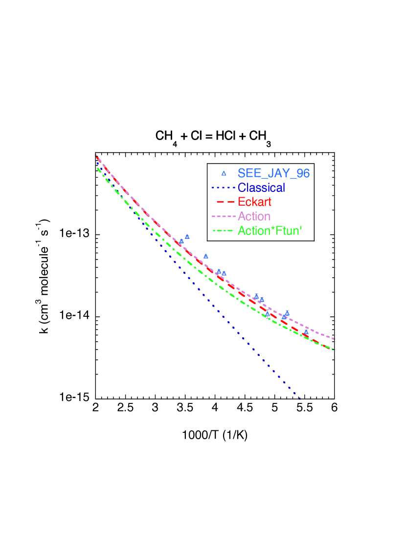
Figure 1: Plot of the temperature dependence of the thermal rate constants the $\rm Cl+CH_{4}\rightarrow HCl+CH_{3}$ reaction. The present results based on the evaluation of the tunneling probability for the quadratic expansion of the action are denoted with green dashed-dotted and purple dashed lines, for calculations with and without the EF included, respectively.

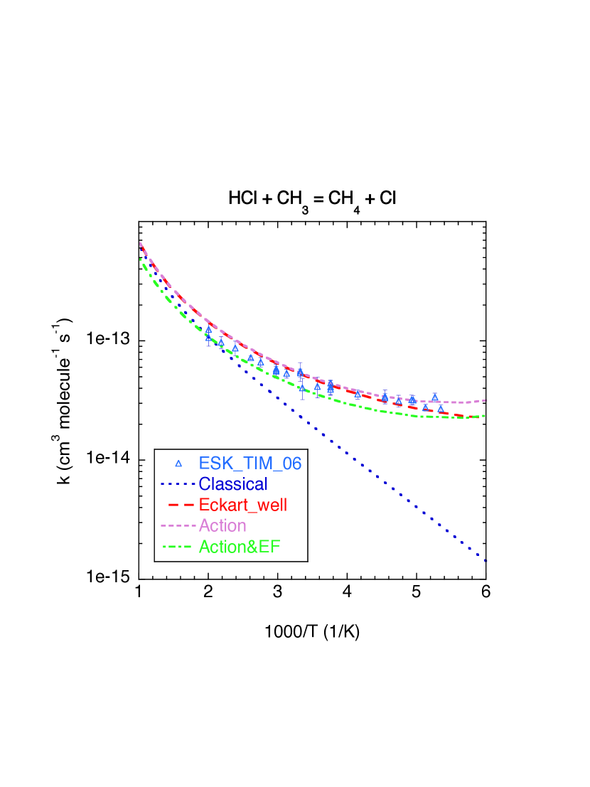
Figure 2: Plot of the temperature dependence of the thermal rate constants for the $\rm HCl+CH_{3}\rightarrow Cl+CH_{4}$ reaction. The present results based on the evaluation of the tunneling probability for the quadratic expansion of the action are denoted with green dashed-dotted and purple dashed lines, for calculations with and without the EF included, respectively.

The rate constants were calculated according to Eq. 1.5 employing CCSD(T)-F12/cc-pVQZ-F12 calculated rovibrational properties to evaluate $Z_{rot}^{\#}$ and $Z_{vib}^{\#}$ within the RRHO approximation. The tunneling factor $Z_{tun}^{\#}$ was evaluated via direct integration of Eq. 1.6 employing Eq. 5.9 to represent the tunneling probability. The action is evaluated with the quadratic expansion in energy. The integral in Eq. 1.6 is truncated at the bottom of the well.

The resulting predictions for the forward and reverse thermal rate constants are compared to the two lowest temperature experimental studies for the forward and reverse reactions in Figs. 1 and 2. For comparison purposes, we illustrate results with and without the EF, classical results (i.e., with $Z_{tun}^{\#}$ set to unity), and Eckart tunneling predictions. These Eckart predictions employ the zero-point corrected higher order energy estimates of the barrier relative to the van der Waals prereactive complexes, which yields a slightly lower $\alpha$ value of 1.4. Note though that the analytic expression for the Eckart tunneling factor is used here in place of the action expansion.

At the lowest temperatures tunneling is seen to increase the rate coefficient by about an order of magnitude. The present quadratic action based perturbative multi-dimensional tunneling approximation accurately captures this effect, with the experimental results generally falling between the results with and without the EF correction. The results for the reverse direction are in slightly better agreement with the experimental data, suggesting that there may be some minor inadequacy in the exothermicity/barrier calculation. Overall, the level of agreement is quite remarkable for a fully a priori calculation of the rate constants. The Eckart predictions are also in good agreement with the experimental data, which, as has been observed previously, is at least in part the result of some fortunate cancellation of errors.

5.6 Higher Order Expansion for One-Dimensional Problems

In some situations multi-dimensional effects are not important and the one-dimensional approximation provides a reasonable estimate of the value of $\alpha$ for a particular problem. We derive the corresponding expressions using a different method in Appendix F,

$$\alpha=\frac{\pi}{8}\left(\frac{5}{3}V_{3}^{2}-V_{4}\right),$$ (5.44)

where we have used a slightly different representation for the potential expansion, Eq. F.1. As it should be, $V_{3}$ always has a positive contribution to $\alpha$ and $V_{4}$ contributes with the opposite sign. From our derivation it is clear that $V_{3}$ and $V_{4}$ are the only terms in the one-dimensional potential expansion that contribute to $\alpha$. For reference purposes, we also provide the next tunneling action expansion coefficient $\alpha_{2}$, cf. Eq. 5.40, in terms of the potential anharmonicities, Eq. F.1, including the $120^{-1}V_{5}\omega_{b}^{7/2}q^{5}$ and $720^{-1}V_{6}\omega_{b}^{4}q^{6}$ terms,

$$\frac{\alpha_{2}}{\pi}=-\frac{1}{48}V_{6}+\frac{7}{48}V_{3}V_{5}+\frac{35}{384}V_{4}^{2}-\frac{35}{64}V_{3}^{2}V_{4}+\frac{385}{1152}V_{3}^{4},$$ (5.45)

which has been obtained from Eqs. F. and F.4.

It is interesting to find a potential, for which the action expansion in Eq. 5.10 is actually limited by the first two terms. In Appendix F it is shown that such a potential is given by the implicit equation,

$$q=y+\alpha\frac{\omega_{b}}{3\pi}y^{3},\ V(q)=\frac{1}{2}\omega_{b}^{2}y^{2}.$$ (5.46)

One can see that at small $y$, which correspond to small $q$, the potential is quadratic, $V(q)\propto q^{2}$, as it should be. At larger $y$, which correspond to larger $q$, the potential is flattened out and becomes proportional to $q^{2/3}$, $V(q)\propto q^{2/3}$.

5.7 Low Temperature Limitations

While for bimolecular reactions Eq. 1.6 is valid at all temperatures, for unimolecular decomposition at low temperatures it is not true. This can be seen already for the one-dimensional metastable potential, Fig. 3.

Figure 3: one-dimensional metastable potential

In Appendix G, it is shown that at very low temperatures, when the instanton trajectory is close to the bottom of the well, the abbreviated tunneling action is approximately equal to,

$$\tilde{S}(V^{\#}-E)=\tilde{S}^{\#}+\frac{E}{\omega_{0}}\ln\left(\frac{E}{eE_{0}}\right),\ \tilde{S}^{\#}=\tilde{S}(V^{\#}),$$ (5.47)

where $\omega_{0}$ is the harmonic frequency at the bottom of the well, $e$ is the natural logarithm base, and $E_{0}$ is the characteristics of the tunneling barrier, cf. Eq. G.4. In contrast with our previous consideration, the energy $E$ in Eq. 5.47 is counted from the bottom of the well upward. Substituting Eq. 5.47 into Eq. 5.9 or 1.10 and then integrating over $E$ according to Eq. 1.6, one obtains the expression for for $Z^{\#}_{tun}\simeq\exp(-\tilde{S}^{\#}+\beta V^{\#})$ at very low temperatures, $\beta\omega_{0}\gg 1$, which has an obviously wrong temperature dependence: The reactant partition function, to which only the ground state contributes, and the Boltzmann factor give together $\exp[-\beta(V^{\#}-\omega_{0}/2)]$ and so the rate constant at very low temperatures would read, $k\simeq(2\pi\beta)^{-1}\exp(-\tilde{S}^{\#}+\beta\omega_{0}/2)$, while the true rate constant, which corresponds mostly to the tunneling from the ground metastable state, should approach a constant. In contrast, as shown in Appendix G, Langer’s theory, for which the expression in the one-dimensional case formally corresponds to the SPA, Eq. 1.12, for the integral in Eq. 1.6, gives the correct result.

The mathematical reason for this behavior is that the SPA energy window in the integral in Eq. 1.6, cf. Eq. G.13 in Appendix G, goes far beyond the upper limit of integration and, therefore, the SPA is formally unapplicable. In Fig. 4 we show the ratio of the tunneling factor $Z^{\#}_{tun}$ obtained on the basis of Eq. 1.6 and in the SPA, Eq. 1.12, as a function of temperature for the cubic potential,

$$V(q)=\frac{1}{2}\omega_{0}^{2}q^{2}-\frac{1}{6}\sqrt{\frac{2}{3}}\omega_{0}^{5/2}D^{-1/2}q^{3},$$ (5.48)

where $D=V^{\#}/\omega_{0}$ is the barrier height in frequency units (for a cubic barrier $\omega_{b}=\omega_{0}$).

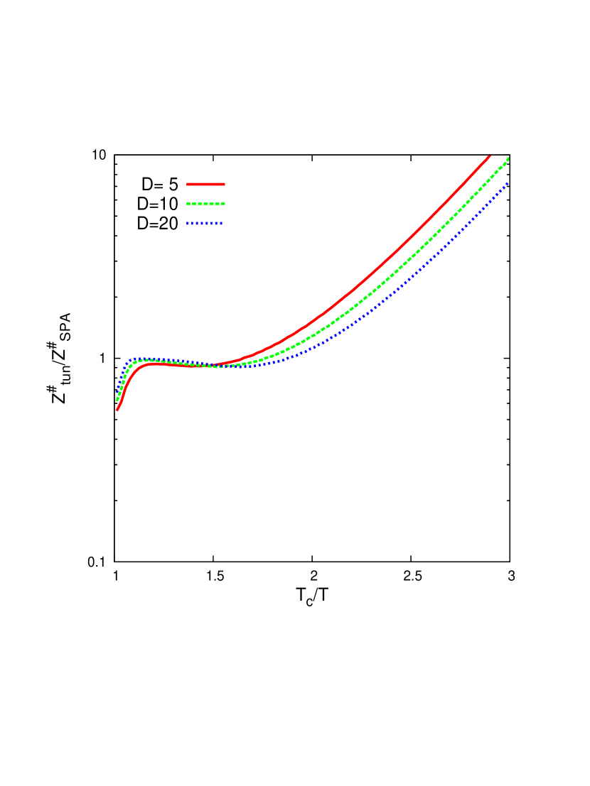
Figure 4: The ratio of the tunneling factor $Z^{\#}_{tun}$, Eq. 1.6, to its SPA approximation as a function of temperature for different values of the barrier height $D=V^{\#}/\omega_{0}$ for the cubic potential, Eq. 5.48

This ratio basically shows the error that one makes when one directly evaluates the integral over energy in Eq. 1.6 (for the one-dimensional or the multi-dimensional potential, does not matter) instead of using the SPA.

One may think that the expression with the integral over energy for the tunneling factor, Eq. 1.6, is more accurate than the SPA and that the SPA is just an approximation to it. The physical reason of inapplicability of Eq. 1.6 at very low temperatures is that it is based on the assumption that the dynamics in the well and the tunneling dynamics are independent processes. In the foundation of Eq. 1.6 lies the assumption that one can describe the tunneling effect in terms of the transmission coefficient for the incoming and outgoing semiclassical waves with an arbitrary energy. While at higer temperatures and, correspondingly, energies this is a reasonable assumption, for low temperatures this is not true at all. Only well-defined metastable states with certain energies do contribute to the rate constant. Therefore, to provide the expression analogous to Eq. 1.6 at low temperatures, one has to consider the tunneling from individual quantum states, which is a very difficult task in the multi-dimensional, non-separable case.

In contrast Langer’s theory does not consider tunneling with certain energies but rather considers the thermal process from the beginning. It is important to stress that the tunneling trajectory in Langer’s theory does not correspond to any real quantum state energy and is simply a mathematical construct. At relatively high energies when the density of states is sufficienty high, it corresponds to the energy region that gives the main contribution to the tunneling rate constant. At very low temperatures the energy of the tunneling trajectory is exponentially close to the bottom of the potential, see Eq. G.12 in Appendix G, and has nothing to do with the ground state energy.

5.8 Numerical Implementation

For practical numerical applications of Eqs. 3.11, 3.12, and 4.18 one must find the instanton trajectory as well as the stability parameters and the matrix $C_{\xi,\eta}$ for each considered energy.^{59, 60, 61} The instanton trajectory search is facilitated by the following considerations. One can start from the vicinity of the saddle point where the instanton trajectory is well known and corresponds to the motion along the unstable vibrational mode, the vectors $q_{i}$ and $p_{i}$ correspond to the transverse normal modes vectors with the appropriate normalization, and the stability parameters are $u_{i}=2\pi\omega_{i}/\omega_{b}$. For each subsequent energy, one can use the linearized equations of motion, Eq. 2.11, to obtain the monodromy transformation matrix $\hat{M}$ and then to obtain from it the new vectors $q_{i}$, $p_{i}$, and stability parameters $u_{i}$. To obtain $q_{E}$, which is the derivative of the instanton trajectory turning point with respect to the energy, one can use Eqs. 3.7, 3.8, and 4.2 and express the vector $q_{E}$ as a linear combination of the vectors $p_{i}$ and $g_{0}$. The “inertia moments matrix” $C_{\xi,\eta}$, Eq. 4.13, can be obtained by applying the monodromy transformation to the vectors $v^{J}_{\xi}$, Eq. 4.9, and considering the $q$-part of the resulting vectors. To make the next step by going down in energy, a new turning point can be used as a starting guess for the new trajectory. The new turning point is obtained by going along the vector $q_{E}$ and can be more accurately adjusted by shooting the trajectory and using the previous vectors $q_{i}$ and $p_{i}$ and the stability parameters for adjustment. It is interesting to note that in general $q_{E}$ does not coincide with (but is close to) $g_{0}$, which is the energy gradient in mass-weighted coordinates. Otherwise, the instanton trajectory turning point as a function of energy would coincide with the minimum energy path. This deviation is the manifestation of the coupling between the reaction coordinate and the transverse modes.

5.9 Anharmonicity in Low Frequency Modes

Sufficiently large chemical complexes usually have many modes including low-frequency ones. For such systems the second-order harmonic approximation, which is inherently present in Langer’s theory, may be too restrictive because for these modes considerable anharmonical corrections may be required even below the crossover temperature. To handle this situation one can use an ad hoc approach in which the full TS partition function is written in the following form,²⁶

$$Z^{\#}\simeq\frac{Z^{\#}_{AH}}{Z^{\#}_{RRHO}}Z^{\#}_{ins},$$ (5.49)

in which $Z^{\#}_{AH}$ is the anharmonic partition function for the TS with no tunneling, $Z^{\#}_{RRHO}$ is the partition function above the barrier in the harmonic approximation, Eq. 1.2, and $Z^{\#}_{ins}$ is the partition function with tunneling from Eq. 4.18. Equation 5.49 provides the correct expression for the partition function at high and low temperatures. If some anharmonic low frequency modes are not involved in the tunneling dynamics (i.e. they are uncoupled from the reaction coordinate) they naturally come into Eq. 5.49 as a factor and the corresponding harmonic terms are automatically cancelled out.

5.10 Correspondence between Negative Eigenvalues and Focal Points of the Instanton Trajectory

The instanton trajectory corresponds to a saddle point in the configurational space of closed paths. This feature means that there should be only one negative eigenvalue in the quadratic action $S^{\prime}[\delta q]$, Eq. 2.6, considered for small deviations from the instanton trajectory. On the other hand, the path integral considered as a function of the final time is inversely proportional to the square root of the certain determinant $|q_{1}q_{2}...q_{N}|$, cf. Eq. 2.12. When the tunneling trajectory passes through the focal point this determinant becomes zero and the path integral diverges, which means that one more eigenvalue in the quadratic action $S^{\prime}[\delta q]$ has passed through zero. The determinant after passing the focal point changes sign. Thus, the number of focal points of the tunneling trajectory corresponds to the number of negative eigenvalues in the quadratic action $S^{\prime}[\delta q]$ and should be equal 1.

In the derivation of the rate constant expressions we assumed that the turning points for the instanton trajectory, in which the system comes to complete rest, $\dot{q}_{0}=0$, exist. We would like to give an argument in support of this assumption. From classical mechanics it is known that the minimization of the classical action, cf. Eq. 2.5, can be equivalently reformulated in the form of Maupertuis’s principle.³⁰ Let us consider the curve that connects two hypersurfaces of constant energy on both sides of the barrier separating reactants and products and that it is parametrized so as to satisfy $E=\dot{q}^{2}/2+V(q)$ condition. Then the true classical trajectory corresponds to the minimum of the abbreviated action, $\tilde{S}[q]$,

$$\tilde{S}=\int\dot{q}dq=\int\dot{q}^{2}d\tau,\ E=\dot{q}^{2}/2+V(q).$$ (5.50)

It is obvious that such a trajectory always exists and the points where it touches the $E=V(q)$ hypersurfaces are the turning points. Returning to the regular description and considering the variations of the turning points for the half-trajectory one concludes that this trajectory corresponds to the extremum of the tunneling action, Eq. 2.3.

6. Concluding Remarks

The tunneling effects for general, non-separable systems have been considered within the framework of Langer’s theory. A closed form rate expression has been obtained, which differs from the commonly used one by an additional term related to the system non-separability. We have also obtained a general rate expression that takes into account angular momentum conservation. A simple model has been suggested to describe the tunneling effects in the vicinity of the crossover temperature, which is based on the local potential properties near the saddle point.

Appendices

Appendix A. Derivation of the Prefactor $U(t)$ for the Harmonic Path Integral

In this section we use the notations $S^{\prime}(q,t)=S^{\prime}(0,q,t)$, and $K(q,t)=K(q,0,t)$. Then for small time steps $\delta t$ the time dependence of the prefactor $U(t)$ for the harmonic path integral can be obtained from,

$$U(t+\delta t)=U(t)(2\pi\delta t)^{-N/2}\int d^{N}qe^{-S^{\prime}(q,t)}e^{-q^{2}/2\delta t},$$ (A.1)

where we have used the expression for $K(q,\delta t)$ at small $\delta t$,

$$K(q,\delta t)=(2\pi\delta t)^{-N/2}e^{-q^{2}/2\delta t}.$$ (A.2)

The action $S^{\prime}(q,t)$ can be written as $S^{\prime}(q,t)=q(t)\dot{q}(t)/2$. Because $q(t)$ satisfies linear equations of motion, $\dot{q}(t)$ is a linear function of $q$,

$$\dot{q}(t)=\hat{G}(t)q.$$ (A.3)

Substituting Eq. A.3 into Eq. A.1 and expanding the exponent $e^{-S^{\prime}(q,t)}$ up to first order in $q$ (higher order terms correspond to higher orders in $\delta t$), one obtains,

$$U(t+\delta t)=U(t)(1-\frac{1}{2}\delta t\sum_{i}G_{i,i}),$$ (A.4)

On the other hand, considering the determinant $D(t)=|q^{(1)}(t),q^{(2)}(t),...,q^{(N)}(t)|$ for $N$ trajectories, which start with some initial velocities and zero coordinates, one finds, that

$$\frac{dD}{dt} =|\dot{q}^{(1)},q^{(2)},...,q^{(N)}|+|q^{(1)},\dot{q}^{(2)},...,q^{(N)}|$$

$$+...+|q^{(1)},q^{(2)},...,\dot{q}^{(N)}|.$$

Considering the velocities $\dot{q}^{(i)}(t)$ in the basis of $q^{(i)}(t)$, $\dot{q}^{(i)}(t)=\tilde{G}_{j,i}(t)q^{(j)}(t)$, one finds that $\frac{dD}{dt}=D\sum_{i}\tilde{G}_{i,i}$. But $\hat{\tilde{G}}=\hat{Q}^{-1}\hat{G}\hat{Q}$, where $Q_{i,j}=q_{i}^{(j)}(t)$, and the trace does not depend on the basis. Therefore,

$$\frac{dD}{dt}=\sum_{i}G_{i,i}D.$$ (A.6)

Substituting Eq. A.6 into Eq. A.4 one obtains,

$$\frac{1}{U}\frac{dU}{dt}=-\frac{1}{2}\frac{1}{D}\frac{dD}{dt},$$ (A.7)

whose solution is $U(t)=CD^{-1/2}$. Choosing the constant $C$ to match the determinant $D$ at small times $t$, $D(t)\simeq|t\dot{q}^{(0)}(0),t\dot{q}^{(1)}(0),...,t\dot{q}^{(N)}(0)|$, and taking into account that $U(t)$ at small times is given by, $U(t)\simeq(2\pi t)^{-N/2}$, cf. Eq. A.2, one arrives at Eq. 2.12.

Appendix B. Perturbation Theory for $U(T)$

We will calculate the determinant ratio R, cf. Eq. 2.12

$$R=\frac{|q^{(1)}(T+\tau),q^{(2)}(T+\tau),...,q^{(N)}(T+\tau)|}{|p^{(1)}(\tau),p^{(2)}(\tau),...,p^{(N)}(\tau)|},$$ (B.1)

in the leading order of $\tau$, which happens to be two, and we will use the notation $p=\dot{q}$. First one notes that the monodromy matrix is left unchanged with the time-shift $\tau$ if one uses for the shifted matrix the basis,

$$\tilde{v}_{i}=\hat{K}(\tau,0)v_{i},$$ (B.2)

where $\hat{K}(t_{2},t_{1})$ is the time-propagator for the linearized equations of motion, Eq. 2.11. From the definition of the monodromy matrix it follows that

$$\hat{K}(T,0)v_{i}=\hat{M}_{i,j}v_{j}.$$ (B.3)

Multiplying Eq. B.3 by $\hat{K}(\tau,0)$ one arrives at

$$\hat{K}(T+\tau,\tau)\tilde{v}_{i}=\hat{M}_{i,j}\tilde{v}_{j},$$ (B.4)

where we have used the periodicity of the tunneling trajectory, $\hat{K}(T+\tau,T)=\hat{K}(\tau,0)$.

Let us calculate $\hat{K}(\tau,0)$ up to the second order in $\tau$. From Eq. 2.11 it follows, that $\ddot{p}=-\hat{k}p$, where

$$\hat{k}=\frac{\partial^{2}V}{\partial q^{2}}$$

and we have used the fact that $\dot{\hat{k}}=\frac{\partial^{3}V}{\partial q^{3}}\dot{q}_{0}=0$ at the turning point. Therefore, the time-shifted coordinates and momenta read up to second order,

$$q(\tau) \simeq q+\tau p-\frac{1}{2}\tau^{2}\hat{k}q,$$ (B.5)

$$p(\tau) \simeq p-\tau\hat{k}q-\frac{1}{2}\tau^{2}\hat{k}p,$$

or in matrix form,

$$\hat{K}(\tau,0)\simeq\hat{I}+\tau\left(\begin{array}[]{cc}0&I\\ -\hat{k}&0\end{array}\right)+\frac{1}{2}\tau^{2}\left(\begin{array}[]{cc}-\hat{k}&0\\ 0&-\hat{k}\end{array}\right).$$ (B.6)

We will also need $\hat{K}(\tau,0)^{-1}$, which is given by,

$$\hat{K}(\tau,0)^{-1}\simeq\hat{I}-\tau\left(\begin{array}[]{cc}0&I\\ -\hat{k}&0\end{array}\right)+\frac{1}{2}\tau^{2}\left(\begin{array}[]{cc}-\hat{k}&0\\ 0&-\hat{k}\end{array}\right),$$ (B.7)

where we have used the identity $(\hat{I}+\tau\hat{A}+\tau^{2}\hat{B})^{-1}\simeq\hat{I}-\tau\hat{A}-\tau^{2}\hat{B}+\tau^{2}\hat{A}^{2}$.

We will use the the monodromy matrix eigenspace representation. The following matrix converts the eigenvectors coefficients into the $(q,p)$ representation,

$$\hat{A}=\left(\begin{array}[]{cccc}q_{E}&0&q_{i}&q_{i}\\ 0&g_{0}&p_{i}&-p_{i}\end{array}\right).$$ (B.8)

The inverted matrix $\hat{A}^{-1}$ is given by

$$\hat{A}^{-1}=\left(\begin{array}[]{cc}g_{0}&0\\ 0&q_{E}\\ \frac{1}{2}p_{i}&\frac{1}{2}q_{i}\\ \frac{1}{2}p_{i}&-\frac{1}{2}q_{i}\end{array}\right).$$ (B.9)

The monodromy matrix in its eigenspace representation is given by,

$$\hat{M}=\left(\begin{array}[]{cccc}1&0&0&0\\ \frac{dT}{dE}&1&0&0\\ 0&0&\lambda_{i}&0\\ 0&0&0&\lambda_{i}^{-1}\end{array}\right).$$ (B.10)

Then, the conversion from the initial momenta to the final coordinates is given by the matrix $\hat{F}$,

$$\hat{F}=\hat{K}(\tau,0)\hat{A}\hat{M}\hat{A}^{-1}\hat{K}^{-1}(\tau,0),$$ (B.11)

whose expansion up to second order in $\tau$ is given by,

$$\hat{F}\simeq\hat{A}\hat{M}\hat{A}^{-1}$$ (B.12)

$$+\tau(\hat{K}_{1}\hat{A}\hat{M}\hat{A}^{-1}-\hat{A}\hat{M}\hat{A}^{-1}\hat{K}_{1})$$

$$+\frac{1}{2}\tau^{2}(\hat{K}_{1}^{2}A\hat{M}\hat{A}^{-1}+\hat{A}\hat{M}\hat{A}^{-1}\hat{K}_{1}^{2}-2\hat{K}_{1}\hat{A}\hat{M}\hat{A}^{-1}\hat{K}_{1})+...,$$

$$\hat{K}_{1}=\left(\begin{array}[]{cc}0&I\\ -\hat{k}&0\end{array}\right).$$ (B.15)

Now we turn to the calculation of the result of the application of $\hat{F}$ to individual vectors. First we consider the trajectory with initial momentum $g_{0}$. In zeroth order it is given by,

$$\hat{A}\hat{M}\hat{A}^{-1}\left(\begin{array}[]{c}0\\ g_{0}\end{array}\right)=\left(\begin{array}[]{c}0\\ g_{0}\end{array}\right),$$ (B.16)

which is the cause of the divergence of the determinant ratio at the focal point, Eq. B.1. The first order terms are given by,

$$\hat{K}_{1}\hat{A}\hat{M}\hat{A}^{-1}\left(\begin{array}[]{c}0\\ g_{0}\end{array}\right)=\hat{K}_{1}\left(\begin{array}[]{c}0\\ g_{0}\end{array}\right)=\left(\begin{array}[]{c}g_{0}\\ 0\end{array}\right),$$ (B.17)

$$\hat{A}\hat{M}\hat{A}^{-1}\hat{K}_{1}\left(\begin{array}[]{c}0\\ g_{0}\end{array}\right) = \hat{A}\hat{M}\hat{A}^{-1}\left(\begin{array}[]{c}g_{0}\\ 0\end{array}\right)$$ (B.22)

$$= g_{0}^{2}\left(\begin{array}[]{c}q_{E}\\ 0\end{array}\right)+\frac{dT}{dE}g_{0}^{2}\left(\begin{array}[]{c}0\\ g_{0}\end{array}\right)$$ (B.27)

$$+ \frac{1}{2}\sum_{i}p_{i}g_{0}\left[(\lambda_{i}+\lambda_{i}^{-1})\left(\begin{array}[]{c}q_{i}\\ 0\end{array}\right)+(\lambda_{i}-\lambda_{i}^{-1})\left(\begin{array}[]{c}0\\ p_{i}\end{array}\right)\right].$$ (B.32)

Collecting both terms, Eqs. B.17 and B.27, and taking into account that

$$g_{0}=g_{0}^{2}q_{E}+\sum_{i}(p_{i}g_{0})q_{i}$$ (B.33)

one obtains for the first order correction $q^{1st}_{0}$ to the $q$-vector of the trajectory with initial momentum $g_{0}$,

$$q^{1st}_{0}=\frac{\tau}{2}\sum_{i}p_{i}g_{0}(2-\lambda_{i}-\lambda_{i}^{-1})q_{i},$$ (B.34)

which does not contain any $q_{i}$-independent part. As a result, the correction to $R$, Eq. B.1, disappears in the first order over $\tau$.

We turn now to the calculation of the second order corrections to the $q$-vector with respect to $\tau$ for the trajectory with initial momentum $g_{0}$. Only terms with a $q$-part that is linearly independent of $q_{i}$ will contribute to the determinant in the numerator of Eq. B.1 to second order in $\tau$. Both terms,

$$\hat{K}_{1}^{2}\hat{A}\hat{M}\hat{A}^{-1}\left(\begin{array}[]{c}0\\ g_{0}\end{array}\right)=\left(\begin{array}[]{c}0\\ -\hat{k}g_{0}\end{array}\right)$$ (B.35)

and

$$\hat{A}\hat{M}\hat{A}^{-1}\hat{K}_{1}^{2}\left(\begin{array}[]{c}0\\ g_{0}\end{array}\right)=\hat{A}\hat{M}\hat{A}^{-1}\left(\begin{array}[]{c}0\\ -\hat{k}g_{0}\end{array}\right),$$ (B.36)

do not give a contribution to the $q$-part of the vector that is linearly independent of $q_{i}$. The cross-term is given by,

$$\hat{K}_{1}\hat{A}\hat{M}\hat{A}^{-1}\hat{K}_{1}\left(\begin{array}[]{c}0\\ g_{0}\end{array}\right)=\hat{K}_{1}\left\{g_{0}^{2}\left(\begin{array}[]{c}q_{E}\\ 0\end{array}\right)+\frac{dT}{dE}g_{0}^{2}\left(\begin{array}[]{c}0\\ g_{0}\end{array}\right)\right.$$ (B.43)

$$+\left.\frac{1}{2}\sum_{i}p_{i}g_{0}\left[(\lambda_{i}+\lambda_{i}^{-1})\left(\begin{array}[]{c}q_{i}\\ 0\end{array}\right)+(\lambda_{i}-\lambda_{i}^{-1})\left(\begin{array}[]{c}0\\ p_{i}\end{array}\right)\right]\right\}$$ (B.48)

$$=\frac{dT}{dE}g_{0}^{2}\left(\begin{array}[]{c}g_{0}\\ 0\end{array}\right)+\frac{1}{2}\sum_{i}p_{i}g_{0}(\lambda_{i}-\lambda_{i}^{-1})\left(\begin{array}[]{c}p_{i}\\ 0\end{array}\right)+...$$ (B.53)

where we did not include the momentum part of the final vector. Using the relation,

$$p_{i}=(p_{i}g_{0})q_{E}+\sum_{j}(p_{i}p_{j})q_{j},$$ (B.54)

and taking into account Eq. B.33, one obtains the second order correction $q^{2nd}_{0}$ to the $q$-vector of the trajectory with initial momentum $g_{0}$,

$$q^{2nd}_{0}=-\tau^{2}\left[\frac{dT}{dE}g_{0}^{2}+\frac{1}{2g_{0}^{2}}\sum_{i}(p_{i}g_{0})^{2}(\lambda_{i}-\lambda_{i}^{-1})\right]g_{0}+...$$ (B.55)

Next we turn to the calculation of the $q$-vectors for the trajectories with initial momenta $p_{i}$. Only the terms up to first order in $\tau$ will contribute and only $q_{i}$-independent parts of the first order terms should be considered. The zero-order term is given by

$$\hat{A}\hat{M}\hat{A}^{-1}\left(\begin{array}[]{c}0\\ p_{i}\end{array}\right)=\frac{1}{2}(\lambda_{i}+\lambda_{i}^{-1})\left(\begin{array}[]{c}0\\ p_{i}\end{array}\right)+\frac{1}{2}(\lambda_{i}-\lambda_{i}^{-1})\left(\begin{array}[]{c}q_{i}\\ 0\end{array}\right).$$ (B.56)

The first order terms are given by,

$$\hat{K}_{1}\hat{A}\hat{M}\hat{A}^{-1}\left(\begin{array}[]{c}0\\ p_{i}\end{array}\right) = \frac{1}{2}(\lambda_{i}+\lambda_{i}^{-1})\left(\begin{array}[]{c}p_{i}\\ 0\end{array}\right)+...$$ (B.61)

$$= \frac{1}{2}(\lambda_{i}+\lambda_{i}^{-1})\frac{p_{i}g_{0}}{g_{0}^{2}}\left(\begin{array}[]{c}g_{0}\\ 0\end{array}\right)+...$$ (B.64)

$$\hat{A}\hat{M}\hat{A}^{-1}\hat{K}_{1}\left(\begin{array}[]{c}0\\ p_{i}\end{array}\right) = \hat{A}\hat{M}\hat{A}^{-1}\left(\begin{array}[]{c}p_{i}\\ 0\end{array}\right)=\frac{p_{i}g_{0}}{g_{0}^{2}}\left(\begin{array}[]{c}g_{0}\\ 0\end{array}\right)+...,$$ (B.71)

where we have again used Eqs. B.33 and B.54. Collecting the terms given by Eqs. B.64 and B.71 one obtains that the first order correction $q^{1st}_{i}$ to the $q$-vector for the trajectory with initial momentum $p_{i}$ is given by,

$$q^{1st}_{i}=\frac{\tau}{2}(\lambda_{i}+\lambda_{i}^{-1}-2)\frac{p_{i}g_{0}}{g_{0}^{2}}g_{0}+...$$ (B.72)

Substituting Eqs. B.34, B.55, and B.72 into Eq. B.1, one obtains,

$$R\simeq-\tau^{2}\left[\frac{dT}{dE}g_{0}^{2}+\frac{2}{g_{0}^{2}}\sum_{i}(p_{i}g_{0})^{2}\frac{\lambda_{i}+\lambda_{i}^{-1}-2}{\lambda_{i}-\lambda_{i}^{-1}}\right]\frac{|g_{0},q_{i}|}{|g_{0},p_{i}|}\prod_{i}\frac{\lambda_{i}-\lambda_{i}^{-1}}{2}.$$ (B.73)

Appendix C. Perturbation Theory for $U(T)$ in the Angular Momentum Conservation Case

The derivation is completely analogous to the previous section. Equations B.2-B.7 and B.11 stay as they are. Equations B.8-B.10 are modified as follows,

$$\hat{A}=\left(\begin{array}[]{cccccc}q_{E}&0&q_{\xi}&0&q_{i}&q_{i}\\ 0&g_{0}&0&p_{\xi}&p_{i}&-p_{i}\end{array}\right).$$ (C.1)

The inverted matrix $\hat{A}^{-1}$ is given by

$$\hat{A}^{-1}=\left(\begin{array}[]{cc}g_{0}&0\\ 0&q_{E}\\ p_{\xi}&0\\ 0&q_{\xi}\\ \frac{1}{2}p_{i}&\frac{1}{2}q_{i}\\ \frac{1}{2}p_{i}&-\frac{1}{2}q_{i}\end{array}\right).$$ (C.2)

The monodromy matrix in its eigenspace representation is given by,

$$\hat{M}=\left(\begin{array}[]{cccccc}1&0&0&0&0&0\\ \frac{dT}{dE}&1&0&0&0&0\\ 0&0&\hat{I}&\hat{C}&0&0\\ 0&0&0&\hat{I}&0&0\\ 0&0&0&0&\hat{\lambda}&0\\ 0&0&0&0&0&\hat{\lambda}^{-1}\end{array}\right),$$ (C.3)

Relations B.33 and B.54 are substituted by,

$$g_{0} = g_{0}^{2}q_{E}+\sum_{i}(p_{i}g_{0})q_{i}+\sum_{\xi}(p_{\xi}g_{0})q_{\xi},$$ (C.4)

$$p_{i} = (p_{i}g_{0})q_{E}+\sum_{j}(p_{i}p_{j})q_{j}+\sum_{\xi}(p_{i}p_{\xi})q_{\xi},$$ (C.5)

$$p_{\xi} = (p_{\xi}g_{0})q_{E}+\sum_{j}(p_{\xi}p_{j})q_{j}+\sum_{\eta}(p_{\xi}p_{\eta})q_{\eta}.$$ (C.6)

Let us consider the trajectory with initial momentum $g_{0}$. For this trajectory Eqs. B.16-B.17 hold. The term $\hat{A}\hat{M}\hat{A}^{-1}\hat{K}_{1}$ is given by,

$$\hat{A}\hat{M}\hat{A}^{-1}\hat{K}_{1}\left(\begin{array}[]{c}0\\ g_{0}\end{array}\right)=\hat{A}\hat{M}\hat{A}^{-1}\left(\begin{array}[]{c}g_{0}\\ 0\end{array}\right)$$ (C.11)

$$=g_{0}^{2}\left(\begin{array}[]{c}q_{E}\\ 0\end{array}\right)+\frac{dT}{dE}g_{0}^{2}\left(\begin{array}[]{c}0\\ g_{0}\end{array}\right)+\sum_{\xi}(p_{\xi}g_{0})\left(\begin{array}[]{c}q_{\xi}\\ 0\end{array}\right)$$ (C.23)

$$+\frac{1}{2}\sum_{i}p_{i}g_{0}\left[(\lambda_{i}+\lambda_{i}^{-1})\left(\begin{array}[]{c}q_{i}\\ 0\end{array}\right)+(\lambda_{i}-\lambda_{i}^{-1})\left(\begin{array}[]{c}0\\ p_{i}\end{array}\right)\right],$$

Substituting Eq. C.4 into Eq. B.17 one can see that Eq. B.34 holds.

The $q$-part of the second order terms for the trajectory with initial momentum $g_{0}$ should be linearly independent of $q_{i}$ and $q_{\xi}$ because the linearly dependent terms have higher order dependence on $\tau$. Therefore, the terms $\hat{A}\hat{M}\hat{A}^{-1}\hat{K}^{2}_{1}$ and $\hat{K}^{2}_{1}\hat{A}\hat{M}\hat{A}^{-1}$ again give no independent contribution to the $q$-part of the trajectory with initial momentum $g_{0}$. For the cross-term $\hat{K}_{1}\hat{A}\hat{M}\hat{A}^{-1}\hat{K}_{1}$ Eq. B.53 stays and so does the second order correction $q^{2nd}_{0}$ expression, Eq. B.55.

For the trajectories with initial momenta $p_{i}$ and $p_{\xi}$ only the first order terms contribute to the second order term in Eq. B.1. Also, only the $q$-parts that are linearly independent of $q_{i}$ and $q_{\xi}$ will contribute to Eq. B.1 to the second order on $\tau$. For the trajectories with initial momenta $p_{i}$ Eqs. B.56-B.71 remain the same and so does the expression for the first order correction $q^{1st}_{i}$, Eq. B.72.

For the trajectories with initial momenta $p_{\xi}$, the zero order term $\hat{A}\hat{M}\hat{A}^{-1}$ is given by

$$\hat{A}\hat{M}\hat{A}^{-1}\left(\begin{array}[]{c}0\\ p_{\xi}\end{array}\right)=\sum_{\eta}C_{\xi,\eta}\left(\begin{array}[]{c}q_{\eta}\\ 0\end{array}\right)+\left(\begin{array}[]{c}0\\ p_{\xi}\end{array}\right).$$ (C.24)

The first order terms are given by,

$$\hat{K}_{1}\hat{A}\hat{M}\hat{A}^{-1}\left(\begin{array}[]{c}0\\ p_{\xi}\end{array}\right) = \left(\begin{array}[]{c}p_{\xi}\\ 0\end{array}\right)+...=\frac{p_{\xi}g_{0}}{g_{0}^{2}}\left(\begin{array}[]{c}g_{0}\\ 0\end{array}\right)+...$$ (C.31)

$$\hat{A}\hat{M}\hat{A}^{-1}\hat{K}_{1}\left(\begin{array}[]{c}0\\ p_{\xi}\end{array}\right) = \hat{A}\hat{M}\hat{A}^{-1}\left(\begin{array}[]{c}p_{\xi}\\ 0\end{array}\right)=\frac{p_{\xi}g_{0}}{g_{0}^{2}}\left(\begin{array}[]{c}g_{0}\\ 0\end{array}\right)+...,$$ (C.38)

and one can see that they cancel each other. Thus, there is no first order contribution to the $q$-vector from the trajectories with initial momenta $p_{\xi}$.

Collecting all the terms in Eq. B.1 together, one obtains,

$$R \simeq -\tau^{2}\left[\frac{dT}{dE}g_{0}^{2}+\frac{2}{g_{0}^{2}}\sum_{i}(p_{i}g_{0})^{2}\frac{\lambda_{i}+\lambda_{i}^{-1}-2}{\lambda_{i}-\lambda_{i}^{-1}}\right]$$

$$\times \frac{|g_{0},q_{i},\sum_{\eta}C_{\xi,\eta}q_{\eta}|}{|g_{0},q_{i},p_{\xi}|}\prod_{i}\frac{\lambda_{i}-\lambda_{i}^{-1}}{2}.$$

Appendix D. Entanglement Factor at Small Energies

The potential is described by Eq. 5.3 and only the cubic anharmonicity is considered. We start the trajectory from the turning point with small energy $E$. In the zeroth order approximation the trajectory is given by,

$$q^{0th}_{0}(t) = -q_{0}\cos(\omega_{b}t)=-\frac{1}{2}q_{0}e^{i\omega_{b}t}+c.c.,\ \frac{1}{2}\omega_{b}^{2}q_{0}^{2}=E,$$ (D.1)

$$q^{0th}_{i}(t) = 0.$$

The first order correction $q^{1st}_{i}(t)$ satisfies the following equations,

$$\ddot{q}_{0}^{1st}+\omega_{b}^{2}q^{1st}_{0} = -\frac{1}{2}V_{0,0,0}^{(3)}q_{0}^{0th^{2}},$$ (D.2)

$$\ddot{q}_{i}^{1st}-\omega_{i}^{2}q^{1st}_{i} = -\frac{1}{2}V_{0,0,i}^{(3)}q_{0}^{0th^{2}},$$ (D.3)

The solution of Eqs. D.2-D.3 is given by,

$$q^{1st}_{0}(t) = -\frac{1}{4}\frac{q_{0}^{2}}{\omega_{b}^{2}}V_{0,0,0}^{(3)}(1-\frac{1}{3}\cos(2\omega_{b}t)),$$ (D.4)

$$q^{1st}_{i}(t) = \frac{1}{4}q_{0}^{2}V_{0,0,i}^{(3)}(\omega_{i}^{-2}+\frac{1}{4\omega_{b}^{2}+\omega_{i}^{2}}\cos(2\omega_{b}t)).$$ (D.5)

Then the potential gradient $g_{0}=\partial V/\partial q$ at the turning point is given by,

$$\frac{\partial V}{\partial q_{0}} \simeq -\omega_{b}^{2}q_{0},$$ (D.6)

$$\frac{\partial{V}}{\partial{q}_{i}} \simeq -\omega_{i}^{2}q_{i}^{1st}(0)+\frac{1}{2}V^{(3)}_{i,0,0}q_{0}^{0th}(0)^{2}=q_{0}^{2}V_{0,0,i}^{(3)}\frac{\omega_{b}^{2}}{4\omega_{b}^{2}+\omega_{i}^{2}}.$$ (D.7)

We proceed with calculating the eigenvectors $v_{i,\pm}=(q_{i},\pm p_{i})$ of the monodromy transformaiton. To obtain the monodromy matrix one can use Eqs. 2.11. To zeroth order the solutions of these equations, which correspond to the eigenvectors $v_{i,\pm}$, are given by,

$$q^{0th}_{i,\pm,j}(t)=\delta_{i,j}q_{i}^{0}e^{\pm\omega_{i}t},$$ (D.8)

$$q_{i}^{0}=\omega_{i}^{-1/2},$$ (D.9)

where Eq. D.9 is the consequence of the orthogonality relation, Eq. 3.3. To first order with respect to the potential anharmonicity one can neglect the change in the instanton trajectory. Then the first order correction to $q^{0th}_{i,+,j}(t)$ satisfies the following equations (the correction to $q^{0th}_{i,-,j}(t)$ is obtained by changing the sign in the exponent, so we omit the $\pm$ index in the notation),

$$\ddot{q}^{1st}_{i,0}+\omega_{b}^{2}q^{1st}_{i,0}=-V^{(3)}_{0,0,i}q_{0}^{0th}q_{i}^{0}e^{\omega_{i}t},$$ (D.10)

$$\ddot{q}^{1st}_{i,j}-\omega_{j}^{2}q^{1st}_{i,j}=-V^{(3)}_{0,i,j}q_{0}^{0th}q_{i}^{0}e^{\omega_{i}t},$$ (D.11)

where $q_{0}^{0th}$ is given by Eq. D.1. The solution of Eqs. D.10-D.11 is given by,

$$q^{1st}_{i,0}(t)=\frac{1}{2}V^{(3)}_{0,0,i}q_{0}q_{i}^{0}\left(\frac{e^{(i\omega_{b}+\omega_{i})t}}{(i\omega_{b}+\omega_{i})^{2}+\omega_{b}^{2}}+c.c.\right),$$ (D.12)

$$q^{1st}_{i,j}(t)=\frac{1}{2}V^{(3)}_{0,i,j}q_{0}q_{i}^{0}\left(\frac{e^{(i\omega_{b}+\omega_{i})t}}{(i\omega_{b}+\omega_{i})^{2}-\omega_{j}^{2}}+c.c.\right),$$ (D.13)

From Eqs. D.12-D.13 one can see that in the first order approximation, the stability parameters $u_{i}=2\pi\omega_{i}/\omega_{b}$ do not change and that $(q_{i}^{1st},\dot{q}_{i}^{1st})$ provide the first order corrections to the corresponding eigenvectors. We focus on Eq. D.12, which corresponds to the projection of the eigenvector on the reaction coordinate, as only it contributes to leading order. The first order correction to the momentum $p_{i}$ is given by $\dot{q}_{i,0}^{1st}$,

$$\dot{q}_{i,0}^{1st} = \frac{1}{2}V^{(3)}_{0,0,i}q_{0}q_{i}^{0}\left(\frac{i\omega_{b}+\omega_{i}}{\omega_{i}(i2\omega_{b}+\omega_{i})}+c.c.\right)$$ (D.14)

$$= \frac{1}{2}V^{(3)}_{0,0,i}q_{0}q_{i}^{0}\left(\frac{1}{\omega_{i}}+\frac{\omega_{i}}{\omega_{i}^{2}+4\omega_{b}^{2}}\right).$$

The correction to the momentum changes sign when one considers the conjugated eigenvector $v_{i,-}$, which corresponds to the decaying exponent in Eq. D.8 and negative sign for $\omega_{i}$ in Eq. D.14, as it should be. Using Eqs. D.6, D.7, and D.14, one obtains that $p_{i}g_{0}$ to leading order with respect to energy is given by,

$$p_{i}g_{0}=-2V^{(3)}_{0,0,i}q_{0}^{2}q_{i}^{0}\omega_{b}^{4}\omega_{i}^{-1}(\omega_{i}^{2}+4\omega_{b}^{2})^{-1}.$$ (D.15)

Substituting Eq. D.15 into Eq. 5.1 and using Eqs. D.6 and D.9, one obtains Eq. 5.2 approaches as the temperature approaches the crossover.

Appendix E. Action Anharmonicity $\alpha$ for Multi-Dimensional Potential

To calculate $\alpha$ we use the relation $\alpha=\frac{1}{2}\omega_{b}^{2}\frac{dT}{dE}|_{E=0}$. We start the trajectory from the saddle point with small energy $E$ and then calculate the anharmonic correction to the period of the harmonic oscillator $T_{0}=2\pi/\omega_{b}$ with second order perturbation theory. In the zeroth order approximation the trajectory is given by,

$$q^{0th}_{0}(t) = q_{0}\sin(\omega_{b}t),\ \frac{1}{2}\omega_{b}^{2}q_{0}^{2}=E,$$ (E.1)

$$q^{0th}_{i}(t) = 0.$$

The first order correction $q^{1st}_{i}(t)$ satisfies the following equations,

$$\ddot{q}_{0}^{1st}+\omega_{b}^{2}q^{1st}_{0} = -\frac{1}{2}V_{0,0,0}^{(3)}q_{0}^{0th^{2}},$$ (E.2)

$$\ddot{q}_{i}^{1st}-\omega_{i}^{2}q^{1st}_{i} = -\frac{1}{2}V_{0,0,i}^{(3)}q_{0}^{0th^{2}},$$ (E.3)

The solution of Eqs. E.2-E.3 is given by,

$$q^{1st}_{0}(t) = -\frac{1}{4}\frac{q_{0}^{2}}{\omega_{b}^{2}}V_{0,0,0}^{(3)}(1+\frac{1}{3}\cos(2\omega_{b}t)),$$ (E.4)

$$q^{1st}_{i}(t) = \frac{1}{4}q_{0}^{2}V_{0,0,i}^{(3)}(\omega_{i}^{-2}-\frac{1}{4\omega_{b}^{2}+\omega_{i}^{2}}\cos(2\omega_{b}t)).$$ (E.5)

It is worth noting that, while the first order corrections, Eqs. E.4-E.5, modify the trajectory energy slightly, this change is of the order of $~{}E^{2}$ or higher and, therefore, can be neglected. From Eq. E.4 one can see that the period does not change in the first order of perturbation theory. The equation for the second order correction to the reaction coordinate $q_{0}^{2nd}$ reads,

$$\ddot{q}_{0}^{2nd}+\omega_{b}^{2}q^{2nd}_{0}=-V_{0,0,0}^{(3)}q_{0}^{0th}q_{0}^{1st}-\sum_{i}V_{0,0,i}^{(3)}q_{0}^{0th}q_{i}^{1st},$$ (E.6)

whose solution is given by (we keep only the terms that change over the period),

$$q_{0}^{2nd}(t)=-t\cos(\omega_{b}t)\frac{1}{8}\left[\frac{5}{6}V_{0,0,0}^{(3)^{2}}\frac{q_{0}^{3}}{\omega_{b}^{3}}-\sum_{i}V_{0,0,i}^{(3)^{2}}\frac{q_{0}^{3}}{\omega_{b}}\left(\omega_{i}^{-2}+\frac{1}{2}\frac{1}{4\omega_{b}^{2}+\omega_{i}^{2}}\right)\right]+...$$ (E.7)

Thus, the change in the reaction coordinate $\delta q_{0}$ during the full period $2\pi/\omega_{b}$ is given by,

$$\delta q_{0}=-\frac{\pi}{4}\left[\frac{5}{6}V_{0,0,0}^{(3)^{2}}\frac{q_{0}^{3}}{\omega_{b}^{4}}-\sum_{i}V_{0,0,i}^{(3)^{2}}\frac{q_{0}^{3}}{\omega_{b}^{2}}\left(\omega_{i}^{-2}+\frac{1}{2}\frac{1}{4\omega_{b}^{2}+\omega_{i}^{2}}\right)\right].$$ (E.8)

The corresponding change in the period $\delta T=-\delta q_{0}/\dot{q}_{0}^{0th}=-\delta q_{0}/(q_{0}\omega_{b})$ and $\alpha$ is given by Eq. 5.27. For the potential with fourth order anharmonicities, $\alpha$ is obtained in the first order approximation in a similar fashion and is given by Eq. 5.28.

We proceed with the derivation of the multi-dimensional correction to $\alpha$ in the MEP approximation, in which the tunneling path follows the potential gradient. In the vicinity of the saddle point the deviation from the $q_{0}$ direction happens mainly due to the $V^{(3)}_{0,0,i}$ term in the potential and the MEP satisfies the following equation,

$$\frac{dq_{i}}{dq_{0}}=\frac{1}{2}\frac{V^{(3)}_{0,0,i}}{\omega_{b}^{2}}q_{0}-\frac{\omega_{i}^{2}}{\omega_{b}^{2}}\frac{q_{i}}{q_{0}},$$ (E.9)

whose solution is given by,

$$q_{i} = \frac{1}{2}\frac{V^{(3)}_{0,0,i}}{2\omega_{b}^{2}+\omega_{i}^{2}}q_{0}^{2},$$ (E.10)

$$\frac{dq_{i}}{dq_{0}} = \frac{V^{(3)}_{0,0,i}}{2\omega_{b}^{2}+\omega_{i}^{2}}q_{0}.$$ (E.11)

Then the abbreviated action, which is given by Eq. 2.20, can be written as,

$$\tilde{S}(E) = \oint{d}q_{0}\sqrt{2E-\omega_{b}^{2}q_{0}^{2}+\sum_{i=1}(\omega_{i}^{2}q_{i}^{2}-V^{(3)}_{0,0,i}q_{0}^{2}q_{i})-...}\sqrt{1+\sum_{i=1}(dq_{i}/dq_{0})^{2}}$$ (E.12)

$$= \frac{1}{8}\sum_{i=1}\frac{V^{(3)^{2}}_{0,0,i}}{(2\omega_{b}^{2}+\omega_{i}^{2})^{2}}\oint{d}q_{0}\left(4q_{0}^{2}\sqrt{2E-\omega_{b}^{2}q_{0}^{2}}-q_{0}^{4}\frac{4\omega_{b}^{2}+\omega_{i}^{2}}{\sqrt{2E-\omega_{b}^{2}q_{0}^{2}}}\right)+...$$

$$= -\frac{1}{8}\sum_{i=1}\frac{V^{(3)^{2}}_{0,0,i}}{\omega_{b}^{2}}\frac{8\omega_{b}^{2}+3\omega_{i}^{2}}{(2\omega_{b}^{2}+\omega_{i}^{2})^{2}}\oint{d}q_{0}q_{0}^{2}\sqrt{2E-\omega_{b}^{2}q_{0}^{2}}+...$$

$$= -\frac{\pi}{8}E^{2}\sum_{i=1}\frac{V^{(3)^{2}}_{0,0,i}}{\omega_{b}^{5}}\frac{8\omega_{b}^{2}+3\omega_{i}^{2}}{(2\omega_{b}^{2}+\omega_{i}^{2})^{2}}+...,$$

where we did not include one-dimensional and small terms. Then the multi-dimensional correction to $\alpha$ in the MEP approximation is given by Eq. 5.29.

Appendix F. The Relation between the One-Dimensional Potential and Abbreviated Action Expansions

In this section we assume that the potential is written in the following form,

$$V(q)=\frac{1}{2}\omega_{b}^{2}q^{2}+\frac{1}{6}V_{3}\omega_{b}^{5/2}q^{3}+\frac{1}{24}V_{4}\omega_{b}^{3}q^{4}+....$$ (F.1)

In mass-weighted coordinates $q$ has the dimensionality of $[E]^{-1/2}$ and therefore the third and fourth order anharmonicity parameters $V_{3}$ and $V_{4}$ are dimension-less.

The abbreviated action $\tilde{S}(E)$ corresponding to the potential $V(q)$ can be written as,

$$\tilde{S}(E)=\oint dq\sqrt{2(E-V(q))},$$ (F.2)

and the integral in Eq. F.2 is considered in the complex plane along a contour that is assumed to be large enough to surround the turning points. Then Eq. F.2 can be expanded as,

$$\tilde{S}(E) = i\sqrt{2}\oint dq\sqrt{V(q)}\sqrt{1-E/V(q)}$$

$$= i\sqrt{2}\oint dq(\sqrt{V(q)}-\frac{1}{2}EV(q)^{-1/2}-\frac{1}{8}E^{2}V^{-3/2}+...).$$

Each sequential term corresponds to the next order in the expansion of $\tilde{S}(E)$ over $E$. For the zero-order term one, of course, gets zero contribution because the $\sqrt{V(q)}$ expansion contains only positive powers of $q$. Representing $\sqrt{V(q)}$ in the form,

$$\sqrt{V(q)} = 2^{-1/2}\omega_{b}qF(q)^{1/2},$$ (F.4)

$$F(q) = 1+\frac{1}{3}V_{3}\sqrt{\omega_{b}}q+\frac{1}{12}V_{4}\omega_{b}q^{2}+...,$$

one can see that to calculate the $n$-th order term one needs to find the coefficient in front of $q^{2n-2}$ in the expansion of $F(q)^{-(2n-1)/2}$. Then the first order term is $\frac{2\pi E}{\omega_{b}}$ ($\oint dq/q=2\pi i$) and the second order term is $\pi(\frac{5}{24}V_{3}^{2}-\frac{1}{8}V_{4})E^{2}/\omega_{b}^{2}$. Comparing with Eq. 5.10, one arrives at Eq. 5.44.

In the following we find a potential for which the action expansion in Eq. 5.10 is limited to the first two terms. To this end we transform Eq. F.2 a bit differently, namely we introduce another variable $y=\sqrt{V(q)}$ and use it as an independent one. Because $V(q)$ is an analytic function of $q$, whose expansion starts with a quadratic term, $q$ is also an analytic function of $y$ whose expansion starts with a linear term. The expression for $\tilde{S}$ then reads,

$$\tilde{S}(E)=\sqrt{2}\oint dy\sqrt{E-y^{2}}\frac{dq}{dy},$$ (F.5)

Expanding $dq/dy=\sum_{n=0}^{\infty}A_{n}y^{n}$, one obtains,

$$\tilde{S}(E)=\sqrt{2}\sum_{i=0}^{\infty}A_{n}\oint dy\sqrt{E-y^{2}}y^{n},$$ (F.6)

Then we substitute $t=\sqrt{E}/y$ and take powers of $E$ out of the integrals getting as a result,

$$\tilde{S}(E)=i\sqrt{2}\sum_{i=0}^{\infty}A_{n}E^{n/2+1}\oint dt\sqrt{1-t^{2}}t^{-n-3},$$ (F.7)

Note that the integration contour now surrounds $t=0$ but not the turning points. Expanding the function $\sqrt{1-t^{2}}$ one notes that only even terms contribute to $\tilde{S}(E)$. We will assume that $A_{2n+1}=0$. Then for the first two terms one obtains,

$$\tilde{S}(E)=\sqrt{2}\pi A_{0}E+2^{-3/2}\pi A_{2}E^{2}.$$ (F.8)

Comparing with Eq. 5.10 one finds that $A_{0}=\sqrt{2}/\omega_{b}$ and $A_{2}=2^{3/2}\pi^{-1}\alpha/\omega_{b}^{2}$. All other $A_{n}=0$. Now remembering that $A_{n}$ are expansion coefficients of $dq/dy$ over powers of $y$, one obtains the following equation,

$$\frac{dq}{dy}=A_{0}+A_{2}y^{2},$$ (F.9)

whose solution is

$$q=A_{0}y+\frac{A_{2}}{3}y^{3},$$ (F.10)

where we have taken into account that $y=0$ at $q=0$. Substituting the expressions for $A_{0}$ and $A_{2}$ and remembering that $y=\sqrt{V(q)}$, one obtains the implicit equation for $V(q)$, Eq. 5.46.

Appendix G. Tunneling Rate Constant at Low Temperatures for One-Dimensional Metastable Potential

In this appendix we show that Langer’s theory gives the correct rate constant at very low temperatures, $\beta\omega_{0}\gg 1$. We calculate the tunneling period $T(V^{\#}-E)$ and the abbreviated action $\tilde{S}(V^{\#}-E)$ for the potential shown in Fig. 3 (we use now the real potential, not the inverted one) at the energy $E$ close to the bottom of the well, which is now counted from the bottom of the real well upward. We will assume that in the vicinity of the potential minimum the potental energy is exactly quadratic,

$$V(q)=\frac{1}{2}\omega_{0}^{2}q^{2},\ q<q_{2},$$ (G.1)

where $\omega_{0}$ is the frequency at the bottom of the well. This assumption, while it does not affect the final result, simplifies the derivation. Then, the tunneling period at energy $E$ counted from the bottom of the well can be written as,

$$T(V^{\#}-E)=2\left(\int_{q_{-}}^{q_{2}}\frac{dq}{\sqrt{\omega_{0}^{2}q^{2}-2E}}+\int_{q_{2}}^{q_{+}}\frac{dq}{\sqrt{2(V(q)-E)}}\right),$$ (G.2)

where $q_{\pm}$ are the turning points, see Fig. 3. Considering the expansion of the period $T$ over energy $E$ at small $E$ one finds that the second term gives some constant and higher order terms $E^{n},\ n>0$, while the first term gives $2\ln(2q_{2}/q_{-})/\omega_{0}$, where we have used the identity

$$\int\frac{dq}{\sqrt{q^{2}-a^{2}}}=\ln\!\left[q/a+\sqrt{(q/a)^{2}-1}\right].$$ (G.3)

Collecting the two terms and taking into account that $q_{-}=\sqrt{2E}/\omega_{0}$ one obtains,

$$T(V^{\#}-E)=-\frac{1}{\omega_{0}}\ln(E/E_{0})+...,$$ (G.4)

where the constant $E_{0}$ corresponds to the zero-order term in the expansion of $T$ over $E$ and higher order terms are not considered. Integrating Eq. G.4, one arrives at Eq. 5.47.

The tunneling rate constant at very low temperatures, $\beta\omega_{0}\gg 1$, corresponds to the decay of the ground state. The tunneling rate constant for the metastable ground state wave function $\psi(q)$ can be written as a probability flux $j$ to the right of the barrier,⁶²

$$k=\frac{i}{2}\left(\psi\frac{d\psi^{*}}{dq}-\psi^{*}\frac{d\psi}{dq}\right).$$ (G.5)

Far to the right of the turning point $q_{+}$ the semiclassical approximation is applicable and is given by,⁶²

$$\psi(q)\simeq C_{+}p^{-1/2}e^{i\int_{q_{+}}^{q}dq^{\prime}p(q^{\prime})},$$ (G.6)

$$p(q)=\sqrt{2(E-V(q))},\ q>q_{+}.$$

Substituting Eq. G.6 into Eq. G.5 one obtains that $k=|C_{+}|^{2}$.

To calculate the normalization constant $C_{+}$ one needs to trace the wave function $\psi(q)$ all the way to the well. According to the correspondence rule the wave function to the left of the barrier is given by⁶²

$$\psi(q)\simeq C_{+}p^{-1/2}e^{\int^{q_{+}}_{q}dq^{\prime}p(q^{\prime})},$$ (G.7)

$$p(q)=\sqrt{2(V(q)-E)},\ q<q_{+},$$

where only the growing to the left exponent is considered. Tracing it all the way to the left one can write an expression for $\psi(q)$ in the vicinity of the left turning point $q_{-}$, to the right of it,

$$\psi(q)\simeq C_{+}e^{\frac{1}{2}\tilde{S}(V^{\#}-E)}p^{-1/2}e^{-\int_{q_{-}}^{q}dq^{\prime}p(q^{\prime})},$$ (G.8)

$$p(q)=\sqrt{2(V(q)-E)},\ q_{-}<q,$$

Assuming that $E=\omega_{0}/2$ (the ground state) and using Eq. G.1 one can expand the power of the exponent in $\exp(-\int_{q_{-}}^{q}dq^{\prime}p(q^{\prime}))$ as,

$$\int_{q_{-}}^{q}dq^{\prime}p(q^{\prime})=\omega_{0}\int_{q_{-}}^{q}dq^{\prime}\sqrt{q^{\prime 2}-\omega_{0}^{-1}}$$ (G.9)

$$\simeq\frac{1}{2}(\omega_{0}q^{2}-\ln(2e^{1/2}\omega_{0}^{1/2}q)),\ q_{-}=\omega_{0}^{-1/2},$$

where we have used the identity,

$$\int dq\sqrt{q^{2}-a^{2}}=\frac{1}{2}\left(q\sqrt{q^{2}-a^{2}}-a^{2}\ln\!\left[q/a+\sqrt{(q/a)^{2}-1}\right]\right).$$ (G.10)

Substituting Eq. G.9 into Eq. G.8 and comparing the result with the ground wave function of the harmonic oscillator,⁶² $\psi(q)=(\omega_{0}/\pi)^{1/4}\exp(-\omega_{0}q^{2}/2)$, one obtains that,

$$k=\frac{\omega_{0}}{2\pi^{1/2}e^{1/2}}e^{-\tilde{S}(V^{\#}-\omega_{0}/2)}=\frac{1}{\sqrt{2\pi}}\sqrt{\omega_{0}E_{0}}e^{-\tilde{S}^{\#}}$$ (G.11)

where we have used Eq. 5.47.

On the other hand, in Langer’s theory the rate constant is given by Eqs. 1.1 and 1.12. From Eq. G.4 one finds that,

$$E=E_{0}e^{-\beta\omega_{0}},$$ (G.12)

$$\Delta E=\sqrt{-\frac{dE}{d\beta}}=\sqrt{E_{0}\omega_{0}}e^{-\beta\omega_{0}/2},$$ (G.13)

where $\Delta E$ is the SPA energy integration window, which goes far beyond the upper boundary of the energy integration when $\beta\omega_{0}\gg 1$, cf. Eq. G.12. Substituting it into Eq. 1.12 one obtains,

$$Z^{\#}_{tun}=\sqrt{2\pi}\beta\sqrt{\omega_{0}E_{0}}e^{-\beta\omega_{0}/2}e^{-\tilde{S}^{\#}+\beta V^{\#}}.$$ (G.14)

Substituting Eq. G.14 into Eq. 1.1 and taking into account that $Z_{R}\simeq e^{-\beta\omega_{0}/2}$ one arrives at Eq. G.11.

References

- Glasstone et al. 1941 Glasstone, S.; Laidler, K.; Eyring, H. The Theory of Rate Processes; McGraw-Hill: New York, 1941
- Wigner 1932 Wigner, E. On the Quantum Correction For Thermodynamic Equilibrium. Phys. Rev. 1932, 40, 749
- Langer 1967 Langer, J. S. Theory of the Condensation Point. Ann. Phys. 1967, 41, 108–157
- Affleck 1981 Affleck, I. Quantum-Statistical Metastability. Phys. Rev. Lett. 1981, 46, 388
- Miller 1975 Miller, W. H. Semiclassical Limit of Quantum Mechanical Transition State Theory for Nonseparable Systems. J. Chem. Phys. 1975, 62, 1899–1906
- Miller 1974 Miller, W. H. Quantum mechanical transition state theory and a new semiclassical model for reaction rate constants. J. Chem. Phys. 1974, 61, 1823
- Gutzwiller 1971 Gutzwiller, M. C. Periodic Orbits and Classical Quantization Conditions. J. Math. Phys. 1971, 12, 343
- Marcus 1952 Marcus, R. A. Unimolecular Dissociations and Free Radical Recombination Reactions. J. Chem. Phys. 1952, 20, 359
- Chapman et al. 1975 Chapman, S.; Garrett, B. C.; Miller, W. H. Semiclassical transition state theory for nonseparable systems: Application to the collinear reaction. J. Chem. Phys. 1975, 63, 2710
- 10 In the separable case at low temperatures Eq. 2.29 in Ref. 5 reads . For unimolecular decompositions and can be approximated by Eqs. 5.47 and G.4 of the present paper, correspondingly. It is easy to see that the energy dependence of the second term, which was neglected in Ref. 5 in the steepest descent approximation while deriving Eq. 2.34, will dominate at small . For the Eckart potential and can be obtained from Eq. 5.22 of this paper and, again, the second term dominates near the bottom of the barrier.
- Marcus and Coltrin 1977 Marcus, R. A.; Coltrin, M. E. A new tunneling path for reactions such as . J. Chem. Phys. 1977, 67, 2609
- Skodje et al. 1981 Skodje, R. T.; Truhlar, D. G.; Garrett, B. C. A General Small-Curvature Approximation for Transition-State-Theory Transmission Coefficients. J. Phys. Chem. 1981, 85, 3019
- Skodje et al. 1982 Skodje, R. T.; Truhlar, D. G.; Garrett, B. C. Vibrationally adiabatic models for reactive tunneling. J. Chem. Phys. 1982, 77, 5955
- Liu et al. 1993 Liu, Y.-P.; Lynch, G. C.; Truong, T. N.; hong Lu, D.; Truhlar, D. G.; Garrett, B. C. Molecular Modeling of the Kinetic Isotope Effect for the [1,5] Sigmatropic Rearrangement of cis-l,3-Pentadiene. J. Am. Chem. Soc. 1993, 115, 2408
- Liu et al. 1993 Liu, Y.-P.; hong Lu, D.; Gonzalez-Lafont, A.; Truhlar, D. G.; Garrett, B. C. Direct Dynamics Calculation of the Kinetic Isotope Effect for an Organic Hydrogen-Transfer Reaction, Including Corner-Cutting Tunneling in 21 Dimensions. J. Am. Chem. Soc. 1993, 115, 7806–7817
- Fernández-Ramos and Truhlar 2005 Fernández-Ramos, A.; Truhlar, D. G. A New Algorithm for Efficient Direct Dynamics Calculations of Large-Curvature Tunneling and Its Application to Radical Reactions with 9-15 Atoms. J. Chem. Theory Comput. 2005, 1, 1063–1078
- Meana-Pañeda et al. 2010 Meana-Pañeda, R.; Truhlar, D. G.; Fernández-Ramos, A. Least-Action Tunneling Transmission Coefficient for Polyatomic Reactions. J. Chem. Theory Comput. 2010, 6, 6–17
- Meana-Pañeda et al. 2011 Meana-Pañeda, R.; Truhlar, D. G.; Fernández-Ramos, A. High-level direct-dynamics variational transition state theory calculations including multidimensional tunneling of the thermal rate constants, branching ratios, and kinetic isotope effects of the hydrogen abstraction reactions from methanol by atomic hydrogen. J. Chem. Phys. 2011, 134, 094302
- Gao et al. 2018 Gao, L. G.; Zheng, J.; Truhlar, A. F.-R. D. G.; ; Xu, X. Kinetics of the Methanol Reaction with OH at Interstellar, Atmospheric, and Combustion Temperatures. J. Am. Chem. Soc. 2018, 140, 2906–2918
- Benderskii et al. 1992 Benderskii, V. A.; Makarov, D. E.; Pastur, D. L.; Grinevich, P. G. Preexponential factor of the rate constant of low-temperature chemical reactions. Fluctuational width of tunneling channels and stability frequencies. Chem. Phys. 1992, 161, 51–61
- Benderskii et al. 1993 Benderskii, V. A.; Makarov, D. E.; Grinevich, P. G. Quantum chemical dynamics in two dimensions. Chem. Phys. 1993, 170, 275–293
- Jackels et al. 1995 Jackels, C. F.; Gu, Z.; Truhlar, D. G. Reaction-path potential and vibrational frequencies in terms of curvilinear internal coordinates. J. Chem. Phys. 1995, 102, 3188
- Richardson 2016 Richardson, J. O. Derivation of instanton rate theory from first principles. J. Chem. Phys. 2016, 144, 114106
- Richardson 2016 Richardson, J. O. Microcanonical and thermal instanton rate theory for chemical reactions at all temperatures. Faraday Discuss. 2016, 195, 49
- Miller et al. 1983 Miller, W. H.; Schwartz, S. D.; Tromp, J. W. Quantum-mechanical rate constants for bimolecular reactions. J. Chem. Phys. 1983, 79, 4889
- Beyer et al. 2016 Beyer, A. N.; Richardson, J. O.; Knowles, P. J.; Rommel, J.; Althorpe, S. C. Quantum Tunneling Rates of Gas-Phase Reactions from On-the-Fly Instanton Calculations. J. Phys. Chem. Lett. 2016, 7, 4374
- Richardson 2018 Richardson, J. O. Ring-polymer instanton theory. Int. Rev. Phys. Chem. 2018, 37, 171–216
- Feynman 1972 Feynman, R. P. Statistical mechanics; W. A. Benjamin: Reading, Massachusetts, 1972
- Althorpe 2011 Althorpe, S. C. On the equivalence of two commonly used forms of semiclassical instanton theory. J. Chem. Phys. 2011, 134, 114104
- Arnold 1978 Arnold, V. I. Mathematical Methods of Classical Mechanics; Springer: Berlin, 1978
- Kemble 1935 Kemble, E. C. A Contribution to the Theory of the B.W.K. Method. Phys. Rep. 1935, 48, 549
- Fang et al. 2021 Fang, W.; Winter, P.; Richardson, J. O. Microcanonical Tunneling Rates from Density-of-States Instanton Theory. J. Chem. Theory Comput. 2021, 17, 40
- Cao and Voth 1996 Cao, J.; Voth, G. A. A unified framework for quantum activated rate processes. I. General theory. J. Chem. Phys. 1996, 105, 6856
- Kryvohuz 2011 Kryvohuz, M. Semiclassical instanton approach to calculation of reaction rate constants in multidimensional chemical systems. J. Chem. Phys. 2011, 134, 114103
- Kryvohuz 2013 Kryvohuz, M. On the derivation of semiclassical expressions for quantum reaction rate constants in multidimensional systems. J. Chem. Phys. 2013, 138, 244114
- Álvarez Barcia et al. 2014 Álvarez Barcia, S.; Flores, J. R.; Kästner, J. Tunneling Above the Crossover Temperature. J. Phys. Chem. A 2014, 118, 78–82
- McConnell and Kästner 2017 McConnell, S.; Kästner, J. Instanton Rate Constant Calculations Close to and above the Crossover Temperature. J. Comput. Chem. 2017, 38, 2570–2580
- Eckart 1930 Eckart, C. The penetration of a potential barrier by electrons. Phys. Rep. 1930, 35, 1303
- Miller et al. 1990 Miller, W. H.; Hernandez, R.; Handy, N. C.; Jayatilaka, D.; Willetts, A. Ab initio calculation of anharmonic constants for a transition state, with application to semiclassical transition state tunneling probabilities. Chem. Phys. Lett. 1990, 172, 62
- Greene et al. 2015 Greene, S. M.; Shan, X.; Clary, D. C. Reduced-Dimensionality Semiclassical Transition State Theory: Application to Hydrogen Atom Abstraction and Exchange Reactions of Hydrocarbons. J. Phys. Chem. A 2015, 119, 12015–12027
- Greene et al. 2016 Greene, S. M.; Shan, X.; Clary, D. C. Rate constants of chemical reactions from semiclassical transition state theory in full and one dimension. J. Chem. Phys. 2016, 144, 244116
- Truhlar and Kuppermann 1971 Truhlar, D. G.; Kuppermann, A. Exact Tunneling Calculations. J. Am. Chem. Soc. 1971, 93, 1840
- Marcus 1966 Marcus, R. A. On the Analytical Mechanics of Chemical Reactions. Quantum Mechanics of Linear Collisions. J. Chem. Phys. 1966, 45, 4493
- Papousek and Aliev 1982 Papousek, D.; Aliev, M. R. Molecular Vibrational-Rotational Spectra; Elsevier: Amsterdam, 1982
- Seely et al. 1996 Seely, J. V.; Jayne, J. T.; Molina, M. J. Kinetic studies of chlorine atom reactions using the turbulent flow tube technique. J. Phys. Chem. 1996, 100, 4019–4025
- Eskola et al. 2006 Eskola, A. J.; Seetula, J. A.; Timonen, R. S. Kinetics of the and reactions: An experimental H atom tunneling investigation. Chem. Phys. 2006, 26–34
- Adler et al. 2007 Adler, T.; Knizia, G.; Werner, H.-J. A simple and efficient CCSD(T)-F12 approximation. J. Chem. Phys. 2007, 127, 221106
- Knizia et al. 2009 Knizia, G.; Adler, T. B.; Werner, H.-J. Simplified CCSD(T)-F12 methods: Theory and benchmarks. J. Chem. Phys. 2009, 130, 054104
- Peterson et al. 2008 Peterson, K. A.; Adler, T. B.; Werner, H.-J. Systematically convergent basis sets for explicitly correlated wavefunctions: The Atoms H, He, B-Ne, and Al-Ar. J. Chem. Phys. 2008, 128, 084102
- T. H. Dunning 1989 T. H. Dunning, J. Gaussian-basis sets for use in correlated molecular calculations. 1. The atoms boron through neon and hydrogen. J. Chem. Phys. 1989, 90, 1007
- Peng and Reiher 2012 Peng, D.; Reiher, M. Exact decoupling of the relativistic Fock operator. Theor. Chem. Acc. 2012, 131, 1081
- Grimme et al. 2010 Grimme, S.; Antony, J.; Ehrlich, S.; Krieg, H. A Consistent and Accurate Ab Initio Parameterization of Density Functional Dispersion Correction (DFT-D) for the 94 elements H-Pu. J. Chem. Phys. 2010, 132, 154104
- 53 MOLPRO, version 2015.1, a package of ab initio programs, H. -J. Werner, P. J. Knowles, G. Knizia, F. R. Manby, M. Schutz, P. Celani, W. Gyorffy, D. Kats, T. Korona, R. Lindh, A. Mitrushenkov, G. Rauhut, K. R. Shamasundar, T. B. Adler, R. D. Amos, A. Bernhardsson, A. Berning, D. L. Cooper, M. J. O. Deegan, A. J. Dobbyn, F. Eckert, E. Goll, C. Hampel, A. Hesselmann, G. Hetzer, T. Hrenar, G. Jansen, C. Koppl, Y. Liu, A. W. Lloyd, R. A. Mata, A. J. May, S. J. McNicholas, W. Meyer, M. E. Mura, A. Nicklass, D. P. O’Neill, P. Palmieri, D. Peng, K. Pfluger, R. Pitzer, M. Reiher, T. Shiozaki, H. Stoll, A. J. Stone, R. Tarroni, T. Thorsteinsson, M. Wang. see http://www.molpro.net
- Werner et al. 2012 Werner, H.-J.; Knowles, P. J.; Knizia, G.; Manby, F. R.; Schutz, M. Molpro: A General-Purpose Quantum Chemistry Program Package. WIREs Comput Mol. Sci. 2012, 2, 242–253
- 55 J. F. Stanton, J. Gauss, M. E. Harding, P. G. Szalay, with contributions from A. A. Auer, R. J. Bartlett, U. Benedikt, C. Berger, D. E. Bernholdt, Y. J. Bomble, et al., and the integral packages MOLECULE (J. Almlof, P. R. Taylor,), PROPS (P. R.Taylor,), ABACUS (T. Helgaker, H. J. Jensen, P. Jørgensen, J. Olsen,), and ECP routines by A. V. Mitin, C. van Wüllen, For the current version, see: http://www.cfour.de
- 56 MRCC, A String-Based Quantum Chemical Program Suite; written by M. Kállay
- Kállay and Surján 2001 Kállay, M.; Surján, P. R. Higher excitations in coupled-cluster theory. J. Chem. Phys. 2001, 115, 2945–2954
-
58
B. Ruscic, Active Thermochemical Tables;
https://atct.anl.gov/Thermochemical%20Data/version%201.122p/index.php - Liberto and Ceotto 2016 Liberto, G. D.; Ceotto, M. The importance of the pre-exponential factor in semiclassical molecular dynamics. J. Chem. Phys. 2016, 145, 144107
- McConnell et al. 2017 McConnell, S. R.; Löhle, A.; Kästner, J. Rate constants from instanton theory via a microcanonical approach. J. Chem. Phys. 2017, 146, 074105
- Winter and Richardson 2019 Winter, P.; Richardson, J. O. Divide-and-Conquer Method for Instanton Rate Theory. J. Chem. Theory Comput. 2019, 15, 2816–2825
- Landau and Lifshitz 1991 Landau, L. D.; Lifshitz, E. M. Quantum Mechanics; Pergamon Press: New York, 1991