Variational Combinatorial Sequential Monte Carlo Methods for Bayesian Phylogenetic Inference

Abstract

Bayesian phylogenetic inference is often conducted via local or sequential search over topologies and branch lengths using algorithms such as random-walk Markov chain Monte Carlo (Mcmc) or Combinatorial Sequential Monte Carlo (Csmc). However, when Mcmc is used for evolutionary parameter learning, convergence requires long runs with inefficient exploration of the state space. We introduce Variational Combinatorial Sequential Monte Carlo (Vcsmc), a powerful framework that establishes variational sequential search to learn distributions over intricate combinatorial structures. We then develop nested Csmc, an efficient proposal distribution for Csmc and prove that nested Csmc is an exact approximation to the (intractable) locally optimal proposal. We use nested Csmc to define a second objective, Vncsmc which yields tighter lower bounds than Vcsmc. We show that Vcsmc and Vncsmc are computationally efficient and explore higher probability spaces than existing methods on a range of tasks.

1 Introduction

What is the origin of Sars-CoV-II and how can we analyze the progression of its genetic variants? How do antibodies evolve and develop in response to infection and vaccination? Bayesian phylogenetic inference is a powerful statistical tool to address these and other questions of central importance in molecular evolutionary biology and epidemiology [Dhar et al., 2020, Boni et al., 2020]. Given an evolutionary model and an alignment of observed molecular sequences (Dna, Rna, Protein), Bayesian methods sample latent bifurcating trees to uncover genetic history, quantify uncertainty and incorporate prior information [Huelsenbeck and Ronquist, 2001]. Phylogenetic modeling involves three distinct challenges: ($i$) sampling from a discrete distribution to approximate an intractable summation over tree topologies, ($ii$) for each tree, integrating over the continuous branch lengths that govern the stochastic process for genetic mutations, and ($iii$) performing parameter optimization or model learning. The marginalization of tree topologies and branch lengths is typically accomplished via local search algorithms such as random-walk Markov chain Monte Carlo (Mcmc) [Huelsenbeck and Ronquist, 2001] or sequential search algorithms such as Combinatorial Sequential Monte Carlo (Csmc) [Bouchard-Côté et al., 2012]. Sophisticated proposal methods based on Hamiltonian Monte Carlo or particle Mcmc have been suggested to simultaneously sample from composite spaces and optimize evolutionary parameters [Dinh et al., 2017a, Wang et al., 2015, Wang and Wang, 2020]. However, these methods are often difficult to implement, slow to converge requiring days or weeks of CPU time, and heavily dependent upon heuristics.

Variational Inference (Vi) is a computationally efficient alternative to Mcmc. Vi posits an approximate posterior and then recovers parameters of both the model and approximate posterior by maximizing a lower bound to the log-marginal likelihood. One approach to learning variational distributions on phylogenetic trees is to parameterize the tree as a sequence of subsplits, or ordered partitions on clades, and to recast the problem as a Bayesian network [Zhang and Matsen IV, 2018]. The drawback of this setup is that the support of the conditional probability tables scales exponentially with the number of taxa [Zhang and Matsen IV, 2019]. A body of recent work has established connections between Vi and sequential search by defining a variational family of distributions on hidden Markov models, where Sequential Monte Carlo (Smc) is used as the marginal likelihood estimator [Maddison et al., 2017, Le et al., 2018, Naesseth et al., 2018, Lawson et al., 2018, Moretti et al., 2019a, b, Naesseth et al., 2020, Moretti et al., 2020a, b, Moretti, 2021]. We extend these approaches by developing variational sequential search methods that learn distributions over complex combinatorial structures. Our contributions are as follows:

• We develop Variational Combinatorial Sequential Monte Carlo (Vcsmc), a novel variational objective and structured approximate posterior defined on the space of phylogenetic trees. Vcsmc blends Csmc and Vi, providing the user with a flexible and powerful approximate inference algorithm.

• We further extend Csmc with nested Smc [Naesseth et al., 2015, 2019a], introducing a new efficient proposal distribution for Csmc. We prove that this proposal is an exact approximation to the (intractable) locally optimal proposal for Csmc. We use Ncsmc to define a second objective, Vncsmc which yields tighter lower bounds than Vcsmc.

• In empirical studies, we demonstrate the advantage of Vcsmc and Vncsmc. First, we analyze a standard dataset of primate mitochondrial DNA, then the complete genomes of 17 Betacoronavirus species over 36,889 sites, and finally 7 benchmark datasets (DS1-DS7) ranging from 27 to 64 taxa. Vcsmc and Vncsmc are compared to existing benchmarks and shown to perform favorably across a range of tasks.

Related Work.

Bayesian phylogenetics is often approximated using local search algorithms such as random-walk Mcmc [Huelsenbeck and Ronquist, 2001] or sequential search algorithms such as Csmc [Bouchard-Côté et al., 2012]. Mcmc methods can also be used for model learning, jointly estimating the phylogenetic trees and evolutionary parameters. Probabilistic path Hamiltonian Monte Carlo ($ppHMC$) [Dinh et al., 2017a] is one such method that extends Hamiltonian Monte Carlo by defining a Markov chain on the orthant complex of phylogenetic tree space. It is often the case that the likelihood term in the Mcmc acceptance ratio is difficult to evaluate. The idea of Particle Mcmc algorithms (Pmcmc) is to use Smc as an unbiased estimate of the marginal likelihood to define a proposal for Mcmc [Andrieu et al., 2010]. A Pmcmc algorithm for evolutionary parameter learning was introduced in [Wang et al., 2015], and improved upon using a particle Gibbs sampler in [Wang and Wang, 2020]. In contrast to these methods, the proposed approach leverages Vi for inference and introduces a new efficient proposal distribution for Csmc.

One approach to Vi for phylogenetic trees is to parameterize a tree as a sequence of subsplits, or ordered partitions on clades and to recast the problem as a Bayesian network [Zhang and Matsen IV, 2018]. A drawback of this setup is that the support of the conditional probability tables scales exponentially with the number of taxa [Zhang and Matsen IV, 2019]. In subsequent work, the authors introduce two Variational Bayesian Phylogenetic Inference frameworks (Vbpi and Vbpi-Nf) by using pre-computed topologies to define the support of the conditional probability tables for the approximation [Zhang and Matsen IV, 2019, Zhang, 2020]. In contrast, Vcsmc does not restrict the support of the tree topologies and instead leverages Csmc to compute a lower bound.

2 Background

Figure 1: Overview of the Csmc framework. $K$ partial states are maintained as forests over the set of taxa. Each iteration of Algorithm 2 involves three steps: (1) resample partial states according to their importance weights, (2) propose an extension of each partial state to a new partial state by connecting two trees in the forest, and (3) compute weights for each new partial state by using Felsenstein’s pruning algorithm. In the above, three samples are shown over four taxa $A,B,C,D.$

Phylogenetic Trees.

We wish to infer a latent bifurcating tree that describes the evolutionary relationships among a set of observed molecular sequences. A phylogeny is defined by a tree topology $\tau$ and a set of branch lengths $\mathcal{B}$. A tree topology is defined as a connected acyclic graph $(V,E)$ where $V$ is a set of vertices and $E$ is a set of edges. Leaf nodes denote vertices of degree 1 and correspond to observed taxa. Internal nodes designate vertices of degree 3 (one parent and two children) and represent unobserved taxa (e.g. DNA bases of ancestral species). The root node is of degree 2 (two children) and represents the common evolutionary ancestor of all taxa.

For each edge $e\in E$, we associate a branch length, denoted $b(e)\in\mathbb{R}_{>0}$, and $\mathcal{B}=\{b(e)\}_{e\in E}$. The branch length captures the intensity of the evolutionary changes between two vertices. An ultrametric tree is one with constant evolutionary rate along all paths from $v$ to its descendants. Nonclock trees are general trees that do not require ultrametric assumptions. In this work we focus on phylogenetic inference methods for nonclock trees as these are most pertinent to biologists.

Bayesian Phylogenetic Inference.

Let the matrix $\mathbf{Y}=\{Y_{1},\cdots,Y_{S}\}\in\Omega^{NxS}$ denote the observed molecular sequences with characters in $\Omega$ of length $S$ over $N$ species. Bayesian inference requires specifying the prior density and likelihood function over tree topology $\tau$, branch length set $\mathcal{B}$ and generative model parameters $\theta$ to write the joint posterior,

$$P_{\theta}(\mathcal{B},\tau|\mathbf{Y})=\frac{P_{\theta}(\mathbf{Y}|\tau,\mathcal{B})P_{\theta}(\tau,\mathcal{B})}{P_{\theta}(\mathbf{Y})}.$$ (1)

The prior is uniform over topologies and a product of independent exponential distributions over branch lengths with rate $\lambda_{bl}$. The evolution of each site is modeled independently using a continuous time Markov chain with rate matrix $\mathbf{Q}$. Let $\zeta_{v,s}$ denote the state of genome for species $v$ at site $s$ and define the evolutionary model along branch $b(v\rightarrow v^{\prime})$:

$$P_{\theta}(\zeta_{v^{\prime},s}=j|\zeta_{v,s}=i)=\exp\left(b(e)\mathbf{Q}_{i,j}\right).$$ (2)

The likelihood of a given phylogeny $P_{\theta}(\mathbf{Y}|\tau,\mathcal{B})=\prod\limits_{i=1}^{S}P_{\theta}(Y_{i}|\tau,\mathcal{B})$ can be evaluated in linear time using the sum-product or Felsenstein’s pruning algorithm [Felsenstein, 1981] via the formula:

$$P_{\theta}( \mathbf{Y}|\tau,\mathcal{B})\coloneqq\prod\limits_{i=1}^{S}\sum\limits_{a^{i}}\eta(a^{i}_{\rho})\prod\limits_{(u,v)\in E(\tau)}\text{exp}\left(-b_{u,v}\mathbf{Q}_{a_{u}^{i},a_{v}^{i}}\right),$$

where $\rho$ is the root node, $a^{i}_{u}$ is the assigned character of node $u$, $E(\tau)$ represents the set of edges in $\tau$ and $\eta$ is the prior or stationary distribution of the Markov chain. The normalization constant $P_{\theta}(\mathbf{Y})$ requires marginalizing the $(2N-3)!!$ distinct topologies which is intractable [Semple and Steel, 2003].

Computational Challenges.

We distinguish the two computational tasks required for phylogenetic inference. First, inference involves computing the normalization constant $P_{\theta}(\mathbf{Y})$ by marginalizing the $(2N-3)!!$ distinct topologies:

$$P_{\theta}(\mathbf{Y})=\sum\limits_{\tau\in\mathcal{T}}\int p_{\theta}(\mathbf{Y}|\tau,\mathcal{B})p_{\theta}(\tau,\mathcal{B})d\mathcal{B}\,.$$ (3)

A common approach used for approximating Eq. 3 is to sample tree topologies $\tau$ and branch lengths $\mathcal{B}$ via Monte Carlo methods, such as Csmc, given that $\theta$ is known.

Second, learning (optimization) refers to finding the set of parameters $\theta=(Q,\{\lambda_{i}\}_{i=1}^{|E|}\in\Theta)$ that maximize the data log-likelihood obtained by marginalizing Eq. 3:

$$\theta^{\star}=\operatorname*{arg\,max}_{Q,\{\lambda_{i}\}_{i=1}^{|E|}}\leavevmode\nobreak\ {\log P_{\theta}(\mathbf{Y})}\,.$$ (4)

Sampling algorithms can also be used by assigning a prior to $\theta$, then performing a local search for the parameters via Mcmc methods, given that the data likelihood is available.

Variational Inference.

Vi is a technique for approximating the posterior $P_{\theta}(\mathcal{B},\tau|\mathbf{Y})$ when marginalization of latent variables is not analytically feasible. By introducing a tractable distribution $Q_{\phi}(\mathcal{B},\tau|\mathbf{Y})$ it is possible to form a lower bound to the log-likelihood:

$$\log P_{\theta}(\mathbf{Y})\geq\mathcal{L}_{\text{ELBO}}(\theta,\phi,\mathbf{Y})\coloneqq\underset{Q}{\mathbb{E}}\Bigg{[}\log\frac{P_{\theta}(\mathbf{Y},\mathcal{B},\tau)}{Q_{\phi}(\mathcal{B},\tau|\mathbf{Y})}\Bigg{]}\,.$$ (5)

Auto Encoding Variational Bayes [Kingma and Welling, 2013] (Aevb) simultaneously trains $Q_{\phi}(\mathcal{B},\tau|\mathbf{Y})$ and $P_{\theta}(\mathbf{Y},\mathcal{B},\tau)$. The expectation in Eq. 5 is approximated by averaging Monte Carlo samples from $Q_{\phi}(\mathcal{B},\tau|\mathbf{Y})$ which are reparameterized by evaluating a deterministic function of a $\phi$-independent random variable. When the ratio $P_{\theta}(\mathbf{Y},\mathcal{B},\tau)/Q_{\phi}(\mathcal{B},\tau|\mathbf{Y})$ is concentrated around its mean, Jensen’s inequality produces a tighter bound.

Deriving a tractable approximation $Q_{\phi}(\mathcal{B},\tau|\mathbf{Y})$ for the phylogenetic tree model can be challenging so we turn to Csmc.

Combinatorial Sequential Monte Carlo.

Csmc is designed for inference in phylogenetic tree models. Csmc approximates a sequence of target distributions $\bar{\pi}_{r}$ on increasing probability spaces such that the final target coincides with Eq. 1 [Wang et al., 2015]. The (unnormalized) target distribution $\pi$ and its normalization constant $\|\pi\|$ corresponding to the numerator and denominator in Eq. 1 are approximated by sequential importance resampling in $R$ steps. Unlike standard Smc methods, the target $\pi$ is defined on a combinatorial set (the space of tree topologies) and the continuous branch lengths. This requires defining an intermediate object referred to as a partial state.

Definition 1 (Partial State).

A partial state of rank r denoted $s_{r}=\{(t_{i},X_{i})\}$ is a collection of rooted trees that satisfies the following three conditions: (i) the set of partial states of different ranks are disjoint, $\forall\,r\neq s$, $\mathcal{S}_{r}\cap\mathcal{S}_{s}=\emptyset$ ; (ii) the set of partial states of smallest rank has a single element $S_{0}=\{\bot\}$; and (ii) the set of partial states at the final rank $R$ corresponds to the target space $\mathcal{X}$.

Csmc operates by sampling $K$ partial states (or particles) $\{s_{r}^{k}\}_{k=1}^{K}\in\mathcal{S}_{r}$ at each rank $r$ which are used to form a distribution,

$$\widehat{\pi}_{r}=\|\widehat{\pi}_{r-1}\|\frac{1}{K}\sum\limits_{k=1}^{K}w_{r}^{k}\delta_{s_{r}^{k}}(s)\qquad\forall s\in\mathcal{S},$$ (6)

where $\delta_{s}$ is the Dirac measure and $w_{r}^{k}$ are the importance weights. Resampling ensures that particles remain in areas of high probability mass. Each resampled state $s_{r-1}^{a_{r-1}^{k}}$, where $a_{r-1}^{k}\in\{1,\ldots,K\}$ is the resampled index, of rank $r-1$ is then extended to a state of rank $r$, $s_{r}^{k}$, by simulating from a proposal distribution $q(\cdot|s_{r-1}^{a_{r-1}^{k}}):\mathcal{S}\rightarrow[0,1]$. The importance weights are computed as follows:

$$w_{r}^{k}=w(s_{r-1}^{a_{r-1}^{k}},s_{r}^{k})=\frac{\pi(s_{r}^{k})}{\pi(s_{r-1}^{a_{r-1}^{k}})}\cdot\frac{\nu^{-}(s_{r-1}^{a_{r-1}^{k}})}{q(s_{r}^{k}|s_{r-1}^{a_{r-1}^{k}})},$$ (7)

where $\nu^{-}$ is a probability density over $\mathcal{S}$ correcting an over-counting problem [Wang et al., 2015]. An overview of the procedure is given in Fig. 1. An unbiased estimate for the marginal likelihood can be constructed from the weights which converges in $L^{2}$ norm,

$$\widehat{\mathcal{Z}}_{CSMC}\coloneqq\|\widehat{\pi}_{R}\|=\prod\limits_{r=1}^{R}\left(\frac{1}{K}\sum\limits_{k=1}^{K}w_{r}^{k}\right)\rightarrow\|\pi\|.$$ (8)

Vcsmc melds Vi and Csmc to approximate the posterior as well as the model parameters.

3 Variational Combinatorial Sequential Monte Carlo

Variational Objective.

The idea of Vcsmc is to simultaneously learn the model parameters and proposal parameters by maximizing a lower bound to the data marginal log-likelihood, using Csmc as an unbiased estimator of the marginal likelihood.

We begin by defining a structured approximate posterior which factorizes over rank events. Each state (or rank event) $s_{r}$ is specified by a topology, a forest of trees, and their corresponding set of branch lengths. The proposal $q_{\phi,\psi}(s_{r}^{k}|s_{r-1}^{a_{r-1}^{k}})$ is the probability of state $s_{r}^{k}$ given the resampled state at the previous rank $s_{r-1}^{a_{r-1}^{k}}$. Subscripts $\phi$ and $\psi$ denote discrete and continuous proposal parameters respectively. The approximate posterior is (written explicitly in Eq. 16):

$$Q_{\phi,\psi}\left(s_{1:R}^{1:K},a_{1:R-1}^{1:K}\right)\coloneqq$$ (9)

$$\prod\limits_{k=1}^{K}q_{\phi,\psi}(s_{1}^{k})\times\prod\limits_{r=2}^{R}\prod\limits_{k=1}^{K}\left[\frac{w_{r-1}^{a_{r-1}^{k}}}{\sum_{l=1}^{K}w_{r-1}^{l}}\cdot q_{\phi,\psi}\left(s_{r}^{k}|s_{r-1}^{a_{r-1}^{k}}\right)\right]\,.$$

At the final rank event $R=N-1$, an unbiased approximation to the likelihood is formed by averaging over importance weights, which, in turn represent the sample phylogenies that are constructed iteratively. A multi-sample variational objective is formed via the lower bound:

$$\mathcal{L}_{CSMC}\coloneqq\underset{Q}{\mathbb{E}}\left[\log\widehat{\mathcal{Z}}_{CSMC}\right]\,.$$ (10)

The presence of the discrete distribution over partial states presents a challenge for variational reparameterization. Unlike standard variational SMC methods [Naesseth et al., 2018], states are formed by sampling from a large combinatorial set. We take two approaches, the first is to drop discrete terms from the gradient estimates. The second is to reparameterize these terms as Gumbel-Softmax random variables forming a differentiable approximation through a convex relaxation over the simplex. Continuous proposal terms are drawn by evaluating a deterministic function of a $\psi$-independent random variable.

(a) State space model representation of Csmc. Latent variables consist of internal nodes and branch lengths with Markovian dependencies whereas observations are the recorded molecular sequences.

(b) Overview of the natural forest extension of the target measure. Partial state $s_{r}^{k}=\{P_{AB},C,D\}$ is defined as a forest over leaves $\{A,B,C,D\}$.

Figure 2: Illustration of the sequence of probability spaces along with the natural forest extension used by Csmc. The probability measure $\pi$ is defined on the target space of trees $\mathcal{S}_{R}$, and not the larger sample space of partial states $\mathcal{S}_{r<R}$, which are defined on forests. The partial state $s_{r}^{k}=\{P_{AB},C,D\}$ corresponding to $\mathcal{S}_{1}$ of Fig. 2 (a) is illustrated in Fig. 2 (b) as a set of disjoint components over the four taxa $\{A,B,C,D\}$. Felsenstein’s pruning algorithm is used to obtain a marginal likelihood estimate for each tree by passing messages from left and right child nodes and taking the inner product with $\eta$, the stationary state of $\mathbf{Q}$. Each distinct likelihood is then multiplied to assign probability $\pi(s_{r}^{k})$ to partial state $s_{r}^{k}$.

Implementation Details.

Constructing the objective $\mathcal{L}_{CSMC}$ is done iteratively in three steps. The proposal procedure, $q(s_{r}|s_{r-1})$, requires selecting two trees to coalesce by sampling without replacement. This is accomplished by defining Gumbel-Softmax random variables. The uniform log-probability for each index is perturbed by adding independent Gumbel distributed noise, after which the largest two elements are returned. For example let $U\sim\textsc{Uniform}(0,1)$, we then form $G=\gamma-\log(-\log U)$ so that $G$ can be reparameterized as $G^{\prime}=G+\gamma$. The Resample procedure can also be reparameterized similarly by defining Gumbel-Softmax random variables.

Extending the Target Measure.

The weighting step requires some care. In order to compute importance weights, the likelihood of a partial state must be evaluated using Felsenstein’s pruning algorithm, however the likelihood of Eq. 3 and the probability measure $\pi$ are defined on the target space of trees $\mathcal{S}_{R}$, and not the larger sample space of partial states $\mathcal{S}_{r<R}$, which are defined on forests (trees disjoint from each other). The pruning algorithm yields a maximum likelihood estimate for an evolutionary tree, but partial states are defined as collections of disjoint trees or leaf nodes. One extension of the target measure $\pi$ into a measure on $\mathcal{S}_{r<R}$ is to treat all elements of the jump chain as trees [Wang et al., 2015]. The contribution of each of the trees to the likelihood is multiplied by taking the inner product of each distribution over characters with $\eta$.

Definition 2 (Natural Forest Extension).

The natural forest extends target measure $\pi$ into forests by taking a product over the trees in the forest:

$$\pi(s)\coloneqq\prod\limits_{(t_{i},X_{i})}\pi_{Y_{i}(x_{i})}(t_{i})\,.$$ (11)

The natural forest extension (Nfe) has the advantage of passing information from the non-coalescing elements to the local weight update. Fig. 2 provides an illustration of the Nfe applied to the state consisting of $\textsc{Pa}(A,B)$ and non-coalescing singletons $\{C\}$ and $\{D\}$.

4 Nested Combinatorial Sequential Monte Carlo

A potential drawback of the Csmc method is that partial states are sampled to coalesce uniformly, when many of the resulting topologies correspond to areas of low probability mass. It seems natural to incorporate information from future iterations within the proposal distribution to subsequently guide the exploration of partial states. Adapting the proposal requires marginalizing the intermediate target over future topologies and branch lengths.

Locally Optimal Combinatorial Smc.

Choosing a good proposal distribution is key for the effectiveness of Smc methods. The locally optimal Smc [Doucet et al., 2000, Naesseth et al., 2019b] chooses the proposal in such a way that all particles have equal weights. This can significantly improve the performance over the standard proposal used in Csmc. The locally optimal proposal based on the natural forest extension is

$$q(s_{r}|s_{r-1}) \propto\frac{\pi(s_{r})\nu^{-}(s_{r-1})}{\pi(s_{r-1})}.$$ (12)

This locally optimal proposal for the Csmc algorithm is computationally intractable, it requires us to exactly marginalize the branch lengths. We use the nested Smc [Naesseth et al., 2015, 2019a] method to overcome this problem.

Nested Combinatorial Smc.

We provide an overview of Nested Combinatorial Sequential Monte Carlo before presenting a detailed description in Algorithm 1 (we have annotated the overview with steps from the algorithm). Ncsmc iterates over rank events (line 2) to perform a standard Resample step also used in Csmc methods (line 4). For each sample, Ncsmc enumerates all ${N-r\choose 2}$ possible one-step ahead topologies and samples corresponding $M$ sub-branch lengths (line 7). We evaluate importance sub-weights or potential functions for each of these $s_{r}^{k,m}[i]$ sampled look-ahead states (line 8). Then, we extend our ancestral partial state $s_{r-1}^{a_{r-1}^{k}}$ to the new partial state $s_{r}^{k}$ (line 11) by selecting one of the topologies and a corresponding branch length according to its weight. Finally, for each sample (line 12), we compute its weight by averaging over all the potential functions. An illustration of the procedure is given in Fig. 5 of the Appendix.

Variational Nested Csmc Objective.

The nested Csmc method described in Algorithm 1 can also be used to construct a variational objective:

$$\mathcal{L}_{NCSMC} \coloneqq\underset{Q}{\mathbb{E}}\left[\log\hat{\mathcal{Z}}_{NCSMC}\right]\,,$$ (13)

$$\widehat{\mathcal{Z}}_{NCSMC} \coloneqq\prod\limits_{r=1}^{R}\left(\frac{1}{K}\sum\limits_{k=1}^{K}w_{r}^{k}\right).$$ (14)

We refer to the resulting Vi framework as Vncsmc.

Theoretical Justification.

Nested Csmc is an Smc algorithm on the extended space of all random variables generated by Algorithm 1. This means it keeps keeps the favorable properties of Csmc, such as unbiasedness of the normalization constant estimate and asymptotic consistency. The key property that ensures this for Ncsmc is proper weighting [Naesseth et al., 2015, 2019a].

Definition 3 (Proper Weighting).

We say that the random pair $(s_{r},w_{r})$ are properly weighted for the unnormalized distribution $\frac{\pi(s_{r})\nu^{-}(s_{r-1})}{\pi(s_{r-1})}$ if $w_{r}\geq 0$ almost surely, and for all measurable functions $h$,

$$\mathbb{E}[w_{r}h(s_{r})] =\int h(s_{r})\frac{\pi(s_{r})\nu^{-}(s_{r-1})}{\pi(s_{r-1})}\,\mathrm{d}s_{r}.$$ (15)

We formalize the result for Ncsmc, Algorithm 1, in Theorem 1. We say that nested Csmc is an exact approximation [Naesseth et al., 2019b] of Csmc with the locally optimal proposal.

Theorem 1.

The particles $s_{r}^{k}$ and weights $w_{r}^{k}$ generated by Algorithm 1 are properly weighted for $\frac{\pi(s_{r})\nu^{-}(s_{r-1})}{\pi(s_{r-1})}$.

Proof.

$$\mathbb{E}[w_{r}^{k}h(s_{r}^{k})]=\mathbb{E}\left[w_{r}^{k}\cdot h(s_{r}^{k,J}[I])\right]$$

$$=\mathbb{E}\left[\sum_{i=1}^{L}\sum_{j=1}^{M}w_{r}^{k}\frac{w_{r}^{k,j}[i]}{\sum_{l}\sum_{m}w_{r}^{k,m}[l]}h(s_{r}^{k,j}[i])\right]$$

$$=\frac{1}{ML}\sum_{i=1}^{L}\sum_{j=1}^{M}\mathbb{E}\left[w_{r}^{k,j}[i]\cdot h(s_{r}^{k,j}[i])\right]$$

$$=\mathbb{E}\left[w_{r}^{k,j}[i]\cdot h(s_{r}^{k,j}[i])\right]=\int h(s_{r})\frac{\pi(s_{r})\nu^{-}(s_{r-1})}{\pi(s_{r-1})}\,\mathrm{d}s_{r}$$

∎

Algorithm 1 Nested Combinatorial Sequential Monte Carlo

  Input: $\mathbf{Y}=\{Y_{1},\cdots,Y_{M}\}\in\Omega^{NxM}$, $\theta=(\mathbf{Q},\{\lambda_{i}\}_{i=1}^{|E|})$

1:  Initialization. $\forall k$, $s_{0}^{k}\leftarrow\perp$, $w_{0}^{k}\leftarrow 1/K$.

2:  for $r=1$ to $R=N-1$ do

3:     for $k=1$ to $K$ do

4:        Resample   $\mathbb{P}(a_{r-1}^{k}=i)=\frac{w_{r-1}^{i}}{\sum_{l=1}^{K}w_{r-1}^{l}}$

5:        for $i=1$ to $L={N-r\choose 2}$ do

6:           for $m=1$ to $M$ do

7:              Form look-ahead partial state

$$s_{r}^{k,m}[i]\sim q(\cdot|s_{r-1}^{a_{r-1}^{k}})$$

8:              Compute potentials

$$w_{r}^{k,m}[i]=\frac{\pi(s_{r}^{k,m}[i])}{\pi(s_{r-1}^{a_{r-1}^{k}})}\cdot\frac{\nu^{-}(s_{r-1}^{a_{r-1}^{k}})}{q(s_{r}^{k,m}[i]|s_{r-1}^{a_{r-1}^{k}})}$$

9:           end for

10:        end for

11:        Extend partial state

$$s_{r}^{k} =s_{r}^{k,J}[I],$$

$$\mathbb{P}(I=i,J=j) =\frac{w_{r}^{k,j}[i]}{\sum_{l=1}^{L}\sum_{m=1}^{M}w_{r}^{k,m}[i]}$$

12:        Compute weights

$$w_{r}^{k}=\frac{1}{ML}\sum_{i=1}^{L}\sum_{m=1}^{M}w_{r}^{k,m}[i]$$

13:     end for

14:  end for

  Output: $s_{R}^{1:K}$ , $w_{1:R}^{1:K}$

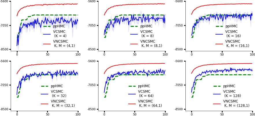
Figure 3: Log likelihood values for Vcsmc (blue) with $K$ = $\{4,8,16,32,64,128\}$ samples and Vncsmc (red) with $K=\{4,8,16,32,64,128\}$ and $M=1$ samples on the primates data averaged across 5 random seeds. Higher values of $K$ produce tighter ELBO / larger log likelihood values with lower stochastic gadient noise. Vcsmc with $K\geq 16$ outperforms probabilistic path Hamiltonain Monte Carlo ($ppHMC$) which is shown (green trace) for comparison. Vncsmc requires fewer epochs than Vcsmc to converge and produces tighter ELBO / larger log likelihood values with lower stochastic gadient noise. Vncsmc with $(K,M)=(4,1)$ (top left) outperforms both $ppHMC$ and Vcsmc with $K=128$ (bottom right).

(a) MrBayes phylogeny

(b) Vncsmc phylogeny

Figure 4: MrBayes vs Vncsmc phylogeny on the primate mitochondrial DNA dataset. The data consists of 12 taxa $\{S_{0},\cdots,S_{11}\}$ over 898 sites on the genome. The maximum likelihood topology returned by Vncsmc corresponds to that of Mr Bayes. The bottom clade partitions monkeys, while the central and top clades partition hominids and prosimians. MrBayes uses 20,000 iterations of Mcmc in contrast to Vncsmc which uses 256 samples.

5 Experiments

We evaluate Vcsmc and Vncsmc on three tasks: (i) a standard dataset of primate mitochondrial DNA, (ii) on the complete 36 kilobase genomes of 17 species of Betacoronavirus, and (iii) on 7 large taxa benchmarks datasets ranging from 27 to 64 taxa. For experiments using the same initialization of likelihood and prior, the proposed methods converge to higher log-marginal likelihood values than existing methods. Additionally, they can be more easily adopted to a variety of models, with arbitrary settings of parameters $\theta$. Vcsmc and Vncsmc also scale well with the number of sites in input sequences.

Table 1: Log-marginal likelihood estimates of different variational inference techniques across 7 benchmark datasets for Bayesian phylogenetic inference. Results reported by Vbpi [Zhang and Matsen IV, 2019] and Vbpi-Nf [Zhang, 2020] were obtained by (i) using 10 replicates of 10,000 maximum likelihood bootstrap trees  [Minh et al., 2013] to obtain topologies defining the support of the conditional probability tables and (ii) performing 400,000 parameter updates. Vcsmc does not require bootstrapped or Mcmc tree topologies in order to learn parameters. We give Vcsmc 2048 particles and evaluate the likelihood after 100 parameter updates. Results for Vcsmc and Vcsmc (JC) are averaged over three random seeds. Vcsmc consistently explores higher probability phylogenies than Vbpi and Vbpi-Nf without the use of preloaded topologies.

Log Marginal Likelihood
Dataset	Reference	# Taxa $(N)$	# Sites $(S)$	Vbpi	Vbpi-Nf	Vcsmc	Vcsmc (JC)
DS1	Hedges et al. [1990]	27	1949	-7108.4	-7108.4	-5929.8	-6906.7
DS2	Garey et al. [1996]	29	2520	-26367.7	-26367.7	-14160.4	-23252.6
DS3	Yang and Yoder [2003]	36	1812	-33735.1	-33735.1	-17460.5	-33177.8
DS4	Henk et al. [2003]	41	1137	-13329.9	-13329.9	-11251.9	-12232.6
DS5	Lakner et al. [2008]	50	378	-8214.5	-8214.5	-5797.1	-7921.2
DS6	Zhang and Blackwell [2001]	50	1133	-6724.3	-6724.3	-5216.5	-6575.5
DS7	Rossman et al. [2001]	64	1008	-8650.6	-8650.4	-5847.5	-6781.5

Primate Mitochondrial DNA.

We evaluate Vcsmc on a benchmark dataset of nucleotide sequences of homologous fragments of primate mitochondrial DNA [Hayasaka et al., 1988]. The dataset consists of 12 taxa $\{S_{0},\cdots,S_{11}\}$ over 898 sites admitting 13,749,310,575 distinct tree topologies. The set of taxa includes five species of homonoids, four species of old world monkeys, one species of new world monkey and two species of prosimians. Vcsmc is run with $K=\{4,8,16,32,64,128\}$ particles, whereas Vncsmc is run with $K=\{4,8,16,32,64,128\}$ and $M=1$ particles, each averaged over 5 random seeds. Fig. 3 shows higher values of $K$ produce larger log-marginal likelihood values (tighter ELBO values) with lower stochastic gradient noise. Vcsmc (blue) with $K\geq 16$ outperforms probabilistic path Hamiltonain Monte Carlo ($ppHMC$) shown (green trace) for comparison. Vncsmc (red) requires fewer epochs than Vcsmc to converge and produces tighter ELBO / larger log-marginal likelihood values with lower stochastic gadient noise. Vncsmc with $(K,M)=(4,1)$ (top left) outperforms both $ppHMC$ and Vcsmc with $K=128$ (bottom right).

Fig. 4 provides a single maximum likelihood phylogeny selected from a run of Vncsmc using $K,M=(256,1)$ particles, along with a phylogeny from Mr Bayes on the same dataset. The topology returned by Vncsmc corresponds to that of Mr Bayes. The bottom clade partitions monkeys, while central and top clades partition hominids and prosimians respectively.

Betacoronavirus Data.

The evolutionary origin of Sars-CoV-II and the development of its genetic variants is an open question of paramount importance in both virology and in public health. At a high level, the species Sars-CoV-II belongs to the genera of betacoronaviruses, which include Oc43 and Hku1 (which cause the common cold) of lineage A, Sars-CoV and Sars-CoV-II (which causes the disease Covid-19) of lineage B, and Mers-CoV-II (which causes the disease Mers) of lineage C [Boni et al., 2020]. The exact origin of Sars-CoV-II however is unknown; different approaches to phylogenetic inference produce statistically incompatible results [Pipes et al., 2020]. Coronaviruses have relatively large genomes ranging from 26-32 kilobases, and performing analyses on the full genomes is often a challenge. Recently, it has been argued that viral recombination in betacoronaviruses often encompasses the receptor binding domain (Rbd) of the spike gene [Patiño-Galindo et al., 2020]. This process is thought to have produced a recombination event at least 11 years ago in an ancestor of Sars-CoV-II [Patiño-Galindo et al., 2020]. We use Vncsmc to analyze the complete genomes for 17 species of Betacoronavirus downloaded from the NCBI Viral Genomes Resource [Brister et al., 2014]. Multiple Sequence Aligmnent using Clustal was performed and each nucleotide was one-hot encoded as a vector, producing input sequences with 36,889 sites. Fig. 6 of the Appendix provides the maximum likelihood phylogeny from a Vncsmc run using $K,M=(256,1)$ particles. The result shows that the phylogeny partitions four lineages into clades: Embecovirus (lineage A), Sarbecovirus (lineage B including Sars-CoV and Sars-CoV-II), Merbecovirus (lineage C), and Nobecovirus (lineage D) [Cotten et al., 2013, Woo et al., 2010, Geldenhuys et al., 2018].

Large Taxa Benchmarks.

We evaluate Vcsmc on 7 large benchmark datasets for Bayesian phylogenetic inference [Hedges et al., 1990, Garey et al., 1996, Yang and Yoder, 2003, Henk et al., 2003, Lakner et al., 2008, Zhang and Blackwell, 2001, Rossman et al., 2001]. Each dataset ranges from 27 to 64 eukaryote species with 378 to 2520 sites. Table 1 provides the marginal likelihood values for various methods. Vbpi [Zhang and Matsen IV, 2019] and Vbpi-Nf [Zhang, 2020] both learn a simplified model of molecular evolution referred to as Jukes-Cantor (JC), which fixes the transition matrix [Jukes and Cantor, 1969]. For a fair comparison, we report Vcsmc (JC) results in addition to the harder task of also learning the transition matrix. Results reported by Vbpi and Vbpi-Nf were obtained by (i) using 10 replicates of 10,000 maximum likelihood bootstrap trees  [Minh et al., 2013] to obtain topologies defining the support of the conditional probability tables and (ii) performing 400,000 parameter updates. Without bootstrap trees, the conditional probability tables for Vbpi and Vbpi-Nf scale exponentially with the number of taxa [Zhang and Matsen IV, 2019]. Vcsmc does not restrict the support of the tree topologies and instead leverages Csmc to compute a lower bound. We give Vcsmc 2048 particles and evaluate the likelihood after 100 parameter updates, averaged over three random seeds. Both Vcsmc and Vcsmc (JC) explore higher probability spaces than Vbpi and Vbpi-Nf.

Empirical Running Times.

We report the empirical running times of Vcsmc and Vncsmc on the primates dataset and highlight the results in Table 2 of the Appendix. Experiments were performed on a 2.4GHz 8-core Intel i9 processor Macbook pro with 64 GB memory and no GPU utilization. We note that alternative methods are designed for solving simpler problems in both inference and learning making any runtime comparisons indirect. For instance, Vbpi and Vbpi-Nf use precomputed topologies, while $ppHMC$ support Jukes-Cantor models. Vcsmc runs on the primates dataset at an average speed of 19.34 iterations per second (it/s) with $K$ = 4 and an average of 2.25 seconds per iteration (s/it) with $K$ = 256. Vncsmc runs in 3.89 seconds per iteration with $K$ = 4 and 21.77 seconds per iteration with $K$ = 256. These numbers can be improved by leveraging GPU utilization. In contrast, MrBayes in Figure 4 takes 12 seconds with 20,000 iterations, and the minimum it would take to converge on the primates dataset is $\sim$2,000 iterations, implying a runtime of $\sim$1.2 seconds. We observe that the first epoch of Vcsmc and Vncsmc is equivalent to the inference task and runs faster than MrBayes.

6 Discussion

Computational Complexity.

The locally optimal proposal in Ncsmc requires additional computational complexity to marginalize the intermediate target densities in exchange for a more informed exploration of partial states. Ncsmc costs $\mathcal{O}(KN^{3}M)$ in contrast to $\mathcal{O}(KNM)$ for Csmc. Empirically, Ncsmc with small $K,M$ produces a more accurate posterior approximation than Csmc with larger $K$ (see Fig. 3). Ncsmc can accommodate a large number of particles with low memory overhead, however maintaining the computational graph and applying the sum-product algorithm symbolically for each of the $K$ samples and $M$ sub-samples, along with evaluating gradients for each of these terms places a practical restriction on the values of $K,M$ and $N$ used with Vncsmc without GPU utilization. Alternative implementations of Bayesian phylogenetic inference are computationally intensive. While the process of enumerating the ${N-r\choose 2}$ topologies across rank events cannot be avoided, we find that choosing $K$ as large as possible and $M=1$ is a useful heuristic for producing good results. For example, $K,M=(256,1)$ can be run on the betacoronavirus data with $N=17$ and 36,889 sites (see Fig. 6) without GPU utilization. One advantage of Vcsmc and Vncsmc is the ability to use minibatch iteration to speed up training. The experiments were trained using Adam with a batch size $B=S/4$. Opportunities exist to parallelize Vcsmc and leverage GPU optimization which we expect would produce significant performance gains on DS1-DS7 as $K$ increases.

Effective Sample Size.

One pertinent theoretical question concerns the relationship between the effective sample size (Ess), the number of samples $K$ and the number of taxa $N$. The Ess measures the diversity among samples and is defined as $\textsc{Ess}=(\sum_{i}w_{i})^{2}/\sum_{i}w_{i}^{2}$ where $w_{i}$ are the unnormalized weights. We report Ess values on the primates data in Table 2 of the Appendix. While an Ess close to $K$ is not sufficient to ensure a good approximation, it is a necessary condition. We find near optimal Ess values across all choices of $K$ for both Vcsmc and Vncsmc. The theoretical foundations for developing lower bounds on Ess for a given value of $K$ have only been developed in the context of online inference, where the posterior distribution is updated as new sequence data becomes available [Dinh et al., 2017b]. We leave theoretical questions of Ess and online extensions of Vcsmc for future work.

Contacts Outside of Phylogenetic Inference.

Vcsmc and Vncsmc may be adapted to a wide class of problems outside of phylogenetic inference. In principle, any generative model of data simulated by a Markov tree can be fit using Vcsmc and Vncsmc. Coalescent models for heirarchical Bayesian clustering and diffusion trees [Teh et al., 2009, Boyles and Welling, 2012, Knowles and Ghahramani, 2011] are examples of alternative probabilistic approaches involving distributions over latent trees that may be suited for Vcsmc. The nested Csmc algorithm may also be used to simulate approximate solutions to other combinatorial optimization tasks. Combinatorial Monte Carlo methods are used to approximate the number of self-avoiding random walks on the lattice [Sokal, 1996, Shirai and Kikuchi, 2013]. Another point of contact is the reconstruction of jet structures in particle physics for the analysis of data from experiments at the Large Hadron Collider at CERN [Höche, 2014]. Jet reconstruction algorithms are typically based on greedy approximation methods [Cacciari et al., 2008, Dokshitzer et al., 1997], however Vcsmc and Vncsmc may be particularly suited for this domain. The aforementioned extensions are open directions for further development.

Conclusion.

We have introduced Vcsmc, a powerful framework for both inference and learning in Bayesian phylogenetics. Vcsmc is the first method to establish the use of variational sequential search to learn distributions over intricate combinatorial structures, uncovering connections between Vi and Smc. We have introduced Ncsmc, and proved that it provides an exact approximation to the locally optimal proposal for Csmc. We have used Ncsmc to define a second objective, Vncsmc which yields tighter lower bounds than Vcsmc. Vcsmc and Vncsmc outperform existing methods on a range of tasks. A TensorFlow implementation of both Vcsmc and Vncsmc is available online at https://github.com/amoretti86/phylo.

Appendix

Algorithm 2 Combinatorial Sequential Monte Carlo

  Input: $\mathbf{Y}=\{Y_{1},\cdots,Y_{M}\}\in\Omega^{NxM}$, $\theta=(\mathbf{Q},\{\lambda_{i}\}_{i=1}^{|E|})$

1:  Initialization. $\forall k$, $s_{0}^{k}\leftarrow\perp$, $w_{0}^{k}\leftarrow 1/K$.

2:  for $r=0$ to $R=N-1$ do

3:     for $k=1$ to $K$ do

4:        Resample

$$\mathbb{P}(a_{r-1}^{k}=i)=\frac{w_{r-1}^{i}}{\sum_{l=1}^{K}w_{r-1}^{l}}$$

5:        Extend partial state

$$s_{r}^{k}\sim q(\cdot|s_{r-1}^{a_{r-1}^{k}})$$

6:        Compute weights

$$w_{r}^{k}=w(s_{r-1}^{a_{r-1}^{k}},s_{r}^{k})=\frac{\pi(s_{r}^{k})}{\pi(s_{r-1}^{a_{r-1}^{k}})}\cdot\frac{\nu^{-}(s_{r-1}^{a_{r-1}^{k}})}{q(s_{r}^{k}|s_{r-1}^{a_{r-1}^{k}})}$$

7:     end for

8:  end for

9:  Output: $s_{R}^{1:K}$ , $w_{1:R}^{1:K}$

The proposal distribution for Csmc and approximate posterior for Vcsmc can be written explicitly as follows:

$$Q_{\phi,\psi}\left(\mathcal{T}_{1:R}^{1:K},\mathcal{B}_{1:R}^{1:K},a_{1:R-1}^{1:K}\right)\coloneqq\left(\prod\limits_{k=1}^{K}q_{\phi}(\mathcal{T}_{1}^{k})\cdot q_{\psi}(\mathcal{B}_{1}^{k})\right)\cdot\prod\limits_{r=2}^{R}\prod\limits_{k=1}^{K}\left[\frac{w_{r-1}^{a_{r-1}^{k}}}{\sum_{l=1}^{K}w_{r-1}^{l}}\cdot q_{\phi}\left(\mathcal{T}_{r}^{k}|\mathcal{T}_{r-1}^{a_{r-1}^{k}}\right)\cdot q_{\psi}\left(\mathcal{B}_{r}^{k}|\mathcal{B}_{r-1}^{a_{r-1}^{k}},\mathcal{T}_{r-1}^{a_{r-1}^{k}}\right)\right].$$ (16)

State $s_{r}^{k}=(\mathcal{T}_{r}^{k},\mathcal{B}_{r}^{k})$ is sampled by proposing forest $\mathcal{T}_{r}^{k}\sim q_{\phi}(\cdot|\mathcal{T}_{r-1}^{a_{r-1}^{k}})$ and branch lengths $\mathcal{B}_{r}^{k}\sim q_{\psi}(\cdot|\mathcal{B}_{r-1}^{a_{r-1}^{k}},\mathcal{T}_{r-1}^{a_{r-1}^{k}})$ from Uniform and Exponential distributions corresponding to Eq. 1 with $\phi$ and $\psi$ denoting discrete and continuous terms.

Figure 5: Overview of the Ncsmc framework. The enumerated topologies for state $\{A,B,\{C,D\}\}$ are (top): $\{A,\{B,\{C,D\}\}\}$, (center): $\{\{A,B\},\{C,D\}\}$ and (bottom): $\{B,\{A,\{C,D\}\}\}$ . $M=1$ sub-branch lengths are sampled for each edge. Sub-weights or potentials are computed (right). A single candidate is sampled to form the new partial state.

Figure 6: Overview of the betacoronavirus results. The data consists of 17 species of betacoronavirus across 36,889 sites. Vncsmc is run using $K,M=(256,1)$. A single nonclock phylogeny is chosen based on maximum likelihood and displayed. Colors denote species from the four varying viral lineages: Embecovirus (orange lineage A); Nobecovirus (blue lineage D); Sarbecovirus (red lineage B including Sars-CoV and Sars-CoV-II); Merbecovirus (grey lineage C) and Hibecovirus (black not classified into the four lineages) are each partitioned in clades.

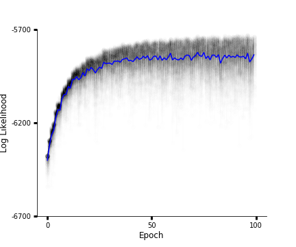
Figure 7: Vncsmc on the primates data with $K,M$ = (128, 1). The full distribution of log likelihood values for all particles across epochs is plotted in black. The average likelihood across samples is plotted in blue.

		Vcsmc				Vncsmc
$K$	s/it	s/mit	time (minutes)	Ess	s/it	s/mit	time (minutes)	Ess
4	5.17e-2	1.31e-2	0:22	3.98	4.01	1.17	6:32	3.99
8	5.58e-2	1.42e-2	0:28	7.96	4.27	1.24	7:09	7.88
16	3.11e-2	7.76e-2	0:30	15.79	4.83	1.53	8:15	15.62
32	5.78e-2	2.17e-1	0:49	31.72	5.98	1.59	10:17	31.00
64	9.80e-2	2.66e-1	1:23	62.92	8.33	2.09	14:33	62.59
128	1.35	3.48e-1	2:16	122.79	11.88	2.89	20:02	124.23
256	2.25	5.95e-1	3:52	252.02	21.77	4.98	36:51	252.43

Table 2: Empirical running times of Vcsmc and Vncsmc. The Primates data consists of 12 taxa over 898 sites admitting 13,749,310,575 distinct tree topologies. Experiments were performed on a 2.4GHz 8-core intel i9 processor Macbook Pro with 64 GB memory and no GPU utilization. We profile using $K=\{4,8,16,32,64,128,256\}$ and $M=1$. The left column provides seconds per iteration (s/it), the left center column provides seconds per minibatch (s/mit), the center right column provides total running time (minutes) across 100 epochs. The effective sample size is provided in the right columns.

Figure 8: Overview of the dual representation of a partial state. The partial state $s_{1}^{1}=\{P_{AB},C,D\}$ for four taxa corresponding to Fig. 2 is illustrated using its dual representation $\mathcal{D}(s)$. The dual state $\mathcal{D}(s)\subseteq\mathcal{T}$ corresponds to the three complete tree topologies. (left): $\{\{A,B\},\{C,D\}\}$ (center): $\{\{A,B\},\{A,B,C\}\}$ and (right): $\{\{A,B\},\{A,B,D\}\}$.

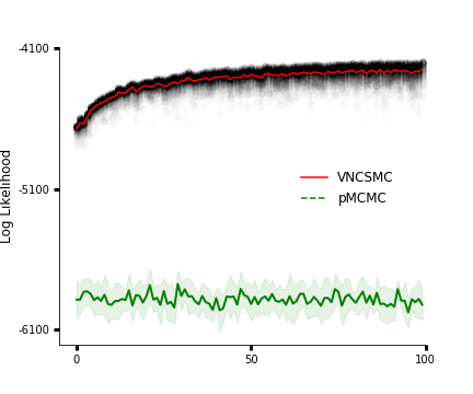
Figure 9: Vncsmc on the 9-taxa subset of primates data with $K,M$ = (128, 1). The full distribution of log likelihood values for all Vncsmc particles across epochs is plotted in black. The average likelihood across samples is plotted in red. Particle Gibbs [Wang and Wang, 2020] is run for 5000 iterations 10 times independently. The last 100 iterations for the 10 independent runs of Particle Gibbs are averaged and plotted in green. Vncsmc using 100 epochs outperforms Particle Gibbs using 5000 iterations.