GRAVITAS: Graphical Reticulated Attack Vectors for Internet-of-Things Aggregate Security

Abstract

Internet-of-Things (IoT) and cyber-physical systems (CPSs) may consist of thousands of devices connected in a complex network topology. The diversity and complexity of these components present an enormous attack surface, allowing an adversary to exploit security vulnerabilities of different devices to execute a potent attack. Though significant efforts have been made to improve the security of individual devices in these systems, little attention has been paid to security at the aggregate level. In this article, we describe a comprehensive risk management system, called GRAVITAS, for IoT/CPS that can identify undiscovered attack vectors and optimize the placement of defenses within the system for optimal performance and cost. While existing risk management systems consider only known attacks, our model employs a machine learning approach to extrapolate undiscovered exploits, enabling us to identify attacks overlooked by manual penetration testing (pen-testing). The model is flexible enough to analyze practically any IoT/CPS and provide the system administrator with a concrete list of suggested defenses that can reduce system vulnerability at optimal cost. GRAVITAS can be employed by governments, companies, and system administrators to design secure IoT/CPS at scale, providing a quantitative measure of security and efficiency in a world where IoT/CPS devices will soon be ubiquitous.

1 Introduction

Internet-of-Things (IoT) refers to any system that comprises multiple Internet-connected devices that provide transmission or computational services as one networked entity [1]. Cyber-physical systems (CPSs) employ sensor data to monitor the physical environment and create real-world change using actuators. These broad categories include systems ranging from a single Bluetooth-enabled smartwatch to a smart city containing millions of devices. Many of these devices employ rudimentary operating systems and are energy-constrained, often lacking basic security features. IoT/CPS may also consist of a diverse set of devices and complex network topologies, presenting a large attack surface that provides multiple enticing opportunities for a cunning adversary. The unique IoT/CPS exploits require that organizations employ rigorous threat analysis and risk mitigation techniques to minimize the likelihood of a successful attack.

Organizations are projected to have spent $742 billion USD on IoT devices in 2020 alone $-$ an amount which is expected to increase by 11.3% annually through 2024 [2]. Over the next few years, we can expect to see IoT/CPS move beyond small-scale applications and become significantly more commonplace in healthcare, manufacturing, transportation, law enforcement, and energy distribution [1, 3, 4, 5, 6, 7, 8, 9]. The development of 5G communication infrastructure, autonomous vehicles, and hardware specifically designed for machine learning (ML) is also accelerating the adoption of large-scale IoT/CPS [10].

However, many industry experts and leading political figures argue that the widespread adoption of IoT systems has the potential to engender “catastrophic” consequences [11, 12, 13]. One ominous sign is the Mirai botnet attack of 2016, a distributed denial-of-service (DDoS) attack that briefly brought down large parts of the Internet on the U.S. East Coast [14]. This attack was particularly notable because a single security flaw $-$ unchanged default passwords $-$ resulted in significant technological and economic disruption. This catastrophic outcome highlights how a single malicious adversary can potentially compromise an entire IoT/CPS, if not the whole Internet [14].

Cyber attacks like the Mirai botnet should serve as a warning: every IoT/CPS must be scrutinized for exploit pathways before deployment. The large attack surface of autonomous vehicle networks, smart cities, and other publicly-accessible IoT/CPS should draw particular scrutiny because a security breach of at least one connected device during the lifetime of the system is extremely likely, potentially allowing the adversary to wreak havoc on other parts of the system. It is not uncommon for multiple devices in an IoT system to have various vulnerabilities. An attacker can utilize these vulnerabilities to launch multi-stage attacks. In multi-stage attacks, a compromised device can be used as a stepping stone to attack other devices in the network. In order to prevent future Mirai-like attacks, engineers will need to take into account not just the security of individual devices, but of the system as a whole.

Moreover, securing IoT/CPS is challenging because of the limited resources available to their constituent devices. Such limitations often preclude the devices from employing intrusion detection mechanisms and executing complex cryptographic protocols. Although IoT-friendly lightweight protocols exist  [15, 16], it is still challenging to select a suitable combination of defenses to obtain optimal performance and security of the system. The high cost of adding defenses to large IoT/CPS is a frequent obstacle in deploying security features, making it critical for organizations to maximize risk reduction given a limited security budget.

Our model, called GRAVITAS, overcomes these challenges by combining the hardware, software, and network stack vulnerabilities of a system into a single attack graph. This attack graph, which includes undiscovered vulnerabilities and the connections between them as predicted by the SHARKS ML model [17], contains attack vectors that are passed over by risk management tools that employ only known vulnerabilities. These attack vectors are then assigned risk scores according to a probabilistic method that models the interaction between attack impacts and the graph’s vulnerabilities. Using these quantitative scores as a foundation for measuring risk, GRAVITAS suggests defenses to the system using an optimization process that lowers the risk score at minimum cost. With an IoT/CPS design and threat model as input, and a list of the most cost-effective defenses as output, GRAVITAS presents a security model that allows the system administrator to discover new attack vectors and proactively design secure IoT/CPS both pre- and post-deployment.

The novelty of the proposed methodology lies in:

• An automated IoT/CPS-specific exploit discovery tool that includes potential vulnerabilities and attack vectors that have yet to be discovered.

• A novel exploit scoring system that uses the topology of vulnerabilities in the attack graph to gauge risk at both the exploit and device levels.

• The ability to suggest the most effective defenses at an optimal cost via an optimization algorithm tailored to the threat model.

The article is organized as follows. Section 2 describes related work that informs this article. Section 3 presents background material on our threat model and the ML-generated attack graph that serves as the foundation for GRAVITAS, as well as a primer on attack graphs and the Common Vulnerability Scoring System (CVSS). Section 4 provides a brief description of how GRAVITAS provides novel capabilities to IoT/CPS administrators. Section 5 gives details of our methodology, including the inputs and model outputs. Section 6 provides a practical example of the model’s functionality. Section 7 includes a discussion and ideas for future work. Section 8 concludes the article.

2 Related Work

Most IoT-related security research to date has focused on remediating device-specific or application-specific security vulnerabilities. Over the last decade, researchers have discovered eavesdropping on implanted medical devices, “outage” attacks on IoT systems in nuclear power plants, tampering with smart home devices, identity theft using corrupted RFID tags, and poisoning ML models by changing sensor data, among many others [18, 19, 20, 21, 22]. This research also occurs in the corporate world: IBM, like several other companies that offer a cloud-based IoT platform, operates a lab specifically dedicated to pen-testing of IoT systems; the company claims that its laboratory has discovered over 1000 new vulnerabilities since 2017 [23]. While databases such as the National Vulnerability Database (NVD) keep track of IoT/CPS device vulnerabilities, the sheer speed with which new devices are being deployed has made up-to-date vulnerability cataloging all but impossible.

As a result, traditional exploit discovery and risk management engines are often incapable of properly modeling exploits in IoT/CPS networks. While some models have attempted to correct this problem by adapting the vulnerability scoring system or automatically-generating access conditions [24, 25], none consider the unique (and often undiscovered) vulnerabilities of public-facing IoT/CPS devices or the convoluted exploits available to a clever adversary. Even “premium” commercial risk management applications such as Tenable only examine risk from the perspective of individual vulnerabilities, rather than the chain of vulnerabilities through multiple devices that often constitute exploits in IoT/CPS [26]. While some open-source risk management systems like MulVAL can theoretically find vulnerability chains in large systems, they do not model the undocumented (yet surprisingly common) vulnerabilities present in IoT/CPS and the topology-specific connections between them [27].

GRAVITAS is also unique among IoT/CPS exploit discovery software in allowing the user to minimize the impact of a successful exploit and automatically optimize the placement of defenses to reduce risk at a minimum cost. Commercial software like Tenable claims to do risk optimization, but only does this at the vulnerability level and does not consider exploit chains between multiple devices [26]. Other tools, such as TAG and VSA, claim to have optimization abilities, but disclose very little detail in their respective articles [28, 24]. The information that does exist suggests that the available defenses for both these systems are few in number and extremely generic, bearing little resemblance to the transparent and mathematically-rigorous optimization algorithm applied by GRAVITAS. Table I compares the features of GRAVITAS to similar exploit discovery and risk management software.

TABLE I: Exploit discovery model comparison

Model	1	2	3	4	5	6	7	8	9	10
GRAVITAS	✓	✓	✓	✓	✓	✓	✓	✓	✓	✓
MulVAL [27]	✗	✓	✗	✓	✗	✗	✓	✗	✗	✗
TVA [29]	✓	✗	✗	✓	✗	✗	✓	✗	✓	✗
TAG [28]	✗	✓	✗	✓	✗	✓	✓	✓	✓	✗
A2G2V [25]	✗	✓	✗	✗	✗	✗	✓	✗	✗	✓
VSA [24]	✓	✗	✓	✗	✗	✓	✓	✗	✓	✓
Tenable [26]	✗	✗	✓	✓	✓	✓	✓	✓	✓	✗
NetSPA [30]	✗	✓	✗	✓	✗	✗	✓	✗	✗	✗

The various columns in Table I are described next.

1. Includes vulnerabilities due to physical manipulation, as well as the hardware and software stacks.

2. Discovers novel attack vectors.

3. Calculates exploit risk based on experimentally-validated algorithm.

4. Models different privileges within devices and their ability to access other devices.

5. Incorporates novel attack vectors that have not yet been exploited in real-world systems.

6. Optimizes defense placement to reduce exploit risk at minimum cost.

7. Can find “the weakest link” (most vulnerable part of the system).

8. Accurately handles cyclic network topology.

9. Allows easy customization based on a system administrator’s risk impact assessment and chosen adversary model.

10. Designed specifically for the unique characteristics of IoT/CPS networks.

3 Background

GRAVITAS employs several concepts developed in previous exploit detection frameworks. These include the SHARKS IoT/CPS model, attack graphs, and the CVSS metrics for evaluating the impacts of vulnerabilities. This section provides an introduction to these concepts.

3.1 The SHARKS Framework

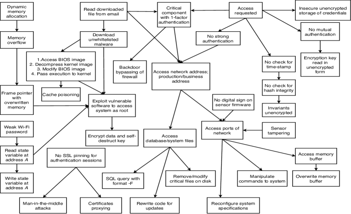
Figure 1: The original SHARKS attack graph [17]

GRAVITAS builds on the work of SHARKS (Smart Hacking Approaches for RisK Scanning in Internet-of-Things and Cyber-Physical Systems based on Machine Learning), which provides a novel framework for discovering IoT/CPS exploits [17]. Instead of artificially separating a system into different layers, SHARKS eschews a rigid classification and models an exploit chain (attack vector) as it appears to an adversary: a series of steps that begins at an “entry point” (a root node) and ends at a “goal” (a leaf node). The SHARKS attack graph (Fig. 1) was created by deconstructing 41 known attacks on IoT/CPS into a series of steps represented by a vulnerability node chain (an exploit), and subsequently merging every node chain into a single directed acyclic graph (DAG). This graph makes no distinctions between network-level, hardware-level, or software-level nodes: what matters is the procedure that brings attackers to their desired destination.

SHARKS assigns descriptive features to each node in the attack graph, using one-hot encoding for categorical features as well as using continuous features such as the node’s mean height in the graph. The authors assign a target feature to each pair of nodes indicating whether the two were connected by an edge (an ordered sequence of two steps in an attack). This dataset is then used to train a Support Vector Machine (SVM) model, which discovered 122 novel exploits.

3.2 Attack Graphs

Both SHARKS and GRAVITAS are based on attack graphs, albeit with minor differences in their node types. We describe each graph ($G$) using the following terminology:

• $N$: The set of nodes in the graph. Each node represents a single vulnerability in the system, such as “sensor tampering” or “no SSL pinning.”

• $E$: The set of edges in the graph. Edges represent exploits, or pathways between vulnerabilities. Unlike in other attack graph models, edges do not have an access control parameter; each edge instead represents a possible path between vulnerabilities. Different permissions are instead represented by different nodes (see Section 5.2.2).

• $D$: The set of nodes and edges corresponding to one device. Every device is depicted by a subgraph of the complete attack graph ($D\subset G$).

• $A$: The nodes at which an adversary can access the system. These “entry nodes” are the starting points for any attack. They are also vulnerabilities ($A\subset N$).

• $L$: The leaf nodes of the graph. These represent the completion of an attack ($L\subset N$). These “exploit goals” represent the end goal of an adversary’s attack, such as ”Disable device” or ”DoS attack.”

• $P$: The set of nodes that constitute a complete attack vector. Each exploit begins at an entry node and concludes at an exploit goal node. More formally, an exploit $P$ is any ordered set of nodes in the form $\{a,n_{1},...,n_{k},l\}$ where $a\in A$, $n_{i}\in N$, $l\in L$. The same entry node and exploit goal pair can be a part of multiple attack vectors.

• $M$: The set of all defenses that can be applied to the attack graph.

• $\widetilde{M}$: The subset of defenses chosen by the optimization process.

3.3 Common Vulnerability Scoring System (CVSS)

CVSS is an experimentally-validated scoring system for device vulnerabilities that is widely used in risk management systems [31]. In this article, every node in the attack graph is assigned a vulnerability score, which represents the intrinsic risk of the vulnerability to the system. This score incorporates both the impact of a vulnerability and its ease of exploitation, and is calculated using an algorithm almost identical to that used in CVSS to score vulnerabilities (see Section 5.3.1). This algorithm uses the scoring factors described in Table II. There are three principal categories of factors: exploitability, impact, and defense. Exploitability refers to the effort required by an adversary to “succeed” in an attack step, while impact refers to the damage that a successful attack can inflict on the security of the system. Defense refers to the extent to which the attack is prevented from being exploited. The scores in the exploitability category are determined by the composition of the attack graph and are computed algorithmically, while those for impact are decided by the system administrator based on their judgement of an attack’s impact. The defense scores are hard-coded to the particular defense, though these can be modified by the user. In Table II, the scores marked with a * are taken from a study by Ur-Rehman et al. that adapts some of the original CVSS scores to better reflect the ease of exploitation of real-world IoT/CPS devices [24]. The scores marked with a $\dagger$ are newly-added scores that have been experimentally validated using the method described in Section 5.6.

TABLE II: CVSS scoring values [31]

Category	Factor	Type	Score
Exploitability	Attack vector	Network	0.85
		Adjacent	0.62
		Local	$0.60^{*}$
		Physical	$0.44^{*}$
	Attack complexity	Low	0.77
		Medium	$0.44^{*}$
		High	$0.20^{*}$
	Scope	Changed	N.A.
		Unchanged	N.A.
	Privileges required	None	0.85
		Low; Scope Changed	0.68
		Low; Scope Unchanged	0.62
		High; Scope Changed	0.50
		Low; Scope Unchanged	0.27
	User interaction	None	0.85
		Required	0.62
	Accessibility	High	$0.80^{\dagger}$
		Medium	$0.60^{\dagger}$
		Low	$0.40^{\dagger}$
		None	$0^{\dagger}$
Impact	Confidentiality	High	0.56
	Integrity	Low	0.20
	Availability	None	0
Defense	Node & edge defense	None	$1^{\dagger}$
		Workaround	$0.90^{\dagger}$
		Temporary	$0.60^{\dagger}$
		Definite	$0.30^{\dagger}$
		Infallible	$0^{\dagger}$

3.4 Threat Model

Our threat model consists of an adversary who wishes to achieve an exploit goal $l$ with a motivation specified by its impact score. The adversary reaches the desired $l$ by starting at an entry node $a$ and passing through other vulnerability nodes $n_{i}\in N$. This complete path $P$ is known as an exploit chain or attack, and may involve vulnerabilities in multiple devices (see Section 6 for an example). While the system administrator can assign a unique impact score to each $l$ or randomly assign the scores via a specified distribution, it is not known in advance which exact exploit goal an adversary may attempt to access. Hence, the administrator must take into account all possible exploits in the attack graph in order to minimize risk over the entire system.

For simplicity, we assume that the motivation of the adversary to inflict damage is congruent to the system administrator’s assessment of the damage that the attack would cause to system security. We also assume that the adversary also has access to GRAVITAS and may decide to perform an exploit based on information provided by the model. As a result, the system administrator has an incentive to ensure that high-impact exploits are not easily accessible to the adversary. This may require adding additional defenses to the system via the model’s optimization component.

4 Motivation

While SHARKS is able to find novel exploits on specific types of IoT/CPS, it is too generic to adequately model the multitude of intricate exploits in a real-world system. GRAVITAS solves this issue by creating a unique attack DAG for every device in an IoT/CPS and adding additional pathways between devices based on network topology. The goal is not to find specific vulnerabilities in each device (a process that often requires static and dynamic analysis of the system) but to understand the impact that an exploit would have on the security of the entire system if a certain vulnerability were to exist. Moreover, unlike other IoT/CPS security models, GRAVITAS can account for potential exploits that have not yet been discovered, enabling a proactive and comprehensive approach to network security that existing risk management tools cannot provide. GRAVITAS can also suggest defenses that reduce system vulnerability at the lowest cost, employing a “defense-in-depth” optimization approach that is intractable to human analysis. By giving an administrator the ability to visualize and mitigate IoT/CPS exploits before the system is deployed, GRAVITAS hopes to prevent the next Mirai-like attack before it happens.

5 Methodology

In this section, we describe the GRAVITAS methodology. As shown in Fig. 2, GRAVITAS consists of four primary components:

1. Deriving the device templates from SHARKS.

2. Creating an attack graph from the devices and network topology specified by the system administrator.

3. Calculating the vulnerability score and exploit risk score for every node in the graph.

4. Optimizing the placement of defenses to reduce the total exploit risk of the system.

Figure 2: The overall structure of GRAVITAS

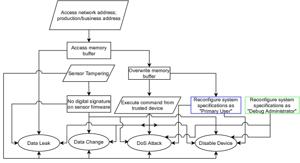
Figure 3: Nest Garden Sensor in the smart home system as derived from a template for a Sensor (Non-updatable, Send and Receive, Local Network Access). Ovals represent exploit goals and parallelograms represent entry nodes. The blue and the green nodes represent the same subgraph that is repeated for each user-specified permission (see Section 5.2.2 for more detail).

TABLE III: The exploit goals in the master attack graph template $J$

Exploit Goal	Example
Eavesdropping over network	Unencrypted communication channel allows adversary to glean information
Denial-of-Service (DoS)	Mirai botnet used to flood DNS servers with bogus traffic
Disabling device	Adversary remotely turns off a smart city drone mid-operation, causing it to crash
Actuator malfunction	IoT-enabled pacemaker told to increase pace of electric shocks, causing serious harm to the patient
Data leak	Adversary accesses memory of a smart lock, learning the times of day when the victim is not at home
Data change	Adversary gains control of a traffic sensor and provides fake data to an ML algorithm that suggests routes for autonomous vehicles
Replay attack	Communications protocol does not use a digitally signed timestamp, allowing the adversary to resend previous commands
Ransomware attack	Adversary gains root access to device and encrypts essential files, asking the user to present payment in exchange for the key
Obtain authentication key to device $i$ with permissions $j$	Adversary finds password on a mobile device that permits him to login to a local controller from a different device
Obtain open access to device $i$ with permissions $j$	Adversary finds password on a mobile device that permits him to login to a local controller directly from the mobile device

These components are described in Sections 5.1 through 5.4, respectively. Section 5.5 describes the adversary model, whereas Section 5.6 describes a quality assurance program that employs randomly-generated smart city IoT/CPS to test the robustness of the internal parameters of GRAVITAS.

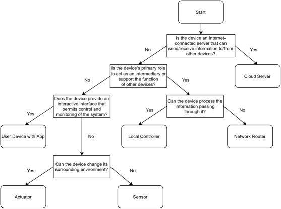
Figure 4: Flowchart for choosing the correct device category

TABLE IV: Device subcategories for template construction

Factor	Subcategory	Description	Examples
1	Non-updatable	Device’s application-level software and firmware cannot be changed	Devices with application software as immutable firmware, devices without a CPU (including some ASICs), devices without transistors or memory
	Updatable	Device’s application-level software or firmware can be changed	Any device that runs a version of Linux or most versions of RIoT, PSoC, and FPGA-like devices
2	Local network access	Device is only connected to a local network (no direct Internet access)	Fitbit Versa 2 (still considered local network access only if Internet-based data are accessed via a non-router proxy device)
	External network access	Device is connected to the Internet (this can be through an adjacent router)	Apple Watch Series 5 Cellular Model
3	Send	Device is physically capable of broadcasting a signal in a format readable to other devices	A sensor with an output port containing a pin that can vary its voltage
	Receive	Device is physically capable of receiving and “understanding” a signal from another device	An actuator with a simple electronic circuit that depends on the input voltage level
	Send and receive	Device can both send and receive information	4G-enabled smartphone, drone with camera

5.1 Deriving Device Templates

All device attack graphs used in GRAVITAS are derived in part from an updated version of the SHARKS graph. This master attack graph template ($J$) consists of a subset of the original SHARKS graph, including ML-predicted edges between nodes that indicate new vulnerabilities. Each of these templates contains all known and predicted vulnerabilities and attack vectors for a given device. By including predicted exploits rather than just publicly known exploits in the system attack graph, GRAVITAS allows the system to be protected against possible novel exploits.

Every graph $J$ also contains a new set of nodes designated as exploit goals, $L$. Table III lists the exploit goals; they collectively represent all of the IoT/CPS exploits described in [1]. In addition, we designate certain nodes from the original SHARKS graph as entry nodes, $A$. Even with these additions, the master attack graph $J$ is still a DAG, ensuring that any exploit $P$ derived from it will be finite in length and non-repeating. GRAVITAS contains dozens of different templates for IoT/CPS devices, each of which is further customizable based on user input. Fig. 3 shows an example of a device template that has been customized to a device present in the smart home example application (see Section 6 for more detail).

5.1.1 Creating the Device Templates

Every device template $T_{i}$ is a subgraph of $J$, the master attack graph ($T_{i}\subset J$). A device graph $D$ consists of the corresponding device template with modifications specified by the system administrator’s input. While each device graph $D$ derived from a template is a DAG, the complete system attack graph $G$ may contain cycles in certain network topologies. This is acceptable because the “long” cycles created by pathways between devices still permit the exploit risk score calculation process to converge in a reasonable time frame (see Section 5.3.2 for further details).

To create a device graph $D$, we must first classify the device using four factors. The first of these factors, which we refer to as a category, describes the purpose of the device; Fig. 4 shows a flowchart that helps the system administrator decide which of the six categories to select. We refer to the other three factors as subcategories, each of which describes a physical limitation of the device and consequently a hard boundary on the kind of attacks it is susceptible to. These subcategories are described in Table IV. The categories and subcategories together provide comprehensive coverage of the numerous IoT/CPS applications listed in [1].

5.2 Creating IoT/CPS Designs

Fig. 5 provides an overview of how GRAVITAS creates an attack graph $G$ from system administrator input. In addition to specifying inherent device properties, such as the device category and subcategories, the system administrator must also describe each device’s location in the network topology. This includes its connections (wired and wireless) to devices in the local network as well as its ability to connect to an external network such as the Internet. Table V describes a subset of these device-level characteristics. Note that most of these characteristics are entirely optional. Only “Name,” “Category,” and “Subcategory” are strictly necessary; all other characteristics receive default values that treat the device as a disconnected component with a low security risk. If the system administrator is unsure about the topology of a certain device or its impact scores, GRAVITAS can automatically generate the connections and impact scores from a random distribution with parameters set by the administrator. For an example of a system design, see Section 6.

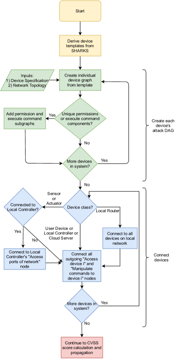
Figure 5: The procedure for creating the complete system graph $G$ from system administrator input

TABLE V: Administrator-specified device properties

Device property	Description
Name	Unique name of device
Category	Choose from the categories in Fig. 4
Subcategory	Choose from the subcategories in Table IV
Device set	Devices in the same set are treated as identical; during system optimization, all devices in a single set are given the same defense concurrently
Confidentiality scores	A list of CVSS confidentiality scores for the exploit goals of this device
Integrity scores	A list of CVSS integrity scores for the exploit goals of this device
Availability scores	A list of CVSS availability scores for the exploit goals of this device
Accessibility scores	A list of accessibility scores for the entry nodes of this device
Login permissions	A list of devices that possess credentials to login to this device; a single device may have multiple permission types, and multiple devices may login to this device using the same permission type
Execute command permissions	A list of devices that possess credentials to send valid commands to this device; a single device may have multiple permission types, and multiple devices may login to this device using the same permission type
General permissions	Some simple devices, such as embedded IoT sensors, do not possess a formal security protocol, and can be controlled by any device that connects to them
Local networked devices	A list of devices in this device’s local network; if this is a “hub” network centered around a device like a WiFi router, the algorithm will automatically connect all devices in a local network group as long as each device is connected to the hub

5.2.1 Defenses

TABLE VI: Defense properties

Defense property	Description
Defense name	Unique name for the defense; all defenses in a device set that share the same name will be applied simultaneously if chosen during optimization
Device name	A list of devices to which this defense can be applied
Cost	The cost of defense in relative units
Node score list	A list containing each node and updated node defense score affected by the defense
Edge score list	A list containing each edge and updated edge defense score affected by the defense

TABLE VII: Selected defenses in $M$ (with default settings)

Defense	Type	Vulnerability(-ies)	Cost
Multifactor authentication	Single node	No mutual authentication	2
Salt, hash, and encrypt passwords	Single node	Encryption key read from memory in unencrypted form	1
Limit installation of unverified software	Single node	Download unwhitelisted malware	1
Limit physical access to device ports	Multi node	Sensor tampering, side-channel analysis	3
Establish difficult-to-crack device passwords	Edge	Access requested, no strong authentication	2

GRAVITAS provides $M$, the set of potential defenses that can be applied during optimization. The defenses in GRAVITAS are derived from ENISA’s Baseline Security Recommendations for IoT [32]. This list includes vulnerability mitigation strategies identified in NIST, OWASP, ISO, and a variety of other standard-setting organizations. Similar to the widely-employed mitigation techniques cataloged in MITRE’s ATT&CK database [33], the defenses employed by GRAVITAS correspond to a vulnerability category (“technique”) that is present across devices in the same category. Section 6 illustrates how an optimized subset of these defenses can be applied to exploits in a real-world system. Note that the system administrator can add or subtract defenses to $M$ if additional specificity or generality is required, and also change the defense cost.

Table VI describes the properties of a defense in detail. Defenses can act at two places: nodes and edges. A node defense changes the score used in the node’s vulnerability score calculation (see Section 5.3.1). An edge defense changes the weight multiplier of the corresponding edge during exploit risk score propagation (see Section 5.3.2). The cost of each defense and its marginal improvement to the total exploit risk (adversary score) are used in the objective function that determines which defense to add (see Section 5.4.1). Table VII shows a small selection of node (vulnerability) defenses in $M$.

Every device graph $D$ initially gives each of the device’s permissions blanket access to a device’s capabilities, similar to administrator privileges. To limit the access of a certain permission, the system administrator can specify a defense that removes an edge between nodes in a permission subgraph (see Section 5.2.2). This blacklist approach simplifies the input and ensures that low-cost/high-impact defenses are added at the beginning of the optimization process.

In GRAVITAS, the cost of each defense is fixed at the outset of optimization. However, system administrators can set their own cost values based on various constraints of the system such as latency, expenditure, and energy. Because the cost and adversary score are weighted using a constant in the optimization function, the administrator can think of the cost of each defense in relative terms when deciding which values to choose. As a result, the specific numbers are not as important as the relative cost between different kinds of defenses: for example, the administrator could classify a defense’s cost as either “high,” “medium,” or “low,” each of which has a specific numerical value associated with it in a manner similar to a CVSS scoring attribute.

5.2.2 Permission Subgraphs

GRAVITAS allows the system administrator to specify permissions for every device. Unlike other attack graph models, the access permissions are each represented by a separate copy of a subgraph rather than as a logical statement at certain nodes or edges [34, 35, 36]. This design choice makes a visualization of the attack graph easier to understand, and also simplifies the calculation of exploit risk scores because we can apply the same closed-form calculation to every node-edge pair (see Section 5.3.2).

We model two different types of permissions: login permissions and execute command permissions. With a login permission, a user with the correct credentials can execute any (permitted) command on the system; this is similar to a user profile on a Linux or Windows system. With an execute command permission, a user with the correct credentials can execute a (permitted) command from a specified list. For example, this could be a set of commands recognizable in a JavaScript Object Notation (JSON) packet or the movement controls for an autonomous drone. Depending on the configuration of the IoT/CPS, different devices may have login/execute commands under the same permission name.

As described in Table VIII, certain nodes in every device template are associated with login permissions, execute command permissions, or both. These subgraphs are “repeated” for every permission type of that device. Fig. 3 shows the system-specific device graph $D$ with nodes in different permission subgraphs delineated in different colors. Note that the system administrator can specify defenses that effectively remove certain nodes or edges, allowing the administrator to set restrictions on what each permission can access.

TABLE VIII: Permission subgraph node types

Attack node	Login permission	Execute command permission
Access network address; production/business address	Yes	No
Access ports of network	Yes	No
Reconfigure system specifications	Yes	Yes
Access database/system files	Yes	Yes
SQL query with format -F	Yes	Yes
Rewrite code for updates	Yes	Yes
Remove/modify files on disk	Yes	Yes
Download unwhitelisted malware	Yes	Yes
Read state variable at address A	Yes	Yes
Write state variable at address A	Yes	Yes
Execute command	No	Yes

5.2.3 Connecting the Devices

Once every device’s attack graph $D$ has been produced, we can connect them together into an aggregate attack graph $G$ using the network topology specified by the system administrator. A login permission $j$ is represented by an edge originating from the exploit goal “Obtain authentication key to device $i$ as permission $j$,” while an execute command permission $j$ is represented by an edge originating from “Manipulate commands to device $i$ with permission $j$.” Both lead to the node “Access network address, production/business address as permission $j$” of device $i$. Both of these connections allow the devices to bypass the device’s authentication procedures, meaning that the attacker does not have to start at the “Access requested” node where almost all non-authenticated adversaries must begin their attack. For certain sensors and actuators, “Sensor tampering” and “No digital signature on sensor firmware” are connected to the “Access ports of network” node of the neighboring local controller; this represents the local network that exists between certain local controller and sensor/actuator setups, such as those involving an Arduino. To model access to a local network, every router’s “No strong authentication” node is connected in both directions to that same node in all other adjacent routers, and is also connected to the “Access requested” node for adjacent devices that are not routers. External network access (i.e., to the Internet) is modeled by including nodes such as “Download unwhitelisted malware” in the device template.

5.3 Calculating and Propagating Vulnerability Scores

Every node in the attack graph is first assigned a vulnerability score. These scores are then “propagated” through the graph, giving each attack node an exploit risk score. The total exploit risk of the IoT system or CPS, which we call the adversary score, is calculated using the adversary model chosen by the system administrator and involves a function of the exploit risk scores of entry nodes (see Section 5.5). This score is used in the objective function employed in the defense placement optimization process described in Section 5.4. The vulnerability scores are only calculated once, whereas the exploit risk scores (and adversary score) must be recalculated after adding a new defense.

All vulnerability and exploit risk scores fall into the [0,1] range. This is a departure from the traditional CVSS scoring range of [0,10], but it allows us to treat each score as the probability that an adversary will attempt the attack and succeed in exploiting it. This approach is widely used in attack graph models because it allows for a probabilistic understanding of an adversary’s movement through the graph [36, 37, 24].

5.3.1 Calculating vulnerability scores

$ISS=1-[(1-confidentiality)(1-integrity)(1-availability)(1-accessibility)]$;

if $scope$ is unchanged then

      $Impact=6.42\times ISS$;

else

       $Impact=7.52\times(ISS-0.029)-3.25\times(ISS-0.02)^{15}$;

end if

$Exploitability=8.22\times attack\_Vector\times attack\_Complexity\times privileges\_Required\times user\_Interaction$;

 if $Impact<0$ then

      $Impact=0$;

end if

if $scope$ is unchanged then

      $x=min[(Impact+Exploitability),10]$;

else

      $x=min[1.08\times(Impact+Exploitability),10]$;

end if

$vulnerability\_Score=\frac{x}{10}\times defense\_Score$

Algorithm 1 Vulnerability score calculation

Algorithm 1 describes the process for calculating the vulnerability score. This algorithm (including its constants) is identical to the experimentally-validated “Base Metrics Equations” present on page 18 of the CVSS Specification Guide, with the addition of a final line that adjusts the vulnerability score based on the defense(s) applied to the system [31].

Each node’s vulnerability score is calculated using the Exploitability factors ($scope$, $attack\_Vector$, $attack\_Complexity$, and $user\_Interaction$) described in Table II. The value of each factor is computationally determined by an algorithmic version of the corresponding flowchart on pages 20-21 of the CVSS v3.1 user guide, and is thus dependent on the node’s permission characteristics and its topographic position within the device graph $D$ [38]. The impact factors ($confidentiality$, $integrity$, and $availability$) are set by the system administrator, as is the $accessibility$ score of each entry node. These factors are used to calculate the $ISS$ (Impact Sub-Score). If the system administrator does not want to specify the impact score for every exploit goal, the scores can be auto-generated by providing parameters for the distribution of impact scores in the specified system components. This process is similar to the one used to randomly generate IoT/CPS for testing purposes (see Section 5.6 for more detail).

5.3.2 Propagating Exploit Risk Scores

To model IoT/CPS security, we need an understanding of how vulnerability scores of different nodes interact. This interaction is represented by each node’s exploit risk score, which is calculated using a function that involves the exploit risk scores of adjacent child nodes (see Algorithm 2).

An adversary generally wants to take the least risky path possible through the attack graph; consequently, the longer and more difficult the path, the less likely the adversary is to pursue it, and the lower the exploit risk score should be. In a similar fashion, we would consider an attack graph to be more vulnerable if there are multiple paths to the same exploit goal. To represent this idea in the exploit risk score calculation (Algorithm 2), we employ a probabilistic union function that gives the likelihood that an adversary will execute at least one of the exploits flowing from the current node to its children [37]. This method is effective because it incorporates the children nodes’ exploit risk scores (and the scores of their descendants, including exploit goals) into the exploit risk scores of their parents. Consequently, the exploit risk score of an entry node represents the vulnerability of all exploits reachable from that location. Section 5.6 provides a description of how the parameters and functions in this algorithm were experimentally determined.

Function $calculate\_Exploit\_Score$($n$, $G$):

       Data: Node $n$; Attack graph $G$

       Result: Exploit risk score for $n$

       // $c_{i}$ is a child of node $n$ $union\_Probability=n.vulnerability\_Score\times(1-\prod_{i=1}^{k}(1-(c_{i}\times edge\_Defense(n,c_{i}))))$;

       $exploit\_Score=-7^{-union\_Probability}+1$ ;

       /* Activation function (see Section 5.6 for more details about how this function was determined) */

      if $exploit\_Score>1$ then

            $exploit\_Score=1$;

       end if

      if $exploit\_Score<0$ then

            $exploit\_Score=0$;

       end if

      

      return exploit_Score;

Algorithm 2 Exploit risk calculation

Data: Attack graph $G$ with nodes $n_{1}$, … ,$n_{k}\in N$; entry nodes $A\displaystyle\subset N$; exploit goal nodes $L\displaystyle\subset N$

Result: Attack graph $G$ with exploit risk scores at each $n_{i}$

$average\_Sum=$ $\mid A\mid$;

while $\frac{average\_Sum}{\mid A\mid}>sum\_Ratio$ and $count<max\_Cycle$ do

       $average\_Sum=0$;

       Queue $Q\longleftarrow L$;

       while $\mid Q\mid$ $>0$ do

             $n\leftarrow Q$.dequeue;

             if $n$ has not been visited  then

                   $n.exploit\_Score=$ calculate_Exploit_Score($n$, $G$) ;

                  

                  if n $\in$ A then

                         $average\_Sum=average\_Sum+|n.exploit\_Score-n.exp\_Avg|$;

                        

                   end if

                  

                  $n.exp\_Avg=exp\_Weight\times n.exploit\_Score+(1-exp\_Weight)\times n.exp\_Avg$;

                   Mark $n$ as visited;

                  

                  for $parent\_Node$ in $n.parents$ do

                         if $parent\_Node$ has not been visited then

                               $Q$.append($parent\_Node$);

                              

                         end if

                        

                   end for

                  

             end if

            

       end while

      $count+=1$;

      

end while

Algorithm 3 Propagating exploit risk scores

If we think of each vulnerability as a neuron, we can think of the attack graph as a recurrent neural network (RNN), where the neuron-level score calculation combines inputs from multiple adjacent children nodes that are fed into an activation function. As with forward propagation in an RNN, our score propagation algorithm uses a breadth-first search that halts at nodes that have already been visited; once all nodes have been visited, we repeat the whole process and continue this repetition until the scores at the entry nodes have converged. Algorithm 3 shows this process in detail.

TABLE IX: Administrator-specified parameters for controlling the score propagation and optimization process

Parameter	Purpose	Description	Suggested values
$sum\_Ratio$	Limits number of propagation cycles in Algorithm 3 to reduce computation time	Sets a floor on the average of the difference between every entry node’s most recent exploit score and a weighted average of its exploit scores from previous propagation cycles. This difference should approach zero as the exploit scores converge.	$10^{-4}$ to $10^{-6}$
$exp\_Weight$	Helps measure progress towards the convergence of entry node exploit scores	This is the parameter for determining the exponentially-weighted moving average of a node’s exploit risk score over all propagation cycles. We compare this average to the newest score to gauge convergence.	$0.05$ to $0.2$
$max\_Cycle$	Limits number of propagation cycles in Algorithm 3 to reduce computation time	Sets a ceiling on the number of propagation cycles	$50$ to $250$
$max\_Defenses$	Limits number of optimization rounds	The maximum number of defenses that can be added during optimization	$|N|\times$[0.05 to 0.2]
$opt\_Halt\_Value$	Limits the number of optimization rounds	Sets a floor for the global objective value, below which optimization ceases	Preference-dependent
$\alpha\_Global$	The weighting for the global objective function	The weighting of $total\_Cost$ against $adversary\_Score$ increases linearly with $\alpha\_Global$	Preference-dependent
$\alpha\_Local$	The weighting for the local objective function	The weighting of $defense\_Cost$ against the marginal difference in $adversary\_Score$ increases linearly with $\alpha\_Local$	$0$ to $0.0001$
$max\_Set\_Time$	Improve optimization performance by removing low-performing defenses	The maximum amount of rounds that a defense may remain in the defense set	$10$ to $50$
$set\_Size$	Reduce computation time by comparing less defenses in every optimization round	The number of defenses in the defense set. A larger defense set will result in a better optimization result	$0.05\times|D|$ at minimum

5.4 Optimizing Defense Placement

Data: Attack graph $G$; defenses $d_{1}$, … ,$d_{j}\subset M$

Result: $H$, $h\_Best$; /* $h\_Best$ includes the optimally-defended graph $G$ and optimal defense set $\widetilde{M}\subset M$ */

$S$ = refresh_Defense_Set($\emptyset$, $G$); /* $S$ is a set containing graphs that each differ in only one defense */

$H$ $=$ $\emptyset$;

repeat

      

      $chosen\_Min\_Obj\_Val=\infty$;

       for $s$ in $S$ do

            

            $local\_Obj\_Value=$ local_Objective_Func($\alpha\_Local$, $s.d.cost$, adversary_Score($s.G$));

             if $local\_Obj\_Value$ $<chosen\_Min\_Obj\_Val$ then

                  

                  $chosen\_Set=s$;

                  

             end if

            $s.time\_In\_Set=s.time\_In\_Set+1$;

            

       end for

      $total\_Cost=total\_Cost+chosen\_Set.d.cost$;

      

      $H$.add(make_History_Moment($chosen\_Set.d$, $chosen\_Set.G$));

      

      $S$.remove($chosen\_Set$);

      

      $S=\textbf{refresh\_Defense\_Set}$($chosen\_Set.d$, $chosen\_Set.G$);

      

until $\mid S\mid$ $\leq 0$ and $\mid H\mid$ $\geq max\_Defenses$ and global_Objective_Func($\alpha\_Global$, total_Cost($h.\widetilde{M}$), adversary_Score($h.G$)) $\leq opt\_Halt\_Value$ ;

$min\_Global\_Obj\_Val=\infty$;

for $h\in$ $H$ do

      

      $global\_Obj\_Val=$ global_Objective_Func($\alpha\_Global$, total_Cost($h.\widetilde{M}$), adversary_Score($h.G$));

      

      if $global\_Obj\_Val$ $<min\_Global\_Obj\_Val$ then

            

            $min\_Global\_Obj\_Val=global\_Obj\_Val$;

             $h\_Best=h$

       end if

      

end for

Algorithm 4 Optimizing the system

The optimization component of GRAVITAS adds defenses to the system with the goal of minimizing objective functions specified by the system administrator. It does this by creating a “history” set $H$ that records the defense selections of successive optimization rounds. One ”moment” in history $h\in H$ refers to a single iteration of executing the local objective function; each $h$ includes the defense that was just chosen as well as an attack graph whose scores have been updated to include the just-chosen defense and all previously-added defenses. Once all $h$ have been determined, we use a global objective function to choose the optimal defense set $\widetilde{M}$ from among all $h$. Algorithm 4 provides an overview of the optimization algorithm, whereas Algorithm 5 describes the refresh_Defense_Set($d$, $G$) function that is used to generate the defense set $S$ whose hypothetical defense-graph pairings are compared by the local objective function. Section 5.4.1 describes the local and global objective functions in detail. Table IX describes the parameters the administrator can set to further refine the optimization process.

5.4.1 Objective Functions

Choose from all defense set members $s\in S$, where $s$ consists of a just-added defense $d$ and corresponding graph $G$.

$$\begin{gathered}\textbf{min}[\alpha\_Local\times s.d.cost+(1-\alpha\_Local)\\ \times(\emph{adversary\_Score}(h_{t-1}.G)-\emph{adversary\_Score}(s.G))]\end{gathered}$$ (1)

Choose from among all moments in history $h\in H$, where $h$ consists of defense set $\widetilde{M}$ and corresponding graph $G$ with all $d\in\widetilde{M}$ added.

$$\begin{gathered}\textbf{min}[\alpha\_Global\times total\_Cost(h.\widetilde{M})\\ +(1-\alpha\_Global)\times\emph{adversary\_Score}(h.G)]\end{gathered}$$ (2)

The purpose of each objective function is to minimize the system’s total exploit risk (adversary_Score) while simultaneously minimizing the cost of the defenses needed to lower the vulnerability. We employ two separate objective functions: local and global (Eq. (1) and (2), respectively). The local objective function is applied to every defense-graph pair in the current defense set; the pair that minimizes the objective function is added to the defense history. The global objective function is employed after the algorithm has completed populating the defense history; it chooses the optimal “moment” (cumulative set of defenses) from the history. Each function employs a user-specified parameter $\alpha$ that tells the function how to weigh the adversary score against the cost. Note that in the local objective function, we weigh the marginal increase in defense cost against the corresponding marginal decrease in the graph’s adversary score, while in the global objective function, we weigh the total cost against the current adversary score.

5.4.2 Choosing Defenses

Function refresh_Defense_Set($d$, $G$):

       Data: Defense $d$ just selected by objective function, graph $G$ with optimal defense just added

      

      for $s$ in $S$ do

            

            if $s.timeInSet>max\_Set\_Time$ then

                  

                  $S$.remove($s$);

                   $available\_Defense\_List$.add($s.defense$)

             end if

            

       end for

      

      for $G\in$ $S.graphs$ do

            

            $G$.apply_Defense($chosen\_Defense$);

             $G$.propagate_Defense($chosen\_Defense$);

            

       end for

      

      $max\_Vul\_Device\_Defenses=$ All unused defenses from the device with the highest exploit risk score;

      

      while  $\mid S\mid$ $<set\_Size$ and $\mid available\_Defense\_List\mid$ $>0$  do

            

            if $\mid max\_Vul\_Device\_Defenses\mid$ $>0$ then

                  

                  $d$ = random_Defense($max\_Vul\_Device\_Defenses$);

                  

            else

                   $d$ = random_Defense($available\_Defense\_List$);

                  

             end if

            

            $new\_G=$ deep_Copy($G$);

             $new\_G$.apply_Defense($d$);

             $new\_G$.propagate_Defense($d$); /* Similar to Section 5.3.2, except that the first nodes in the queue are the nodes upon which the new defense is placed */

             $S$.add($d$, $new\_G$);

             $available\_Defense\_List$.remove($d$);

            

       end while

      

      return $S$;

      

Algorithm 5 Refreshing the defense set

In every optimization round, we choose the defense that minimizes the value of the local optimization function: Eq. (1). The defenses that are used in this comparison are located in the Defense set $S$, a list of fixed length that contains a subset of defenses that are most likely to improve the optimization function. Every defense in $S$ is associated with a graph $G$ that contains that same defense and all the defenses already applied to $G$. This list is managed via Algorithm 5, which is invoked to refresh the defense set after every optimization round.

A defense may be removed from $S$ for two reasons: either it has already been selected as the optimal defense in the previous optimization round, or it has been in the set for too many optimization rounds (longer than $max\_Set\_Time$), which means that it probably does not contribute much to reducing the system’s exploit risk. Defenses that are removed are added back to an $available\_Defense\_List$ (initially set to $M$), which contains all possible defenses that the optimization function can select minus those that have already been used. When a new defense is needed in $S$, the algorithm randomly selects a defense from the $available\_Defense\_List$ with a preference for defenses from the device that possesses the highest exploit risk score.

5.5 Adversary Models

The vulnerability of a given IoT system can be expressed using a function of its entry node exploit risk scores (see Eq. (3)). This “adversary score” contains information about the ease of exploitation and impact of exploit goals in the entire graph (see Section 5.3.2 for more detail). Given a set of entry nodes $A$, an adversary would likely want to enter the system at its most vulnerable location(s). As a result, our optimization process should minimize the exploit risk scores of the $k$ highest-scoring entry nodes.

$$adversary\_Score=\max\limits_{A^{\ast}\subset A\emph{, }\mid A^{\ast}\mid=k}\frac{\displaystyle\sum\limits_{i=1}^{k}a_{i}.exploit\_Score}{\large{k}}$$ (3)

Using only the highest-scoring entry node is not recommended because the $adversary\_Score$ tends to “plateau” (bottom out) after only a few defenses are added. This happens because there may be no additional defenses that substantially impact the highest-scoring nodes. For good performance (and to adequately protect all parts of a complex system), the system administrator should specify a $k$ that is at least equal to the total number of devices in order to include exploit risk in a variety of different locations. The administrator can also adjust the vulnerability of an entry node by changing its accessibility score.

This approach assumes that the adversary has white-box knowledge about the system, and that we, the defenders, are knowledgeable enough about an adversary’s motivations to confidently assign quantitative impact scores to exploit goals. However, the adversary may not be fully knowledgeable about all the defenses that we have added to the system, and we may not fully understand the adversary’s motivations. To account for this, the system administrator can instruct GRAVITAS to randomly select attack outcome impact scores drawn from a distribution. By adding additional “noise” to the model, the system administrator can ensure that their IoT/CPS is prepared to tackle a wide variety of adversaries and attacks.

5.6 Parameter Validation

The vulnerability scoring process contains several additions and modifications from those used in other models [31, 24]. These include a unique “activation function” for exploit risk calculation and several scoring factors used in the vulnerability node scoring process. In order to validate these changes, we created a system called TASC (Testing for Autonomously-Generated Smart Cities) that generates quasi-random IoT/CPS. Controllable parameters include the number of devices, the relative number of different device categories/subcategories, the distribution of connection types between different devices, defense types and costs, and impact scores for exploit goals. In theory, large systems generated with the same parameters but with a different random seed should have similar properties and broadly similar optimization curves. When optimized using the same adversary model and propagation/optimization parameters (such as $\alpha\_Local$), these systems should trace a similar adversary score vs. defenses-added curve, and should also possess a similar globally-optimal solution for a given $\alpha\_Global$.

One of the novel features of GRAVITAS involves its defense-addition optimization process. Adding a defense changes the vulnerability score of the nodes and edges affected by it, which in turn influences the exploit risk scores at the entry nodes once re-propagation is completed. The adapted scoring factors in Table II were chosen by generating several broadly similar systems using different seeds and employing different scoring sets in each system’s optimization procedure to identify which set resulted in the most consistent results. We chose the activation function for the union probability function (see Section 5.3.2) in a similar manner, comparing several different functions (including exponential, power, and logistic functions) with several different numeric values for each. By creating TASC systems with the same parameters but different random seeds, we were able to determine which defense score set and activation function combination was most likely to produce consistent results.

6 Case Study: Smart Home

To demonstrate the functionality of GRAVITAS, we simulated a sample smart home system involving common household devices. Fig. 6 shows a simplified version of the system used for this analysis. While real-world devices in this system would contain built-in defenses out-of-the-box, this system assumes that the devices initially contain no defenses so that GRAVITAS can add them. Our defense set $M$ consists of the IoT-specific defenses outlined in ENISA’s Baseline Security Recommendations for IoT [32].

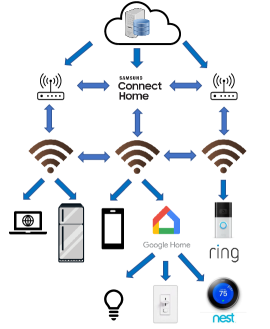
Figure 6: A simplified representation of the smart home system. Our experimental setup contains 23 devices, including 3 WiFi routers, 4 local controllers, 11 sensors/actuators, and over 50 connections.

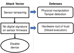
Figure 7: An exploit that employs vulnerabilities in a single device: the Ring garden spotlight camera. The defenses selected by GRAVITAS are shown on the right.

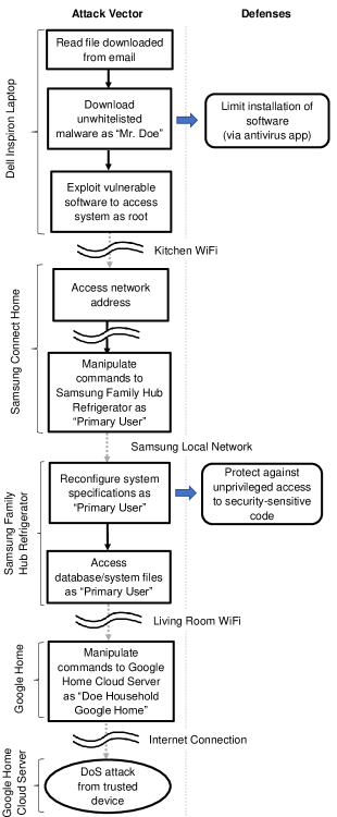
Figure 8: An exploit that employs vulnerabilities in multiple devices. Since there are 17 vulnerabilities in the exploit, not all vulnerabilities (and defenses) in the exploit are shown.

GRAVITAS’s novelty lies in its ability to discover attack vectors (exploit chains) passed over by traditional risk management software. Not only is it effective in discovering attack vectors in a single device (Fig. 7), but it can also discover multi-stage attack vectors that consist of exploiting vulnerabilities in multiple different devices (Fig. 8). These attacks might involve an adversary accessing trusted edge-side devices to gain access to private information in a cloud server, or using illicitly-obtained access to a central controller or user device to disable mission-critical sensing equipment. Both attacks demonstrate GRAVITAS’s ability to include IoT/CPS-specific vulnerabilities in the attack graph, such as physical tampering for edge-side devices. There are numerous paths through the system available to the adversary, and GRAVITAS can find those attack vectors that are most likely to be targeted.

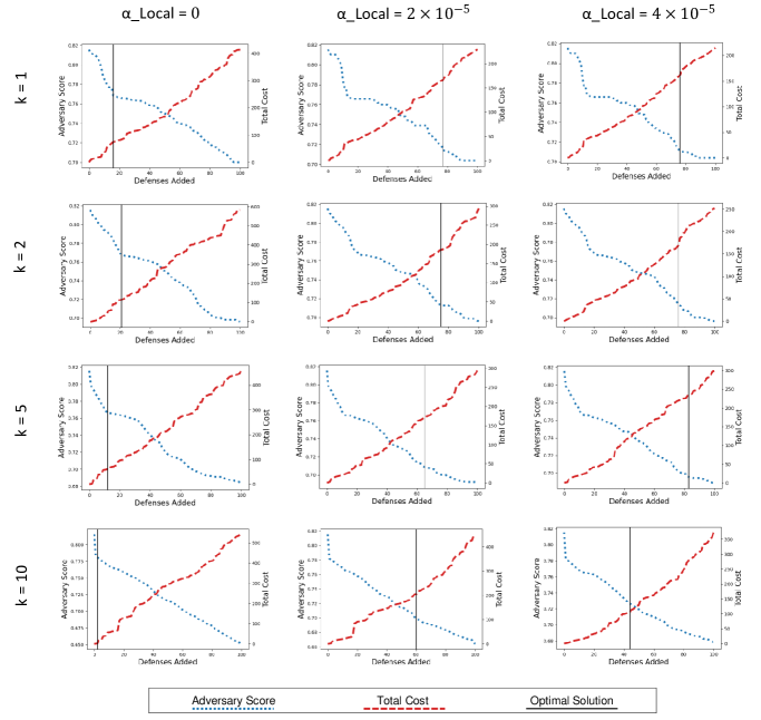
Figure 9: Optimization curves and global optimal solutions during optimization of the smart home system. $\alpha\_Local$ represents the parameter for the local objective function (higher $\alpha\_Local$ means higher cost sensitivity), while $k$ represents the number of entry nodes whose exploit risk scores are averaged to obtain the adversary score. The black line represents the global optimal solution for $\alpha\_Global=0.00032$.

In Fig. 8, we observe that the end result of the exploit is a DoS attack on the cloud server for the Google Home device. Its origin is a malware downloaded onto a laptop, which in turn instructs the Samsung fridge to flood the Google Home server with bogus traffic, thus launching a DoS attack. All this communication occurs via intermediaries such as a Samsung Connect controller and a WiFi router. Although the exploit looks complex, the adversary only needs to know that the laptop user has the Samsung Connect software installed. As a result of the length of this exploit chain, only a select few defenses are necessary to dramatically lower the exploit risk.

The system administrator can view these exploits independently or use GRAVITAS to determine the vulnerabilities that constitute the “weakest link” and disproportionately contribute to the adversary score. Table X shows the three vulnerabilities with the highest exploit risk before defenses are added. Most traditional vulnerability scan-based risk management systems would not mark these vulnerabilities as particularly noteworthy since each cannot significantly compromise the security of its resident device by itself. However, GRAVITAS recognizes the importance of these vulnerabilities due to their crucial role in several attack vectors that lead to attack outcomes with high impact scores. It is worthwhile to also note that these exploit risk scores may be located in vulnerability nodes that are not entry nodes ($n\notin A$); as a result, the entry node exploit risk scores may be lower due to score dilution during the score propagation process.

TABLE X: The smart home vulnerabilities with the highest exploit risk score

Device	Vulnerability	Exploit Risk Score
Ring Base Station	Access requested	0.7190
Ring Front Door Motion Sensor	Sensor tampering	0.7040
Ring Garden Motion Sensor	Sensor tampering	0.7035

This smart home system illustrates how apparently non-fatal vulnerabilities of stand-alone IoT devices can be combined to execute a fatal attack on a multi-device system. One example of this is the “Reconfigure system specifications as primary user” vulnerability of the Samsung Family Hub Refrigerator in Fig. 8. Generally speaking, gaining administrator-level access to an isolated smart fridge would not be a particularly harmful attack. However, because of the fridge’s connection to Google Home and its subsequent connection to the Google Home Cloud Server, that one vulnerability can be used to execute a potent DoS attack via the smart home network hub; this could result in Google blacklisting the hub’s IP address, thus disabling the entire IoT system. This type of attack may not be significant for a small home-based IoT system, but for a Smart Factory, it may have significant economic and safety consequences.

Fig. 9 shows the result of the optimization process using different values of $\alpha\_Local$ (the local objective function weighting parameter) and $k$ (the number of entry node exploit risk scores averaged to obtain the adversary score). These graphs in Fig. 9 show that the adversary score curve generally becomes less “noisy” as $k$ increases. This is expected given that we are averaging more scores for higher $k$. As $\alpha\_Local$ increases, cost is weighted higher in the objective function, and thus the adversary score drops less quickly while the cost also increases less quickly. Changing $k$ or the adversary score has a nonlinear impact on the optimal value (represented by the black line for $\alpha\_Global=0.00032$).

7 Discussion

To enhance the current framework, it may be necessary to occasionally prune the graph and incorporate software-specific vulnerabilities from repositories like the NVD. Tools such as CVE-Search can be used to extract an up-to-date list of vulnerabilities for every device, while off-the-shelf software can be employed to match these vulnerabilities with those in the template attack graphs [25, 39, 29, 40]. Yet even without these additions, GRAVITAS still provides added value in that it considers the whole array of vulnerabilities likely to be present in a device, rather than only those that have already been discovered. This approach allows proactive management of the system, allowing the system administrator to fortify the devices and network connections that would have the highest risk of exploitation if the vulnerability existed.

The categories and subcategories try to encompass the wide range of IoT/CPS devices that exist today, but they cannot realistically be expected to cover all devices. For example, the authentication procedures of embedded devices vary widely, not least because of the dozens of different security protocols and miniature operating systems that these devices use [41]. In addition, the limited graph templates of GRAVITAS may lead the system administrator to “pigeon-hole” their device into an ill-fitting category, accidentally including vulnerabilities that may not exist and excluding those that do exist. Fortunately, GRAVITAS was built to be adaptable: system administrators can easily add additional device templates and known vulnerabilities to the system graphs. As a result, GRAVITAS is adaptable to applications in 5G systems, the design of medical body-area networks, smart city systems, manufacturing facilities, and public utility networks.

The optimization component of GRAVITAS could also be improved. Its “greedy local search” methodology does not consider how adding a defense in the current round will affect the objective function value in later rounds. One possibility is to add “lookahead” functionality that simply adds multiple defenses instead of one to each new entrant in the defense set. A more complex approach would see the local objective function augmented with information about past iterations of the attack graph, perhaps employing a nonlinear estimator for future defense additions.

Despite the cyclic nature of the attack graphs, there were never any convergence issues during the millions of exploit risk score propagation cycles we ran during parameter validation and the smart home tests. Virtually every propagation iteration completed in 50 cycles or less, and none exceeded 100 cycles of propagation. However, there were some issues regarding the consistency of vulnerability scores among different propagation cycles: the exact same graphs with the exact same defenses applied in a different order would sometimes have a slightly different maximum vulnerability score. This is likely due to rounding errors that compound after several thousand floating-point calculations during score propagation. While these errors were immaterial in the Smart Home system and the TASC systems, they do point to the possibility of a “Butterfly Effect” phenomenon in larger systems, where a different random seed or slightly-modified system can have a larger impact on the outcome. To guard against this, the system administrator should perform the entire optimization process multiple times with different seeds so that there are several defense histories from which to pick the optimal solution.

Another issue with GRAVITAS lies in its treatment of defenses. Adding new hardware defenses is difficult post-production, and although it is theoretically possible to add software updates to an existing device, this is not always feasible. For an extant IoT/CPS, rearranging the connections between devices is often far more feasible than changing the devices themselves. Future versions of GRAVITAS should not just be able to add node and edge defenses, but also rearrange the system topology, including permissions and local network connections.

8 Conclusion

GRAVITAS provides new insights into the security of complex IoT/CPS, suggesting new exploits by incorporating potential vulnerabilities into the attack graph and applying strategically-placed defenses that reduce the system’s exploit risk. It is also adaptable to the risk model of the system administrator and can be used to determine which assets are most likely to be impacted in the event of a system breach. GRAVITAS optimizes the defense placements to obtain the best trade-off between system security and cost of operation. Most importantly, GRAVITAS allows for an organization to test and repair the design of an IoT/CPS before deployment, providing a proactive security solution that takes a holistic view of the system. In an era where IoT/CPS will soon be ubiquitous, getting the security right the first time is essential. As a risk assessment tool specifically tailored to the unique devices and complex topology of IoT/CPS, GRAVITAS could become an important tool in the arsenal of security practitioners.

Jacob Brown Jacob Brown received his Bachelor of Science in Electrical Engineering (Hons.) from Princeton University. He has conducted machine learning (ML) research for security and healthcare applications, such as creating a COVID-19 outbreak prediction model based on micro-level demographic data. Jacob has also worked on ML-based geospatial modeling of conflict zones. A member of Sigma Xi, he has received several grants and prizes in recognition of his work, including a grant from the Project X Innovation Fund and the G. David Forney Jr. Prize for an outstanding record in communication sciences.

Tanujay Saha Tanujay Saha is currently pursuing his Ph.D. degree in Electrical and Computer Engineering (ECE) at Princeton University, NJ, USA. He received his Bachelors in Technology (Hons.) from Indian Institute of Technology, Kharagpur, India in 2017. He has held research positions in various organizations and institutes like Intel Corp. (USA), KU Leuven (Belgium), and Indian Statistical Institute. His research interests lie at the intersection of IoT, cybersecurity, machine learning, embedded systems, and cryptography. He has extensive industry and academic experience in both theoretical and practical aspects of cryptography and machine learning.

Niraj K. Jha Niraj K. Jha received the B.Tech. degree in electronics and electrical communication engineering from I.I.T., Kharagpur, India, in 1981, and the Ph.D. degree in electrical engineering from the University of Illinois at Urbana-Champaign, Illinois, in 1985. He has been a faculty member of the Department of Electrical Engineering, Princeton University, since 1987. He was given the Distinguished Alumnus Award by I.I.T., Kharagpur. He has also received the Princeton Graduate Mentoring Award. He has served as the editor-in-chief of the IEEE Transactions on VLSI Systems and as an associate editor of several other journals. He has co-authored five books that are widely used. His research has won 20 best paper awards or nominations. His research interests include smart healthcare, cybersecurity, machine learning, and monolithic 3D IC design. He has given several keynote speeches in the area of nanoelectronic design/test and smart healthcare. He is a fellow of the IEEE and ACM.

References

- [1] A. Mosenia and N. K. Jha, “A comprehensive study of security of Internet-of-Things,” IEEE Trans. Emerging Topics in Computing, vol. 5, no. 4, pp. 586–602, 2017.
- [2] IDC. (2020) Worldwide Spending on the Internet of Things Will Slow in 2020 Then Return to Double-Digit Growth. Report. IDC Corporate USA. [Online]. Available: https://www.idc.com/getdoc.jsp?containerId=prUS46609320
- [3] A. Bosche, D. Crawford, D. Jackson, M. Schallehn, and C. Schorling. (2018) Unlocking opportunities in the Internet of Things. Report. Bain and Company. San Francisco, California. [Online]. Available: https://www.bain.com/contentassets/5aa3a678438846289af59f62e62a3456/bain_brief_unlocking_opportunities_in_the_internet_of_things.pdf
- [4] A. O. Akmandor and N. K. Jha, “Smart health care: An edge-side computing perspective,” IEEE Consumer Electronics Magazine, vol. 7, no. 1, pp. 29–37, 2018.
- [5] B. L. R. Stojkoska and K. V. Trivodaliev, “A review of Internet of Things for smart home: Challenges and solutions,” J. Cleaner Production, vol. 140, pp. 1454–1464, 2017.
- [6] R. Zhang and X. Liu, “IoT-based maintenance process design for fusion reactor remote handling system,” J. Fusion Energy, vol. 33, no. 6, pp. 653–657, 2014.
- [7] M. Yun and B. Yuxin, “Research on the architecture and key technology of Internet of Things (IoT) applied on smart grid,” in Proc. IEEE Int. Conf. Advances in Energy Engineering, 2010, pp. 69–72.
- [8] A. Al-Ali and R. Aburukba, “Role of Internet of Things in the smart grid technology,” J. Computer and Communications, vol. 3, no. 05, p. 229, 2015.
- [9] S. K. Datta, R. P. F. Da Costa, J. Härri, and C. Bonnet, “Integrating connected vehicles in Internet of Things ecosystems: Challenges and solutions,” in Proc. IEEE Int. Symp. A World of Wireless, Mobile and Multimedia Networks, 2016, pp. 1–6.
- [10] A. Thierer and A. Castillo. (2015) Projecting the growth and economic impact of the Internet of Things. Mercatus Center. Arlington, Virginia. [Online]. Available: https://www.mercatus.org/system/files/IoT-EP-v3.pdf
- [11] J. Stavridis and D. Weinstein. (2016, 11) The Internet of Things is a cyberwar nightmare. Foreign Policy Magazine. [Online]. Available: https://foreignpolicy.com/2016/11/03/the-internet-of-things-is-a-cyber-war-nightmare/
- [12] J. A. Lewis. (2016, 2) Managing risk for the Internet of Things. Center for Strategic & International Studies. [Online]. Available: https://csis-website-prod.s3.amazonaws.com/s3fs-public/legacy_files/files/publication/160217_Lewis_ManagingRiskIoT_Web_Redated.pdf
- [13] E. J. Markey and R. Blumenthal. (2020, 6) Letter to acting administrator James Owen concerning cybersecurity issues with Internet-Connected Cars. United States Senate. [Online]. Available: https://www.markey.senate.gov/imo/media/doc/NHTSA%20Cybersecurity%20Followup.pdf
- [14] J. Margolis, T. T. Oh, S. Jadhav, Y. H. Kim, and J. N. Kim, “An in-depth analysis of the Mirai botnet,” in Proc. Int. Conf. Software Security and Assurance, 2017, pp. 6–12.
- [15] V. Sehwag and T. Saha, “TV-PUF: A fast lightweight analog physical unclonable function,” in Proc. IEEE Int. Symp. Nanoelectronic and Information Systems, 2016, pp. 182–186.
- [16] K. McKay, L. Bassham, M. Sönmez Turan, and N. Mouha, “Report on lightweight cryptography,” National Institute of Standards and Technology, Tech. Rep., 2016.
- [17] T. Saha, N. Aaraj, N. Ajjarapu, and N. K. Jha, “SHARKS: Smart hacking approaches for risk scanning in Internet-of-Things and cyber-physical systems based on machine learning,” IEEE Trans. Emerging Topics in Computing, pp. 1–1, 2021.
- [18] A. Mosenia, S. Sur-Kolay, A. Raghunathan, and N. K. Jha, “Physiological information leakage: A new frontier in health information security,” IEEE Trans. Emerging Topics in Computing, vol. 4, no. 3, pp. 321–334, 2016.
- [19] A. Matrosov, E. Rodionov, D. Harley, and J. Malcho. (2011) Stuxnet under the microscope. ESET LLC. [Online]. Available: https://www.esetnod32.ru/company/viruslab/analytics/doc/Stuxnet_Under_the_Microscope.pdf
- [20] G. Hernandez, O. Arias, D. Buentello, and Y. Jin. (2014) A smart Nest thermostat: A spy in your home. Black Hat USA. [Online]. Available: https://www.blackhat.com/docs/us-14/materials/us-14-Jin-Smart-Nest-Thermostat-A-Smart-Spy-In-Your-Home.pdf
- [21] A. Juels, R. L. Rivest, and M. Szydlo, “The blocker tag: Selective blocking of RFID tags for consumer privacy,” in Proc. ACM Conf. Computer and Communications Security, 2003, pp. 103–111.
- [22] L. Huang, A. D. Joseph, B. Nelson, B. I. Rubinstein, and J. D. Tygar, “Adversarial machine learning,” in Proc. ACM Wkshp. Security and Artificial Intelligence, 2011, pp. 43–58.
- [23] IBM Security. (2019) Penetration testing: Protect critical assets using an attacker’s mindset. IBM Corporation. [Online]. Available: https://www.ibm.com/security/services/penetration-testing
- [24] A. Ur-Rehman, I. Gondal, J. Kamruzzuman, and A. Jolfaei, “Vulnerability modelling for hybrid IT systems,” in Proc. IEEE Int. Conf. Industrial Technology, 2019, pp. 1186–1191.
- [25] A. T. Al Ghazo, M. Ibrahim, H. Ren, and R. Kumar, “A2G2V: Automatic attack graph generation and visualization and its applications to computer and SCADA networks,” IEEE Trans. Systems, Man, and Cybernetics: Systems, pp. 1–11, 2019.
- [26] Tenable Inc. (2021) Tenable home page. Tenable Inc. [Online]. Available: https://www.tenable.com/
- [27] X. Ou, S. Govindavajhala, and A. W. Appel, “MulVAL: A logic-based network security analyzer.” in Proc. USENIX Security Symp., vol. 8, 2005, pp. 113–128.
- [28] M. Malowidzki, D. Hermanowski, and P. Berezinkki, “TAG: Topological attack graph analysis tool,” in Proc. Cyber Security in Networking Conf., 2019, pp. 158–160.
- [29] S. Jajodia and S. Noel, Topological Vulnerability Analysis. Center for Secure Information Systems, George Mason University, 2009, pp. 139–154.
- [30] R. Lippmann, K. Ingols, C. Scott, K. Piwowarski, K. Kratkiewicz, M. Artz, and R. Cunningham, “Validating and restoring defense in depth using attack graphs,” in Proc. IEEE Military Communications Conf., 2006, pp. 1–10.
- [31] FIRST. (2019) Common vulnerability scoring system version 3.1 specification document. FIRST Inc. [Online]. Available: https://www.first.org/cvss/v3-1/cvss-v31-specification_r1.pdf
- [32] The European Union Agency for Network and Information Security (ENISA). (2017, 11) Baseline Security Recommendations for IoT in the context of critical information infrastructures. [Online]. Available: https://www.enisa.europa.eu/publications/baseline-security-recommendations-for-iot
- [33] The MITRE Corporation. (2021) MITRE Attack Mitigations - Enterprise. [Online]. Available: https://attack.mitre.org/mitigations/enterprise/
- [34] B. Kordy, L. Piètre-Cambacédès, and P. Schweitzer, “DAG-based attack and defense modeling: Don’t miss the forest for the attack trees,” Computer Science Review, vol. 13-14, pp. 1 – 38, 2014.
- [35] X. Ou and A. Singhal, Quantiative Security Risk Assessment of Enterprise Networks. New York, NY: Springer, 2012.
- [36] S. Noel, L. Wang, A. Singhal, and S. Jajodia, “Measuring security risk of networks using attack graphs,” Int. J. Next Generation Computing, vol. 1, Jan. 2010.
- [37] M. U. Aksu, M. H. Dilek, E. İ. Tatlı, K. Bicakci, H. I. Dirik, M. U. Demirezen, and T. Aykır, “A quantitative CVSS-based cyber security risk assessment methodology for IT systems,” pp. 1–8, 2017.
- [38] FIRST. (2019) Common vulnerability scoring system version 3.1 user guide. FIRST Inc. [Online]. Available: https://www.first.org/cvss/v3-1/cvss-v31-user-guide_r1.pdf
- [39] A. Dulaunoy, P. Moreels, and R. Vinot. (2020) CVE-search project. CVE-Search. [Online]. Available: http://cve-search.org
- [40] OpenVAS - Open Vulnerability Assessment Scanner. Greenbone Networks GmbH. [Online]. Available: https://www.openvas.org/
- [41] O. Hahm, E. Baccelli, H. Petersen, and N. Tsiftes, “Operating systems for low-end devices in the Internet of Things: A survey,” IEEE Internet of Things Journal, vol. 3, no. 5, pp. 720–734, 2016.