Quantum algorithm for the classification of supersymmetric top quark events

Abstract

The search for supersymmetric particles is one of the major goals of the Large Hadron Collider (LHC). Supersymmetric top (stop) searches play a very important role in this respect, but the unprecedented collision rate to be attained at the next high luminosity phase of the LHC poses new challenges for the separation between any new signal and the standard model background. The massive parallelism provided by quantum computing techniques may yield an efficient solution for this problem. In this paper we show a novel application of the zoomed quantum annealing machine learning approach to classify the stop signal versus the background, and implement it in a quantum annealer machine. We show that this approach together with the preprocessing of the data with principal component analysis may yield better results than conventional multivariate approaches.

1 Introduction

After attaining its nominal energy, the Large Hadron Collider (LHC) will reach an unprecedented collision rate during its high luminosity phase, opening the stage to discoveries beyond the standard model (SM) of particle physics. One of the most challenging tasks in searches taking place at the LHC is the capacity to categorize events of new phenomena (signal) and those of SM processes (background) which mimic the signal. Machine learning (ML) tools are among the most powerful means for separating signal from background events, having been key to the discovery of, e.g., the Higgs boson [1, 2]. More recently, quantum annealing for machine learning (QAML) [3] and its zooming variant (QAML-Z) [4] represent the first examples of a quantum approach to a classification problem in high energy physics (HEP).

In this paper, we study the application of the QAML-Z algorithm to the selection of supersymmetric top quark (stop) versus SM events. It is important to test this algorithm on a new classification problem where both the abundance of signal versus background events, and their overlap in the experimental observables are different from [4], therefore allowing us to have a better assessment of its classification capability. A result on the stop search based on the data accumulated by the LHC in 2016 (35.9 fb^-1) has been published [5]. It is based on a classical ML tool which will serve as a reference for gauging the performance of the new classifiers. The variables discriminating between the stop signal and the SM background, which are used to train the QAML-Z algorithm, are based on the same ones as in the classical ML tool [5]. We present results of the QAML-Z algorithm for different schemes of zoomed quantum annealing, and various sets of variables used in the annealer. Also, we introduce a preprocessing of the data through a principal component analysis [6] (PCA) before feeding it to the annealer.

2 Search for supersymmetric top quark

One of the main objectives of the physics program at the LHC are searches for supersymmetry (SUSY) [7, 8, 9, 10, 11, 12], one of the most promising extensions of the SM. SUSY predicts superpartners of SM particles (sparticles) having the same gauge interactions, and whose spin differs by one-half unit with respect to their SM partners. The search for SUSY has special interest in view of the recent discovery of a Higgs boson [1, 2] as it naturally solves the problem of quadratically divergent loop corrections to the Higgs boson mass. In this study we describe the classification aspect of a search for the pair production of the lightest supersymmetric partner of the top quark $\tilde{t}_{1}$ at the LHC machine at $\sqrt{s}$ = 13 TeV, where each stop decays in four objects, see Fig. 1. The lightest neutralino $\tilde{\chi}_{1}^{0}$ is considered to be stable as the lightest supersymmetric particle. The final states considered contain jets, missing transverse energy ($E_{\mathrm{T}}^{\mathrm{miss}}$), and a lepton which can be either a muon or an electron.

Figure 1: Stop pair production at the LHC with four-body decays.

The sensitivity of this type of search is dominated by the capacity to distinguish the stop signal from background events, whose production dominates the signal by several orders of magnitude, and whose observables overlap with the ones of the stop signal. In this search, the main background processes are the $\mathrm{t}\bar{\mathrm{t}}$ and $W+$jets productions. In the search based on a classical ML tool [5], a preselection is first applied to decrease the overwhelming background stemming from the SM. In a second stage, boosted decision trees (BDTs) [13, 14] are used to classify events as signal and background. To find which variables are the most discriminating and should be fed as input to the BDT, different sets of variables are tested as input to a BDT whose output is used to maximize a figure of merit (FOM) [15]:

$$\mathrm{FOM} = \sqrt{2\Big{(}(S+B)\ln\Big{[}\frac{(S+B)\cdot(B+\sigma_{B}^{2})}{B^{2}+(S+B)\cdot\sigma_{B}^{2}}\Big{]}-\frac{B^{2}}{\sigma_{B}^{2}}\ln\Big{[}1+\frac{\sigma_{B}^{2}\cdot S}{B\cdot(B+\sigma_{B}^{2})}\Big{]}\Big{)}},$$ (1)

where $S$ and $B$ respectively stand for the expected signal and background yields for an integrated luminosity of 35.9 fb^-1 at the LHC. The term $\sigma_{B}=(f\cdot B)$ represents the expected systematic uncertainty on the background with $f$ being the relative uncertainty of the background yield, taken to be $f=20\%$ as in [5]. The set of variables which maximize the FOM is chosen as the final set of input variables to the BDT. This metric captures the full information of the statistical and systematic uncertainties of a given selection, as it is important to account for the actual conditions of a search. The approach based on the maximization of this FOM has been very effective to find the smallest and most efficient set of discriminating variables in several searches [5, 16]. A description of the BDT parameters as well as its development with a FOM maximization procedure as used in [5] are provided in Appendix A. The list of variables is presented in Table 1 and their distribution for signal and background is provided in Fig. 2. To render the results of the classification based on the QAML-Z algorithm as comparable as possible to the one of [5], we use the same preselection of events before training (see Appendix A). Furthermore, since the FOM as defined in Eq. 1 represents a complete and single-number measure of the power of a selection, we evaluate the performance of the QAML-Z algorithm by a maximization of the FOM versus a cut on its output. Finally, for the comparison of performances to reflect only the difference of a quantum based versus a classical tool, we train the QAML-Z algorithm with different sets made of the same discriminating variables as in the BDT based search [5] (see Table 1).

Variable	Description
$p_{\mathrm{T}}(l)$	$p_{\mathrm{T}}$ of the lepton $l$
$\eta(l)$	Pseudorapidity of the lepton $l$
$Q(l)$	Charge of the lepton $l$
$E_{\mathrm{T}}^{\mathrm{miss}}$	Missing transverse energy
$M_{\mathrm{T}}$	Transverse invariant mass of
	the ($E_{\mathrm{T}}^{\mathrm{miss}}$,$p_{\mathrm{T}}(l)$) system
$N(\mathrm{jets})$	Multiplicity of selected jets
$p_{\mathrm{T}}(j_{1})$	$p_{\mathrm{T}}$ of the leading jet
$H_{\mathrm{T}}$	$\sum_{i}p_{\mathrm{T}}(jet(i))$
$\mathrm{Disc(b)}$	Maximum b-quark tagging discriminant of the jets
$N(b)$	Number of b-tagged jets
$p_{\mathrm{T}}(b)$	$p_{\mathrm{T}}$ of the jet with the highest
	b-discriminant
$\Delta R(l,b)$	Distance between the lepton and the
	jet with the highest b-discriminant

Table 1: List of discriminating variables used as input to a BDT in [5].

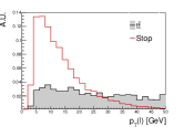
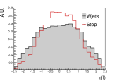
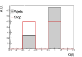
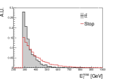
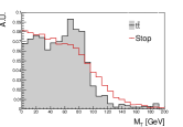
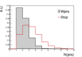
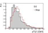
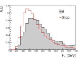
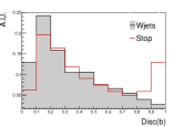
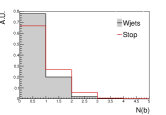
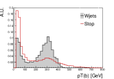
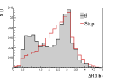
Figure 2: Distribution of the discriminating variables for the stop signal with $\Delta m=30$, $W+$jets and $\mathrm{t}\bar{\mathrm{t}}$ , used as input to a BDT in [5]. From top-left to bottom-right: $p_{\mathrm{T}}(l)$, $\eta(l)$ , $Q(l)$ , $E_{\mathrm{T}}^{\mathrm{miss}}$, $M_{\mathrm{T}}$, $N(\mathrm{jets})$ , $p_{\mathrm{T}}(j_{1})$ , $H_{\mathrm{T}}$, $\mathrm{Disc(b)}$ , $N(b)$ , $p_{\mathrm{T}}(b)$ , $\Delta R(l,b)$ . Distributions are normalized to the same area and shown at preselection.

3 Quantum annealing and zooming

From the distribution of each variable $i$ in signal and background events, we construct a weak classifier $\chi_{i}$ as in [3] which retains the discriminant character of each variable while adapting it to an annealing process. We then construct an Ising problem as follows. For each training event $\tau\in[1,S]$, we consider the vector $x_{\tau}$ of the values of each variable of index $i$ we use, and a binary tag $y_{\tau}$ labeling the event $\tau$ as either signal ($+1$) or background ($-1$). The value of the $i$th weak classifier for the event $\tau$ is given by the sign of the corresponding weak classifier $\chi_{i}$: $c_{i}(x_{\tau})=\mathrm{sgn}(\chi_{i}(x_{\tau}))/N=\pm 1/N$, where $N$ is the number of weak classifiers. In the QAML algorithm, the optimization of the signal-background classification problem is expressed in terms of the search for the set of spins $s_{i}$ minimizing the Ising Hamiltonian:

$$H_{\mathrm{Ising}} = \sum\limits_{i=1}^{N}h_{i}s_{i}+\sum\limits_{i=1}^{N}\sum\limits_{j>i}^{N}J_{ij}s_{i}s_{j}$$ (2)

$$= \sum\limits_{i=1}^{N}\Big{(}\lambda-C_{i}+\frac{1}{2}\sum\limits_{j>i}^{N}C_{ij}\Big{)}s_{i}+\frac{1}{4}\sum\limits_{i=1}^{N}\sum\limits_{j>i}^{N}C_{ij}s_{i}s_{j}$$

where $h_{i}$ is the local field on spin $s_{i}$, and $J_{ij}$ is the coupling between spins $s_{i}$ and $s_{j}$. The factor $\lambda$ is a regularization constant, and the terms $C_{i}$ and $C_{ij}$ are defined as function of weak classifier values and event tags as:

$$C_{i}=\sum\limits_{\tau=1}^{S}c_{i}(x_{\tau})y_{\tau}, C_{ij}=\sum\limits_{\tau=1}^{S}c_{i}(x_{\tau})c_{j}(x_{\tau}).$$ (3)

A strong classifier $R$ is then built as a linear combination of all weak classifiers and the spins, merging for each event the discriminating power provided by all $c_{i}$’s and the spins $s_{i}$ obtained from the quantum annealing process. The minimization of the classification error is performed by the minimization of the Euclidean distance between the binary tag of each event and its classification $R$ as obtained by the annealing:

$$||y-R||^{2} = \sum\limits_{\tau=1}^{S}|y_{\tau}-\sum\limits_{i=1}^{N}s_{i}c_{i}(x_{\tau})|^{2}.$$ (4)

In the QAML-Z approach, the quantum annealing is operated iteratively while a substitution is made to the spin $s_{i}$:

$$s_{i} \longrightarrow \mu_{i}(t)+s_{i}\cdot\sigma(t)=\mu_{i}(t+1),$$ (5)

where:

• $\mu_{i}(t)$ is the mean value of qubit $i$ at time $t$. We have: $\forall i$ $\mu_{i}(0)=0$.

• $\sigma(t)$ is the search width at each annealing iteration $t$. We have: $\sigma(t)=b^{t}$ where $b=\frac{1}{2}$ and $t\in[0,T-1]$.

This iterative procedure effectively shifts and narrows the region of search in the space of spins. It updates the vector $\mu_{i}$ which is collected at the final iteration to form the strong classifier:

$$R(x_{\tau}) = \sum\limits_{i=1}^{N}\mu_{i}(T-1)c_{i}(x_{\tau}),$$ (6)

where the use of the weak classifiers is not limited to the binary choice $\{0,1\}$, but is extended to the continuous interval $[-1,1]$ via the use of the vector $\mu_{i}$. The classification capacity of the QAML-Z algorithm is further enhanced by an augmentation scheme applied on the weak classifiers. For each $h_{i}$, several new classifiers $c_{il}$ are created:

$$c_{il}(x_{\tau}) = \frac{\mathrm{sgn}(h_{i}(x_{\tau})+\delta l)}{N},$$ (7)

where $l\in\mathbb{Z}$ is the offset: $-A\leq l\leq A$, and $\delta$ is the step size. While the value $c_{i}$ of the old classifier has only a binary outcome for each $h_{i}$, the new classifiers $c_{il}$ have similar but $(2A+1)$ different outcomes depending on the very distribution of $h_{i}$. We therefore have a better discrimination because a more continuous, thus more precise representation of the spectrum of $h_{i}$ with $c_{il}$ than with $c_{i}$. Applying the substitution of Eq. 5 in Eq. 4, omitting spin independent and quadratic self-spin interaction terms, and defining new indices $I$ as $\{il\}$ and $J$ as $\{jl^{\prime}\}$, we obtain the Hamiltonian (see Appendix B):

$$H(t)=\sum_{I=1}^{N(2A+1)}\left(-C_{I}+\sum_{J=1}^{N(2A+1)}\mu_{J}(t)C_{IJ}\right)\sigma(t)s_{I}+\frac{1}{2}\sum_{I=1}^{N(2A+1)}\sum_{J\neq I}^{N(2A+1)}C_{IJ}\sigma^{2}(t)s_{I}s_{J},$$ (8)

with:

$$C_{I}=\sum\limits_{\tau=1}^{S}c_{il}(x_{\tau})y_{\tau}, C_{IJ}=\sum\limits_{\tau=1}^{S}c_{il}(x_{\tau})c_{jl^{\prime}}(x_{\tau}).$$ (9)

The terms $C_{I}$ and $C_{IJ}$ are the input to the classification problem. The Hamiltonian $H(t)$ is iteratively optimized for $t$, with the vector $\mu_{I}$ updated similarly to Eq. 5. The information about the iterative quantum annealing, corresponding parameters, and control results are provided in Appendix C, where we ensure that the Ising model energy decreases and stabilizes for the chosen parameters. The output of the optimization procedure is a strong classifier built as in Eq. 6, and whose distribution is used to discriminate signal from background.

4 Classification of stop with the QAML-Z algorithm

As in [5], only the main background processes $W+$jets and $\mathrm{t}\bar{\mathrm{t}}$ are used for training the QAML-Z algorithm. To realistically represent the SM in the training, a background sample is formed where events of these two processes are present proportionally to their production rate at the LHC. We divide this sample in two equal parts, one being used by the QAML-Z algorithm and one to assess the performance of the strong classifier through the maximization of the FOM: N(Sample)=N($QA$)+N(Assess). The $QA$ sample is further divided in two equal parts, one to train the annealer and another one to test for over-training in the annealer: N($QA$)=N(Train)+N(Test). It should be noted that only the Train sample is involved in the annealing process. Having shown [5] that the kinematic properties of all signal points $(m(\tilde{t}_{1}),m(\tilde{\chi}_{1}^{0}))$ are quasi identical along the line $\Delta m=m(\tilde{t}_{1})-m(\tilde{\chi}_{1}^{0})$, we use all signal events with $\Delta m=30$ except the signal point $(550,520)$ as $QA$ sample, while entirely using this latter signal as Assess sample. This organization of samples allows the usage of a maximal number of both signal and background events for assessing the performance of the classification as well as testing the annealing process.

The data is run on the $2000Q$ quantum annealer of D-Wave Systems Inc. [17], where the time to solution is $O(\mu s)$, ie. the time of the annealing (see Appendix C). This computer is based on the Chimera graph which has 2048 qubits and 5600 couplers. To embed the Ising Hamiltonian in the annealer, qubits of the graph are ferromagnetically coupled into a chain to represent a single spin of the Hamiltonian $H(t)$. While the Hamiltonian in Eq. 8 is fully connected, the Chimera graph is not, thus limiting the hardware implementation of the classification problem. The number of $J_{ij}$ couplers is given by: $N(J_{ij})=N_{\mathrm{v}}\cdot(N_{\mathrm{v}}-1)/2$ with $N_{\mathrm{v}}=N_{\mathrm{var}}\cdot(2A+1)$, where $N_{\mathrm{var}}$ is the number of variables used to train the QAML-Z algorithm, and $A$ is a parameter of the augmentation scheme (see Eq. 7). Given the number of variables and the augmentation schemes used, the limit of 5600 couplers can be exceeded by $N(J_{ij})$; typically, for $N_{\mathrm{v}}$=12 and for an augmentation with $A$=5, the needed number of couplers is 8646. We therefore prune the elements of the $J_{ij}$ matrix, retaining the largest $(1-C)$ elements, where $C$ is a cutoff percentage. Different cutoff values are expected to optimize the performance for different sets of variables and different augmentations schemes ($A,\delta$). As a further option to reduce the size of the Ising model to be encoded on the annealer, we use the polynomial-time variable fixing scheme of the D-Wave API. This scheme is a classical procedure to fix the value of a portion of the input variables to values that have a high probability of being optimal. An illustration of the effect of the cutoff $C$, the use of variable fixing, and the augmentation scheme is given in Appendix C.

In order to compare the performance of a quantum annealing with a classical ML counterpart, we explore various $settings$ of the QAML-Z algorithm, namely different augmentation schemes, cutoffs, and variable fixing options, reporting only the performance of the best setting for each tested set of variables (see Sec. 5). Despite averaging out the random errors on the annealing and mitigating the possible effects of overfitting due to zooming (see Sec. 3), the outcome of the annealing (the vector $\mu_{I}$) can vary due to the probabilistic nature of these schemes and to the variations of the machine itself (e.g. low-frequency flux noise of the qubits), leading to an uncertainty on the performance. In order to estimate this uncertainty, we run the annealing ten times with the same input variables, in the very same setting, and on the same sample of events, and we consider the standard deviation of the corresponding maximal FOMs as uncertainty of the performance for a given set of variables and setting. In Fig. 3 we report the performance of the QAML-Z algorithm with the variables of Table 1 as input and with a given augmentation scheme and cutoff as a function of the number of events used in the training. The performance of the annealer increases with N(Train), witnessing a clear rise for rather small number of events and a more moderate increase for larger numbers of events, confirming the results of [3] with another signal. Henceforth, we will present all results for N(Train)=N(Test)=50$\cdot$10³ where signal and background events respectively represent 40% and 60% of these two samples. We therefore benefit from a large sample size to train the QAML-Z algorithm, while observing a quasi identical evolution of the Hamiltonian energy for the Train and Test samples (see Fig. 5 in Appendix C). The Assess sample contains approximately 200$\cdot$10³ background, and 7$\cdot$10³ signal events. In Fig. 4 we present the distribution of the strong classifier for signal, and the two main background processes. As can be observed, there is no over-training of the QAML-Z algorithm because the response of the strong classifier is statistically very similar for events which are used to train the annealer and those not exposed to the training. Also shown in Fig. 4 is the evolution of the FOM in the Assess sample as function of the cut applied on the output of the strong classifier. Henceforth, all the reported values of maximal FOM are checked to correspond to a cut where there are enough events in both signal and background samples.

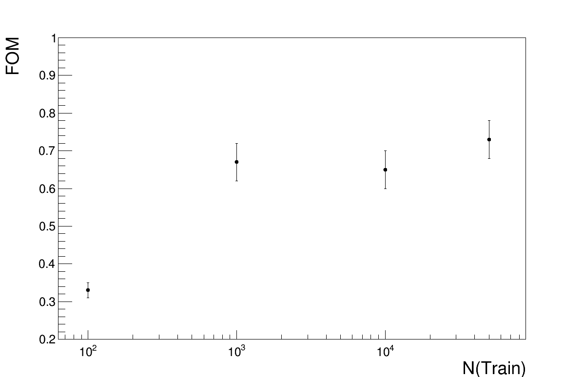
Figure 3: Evolution of the FOM as a function of the number events used for training. The QAML-Z algorithm uses the variables of Table 1 transformed in weak classifiers, with an augmentation scheme of ($\delta$,$A$)=(0.025,3), and with a cutoff $C$=85%, without using a variable-fixing procedure.

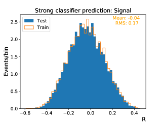
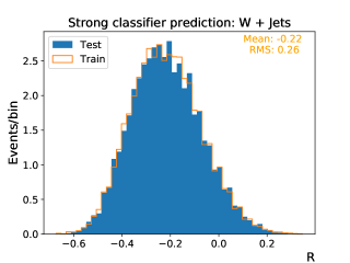
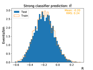
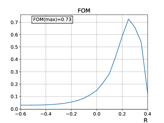
Figure 4: The output of the strong classifier for the signal (top-left), $W+$jets (top-right) and $\mathrm{t}\bar{\mathrm{t}}$ background (bottom-left) in the train (orange) and test (blue) events within the $QA$ sample. The evolution of the FOM as a function of the cut applied on the strong classifier’s output is illustrated in the plot in the bottom-right. The QAML-Z algorithm uses the variables of Table 1 transformed in weak classifiers, with an augmentation scheme of ($\delta$,$A$)=(0.025,3), and with a cutoff $C$=85%, without using a variable-fixing procedure. The number of events used for training is N(Train)=50$\cdot$10³.

5 Approaches and results

We define the main sets of tested variables in Table 2. For each set and the different approaches to test it, we perform an extensive study of the performance of the QAML-Z algorithm for different augmentation schemes, cutoffs, and the use (or not) of variable fixing, as illustrated for the sets A and B respectively in Fig. 6 and 7 of Appendix C. For each set and approach, we report the optimal setting and the corresponding performance in Table 3.

The set $\alpha$ contains the variables defined in Table 1 where the discriminating variables are not transformed into weak classifiers, being only normalized to the [$-1$,$+1$] interval. The set $\beta$ consists of the same variables where these are transformed into weak classifiers. As can be seen in Table 3, the performance of the set $\beta$ is expectedly higher than for the set $\alpha$, where the weak classifiers are scaled as a function of the initial distribution of the discriminating variables to better reflect the separation between signal and background. The transformation into weak classifiers is performed for all subsequent tests.

We explore in a second step the effect of additional discriminating variables built from the same initial set of Table 1. The methodology followed to built these new variables in explained in Appendix D, where the discriminating power of each variable is appraised via its maximal FOM. Two new sets of variables are constructed based on these new variables, as reported in Table 2: the set A including the variables of the Table 1 and new variables with the highest FOMs, and the set B including those of set A and additional variables with the lower FOMs (see Table 4). As can be observed in Table 3, the addition of variables with higher maximal FOMs in the set A increases the performance of the QAML-Z algorithm, while the further addition of variables with lower FOM in the set B does not significantly improve the quality of the classification.

The results of the search [5] are based on the use of BDT where the discriminating variables are diagonalized before being fed to the training [13, 14]. This step better prepares the data for classification because the original discriminating variables do not necessarily constitute the optimal basis in which signal and background are optimally separated. In order to render our approach as comparable as possible to the one followed with a BDT [5], we pass our data through the procedure of PCA [6] before feeding it to the QAML-Z algorithm. It must be noted that the use of PCA is only one method for diagonalizing the data, other methods also being applicable to this end. The application of PCA on the data before the quantum annealing further improves the results for the set of variables A, and to a lesser extent for B, as can be seen in Table 3. We note a larger uncertainty of the QAML-Z algorithm where the data is prepared with the PCA, this for the same sets of variables. In the PCA basis, the weak classifiers are more decorrelated from each other, rendering the corresponding weights $\mu_{I}$ more independent from one another. When a $\mu_{I}$ fluctuates (e.g. because of the state of the machine), the strong classifier $R$ (see Eq. 6) is sensitive to the variations of a larger number of $\mu_{I}$’s, hence a larger variation of its outcome. It is noticeable that the QAML-Z algorithm, once put on a footing as similar as possible to the BDT based approach [5], can reach an equivalent, possibly better performance. It is interesting to observe that the best result is achieved without using the variable fixing scheme, where the annealing is put at full use.

Variable	List of	Use of weak
set name	variables	classifiers
$\alpha$ / $\beta$	Table 1	No / Yes
A	Table 1 and:	Yes
	$p_{\mathrm{T}}(l)$/$E_{\mathrm{T}}^{\mathrm{miss}}$, $p_{\mathrm{T}}(l)$/$p_{\mathrm{T}}(j_{1})$ ,
	($\mathrm{Disc(b)}$ $-$1)$p_{\mathrm{T}}(b)$ ,
	$|$($E_{\mathrm{T}}^{\mathrm{miss}}$$-$280)($M_{\mathrm{T}}$$-$80)$|$ ,
	$|$($E_{\mathrm{T}}^{\mathrm{miss}}$$-$280)($H_{\mathrm{T}}$$-$400)$|$
B	Variables of set A and:	Yes
	$\Delta R(l,b)$ $-$ ($M_{\mathrm{T}}$/40) ,
	$H_{\mathrm{T}}$2/$N(\mathrm{jets})$ , $p_{\mathrm{T}}$  $+$ 3.5$\eta(l)^{2}$ ,
	$p_{\mathrm{T}}$ /$H_{\mathrm{T}}$

Table 2: Definition of different variable sets as a function of the used variables.

Variable	Fixing	$C$ [%]	($\delta$,$A$)	FOM
set	variable
$\alpha$	False	85	(2.50$\cdot$10-2,3)	0.48 $\pm$ 0.03
$\beta$	False	85	(2.50$\cdot$10-2,3)	0.73 $\pm$ 0.03
A	True	95	(0.90$\cdot$10-2,5)	0.88 $\pm$ 0.04
B	True	85	(0.70$\cdot$10-2,3)	0.91 $\pm$ 0.05
PCA(A)	False	95	(1.45$\cdot$10-2,3)	1.57 $\pm$ 0.24
PCA(B)	True	95	(0.70$\cdot$10-2,5)	1.09 $\pm$ 0.17
BDT	NA	NA	NA	1.44 $\pm$ 0.06

Table 3: Best performance obtained for different sets of variables as defined in Table 2, and for different approaches applied on some sets. The corresponding use (or not) of variable fixing, cutoff and augmentation scheme are reported. All results are provided for N(Train)=50000. For comparison, the performance of the BDT of [5] is also reported, where “NA” stands for nonapplicable.

6 Summary

We studied the capability of the quantum annealing, where the zoomed and augmented QAML-Z approach is applied to a new classification problem, namely the discrimination of stop versus SM background events. The classification is based on well motivated variables whose discriminating power has been tested with a FOM maximization procedure. The use of this latter metric constitutes a novel and reliable assessment of the performance of a selection as it includes its full statistical and systematic uncertainties. We systematically tested each set of variables used by the QAML-Z algorithm for different augmentation schemes and percentages of pruning on the couplers of the annealer as to find the optimal setting. The performance of different settings is assessed for large training samples which are observed to yield the best performances, and are also more adapted to the needs of experimental particle physics where very large data samples are used. We observe an improvement of the classification performance when adding variables with a high FOM. To put the annealing approach and the classical BDT approach on the same footing, we pass the data through a PCA procedure before feeding it to the quantum annealer. For the first time in HEP, we show that for large training samples the QAML-Z approach running on the Chimera graph reaches a performance which is at least comparable to the best-known classical ML tool. With more recent graphs there is the prospect that the larger number of connected qubits will yield a better correspondence between the Ising Hamiltonian and the system of qubits of the annealer. The larger number of available couplers in the machine will allow a more complete use of the information contained in the couplers of the Hamiltonian; it will render each chain more stable, thus less prone to be broken, where the discriminating information of the classification will be more effectively used.

Appendix A Samples and signal selection

The data used for training and testing the QAML-Z algorithm are events simulating proton-proton collisions of the LHC at $\sqrt{s}$ = 13 TeV. The generation of the signal and background processes is performed with the Madgraph52.3.3 [18] generator. All samples are then passed to Pythia 8.212 [19, 20] for hadronization and showering. The detector response is simulated with the Delphes.3 [21] framework.

The first step in the search is the preselection, which is common to the search [5] and to the present study. We require $E_{\mathrm{T}}^{\mathrm{miss}}$$>280$ GeV to select preferentially signal, as the production of two $\tilde{\chi}_{1}^{0}$ escaping detection increases the missing transverse energy in the detector. The leading jet of each event is required to fulfill $p_{\mathrm{T}}$ $>110$ GeV and $|\eta|<2.4$. A cut of $H_{\mathrm{T}}$$>200$ GeV is imposed. This cut diminishes the contribution of the $W+$jets background where jets are softer than for signal. At least one identified muon (electron) with $p_{\mathrm{T}}$ $>3.5$ $(5)$ GeV and $|\eta|<2.4$ ($2.5$) must be present. Events with additional leptons with $p_{\mathrm{T}}$ $>$ 20 GeV are rejected, diminishing the contribution of the $\mathrm{t}\bar{\mathrm{t}}$ background with two leptons. Background from SM dijet and multijet production are suppressed by requiring the azimuthal angle between the momentum vectors of the two leading jets to be smaller than 2.5 rad for all events with a second hard jet of $p_{\mathrm{T}}$ $>60$ GeV.

The second step in the selection of the signal is the usage of an approach more advanced than linear cuts. We describe here the parameters of the BDT as used in [5], and the procedure to include different discriminating variables as its inputs. We define $N_{T}$ and $M_{D}$ respectively as the number of trees in the BDT and its maximal depth. The maximal node size $M_{N}$ is the percentage of the number of signal or background events at which the splitting of data stops in the tree, and acts as a stopping condition of the training. These parameters are optimized by maximizing the FOM of different BDTs trained with various parameters. The setting yielding the best performance while avoiding an over-training is ($N_{T}$, $M_{D}$, $M_{N}$)=(400, 3, 2.5%). Finally, the space of input variables is diagonalized before being fed to the training. As for the procedure to include discriminating variables as inputs to the BDT, we start from a reduced set $\xi$ which comprises the basic variables of the search. A new variable $v$ is incorporated into the set of input variables only if it significantly increases the FOM. Namely, we train a BDT with the set $\xi$ and another with $\xi\oplus v$, and calculate the FOM of Eq. 1 as a function of the cut applied on the BDT’s output. If the maximal FOM reached with the latter set is higher than the one with the former, the variable $v$ is incorporated as a new input variable; if the performance of the set $\xi\oplus v$ is compatible with the one of $\xi$, it is not. This procedure is repeated until there is no new variable at disposal.

In order to make the comparison with the results of quantum annealing as valid as possible, a BDT is re-trained with the Delphes simulation. The performance, for the same signal, is compatible between this new simulation and the full simulation of the CMS detector.

Appendix B Derivation of the Hamiltonian

In this section, we derive the expression of the Hamiltonian to be iteratively minimized, first for the zooming and then for the augmentation step. If we expand the Euclidean distance of Eq. 4 to be minimized, we obtain:

$$\sum_{\tau=1}^{S}\left[||y_{\tau}||^{2}+\left(\sum_{i=1}^{N}s_{i}c_{i}\left(\textbf{x}_{\tau}\right)\right)^{2}-2y_{\tau}\left(\sum_{i=1}^{N}s_{i}c_{i}\left(\textbf{x}_{\tau}\right)\right)\right].$$ (10)

Omitting the first term which is constant, and inserting the zooming substitution of Eq. 5 in Eq. 10, we obtain:

$$\sum_{\tau=1}^{S}\left[\left(\sum_{i=1}^{N}(\sigma(t)s_{i}+\mu_{i}(t))c_{i}(\textbf{x}_{\tau})\right)^{2}-2y_{\tau}\left(\sum_{i=1}^{N}(\sigma(t)s_{i}+\mu_{i}(t))c_{i}(\textbf{x}_{\tau})\right)\right].$$ (11)

Fully developing the Eq. 11 while neglecting constant, spin independent, and quadratic self-spin interaction terms, we get:

$$\sum_{\tau=1}^{S}\left[-2y_{\tau}\sum_{i=1}^{N}\sigma(t)c_{i}(\textbf{x}_{\tau})s_{i}+2\sum_{i=1}^{N}\left(\sum_{j=1}^{N}\mu_{j}(t)c_{j}(\textbf{x}_{\tau})\right)\sigma(t)c_{i}(\textbf{x}_{\tau})s_{i}+2\sum_{i=1}^{N}\sum_{j>i}^{N}(\sigma^{2}(t)c_{i}(\textbf{x}_{\tau})c_{j}(\textbf{x}_{\tau}))s_{i}s_{j}\right].$$ (12)

Recalling the definition of the terms $C_{i}$ and $C_{ij}$ in Eq. 3, and dividing the expression 12 by two, we obtain the expression of the Hamiltonian with the zooming approach:

$$H(t) = \sum\limits_{i=1}^{N}\Big{(}-C_{i}+\sum\limits_{j=1}^{N}\mu_{j}(t)C_{ij}\Big{)}\sigma(t)s_{i}+\sum\limits_{i=1}^{N}\sum\limits_{j>i}^{N}C_{ij}\sigma^{2}(t)s_{i}s_{j}.$$ (13)

Now we augment each classifier $i$ with $(2A+1)$ classifiers:

$$\forall i,\exists l / c_{i}\longrightarrow c_{il},$$ (14)

where $l\in\mathbb{Z}$ is the offset: $-A\leq l\leq A$, as defined in Eq. 7. Inserting the augmentation substitution 14 in Eq. 13 and omitting constant terms, we obtain:

$$H(t)=\sum_{l=-A}^{+A}\sum_{i=1}^{N}\left(-\sum_{\tau=1}^{S}c_{il}y_{\tau}+\sum_{l^{\prime}=-A}^{+A}\sum_{j=1}^{N}\mu_{jl^{\prime}}(t)\sum_{\tau=1}^{S}c_{il}c_{jl^{\prime}}\right)\sigma(t)s_{il}+\frac{1}{2}\sum_{l=-A}^{+A}\sum_{i=1}^{N}\sum_{\{j,l^{\prime}\}\neq\{i,l\}}\sum_{\tau=1}^{S}c_{il}c_{jl^{\prime}}\sigma^{2}(t)s_{il}s_{jl^{\prime}}.$$ (15)

Using the equivalence:

$$\forall X, \sum\limits_{i=1}^{N}\sum\limits_{l=-A}^{A}X_{il} \equiv\sum\limits_{I=1}^{N(2A+1)}X_{I},$$ (16)

and defining the new indices $I$ and $J$ as $\{il\}$ and $\{jl^{\prime}\}$ respectively, we obtain the expression of the final Hamiltonian which includes the zooming and augmentation approaches:

$$H(t)=\sum_{I=1}^{N(2A+1)}\left(-C_{I}+\sum_{J=1}^{N(2A+1)}\mu_{J}(t)C_{IJ}\right)\sigma(t)s_{I}+\frac{1}{2}\sum_{I=1}^{N(2A+1)}\sum_{J\neq I}^{N(2A+1)}C_{IJ}\sigma^{2}(t)s_{I}s_{J},$$ (17)

with:

$$C_{I}=\sum\limits_{\tau=1}^{S}c_{il}(x_{\tau})y_{\tau}, C_{IJ}=\sum\limits_{\tau=1}^{S}c_{il}(x_{\tau})c_{jl^{\prime}}(x_{\tau}).$$ (18)

It has to be noted that the Hamiltonians of both equations 13 and 17 are fully connected.

Appendix C Quantum annealing: parameters and control results

During the iterative optimization of the Hamiltonian, and to average out random errors on the local fields and couplings, each annealing is run and averaged over $n_{g}$ gauges [22] and $n_{e}$ maximal number of excited states, where $n_{g}$ and $n_{e}$ can be made to monotonically decrease with each iteration. To mitigate the impact of overfitting due to the zooming, we follow a two-step randomization procedure in each iteration: if the energy of the qubit $i$ worsens, a sign flip $s_{i}\rightarrow-s_{i}$ is applied with a monotonically decreasing probability $p_{f}(t)$, followed by a randomly uniform spin flip for all qubits with probability: $q_{f}(t)<p_{f}(t)$ $\forall t$; the values of the two probabilities per iteration are kept the same as in [4]. Building on the results of [3, 4], we set the number of iterations to 8, while setting the annealing time to 20 $\mu s$. During this iterative optimization, the annealing is run for $n_{g}$ gauges at each iteration to reduce random errors on the local fields $h_{i}$ and couplers $J_{ij}$. For each gauge, the annealing result is sampled 200 times, and the set of spins leading to the lowest energy is collected. The selection of the excited states is based on a distance $d$ to the state of lowest energy and a maximal number $n_{e}$ of excited states as in  [4], where the value of $n_{g}$, $n_{e}$ and $d$ varies with the iteration. This means that after the iteration $t$ we have a set of $n_{g}(t)$ different $\mu_{I}$’s, out of which at most $n_{e}(t)$ are kept for the next iteration, corresponding to the best energies. At iteration $t+1$, we have at most $n_{e}(t)\cdot n_{g}(t)$ annealings, thus states, out of which at most $n_{e}(t+1)$ are kept. This represents a lot of computing time. For the problem optimized in this paper, and for a given set of variables, we compared results obtained with $n_{g}=\{50,10,1,...,1\}$ and $n_{e}=\{16,4,1,...,1\}$ as in [4] on one hand, with results obtained with $n_{g}=\{50,10,...,10\}$ and $n_{e}=\{1,...,1\}$ on the other. We observed that the obtained energies were quasi-identical for a large number of training events, showing that picking the state of best energy out of $n_{g}>1$ is sufficient to mitigate the uncertainties of the annealing process, while saving computing time. We therefore retain the latter options for $n_{g}$ and $n_{e}$. Finally, the chain strength $r$ is defined as the ratio of the coupling within each chain over the largest coupling in Hamiltonian. If $r$ is very large, the chains will be too strong to allow a multiqubit flipping which is necessary to explore the space of spins. If on the contrary $r$ is very small, the chains will be broken by the tension induced by the problem or by thermal excitation. The chain strength can be set to decay monotonically with each iteration as to allow $H(t)$ to drive the system dynamics while preventing the chains of qubits from breaking [23]. The value of $r$ at each iteration is the same as in [4]. In the case where the chain is broken, the measure of the qubit chains is performed through a majority vote, possibly leading to the collection of non-optimal sets of solution spins, thus to a possible loss of discriminating information.

In Fig. 5 we present the evolution of the Ising Hamiltonian energy as a function of the optimization iteration for different numbers of events used to train the QAML-Z algorithm. One can observe that the energy decreases with the iteration, and that the difference of energy between events used to train and test the annealer decreases for higher N(Train). In figures 6 and 7 we report the performance of the QAML-Z algorithm for variable sets A and B as defined in Table 2, and for different augmentation schemes, cutoffs $C$ and variable-fixing options. Lower values of $C$ than those illustrated in these figures are not reported because no embedding was found given the number of variables and tested augmentation scheme. It is interesting to note that the lowest bound for $C$ is higher for the set B where the number of variables is higher, and for a higher augmentation range (variable $A$) which leads to a larger number of $c_{il}$ (see Eq. 7), thus coupling terms $C_{IJ}$ (see Eq. 9). Depending on the set of variables and the augmentation scheme, different values of $C$ are optimal. The performance is generally higher when the variable-fixing procedure is used. For a given set of variables, small or big values of the offset $\delta$ (see Eq. 7) might lead to a disadvantageous augmentation of the weak classifiers, leading to non-optimal performance. This is illustrated for the performances of the set B in Fig. 7 where the FOM raises then drops for decreasing values of $\delta$, this for almost all values of cutoff.

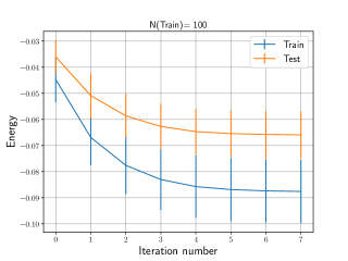
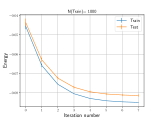
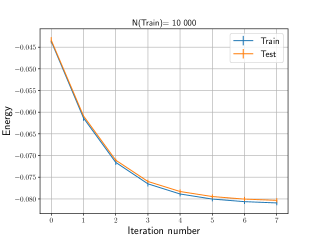
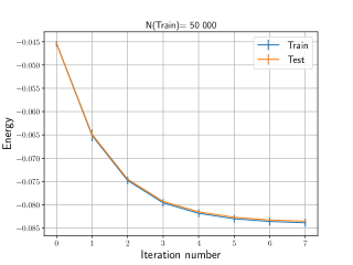
Figure 5: Evolution of the Ising Hamiltonian energy as a function of the iteration for N(Train) varying from 100 (top left) to 50000 (bottom right), these in the train (blue) and test (orange) samples. The QAML-Z algorithm uses the variables of Table 1 transformed in weak classifiers, with an augmentation scheme of ($\delta$,$A$)=(0.025,3) and a cutoff of 85%, without using a variable-fixing procedure.

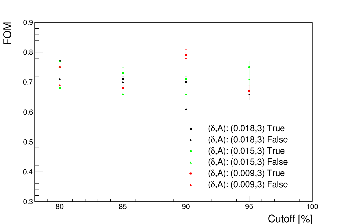
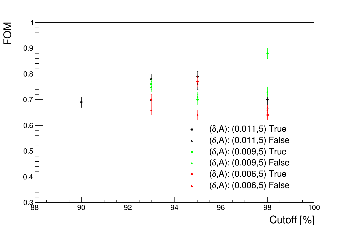
Figure 6: Evolution of the FOM as a function of the cutoff $C$ and for variable-fixing set to true (full circle) and false (full triangle). The QAML-Z algorithm uses the variable set A of Table 2. The left plot presents results for an augmentation scheme of ($\delta$,$A$)=(0.018,3) in black, (0.015,3) in green and (0.009,3) in red. The right plot shows results for ($\delta$,$A$)=(0.011,5) in black, (0.009,5) in green and (0.006,5) in red.

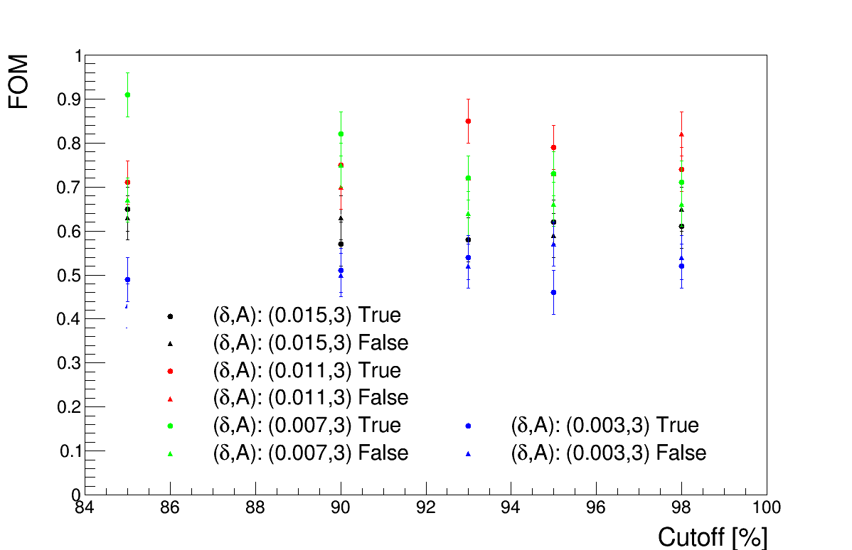
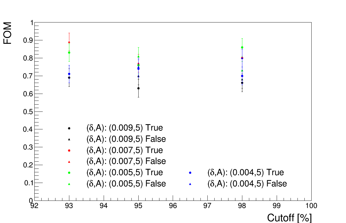
Figure 7: Evolution of the FOM as a function of the cutoff $C$ and for variable-fixing set to true (full circle) and false (full triangle). The QAML-Z algorithm uses the variable set B of Table 2. The left plot presents results for an augmentation scheme of ($\delta$,$A$)=(0.015,3) in black, (0.011,3) in red, (0.007,3) in green, and (0.003,3) in blue. The right plot shows results for ($\delta$,$A$)=(0.009,5) in black, (0.007,5) in red, (0.005,5) in green, and (0.004,5) in blue.

Appendix D Advanced variables

We construct new variables by performing operations between the discriminating variables of Table 1, where each new variable is built from two variables of this list. A two-dimensional distribution for each pair of initial variables allows to gauge the separation between signal and various background processes. Several analytic functions of the two variables are considered, and the one allowing to reach the highest FOM is retained per pair of variables. Seventeen new variables are constructed with this method, out of which nine are considered, see Table 4. Based on the discriminating power of each new variable, we consider two groups of variables, one made of the five new variables with the highest FOMs, and a second with the four subsequent ones.

Variables	FOM
$p_{\mathrm{T}}(l)$/$E_{\mathrm{T}}^{\mathrm{miss}}$	0.35
$p_{\mathrm{T}}(l)$/$p_{\mathrm{T}}(j_{1})$	0.22
($\mathrm{Disc(b)}$ $-$1)$p_{\mathrm{T}}(b)$	0.20
$|$($E_{\mathrm{T}}^{\mathrm{miss}}$$-$280)($M_{\mathrm{T}}$$-$80)$|$	0.20
$|$($E_{\mathrm{T}}^{\mathrm{miss}}$$-$280)($H_{\mathrm{T}}$$-$400)$|$	0.18
$\Delta R(l,b)$ $-$ ($M_{\mathrm{T}}$/40)	0.12
$H_{\mathrm{T}}$2/$N(\mathrm{jets})$	0.09
$p_{\mathrm{T}}$  $+$ 3.5$\eta(l)^{2}$	0.08
$p_{\mathrm{T}}$ /$H_{\mathrm{T}}$	0.03

Table 4: New discriminating variables constructed via operations on the ones of Table 1. For each new variable, the maximal value of the FOM is reported, where the corresponding uncertainty is negligible. Variables of Table 1 and those with higher FOMs (upper part) form the set A, while variables of the set A and those with lower FOMs (lower part) form the set B.

References

- [1] S. Chatrchyan, Phys. Lett. B 716, 30 (2012).
- [2] G. Aad, Phys. Lett. B 716, 1 (2012).
- [3] A. Mott, Nature 550, 375 (2017).
- [4] A. Zlokapa, Phys. Rev. A 102, 062405 (2020).
- [5] S. Chatrchyan, J. High Energy Phys. 09 065 (2018).
- [6] J. Shlens, arXiv:1404.1100.
- [7] J. Wess, Nuclear Phys. B70, 39 (1974).
- [8] R. Barbieri, Phys. Lett. B119, 343 (1982) 343.
- [9] H. O. Nilles, Phys. Rep. 110, 1 (1984).
- [10] H.E. Haber, Phys. Rep. 117, 75 (1985).
- [11] S. Dawson, Phys. Rev. D 31, 1581 (1985).
- [12] J.P. Martin, arXiv:9709356.
- [13] L. Rokach and O. Malmon, (World Scientific, Singapore, 2008), ISBN: 978-981-277-171-1.
- [14] H. Voss, Proc. Sci. ACAT2007 (2007) 040.
- [15] G. Cowan, K. Cranmer, E. Gross, and O. Vitells, Eur. Phys. J. C 71, 1554 (2011).
- [16] S. Chatrchyan, J. High Energy Phys. 07, 027 (2016).
- [17] P. I. Bunyk, IEEE Trans. Appl. Supercond. 24.4, 1 (2014).
- [18] J. Alwall, J. High Energy Phys. 07 (2014) 079.
- [19] T. Sjöstrand, J. High Energy Phys. 05 (2006) 026.
- [20] T. Sjöstrand, Comput. Phys. Commun. 178, 852 (2008).
- [21] J. de Favereau, J. High Energy Phys. 02 (2014) 57.
- [22] Joshua Job and Daniel Lidar, Sci. Technol. 3.3, 030501 (2018).
- [23] Davide Venturelli, Phys. Rev. X 5 031040 (2015).