Dynamic polarization of electron spins in indirect band gap (In,Al)As/AlAs quantum dots in weak magnetic field: experiment and theory

Abstract

A novel spin orientation mechanism — dynamic electron spin polarization has been recently suggested in Phys. Rev. Lett. 125, 156801 (2020). It takes place for unpolarized optical excitation in weak magnetic fields of the order of a few millitesla. In this paper we demonstrate experimentally and theoretically that the dynamic electron spin polarization degree changes sign as a function of time, strength of the applied magnetic field and its direction. The studies are performed on indirect band-gap (In,Al)As/AlAs quantum dots and their results are explained in the framework of a theoretical model developed for our experimental setting.

I Introduction

The manipulation of the spin degree of freedom in semiconductor nanostructures is interesting from the viewpoints of both basic physics Dyakonov ; Glazov and potential applications Dyakonov1 ; Fert . Generation of electron and hole spin polarization can be achieved in several ways. The main approaches to spin orientation are: optical spin orientation OO_book and thermal spin polarization in a magnetic field zeeman1897effect ; Shamirzaev60 ; Shamirzaev96 ; Shamirzaev94 . The first one is based on the transfer of the angular momentum from circularly polarized photons to electrons through the spin-orbit interaction. The second approach requires a lowering of the lattice temperature, so that the thermal energy becomes smaller than the electron Zeeman splitting. It can be enhanced in nonequilibrium conditions Ivchenko60 .

Recently we have suggested another approach to spin polarization: the dynamic electron spin polarization Smirnov125 . In contrast to the optical spin orientation, the proposed mechanism does not require circular polarization of the optical excitation. In contrast to the thermal spin polarization, we consider weak magnetic fields, for which the electron Zeeman splitting is much smaller than the thermal energy. This mechanism was approved experimentally for (In,Al)As/AlAs quantum dots (QDs) Smirnov125 .

In this paper, we extend these studies and present a deeper experimental and theoretical investigation of the dynamic electron spin polarization in indirect band gap (In,Al)As/AlAs QDs with type I band alignment. Namely, the dynamics of spin polarization in magnetic fields with different strength and orientation are studied. We find experimentally that the electron spin polarization degree changes sign with increasing delay time after pulsed excitation with unpolarized light or with the strength and orientation of the weak magnetic field. These experimental results agree with the developed microscopic theory based on the hyperfine interaction with nuclear spin fluctuations and the exchange interaction between electron and hole in an exciton confined in a QD.

The paper is organized as follows. In Sec. II the studied sample and the applied experimental techniques are described. In Sec. III we present the experimental results, before in Sec. IV we develop a theoretical model and describe general results obtained with the model. In Sec. V we compare the experiment and theory.

II Sample and experimental setup

The studied self-assembled (In,Al)As QDs embedded in an AlAs matrix were grown by molecular-beam epitaxy on a semi-insulating $(001)$-oriented GaAs substrate with a 400-nm-thick GaAs buffer layer Shamirzaev78 . The structure contains one QD layer sandwiched between two 70-nm-thick AlAs layers. The nominal amount of deposited InAs is about $2.5$ monolayers. The QDs were formed at the temperature 520^∘C with a growth interruption time of 20 s. The top AlAs barrier is protected from oxidation by a $20$-nm-thick GaAs cap layer. From the growth conditions and model calculations, we conclude that the average QD composition is In_0.75Al_0.25As Shamirzaev78 . The size and density of the lens-shaped QDs were measured by transmission electron microscopy, yielding an average diameter of 12 nm and a density of about 2$\times$10¹⁰ dots per cm². The relatively low QD density prevents carrier redistribution between the QDs ShamirzaevAPL97 ; ShamirzaevSST .

The sample was placed in a liquid helium bath cryostat. The temperature for all experiments was fixed at $T=1.8$ K. Low magnetic fields in the millitesla range were generated by an electromagnet. The angle $\theta$ between the magnetic field direction and the QD growth axis (z axis) was varied between 0^∘ (Faraday geometry) and 90^∘ (Voigt geometry). For measurement of angular dependencies we fixed the magnetic field direction and rotated the sample. The emission was collected either in the direction along the field axis in Faraday geometry for $0^{\circ}\leq\theta\leq 45^{\circ}$ or perpendicular to the field axis in Voigt geometry for $45^{\circ}\leq\theta\leq 90^{\circ}$.

The photoluminescence (PL) was excited nonresonantly with the laser photon energy exceeding the direct band gap of the AlAs matrix, which is equal to 3.099 eV Vurgaftman . We used the third harmonic of a Q-switched Nd:YVO₄ pulsed laser with a photon energy of $3.49$ eV, a pulse duration of $5$ ns and a repetition rate of 1 kHz Shamirzaev84 . The exciting light was linearly polarized, and we checked that the direction of the polarization does not affect the presented results, as expected for strongly nonresonant excitation. The PL was dispersed by a $0.5$-m monochromator. For the time-resolved and time-integrated PL measurements we used a gated charge-coupled-device (CCD) camera, synchronized with the laser via an external trigger signal. The time delay between the pump pulse and the start of PL recording, $t_{\text{d}}$, was varied from zero up to $1$ ms. The duration of PL recording, i.e., the gate window $t_{\text{g}}$ was varied from $1$ ns to $1$ ms. The signal intensity and the time resolution of the setup depend on $t_{\text{d}}$ and $t_{\text{g}}$. The highest time resolution of the detection system is $1$ ns.

The circularly polarized components of the emission were selected by combining Glan-Thompson prisms and quarter-wave plates. The circular polarization degree of the PL is given by $P_{c}=(I_{+}-I_{-})/(I_{+}+I_{-})$, where $I_{+}$ and $I_{-}$ are the intensities of the $\sigma^{+}$ and $\sigma^{-}$ polarized PL components, respectively. To determine the sign of $P_{c}$, we performed a control measurement on a diluted magnetic semiconductor structure with (Zn,Mn)Se/(Zn,Be)Se quantum wells. For this structure, it is known that $P_{c}>0$ for $B_{z}>0$ in Faraday geometry Keller .

III Experimental results

The dispersion in QD size, shape, and composition within the ensemble leads to the formation of (In,Al)As/AlAs QDs with different band structure, as shown in Fig. 1(a). The electron ground state changes from the $\Gamma$ to the X valley with decrease of the dot size, while the heavy-hole (hh) ground state remains at the $\Gamma$ point. This corresponds to a change from a direct to an indirect band gap. On the other hand, the type-I band alignment is preserved, that is, in both cases, electron and hole are spatially confined within the (In,Al)As QDs Shamirzaev78 ; Shamirzaev84 ; ShamirzaevAPL92 . Note that the change of electron ground state from a direct to an indirect band with decreasing QDs size is not unique for (In,Al)As/AlAs QDs, it was demonstrated for various semiconductor heterostructures Cedric1 ; Cedric2 ; Apex ; Shamirzaev45 ; Abramkin53 ; Pistol ; Shamirzaev97 .

Recently, we demonstrated that the coexistence of (In,Al)As/AlAs QDs with direct and indirect band gaps in the ensemble is evidenced by the spectral dependence of the exciton recombination time Shamirzaev78 ; Shamirzaev84 ; ShamirzaevAPL92 . In direct QDs, the excitons recombine within a few nanoseconds Rautert100 . On the contrary, the indirect QDs are characterized by long decay times due to their small exciton oscillator strength. Here, we use accordingly time-resolved photoluminescence to identify indirect band-gap QDs.

III.1 Time-resolved photoluminescence

Photoluminescence spectra of an (In,Al)As/AlAs QD ensemble measured for nonresonant excitation are shown in Fig. 1(b). The time-integrated spectrum (black line) has a maximum at 1.67 eV and extends from 1.50 eV (at lower energies the PL is related to the GaAs substrate) to 1.90 eV, with a full width at half maximum (FWHM) of about 190 meV. The large width of the emission band is due to the dispersion of the QD parameters, since the exciton energy depends on QD size, shape and composition Shamirzaev78 . The PL band is contributed by the emission of direct and indirect QDs, as becomes evident from the time-resolved PL spectra. For the spectrum measured immediately after the laser pulse ($t_{\text{d}}=1$ ns and $t_{\text{g}}=4$ ns), the PL band (red line) has its maximum at 1.59 eV and a FWHM of 100 meV. For longer delays ($t_{\text{d}}=1~{}\mu$s and $t_{\text{g}}=5~{}\mu$s), the emission maximum shifts to 1.68 eV and the band broadens to 180 meV (blue line), rather similar to the time-integrated PL spectrum. We recently demonstrated that after photoexcitation in the AlAs barriers electrons and holes are captured in QDs within several picoseconds, and the capture probability does not depend on the QD size and composition ShamirzaevNT . Therefore, all QDs in the ensemble (direct and indirect) become equally populated shortly after the excitation pulse.

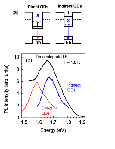
Figure 1: (a) Band diagrams of (In,Al)As/AlAs QDs with direct and indirect band structure. (b) Photoluminescence spectra of (In,Al)As/AlAs QDs measured for non-resonant excitation: time-integrated (black line), time-resolved for $t_{\text{d}}=1$ ns and $t_{\text{g}}=4$ ns (red), as well as for $t_{\text{d}}=1~{}\mu$s and $t_{\text{g}}=5~{}\mu$s (blue).

Thus, the exciton recombination dynamics is fast for direct QDs emitting mainly in the spectral range of $1.50-1.70$ eV and slow for the indirect QDs emitting in the range of $1.60-1.90$ eV. The emission of the direct and indirect QDs overlaps in the range of $1.60-1.70$ eV.

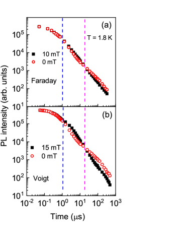
Figure 2: Dynamics of unpolarized PL for indirect excitons at the energy of $1.67$ eV in zero (open red circles) and weak magnetic fields (filled black squares) for (a) Faraday and (b) Voigt geometry. Dashed vertical lines show delay times after excitation pulse $t_{\text{d1}}$ (blue) and $t_{\text{d2}}$ (magenta). Note the bilogarithmic scale.

The dynamics of the unpolarized PL (sum of the $\sigma^{+}$ and $\sigma^{-}$ polarized PL components) measured for indirect QDs at 1.67 eV in zero and in weak longitudinal and transverse magnetic fields are shown in Figs. 2(a) and 2(b), respectively. The data are plotted in bilogarithmic scale, which is convenient for presenting the dynamics across a wide range of decay times and PL intensities. The decay curves are non-exponential. Such a dynamics results from superposition of multiple monoexponential decays of single QDs Rautert100 with different decay times varying with size, shape, and composition of the QDs Shamirzaev84 .

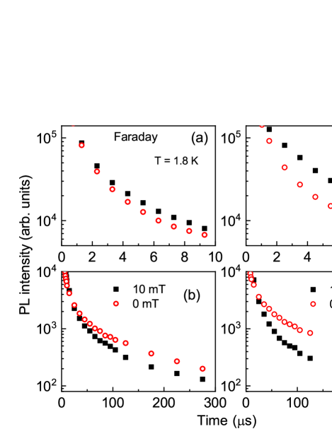
Figure 3: Dynamics of unpolarized PL for indirect excitons at the energy of $1.67$ eV in zero (open red circles) and weak magnetic fields (filled black squares) selected for different ranges of delay times after the excitation pulse: (a) $0-t_{\text{d2}}$, (b) $t_{\text{d2}}-t_{\text{dmax}}$ for Faraday geometry, and (c) $0-t_{\text{d2}}$, (d) $t_{\text{d2}}-t_{\text{dmax}}$ for Voigt geometry.

One can see that even a very weak magnetic field of 10 mT influences the exciton recombination dynamics in both field orientations. The three specific stages are separated in Fig. 2 by vertical dashed lines for both Faraday and Voigt geometries. At the first stage before $t_{\text{d}1}=1~{}\mu$s, the PL does not depend on magnetic field. In order to have a closer look at the following dynamic stages we present them separately in Fig. 3. In both cases of Faraday and Voigt geometries, at the second stage for $t_{\text{d}}$ between $t_{\text{d1}}$ and $t_{\text{d2}}=20~{}\mu$s the magnetic field boosts the PL [Figs. 3(a) and 3(c)], while at the third stage, $t_{\text{d}}>t_{\text{d2}}$, the PL intensity decreases with field application [Figs. 3(b) and 3(d)].

The effect of the magnetic field on the PL decay can be estimated quantitatively, because it is characterized by the difference of PL intensities, $I_{PL}$, integrated between $t_{\text{d1}}$ and $t_{\text{d2}}$ for the second stage and between $t_{\text{d2}}$ and the maximum delay $t_{\text{dmax}}$ for the third stage, with applied field and without the field. To compare the cases of longitudinal and transverse magnetic field, these differences have to be normalized by the integrated intensity of the PL without field as follows:

$$S2=\frac{\int_{t_{\text{d1}}}^{t_{\text{d2}}}I_{PL}(t,B)dt-\int_{t_{\text{d1}}}^{t_{\text{d2}}}I_{PL}(t,B=0)dt}{\int_{t_{\text{d1}}}^{t_{\text{d2}}}I_{PL}(t,B=0)dt},$$ (1)

$$S3=\frac{\int_{t_{\text{d2}}}^{t_{\text{dmax}}}I_{PL}(t,B)dt-\int_{t_{\text{d2}}}^{t_{\text{dmax}}}I_{PL}(t,B=0)dt}{\int_{t_{\text{d2}}}^{t_{\text{dmax}}}I_{PL}(t,B=0)dt}.$$

The calculations show that S2 equals $85$ and $325$, and S3 equals $-77$ and $-170$ for Faraday and Voigt geometry, respectively. Note that the magnetic field induces mostly a change in dymanics, while the decrease of the total PL intensity integrated from $t=0$ to $t_{\text{dmax}}$ in magnetic field is small, amounting to 1.8$\%$ in Faraday and 5.0$\%$ in Voigt geometries.

III.2 Magnetic-field-induced circular polarization of photoluminescence

A very weak (in the few millitesla range) longitudinal magnetic field leads to the appearance of dynamic electron spin polarization Smirnov125 , which can be evidenced in the circular polarization of the photoluminescence. At fixed magnetic field, the sign of the polarization and the polarization degree depend on the delay after the excitation pulse. This is shown in Fig. 4, which demonstrates PL spectra measured at $B_{z}=10$ mT in $\sigma^{+}$ and $\sigma^{-}$ polarization for different sets of $t_{\text{d}}$ and $t_{\text{g}}$. One can see that the PL is unpolarized at $t_{\text{d}}=$ 0.7 $\mu$s, gets negatively polarized at $t_{\text{d}}=7~{}\mu$s, again loses polarization at $t_{\text{d}}=50~{}\mu$s, but becomes positively polarized at $t_{\text{d}}=250~{}\mu$s.

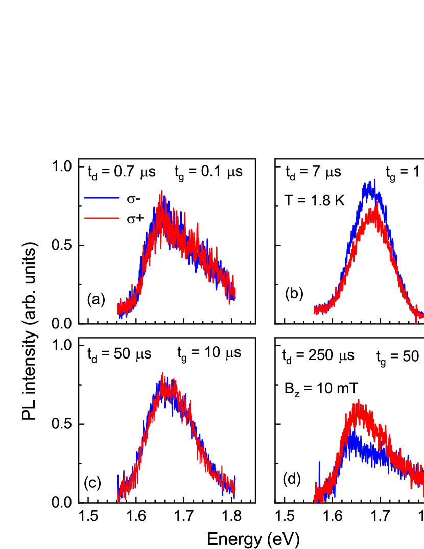
Figure 4: PL spectra measured for opposite circular polarizations in longitudinal magnetic field $B_{z}=10$ mT, for the experimental settings: (a) $t_{\rm d}=0.7$ $\mu$s and $t_{\rm g}=0.1$ $\mu$s; (b) $t_{\rm d}=7$ $\mu$s and $t_{\rm g}=1$ $\mu$s; (c) $t_{\rm d}=50$ $\mu$s and $t_{\rm g}=10$ $\mu$s; and (d) $t_{\rm d}=250$ $\mu$s and $t_{\rm g}=50$ $\mu$s.

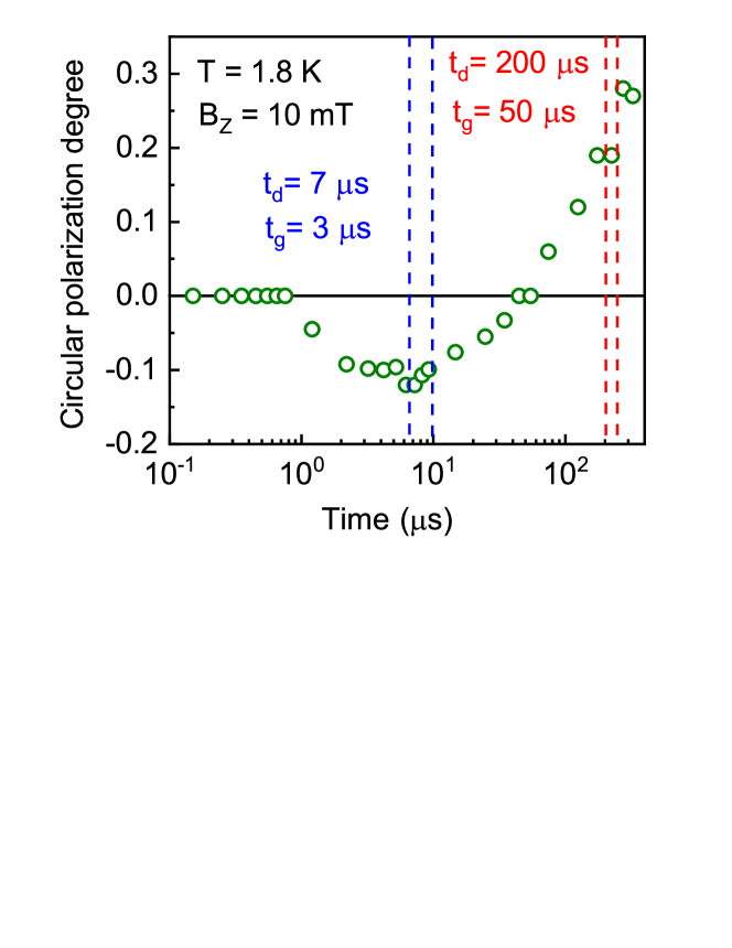
Figure 5: Dynamics of PL circular polarization degree measured at the energy of $1.67$ eV for the magnetic field $B_{z}=10$ mT in Faraday geometry. Vertical lines show the time-integration windows for Fig. 6.

The dynamics of the PL circular polarization degree detected at the energy of $1.67$ eV for $B_{z}=10$ mT is shown in Fig. 5. The negative polarization appears at a delay of about 1 $\mu$s after the pump pulse, the polarization degree decreases and reaches $-0.12$ at the delay of 8 $\mu$s, then increases to zero for a delay of 50 $\mu$s. At large delays, the polarization changes sign (becomes positive), the polarization degree increases monotonically and finally reaches 0.28 at the delay of 300 $\mu$s.

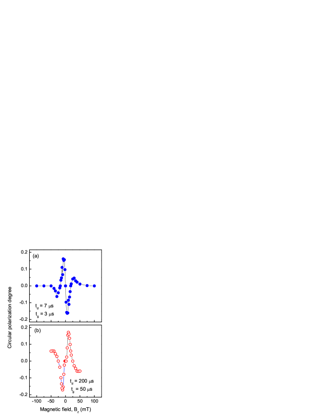
Figure 6: Circular polarization degree of the PL at the energy of $1.66$ eV integrated in the time windows shown in Fig. 5 in Faraday geometry as a function of magnetic field: (a) $t_{\rm d}=7$ $\mu$s and $t_{\rm g}=3$ $\mu$s, (b) $t_{\rm d}=200$ $\mu$s and $t_{\rm g}=50$ $\mu$s.

The magnetic field dependencies of the polarization degree of the PL integrated for the two time windows shown by the vertical dashed lines in Fig. 5, which correspond to negative and positive PL polarizations are shown in Figs. 6(a) and 6(b), respectively. First of all, it should be noted that both dependencies are: (i) odd as function of the magnetic field and (ii) strongly non-monotonic, almost quasi-oscillatory.

For the parameters $t_{\rm d}=7$ $\mu$s and $t_{\rm g}=3$ $\mu$s corresponding to the negative circular polarization range of the PL [Fig. 6(a)] the polarization degree decreases to $-0.16$ in $B_{z}=6$ mT, and then increases to zero, changes sign, reaches 0.06 at 30 mT field, and then drops to zero at fields larger than 50 mT. For the delay range corresponding to the positive circular polarization of PL at $10$ mT ($t_{\rm d}=200$ $\mu$s and $t_{\rm g}=50$ $\mu$s) [Fig. 6(b)], the $P_{c}(B)$ shows a qualitatively similar behavior.

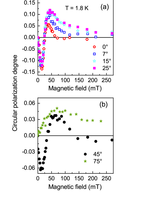
Figure 7: Circular polarization degree of PL at the energy of $1.70$ eV integrated in the time window with $t_{\rm d}=5$ $\mu$s and $t_{\rm g}=5$ $\mu$s as function of magnetic field for different angles between the magnetic field direction and the QD growth axis, $\theta$: (a) 0^∘ - Faraday geometry (open red circles), 7^∘ (open blue squares), 15^∘ (open cyan stars) and 25^∘ (filled magenta squares); (b) 45^∘ (black circles), and 75^∘ (green stars).

A change in the angle $\theta$ between the magnetic field direction and the QD growth axis modifies the dependence of the PL circular polarization degree on the magnetic field strength. The $P_{c}(B)$ measured for the settings $t_{\rm d}=5$ $\mu$s and $t_{\rm g}=5$ $\mu$s, corresponding to the negative circular polarization range of the PL, are shown in Figs. 7(a) and 7(b) for different angles $\theta$ in the range $0^{\circ}\leq\theta\leq 75^{\circ}$. One can see that in the angle range $0^{\circ}\leq\theta\leq 25^{\circ}$ the negatively polarized part of the $P_{c}(B)$ curve practically does not change, while for the positively polarized PL the polarization degree increases and the maximum of $P_{c}(B)$ shifts towards stronger magnetic fields. A further increase of the $\theta$ angle leads to a decrease of the polarization degree of both the negatively and positively polarized PL. However, the decrease of the polarization degree of the negatively polarized PL is faster than that of the positively polarized one. In fact, the negatively polarized part of $P_{c}(B)$ completely disappears for $\theta$ above $60^{\circ}$, while we observe positively polarized PL up to angles of $75^{\circ}$.

Let us summarize the most important experimental findings:

(i) The application of a weak magnetic field (in both Faraday and Voigt geometry), modifies the dynamics of the unpolarized PL resulting in accelerated or decelerated decay in different time ranges, but does not change the integral of the PL intensity. The effect is similar for both field orientations, but more pronounced in the Voigt geometry.

(ii) A weak longitudinal magnetic field (Faraday geometry) induces a circular polarization of the photoluminescence.

(iii) The dynamics of this polarization degree is strongly non-monotonic in time. After the excitation pulse it first equals to zero, then the polarization degree becomes negative, drops subsequently again to zero, changes it sign (from negative to positive) and finally strongly increases.

(iv) For any delay time after the excitation pulse, either with positive or negative PL polarization, the polarization degree is an odd function of the magnetic field and varies strongly non-monotonic with magnetic field strength. The polarization degree increases in very small fields up to a maximum value, then with rising field decreases to zero, changes its sign and increases again. A further increase in field strength again leads to a drop of the polarization degree down to zero.

(v) A change of the angle $\theta$ between the magnetic field direction and the QD growth axis modifies the dependence of the PL circular polarization degree on the magnetic field strength. The positively polarized PL is maintained up to large angles $\theta$, while the negatively polarized PL observed for $\theta=0^{\circ}$ disappears in weak magnetic fields.

IV Theory

In this section we develop a microscopic theory of the dynamic electron spin polarization in quantum dots and its detection through polarization resolved exciton photoluminescence. We present an extension of our model from Ref. Smirnov125, , considering first a set of identical QDs. The luminescence of different QDs is considered to be independent. In the next Sec. V a set of different QDs will be considered to describe the experimental results.

IV.1 Model

An exciton consists of a heavy hole with the spin projections $J_{z}=\pm 3/2$ along the structure growth axis $z$ and an electron with the spin projections $S_{z}=\pm 1/2$. We account for the external magnetic field, the hyperfine interaction between the electron spin and the unpolarized spins of the nuclei in the QD, and the short range exchange interaction between the electron and hole spins.

The system Hamiltonian can be written as

$$\mathcal{H}=\hbar\bm{\Omega}_{\rm tot}\bm{S},$$ (2)

where

$$\bm{\Omega}_{\rm tot}=\bm{\Omega}_{L}+\bm{\Omega}_{\rm Nf}+\bm{\Omega}_{\rm ex}$$ (3)

is the total electron spin precession frequency. Here, $\bm{\Omega}_{L}$ is the electron Larmor spin precession frequency in the external magnetic field $\bm{B}=\hbar\bm{\Omega}_{L}/(g_{e}\mu_{B})$ with $g_{e}$ being the electron $g$ factor and $\mu_{B}$ being the Bohr magneton, $\bm{\Omega}_{\rm Nf}$ is the precession frequency in the Overhauser field of the randomly oriented nuclear spins in the QD, $\bm{\Omega}_{\rm ex}=-\frac{2}{3}\delta_{0}J_{z}\bm{e}_{z}/\hbar$ is the precession frequency in the exchange field of the heavy hole, with $\delta_{0}$ being the short range exchange interaction constant Ivch_book ; Astakhov and $\bm{e}_{z}$ being the unit vector along the $z$ axis. Noteworthy, due to this term the total electron spin precession frequency depends on the hole spin $J_{z}$, as it is shown in Fig. 8.

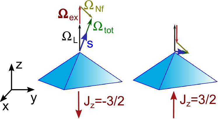
Figure 8: Electron spin precession frequency $\bm{\Omega}_{\rm tot}$ [Eq. (3)] and the contributions to it for the two heavy hole spin orientations. The average electron spin $\bm{S}$ is parallel to $\bm{\Omega}_{\rm tot}$ due to fast precession.

For simplicity we neglect a number of contributions in the Hamiltonian. First, we neglect the long range electron hole exchange interaction, which is suppressed for the indirect excitons Bir ; Goupalov ; Kuznetsova as well as possible noncollinear terms in the short range exchange interaction for electrons in the $X$ valley. We also neglect the hole Zeeman splitting, because the transverse components of the tensor of the heavy hole $g$ factors are very small Debus ; Golub , while the longitudinal component does not play a role in the phenomena addressed here Smirnov125 . For the same reasons we neglect the hyperfine interaction for the hole, which is additionally suppressed by the p-type orbitals of the Bloch wave functions Glazov ; Chekhovich . For the electrons we neglect the possible valley degeneracy and assume that the electron spin dynamics take place only within one of the valleys, while in general the hyperfine interaction can scatter electrons between the valleys Avdeev , which can lead to spin relaxation. For simplicity we neglect the nuclear spin polarization OO_book ; Korenev and nuclear spin dynamics, which in principle can take place at submillisecond time scale Petrov ; Inertia ; CSM . Further, we neglect the anisotropy of the hyperfine interaction Shchepetilnikov ; Kuznetsova , and assume that the distribution function of the Overhauser field has the form Merkulov ; PRC_general :

$$\mathcal{F}({\bm{B}}_{\rm Nf})=\frac{1}{(\sqrt{\pi}\Delta_{B})^{3}}\exp\left(-\frac{{B}_{\rm Nf}^{2}}{\Delta_{B}^{2}}\right),$$ (4)

where the parameter $\Delta_{B}$ characterizes the dispersion of the Overhauser field. Thus, the exciton spin dynamics due to the hyperfine interaction is reduced to precession with a static frequency $\bm{\Omega}_{\rm Nf}=\mu_{B}g_{e}{\bm{B}}_{\rm Nf}/\hbar$, and the spin dynamics should be averaged over the distribution $\mathcal{F}({\bm{B}}_{\rm Nf})$.

Since $J_{z}$ is a good quantum number, it is useful to introduce $N^{(+)}$ and $N^{(-)}$ as the numbers of excitons with hole spin projections $+3/2$ and $-3/2$, respectively relations . We also introduce the averaged spin polarizations ${\bm{S}}^{(\pm)}$ of the electrons in the excitons with $J_{z}=\pm 3/2$. Then the exciton dynamics including incoherent processes is described by the following equations:

$$\frac{dN^{(\pm)}}{dt}=-\frac{1}{\tau_{R}}\left(\frac{N^{(\pm)}}{2}\mp S_{z}^{(\pm)}\right)-\frac{1}{\tau_{NR}}\left(\frac{N^{(\pm)}}{2}\pm S_{z}^{(\pm)}\right)+\frac{N^{(\mp)}-N^{(\pm)}}{2\tau_{s}^{h}}+\left(\frac{1}{\tau_{1}}+\frac{1}{\tau_{2}}\right)\frac{N^{(\mp)}-N^{(\pm)}}{4}\\ \pm\left(\frac{1}{\tau_{1}}-\frac{1}{\tau_{2}}\right)\frac{S_{z}^{(+)}+S_{z}^{(-)}}{2},$$ (5a)

$$\frac{dS_{z}^{(\pm)}}{dt}=\pm\left(\frac{1}{\tau_{R}}-\frac{1}{\tau_{NR}}\right)\frac{N^{(\pm)}}{4}-\left(\frac{1}{\tau_{s}^{e}}+\frac{1}{2\tau_{R}}+\frac{1}{2\tau_{NR}}\right)S_{z}^{(\pm)}+\frac{S_{z}^{(\mp)}-S_{z}^{(\pm)}}{2\tau_{s}^{h}}+[\bm{\Omega}_{\rm tot}^{(\pm)}\times{\bm{S}}^{(\pm)}]_{z}\\ -\left(\frac{1}{\tau_{1}}+\frac{1}{\tau_{2}}\right)\frac{S_{z}^{(+)}+S_{z}^{(-)}}{4}+\left(\frac{1}{\tau_{1}}-\frac{1}{\tau_{2}}\right)\frac{N^{(+)}-N^{(-)}}{8},$$ (5b)

$$\frac{dS_{x,y}^{(\pm)}}{dt}=-\left(\frac{1}{\tau_{s}^{e}}+\frac{1}{2\tau_{R}}+\frac{1}{2\tau_{NR}}+\frac{1}{2\tau_{1}}+\frac{1}{2\tau_{2}}\right)S_{x,y}^{(\pm)}+\frac{S_{x,y}^{(\mp)}-S_{x,y}^{(\pm)}}{2\tau_{s}^{h}}+[\bm{\Omega}_{\rm tot}^{(\pm)}\times{\bm{S}}^{(\pm)}]_{x,y}.$$ (5c)

Here ${\bm{\Omega}}_{\rm tot}^{(\pm)}=\bm{\Omega}_{L}+\bm{\Omega}_{\rm Nf}\mp\delta_{0}\bm{e}_{z}/\hbar$ is the vector frequency of the electron spin precession corresponding to the hole spin projections $J_{z}=\pm 3/2$, $\tau_{s}^{e}$ and $\tau_{s}^{h}$ are the electron and hole spin relaxation times, respectively, $\tau_{1}$ and $\tau_{2}$ are the bright and dark excitons spin flip times, and $\tau_{R}$ and $\tau_{NR}$ are the lifetimes of the bright and dark excitons related to radiative and nonratiative recombination. The action of the spin relaxation terms is illustrated in Fig. 9.

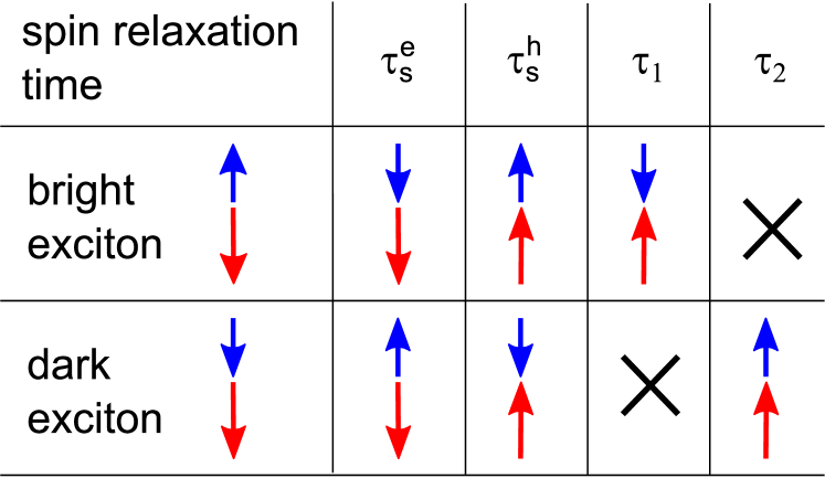
Figure 9: The action of the different spin relaxation mechanisms described by the times $\tau_{s}^{e}$, $\tau_{s}^{h}$, $\tau_{1}$, and $\tau_{2}$ on the electron (blue arrow) and hole (red arrow) spin projections onto the $z$ axis inside the bright and dark excitons. The initial states and the results of the action are shown in the first and the corresponding columns, respectively. The spin relaxations described by the times $\tau_{1}$ and $\tau_{2}$ do not affect the dark and bright states, respectively.

Pulsed unpolarized optical excitation is described by the initial conditions $N^{(\pm)}=N_{0}/2$ with $N_{0}$ being the number of generated excitons and $\bm{S}^{(\pm)}=0$. The PL intensities in $\sigma^{\pm}$ polarization are proportional to

$$R_{\pm}=\frac{N^{(\pm)}/2\mp S_{z}^{(\pm)}}{\tau_{R}},$$ (6)

respectively. The degree of the circular polarization is given by

$$P=\frac{\braket{R_{+}-R_{-}}}{\braket{R_{+}+R_{-}}},$$ (7)

where the angular brackets denote the averaging at the given time over the random nuclear fields.

The electron spin precession is typically much faster than all the the incoherent processes. So we use the adiabatic approximation and replace the electron spins $\bm{S}^{(\pm)}$ with their values averaged over the precession period, which are parallel to $\bm{\Omega}_{\rm tot}^{(\pm)}$. Then, it is useful to introduce

$${\cal B}^{(\pm)}=\frac{1}{2}N^{(\pm)}\mp{\bm{S}}^{(\pm)}{\bm{e}}_{\Omega}^{(\pm)},$$ (8)

$${\cal D}^{(\pm)}=\frac{1}{2}N^{(\pm)}\pm{\bm{S}}^{(\pm)}{\bm{e}}_{\Omega}^{(\pm)},$$ (9)

with ${\bm{e}}_{\Omega}^{(\pm)}={\rm sign}\left[(\Omega_{\rm tot}^{(\pm)})_{z}\right]\cdot{\bm{\Omega}}_{\rm tot}^{(\pm)}/|{\bm{\Omega}}_{\rm tot}^{(\pm)}|$ being the unit vector along $\bm{\Omega}_{\rm tot}^{(\pm)}$ with positive $z$ component. So ${\cal B}^{(\pm)}$ and ${\cal D}^{(\pm)}$ have the meaning of the numbers of mainly bright and mainly dark excitons with the electron spin being parallel to its precession frequency. If ${\bm{\Omega}}_{\rm tot}$ is parallel to the $z$ axis, they are equal to the number of the corresponding bright and dark excitons. These excitons are called quasi bright and quasi dark, respectively, in the following.

For infinite $\tau_{1}$ and $\tau_{2}$, we obtain the following kinetic equations for the numbers of quasi bright and quasi dark excitons:

$$\frac{d{\cal B}^{(\pm)}}{dt}=-\left(\frac{1+\cos\alpha_{\pm}}{\tau_{R}}+\frac{1-\cos\alpha_{\pm}}{\tau_{NR}}+\frac{1}{\tau_{s}^{e}}+\frac{1}{\tau_{s}^{h}}\right)\frac{{\cal B}^{(\pm)}}{2}+\frac{{\cal D}^{(\pm)}}{2\tau_{s}^{e}}+\frac{1-\cos\beta}{4\tau_{s}^{h}}{\cal B}^{(\mp)}+\frac{1+\cos\beta}{4\tau_{s}^{h}}{\cal D}^{(\mp)},$$ (10)

$$\frac{d{\cal D}^{(\pm)}}{dt}=-\left(\frac{1-\cos\alpha_{\pm}}{\tau_{R}}+\frac{1+\cos\alpha_{\pm}}{\tau_{NR}}+\frac{1}{\tau_{s}^{e}}+\frac{1}{\tau_{s}^{h}}\right)\frac{{\cal D}^{(\pm)}}{2}+\frac{{\cal B}^{(\pm)}}{2\tau_{s}^{e}}+\frac{1+\cos\beta}{4\tau_{s}^{h}}{\cal B}^{(\mp)}+\frac{1-\cos\beta}{4\tau_{s}^{h}}{\cal D}^{(\mp)}.$$ (11)

Here $\alpha_{\pm}$ is the angle between the axes of ${\bm{\Omega}}_{\rm tot}^{(\pm)}$ and the $z$ axis, and $\beta$ is the angle between the axes of ${\bm{\Omega}}_{\rm tot}^{(\pm)}$. Importantly, these are the angles between the axes and not between the directions, so $0\leq\alpha_{\pm}$ and $\beta\leq\pi/2$. We note that after a hole spin flip occuring on the typical time scale of $\tau_{s}^{h}$, the quasi bright exciton with $J_{z}=+3/2$ becomes an exciton with hole spin $-3/2$ and since the effective fields ${\bm{\Omega}}_{\rm tot}^{(\pm)}$ are different, the exciton remains quasi bright with the probability $(1-\cos\beta)/2$ and becomes quasi dark with the probability $(1+\cos\beta)/2$. The terms corresponding to the other processes can be described in the same way.

The terms related to $\tau_{1}$ and $\tau_{2}$ give the following contributions to ${d{\cal B}^{(\pm)}}/{dt}$ and ${d{\cal D}^{(\pm)}}/{dt}$, respectively:

$$\left(\frac{d{\cal B}^{(\pm)}}{dt}\right)^{\prime}=-\left(\frac{1}{\tau_{1}}-\frac{(1-\cos\alpha_{\pm})^{2}}{4\tau_{1}}+\frac{1}{\tau_{2}}-\frac{(1+\cos\alpha_{\pm})^{2}}{4\tau_{2}}\right)\frac{{\cal B}^{(\pm)}}{2}+\left(\frac{1}{\tau_{1}}+\frac{1}{\tau_{2}}\right)\frac{\sin^{2}\alpha_{\pm}}{8}{\cal D}^{(\pm)}\\ +\frac{(1+\cos\alpha_{\pm})(1+\cos\alpha_{\mp})}{8\tau_{1}}{\cal B}^{(\mp)}+\frac{(1-\cos\alpha_{\pm})(1-\cos\alpha_{\mp})}{8\tau_{2}}{\cal B}^{(\mp)}\\ +\frac{(1+\cos\alpha_{\pm})(1-\cos\alpha_{\mp})}{8\tau_{1}}{\cal D}^{(\mp)}+\frac{(1-\cos\alpha_{\pm})(1+\cos\alpha_{\mp})}{8\tau_{2}}{\cal D}^{(\mp)},$$ (12a)

$$\left(\frac{d{\cal D}^{(\pm)}}{dt}\right)^{\prime}=-\left(\frac{1}{\tau_{1}}-\frac{(1+\cos\alpha_{\pm})^{2}}{4\tau_{1}}+\frac{1}{\tau_{2}}-\frac{(1-\cos\alpha_{\pm})^{2}}{4\tau_{2}}\right)\frac{{\cal D}^{(\pm)}}{2}+\left(\frac{1}{\tau_{1}}+\frac{1}{\tau_{2}}\right)\frac{\sin^{2}\alpha_{\pm}}{8}{\cal B}^{(\pm)}\\ +\frac{(1-\cos\alpha_{\pm})(1+\cos\alpha_{\mp})}{8\tau_{1}}{\cal B}^{(\mp)}+\frac{(1+\cos\alpha_{\pm})(1-\cos\alpha_{\mp})}{8\tau_{2}}{\cal B}^{(\mp)}\\ +\frac{(1-\cos\alpha_{\pm})(1-\cos\alpha_{\mp})}{8\tau_{1}}{\cal D}^{(\mp)}+\frac{(1+\cos\alpha_{\pm})(1+\cos\alpha_{\mp})}{8\tau_{2}}{\cal D}^{(\mp)}.$$ (12b)

To interpret these contributions, let us consider, for example, the terms in Eqs. (12) that are related to the spin flip of the dark exciton with $J_{z}=+3/2$ described by the time $\tau_{2}$. One can say that with the rate $1/(2\tau_{2})$ it becomes either dark with the probability $(1+\cos\alpha_{+})/2$ or bright with the probability $(1-\cos\alpha_{+})/2$. If it became dark, it has changed the direction of both the electron and hole spins. Then due to the fast electron spin precession it contributes to ${\cal D}^{(-)}$ with the probability $(1+\cos\alpha_{-})/2$ or to ${\cal B}^{(-)}$ with the probability $(1-\cos\alpha_{-})/2$. At the same time, the bright exciton does not change its spin because $\tau_{2}$ is relevant for the dark excitons only, so it contributes to ${\cal D}^{(+)}$ with the probability $(1-\cos\alpha_{+})/2$ and to ${\cal B}^{(+)}$ with the probability $(1+\cos\alpha_{+})/2$. The rest of the terms can be interpreted in the same way.

The circularly polarized PL components in this limit are described by

$$R_{\pm}=\frac{1+\cos\alpha_{\pm}}{2\tau_{R}}{\cal B}^{(\pm)}+\frac{1-\cos\alpha_{\pm}}{2\tau_{R}}{\cal D}^{(\pm)}.$$ (13)

It is instructive to consider the absence of hole spin relaxation as well as bright and dark exciton spin flips. In this case, the hole spin is conserved, so Eqs. (11) and (10) are reduced to the two independent sets of equations:

$$\frac{d}{dt}\left(\begin{array}[]{c}{\cal D}^{(\pm)}\\ {\cal B}^{(\pm)}\end{array}\right)=\left(-\frac{1}{2\tau_{0}}-\frac{1}{2\tau_{s}^{e}}+M^{\pm 3/2}\right)\left(\begin{array}[]{c}{\cal D}^{(\pm)}\\ {\cal B}^{(\pm)}\end{array}\right),$$ (14)

with the matrices

$$M^{\pm 3/2}=\left(\begin{array}[]{cc}\frac{1}{2\tau_{\alpha}}\cos\alpha_{\pm}&\frac{1}{2\tau_{s}}\\ \frac{1}{2\tau_{s}}&-\frac{1}{2\tau_{\alpha}}\cos\alpha_{\pm}\end{array}\right).$$ (15)

Here $\tau_{0}=\tau_{R}\tau_{NR}/(\tau_{R}+\tau_{NR})$ and $\tau_{\alpha}=\tau_{R}\tau_{NR}/(\tau_{NR}-\tau_{R})$. These matrices have the eigenvalues $\gamma_{\pm}$ and $-\gamma_{\pm}$, respectively, where $\gamma_{\pm}=\sqrt{\tau_{s}^{2}\cos^{2}\alpha_{\pm}+\tau_{\alpha}^{2}}/2\tau_{s}\tau_{\alpha}$. Therefore, the PL dynamics is biexponential:

$$R_{\pm}(t)=\exp\left(-\frac{t}{2\tau_{s}}-\frac{t}{2\tau_{\alpha}}\right)\times\\ \left(R_{\pm}^{(1)}e^{-\gamma_{\pm}t}+R_{\pm}^{(2)}e^{\gamma_{\pm}t}\right),$$ (16)

where

$$R_{\pm}^{(1)}=\frac{1}{2\tau_{R}}\left[\frac{(\xi_{\pm}+\tau_{\alpha})^{2}}{\tau_{\alpha}^{2}+\xi_{\pm}^{2}}+\frac{\tau_{\alpha}^{2}-\xi_{\pm}^{2}}{\tau_{\alpha}^{2}+\xi_{\pm}^{2}}\cos\alpha_{\pm}\right],$$ (17)

$$R_{\pm}^{(2)}=\frac{1}{2\tau_{R}}\left[\frac{(\zeta_{\pm}+\tau_{\alpha})^{2}}{\tau_{\alpha}^{2}+\zeta_{\pm}^{2}}+\frac{\tau_{\alpha}^{2}-\zeta_{\pm}^{2}}{\tau_{\alpha}^{2}+\zeta_{\pm}^{2}}\cos\alpha_{\pm}\right]$$ (18)

with $\xi_{\pm}=\tau_{s}(\cos\alpha_{\pm}-2\tau_{\alpha}\gamma_{\pm})$ and $\zeta_{\pm}=\tau_{s}(\cos\alpha_{\pm}-2\tau_{\alpha}\gamma_{\pm})$.

Generally, Eq. (16) has to be averaged over the distribution of the nuclear fields. If, however, the external magnetic field $\Omega_{L}$ is larger then the exchange field $\Omega_{ex}$ and is tilted from the $z$ axis by the angle $\theta\neq 0$, its transverse component takes a role similar to the nuclear field fluctuations. If the latter are smaller, then one can take

$$\cos\alpha_{\pm}=\cos\theta\pm\frac{|\Omega_{ex}|}{\Omega_{L}}(1-\cos\theta).$$ (19)

This gives us an analytical expression for the PL polarization.

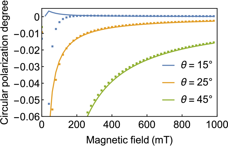
Figure 10: PL polarization degree calculated analytically after Eqs. (16) and (19) (the solid curves) and numerically after Eqs. (5) (the symbols) for the parameters $\Delta_{B}=10$ mT, $B_{ex}=\hbar|\Omega_{ex}|/(g\mu_{B})=5$ mT, $\tau_{R}=1~{}\mu$s, $\tau_{NR}=12~{}\mu$s, $\tau_{s}^{e}=15~{}\mu$s, $\tau_{s}^{h}=\tau_{1}=\tau_{2}=10^{3}~{}\mu$s, the delay time $t_{\rm d}=20~{}\mu$s. The numerical averaging was performed over 3000 hyperfine field realizations.

In Fig. 10 we demonstrate that the analytical and numerical results agree well for large magnetic fields. An increase of the magnetic field leads to the suppression of the dynamic polarization. However, the larger the tilt angle of the field, the stronger the polarization.

IV.2 Numerical results

In this section we use numeric calculations to describe the dependence of the PL intensity and polarization on time as well as magnetic field strength and orientation. We average the numeric solution of Eqs. (5) over $10^{4}$ hyperfine field realizations unless stated otherwise.

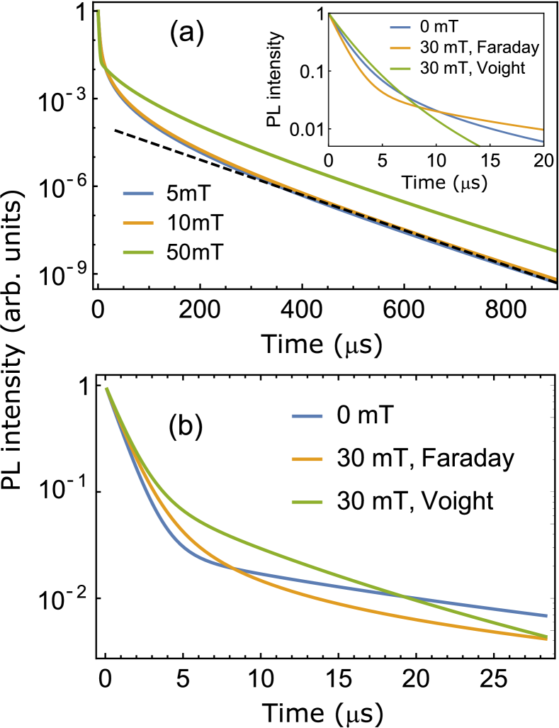
Figure 11: (a) Dynamics of the unpolarized PL calculated for different magnetic fields in Faraday geometry using the parameter $\Delta_{B}=B_{ex}=10\,{\rm mT}$. The black dashed line is proportional to $\exp(-t/72\,\mu{\rm s})$. The inset shows the unpolarized PL dynamics calculated at short time scales for zero field and a field of $30\,{\rm mT}$ in Faraday and Voigt geometry. (b) Unpolarized PL dynamics calculated using the parameters $\Delta_{B}=10\,{\rm mT}$, $B_{ex}=40\,{\rm mT}$ in Faraday and Voigt geometry at short time scales. The other parameters are given in text.

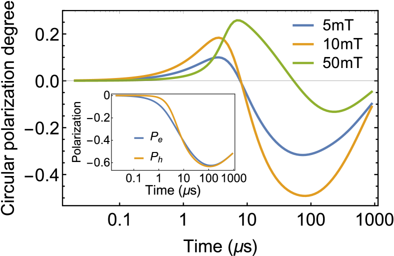
Figure 12: The dynamics of the PL polarization degree calculated for $\Delta_{B}=B_{ex}=10\,{\rm mT}$ in different magnetic fields. The inset shows the electron and hole spin polarization at $B=10\,{\rm mT}$.

We start the discussion using the following set of parameters $\Delta_{B}=B_{ex}=10\,{\rm mT}$, $\tau_{R}=1\,\mu{\rm s}$, $\tau_{NR}=100\,\mu{\rm s}$, and $\tau_{s}^{e}=\tau_{s}^{h}=\tau_{1}=\tau_{2}=1\,{\rm ms}$. In this case, the spin relaxation does not play a role. At the same time, the nonradiative recombination is slow, but it can affect the polarization at corresponding large times. We consider external magnetic fields up to 100 mT along the $z$ axis. The electron $g$ factor in indirect band gap (In,Al)As QDs was recently measured to be $g_{e}=2$ Debus ; Ivanov97 .

The dynamics of the unpolarized PL intensity (sum of $\sigma^{+}$ and $\sigma^{-}$ polarized PL components), calculated for different magnetic fields, is shown in Fig. 11(a). In a given QD it consists of four exponential contributions [see Eq. (16)], and after averaging over the hyperfine fields it becomes even more complex. However, at long delays the PL dynamics becomes almost mono-exponential. This is shown in Fig. 11(a) by the black dashed line that corresponds well to a phenomenological PL dependence on time $\propto\exp(-t/72\,\mu{\rm s})$.

The effect of the magnetic field can vary qualitatively, depending on the relation between the typical random nuclear field $\Delta_{B}$ and the exchange field $B_{\rm ex}$. In the inset of Fig. 11(a) we show that for $\Delta_{B}\gtrsim B_{\rm ex}$ the magnetic field accelerates the exciton recombination in the Voigt geometry, but decelerates it in the Faraday geometry. This is explained by the different mixing between bright and dark excitons in these two cases, which is much stronger in the Voigt than in the Faraday geometry. At the same time, in Fig. 11(b) we demonstrate that for $\Delta_{B}\ll B_{ex}$ the magnetic field can accelerate the PL decay in the Faraday geometry as well. The reason for this is the reduced splitting between bright and dark excitons for one of the heavy hole spin states.

The calculated dynamics of PL polarization in Faraday geometry is shown in Fig. 12 using the same parameters (in the Voigt geometry polarization is symmetry forbidden). The polarization is zero at $t=0$, increases up to $t\sim\tau_{R}=1\,\mu{\rm s}$, and then decreases and changes sign at $t\sim\tau_{NR}=100\,\mu{\rm s}$.

The dynamic circular polarization of the PL is induced by the external magnetic field and it is an odd function of $B_{z}$. The PL is positively polarized at short delays, and negatively polarized at long delays because the mixing between the bright and dark exciton states with $J_{z}=+3/2$ is stronger than between those with $J_{z}=-3/2$.

For the same reason the electron and hole spins in an exciton become also dynamically polarized. The electron polarization $P_{e}$ and hole polarization $P_{h}$ are defined as follows

$$P_{e}=2\frac{\braket{S_{z}^{3/2}+S_{z}^{-3/2}}}{\braket{N^{3/2}+N^{-3/2}}},$$ (20a)

$$P_{h}=\frac{\braket{N^{3/2}-N^{-3/2}}}{\braket{N^{3/2}+N^{-3/2}}}.$$ (20b)

The polarizations $P_{e}$ and $P_{h}$ are shown in the inset of Fig. 12 and behave similarly to the PL polarization, but remain always negative. At long time delays only dark excitons are left, so the polarizations of the electrons, the holes and the PL coincide.

In the absence of nonradiative recombination all excitons recombine radiatively. Since we neglect the heavy hole spin flips, the excitons with $J_{z}=\pm 3/2$ emit $\sigma^{\pm}$ polarized light, respectively. For unpolarized excitation their numbers are equal, so the integral PL is unpolarized.

The PL polarization degree calculated as a function of magnetic field for a few fixed time delays is shown in Fig. 13. One can see that it can change sign from negative to positive with increasing magnetic field strength. This can be explained as follows: The polarization is positive at short time delays and negative at long ones, as shown in Fig. 12. However, with increasing field strength in the range $B\gtrsim\Delta_{B}$ the positive part of the polarization moves to longer times. For example, for $B=10\,{\rm mT}$ the polarization changes sign at $t\approx 8\,{\rm\mu s}$, while for $B=50\,{\rm mT}$ it changes its sign at $t\approx 54\,\mu{\rm s}$. As a result, the polarization at a given time changes its sign as a function of magnetic field. For $t=20\,{\rm\mu s}$ it happens for the field $B\approx 32\,{\rm mT}$, as shown in Fig. 13.

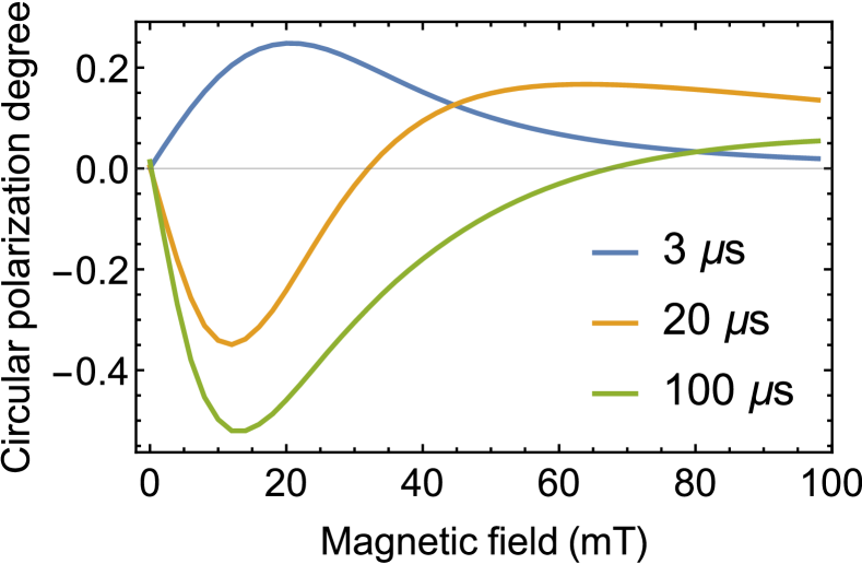
Figure 13: Magnetic field dependence of the PL polarization degree calculated for the different delay times indicated in the figure.

The influence of the various spin relaxation mechanisms is illustrated in Fig. 14, where we consider the PL polarization degree for the time delay of $20~{}\mu$s. Here, the black dashed curve reproduces the yellow curve in Fig. 13 and the other curves show the effects of the different spin relaxation times being changed from $1$ ms to $30~{}\mu$s. First, the blue curve demonstrates that a decrease of the electron spin relaxation time $\tau_{s}^{e}$ leads to suppression of the positive polarization in large fields. The red and orange curves demonstrate that decreases of the hole and of the dark exciton spin relaxation times, $\tau_{s}^{h}$ and $\tau_{2}$, respectively, have a similar effect: they lead to suppression of the negative polarization in small fields. Finally, the green curve shows that variation of the bright exciton spin relaxation time $\tau_{1}$ have almost no effect, the curve almost coincides with the black dashed one. Note, that this behaviour may change for $\tau_{1}$ shorter than $\tau_{R}$.

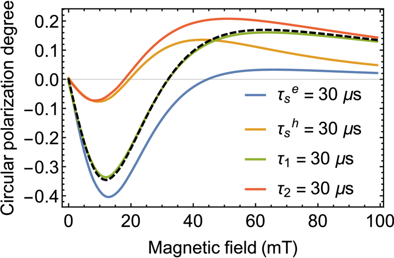
Figure 14: Magnetic field dependencies of the PL polarization degree calculated for the delay time of $20~{}\mu$s, accounting for different spin relaxation times. The black dashed curve reproduces the yellow curve from Fig. 13.

The effect of a magnetic field tilt angle is illustrated in Fig. 15. Here, the exchange field $B_{ex}=7\,{\rm mT}$ was used ($\Delta_{B}=10\,{\rm mT}$). The electron and dark exciton spin relaxations were taken to be $\tau_{s}^{e}=40\,{\rm\mu s}$ and $\tau_{2}=20\,{\rm\mu s}$. The photoluminescence was time-integrated with the parameters $t_{\rm d}=15\,{\rm\mu s}$ and $t_{\rm g}=30\,{\rm\mu s}$. One can see that at small angles the low field negative polarization is almost the same as for the pure Faraday geometry. The tilt angle flattens the positive part of the polarization. Its decrease with increasing magnetic field gets less pronounced, in agreement with the results of Sec. IV.1 and Fig. 10. The inset shows that for large tilt angles the polarization minimum shifts to larger fields and becomes deeper. Its position corresponds to $B_{z}$ of the order of $\Delta_{B}$. At the same time, the positive part of the polarization disappears. This is related to the suppression of radiative recombination of pseudo-dark excitons at $B_{z}>\Delta_{B}$. Noteworthy, a strongly tilted magnetic field can mix dark and bright excitons even without hyperfine field and lead to dynamic polarization.

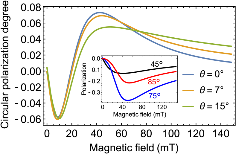
Figure 15: Magnetic field dependencies of the PL polarization degree calculated for $t_{\rm d}=15\,{\rm{\mu}s}$ and $t_{\rm g}=30\,{\rm\mu s}$ for different magnetic field tilt angles. The inset shows the same for large tilt angles indicated at the different curves.

Concluding this section, we note that the concept of dynamic electron spin polarization is similar to that of nuclear self-polarization self_nuclei and is very general. It can also take place, for example, when the electrons and holes are injected into the QDs not optically, but electrically. It is known that in organic semiconductors the hyperfine and exchange interaction lead to electron and hole spin correlations even at room temperature, which can be evidenced in magnetoresistance OMAR0 ; OMAR-ASh1 ; OMAR-ASh2 and modification of the total PL intensity OMAR-Kalin ; OMAR-Vard in small magnetic fields. Since optical orientation is very inefficient in organic semiconductors, the dynamic spin polarization may be a useful tool for spin initialization.

V Comparison between experiment and theory

The theoretical model and numerical calculated results presented in Sec. IV consider identical QDs, while in the experiment the size, shape, composition, and heterointerface smoothness strongly vary in an ensemble Shamirzaev78 ; Shamirzaev84 . However, the dynamic spin polarization requires a small exchange interaction, so the relevant electron states all belong to the $X$ valleys. As a result, the electron $g$ factor equals to $2$ in all the QDs. Moreover, since the hyperfine interaction is dominated by the contact interaction with the As nuclei Kuznetsova , the composition variations in (In,Al)As do not lead to variations of $\Delta_{B}$. Further, in experiment we detect the PL in a rather narrow window $1.66-1.70$ eV, which reduces the variance of QD sizes and, as a result, of $B_{\rm ex}$ and $\Delta_{B}$.

We expect that the strongest variations for an ensemble of (In,Al)As/AlAs QDs occur in the exciton radiative lifetimes, $\tau_{R}$. This parameter is determined mainly by the $\Gamma-X$ mixing of the electronic states at the heterointerface. The smoother the interface, the weaker the mixing Shamirzaev84 . The lifetime distribution is broad even in a given energy window Shamirzaev84 ; Rautert ; Debus ; Ivanov97 , which is evidenced by a power law decay of the PL, see Fig. 2.

It is difficult to accurately account for the spread of the QD parameters in the theory. However, the effecte of longitudinal (Faraday geometry) and transverse (Voigt geometry) magnetic fields on the dynamics of the unpolarized PL, Fig. 2, qualitatively agree with the theoretical predictions for a moderately strong exchange interaction shown in Fig. 11(b).

To describe the experiments below, we consider two sets of identical QDs. These QDs represent the cases of fast and slow radiative recombination. The QDs of the first set are described by the following parameters: $\tau_{R}=0.27\,\mu{\rm s}$, $\tau_{s}^{e}=20\,\mu{\rm s}$, $\tau_{NR}=150\,\mu{\rm s}$, $\tau_{2}=10^{3}\,\mu s$, $\tau_{s}^{h}=\tau_{1}=\tau_{NR}=\infty$, $\Delta_{B}=4.7\,{\rm mT}$, and $B_{ex}=5\,{\rm mT}$. The second set of QDs have the same parameters except for $\tau_{R}=24\,\mu{\rm s}$ and $\tau_{s}^{e}=\infty$. The number of the former QDs is $1.7$ times larger than that of the latter.

The dispersion of the exciton lifetimes is most important for the dynamics of the PL polarization shown in Fig. 5. However, it can also be qualitatively reproduced theoretically, as we demonstrate in Fig. 16(a). Here we additionally accounted for the unpolarized contribution to the PL, which decays with the time constant of $0.27~{}\mu$s. In terms of physics, this contribution can be related, for example, with the direct band gap QDs in the ensemble.

The measurement of the PL at a particular time reduces the effect of the lifetime distribution, as the QDs with the same average lifetime mostly contribute to the PL at this time. The comparison between experiment and theory is presented in Fig. 16(b), where the PL polarization degree is shown as a function of the external magnetic field for two time intervals. The overall agreement is quite good, and, in particular, the change of the sign of polarization observed in experiment is reproduced theoretically.

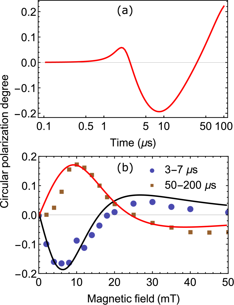
Figure 16: (a) Dynamics of the PL polarization degree calculated for an external magnetic field of $10$ mT accounting for the additional unpolarized contribution, as described in the text. (b) Comparison of experimental data (symbols) from Figs. 6(a) and 6(b) with theoretical results (lines) for the parameters given in text.

Finally, we note that some features of the polarization dependence on the magnetic field tilt angle shown in Fig. 7(a) are also captured by the theoretical model. Namely, small tilt angles hardly affect the polarization in small magnetic fields and enhance the polarization in large fields, as shown theoretically in Fig. 15. However, for a strong deviation from the Faraday geometry the experimental data shown in Fig. 7(b) are very different from the theoretical predictions shown in the inset of Fig. 15. This is a challenge for our future investigations.

VI Conclusion

The circular polarization of the PL from indirect band gap (In,Al)As/AlAs QDs has been studied experimentally in magnetic fields of different orientations up to a few hundreds of millitesla field strength, using nonresonant and unpolarized laser excitation. The polarization of PL appears as result of the dynamic electron spin polarization. We have shown that the PL polarization degree can change sign up to two times, depending on the time delay after the excitation pulse and the field strength and orientation. Most of the experimental findings have been explained using a theoretical model accounting for the electron-hole exchange interaction and the hyperfine interaction. The dispersion of the QD parameters plays a significant role in the calculation of the PL polarization degree, open questions still remain with respect to the experimental results in magnetic fields strongly tilted from the structure growth axis.

Acknowledgements. We thank M. M. Glazov and M. O. Nestoklon for fruitful discussions. The experimental part of this research has been supported by the Deutsche Forschungsgemeinschaft (Grant No. 409810106) and by the Russian Foundation for Basic Research (Grants Nos. 19-52-12001 and 19-02-00098). M.B. acknowledges the support by the Deutsche Forschungsgemeinschaft (ICRC TRR 160, project A01). The theoretical studies by D.S.S. were supported by the RF President Grant No. MK-5158.2021.1.2, the Foundation for the Advancement of Theoretical Physics and Mathematics “BASIS”, and the Russian Foundation for Basic Research Grants Nos. 19-52-12054 and 20-32-70048. The theoretical studies by A.V.S. were supported by the Russian Foundation for Basic Research Grant No. 19-02-00184.

References

- (1)
- (2) Spin Physics in Semiconductors, ed. M. I. Dyakonov (Springer, Berlin, 2008).
- (3) M. M. Glazov, Electron and Nuclear Spin Dynamics in Semiconductor Nanostructures (Oxford University Press, Oxford, UK, 2018).
- (4) M. I. Dyakonov, Will We Ever Have a Quantum Computer? (Springer International Publishing, Berlin, Germany, 2020).
- (5) A. Fert, The origin, development and future of spintronics, Phys. Usp. 51, 1336 (2008).
- (6) Optical Orientation, eds. F. Meier and B. P. Zakharchenja (North-Holland, Amsterdam, 1984).
- (7) P. Zeeman, The effect of magnetisation on the nature of light emitted by a substance, Nature 55, 347 (1897).
- (8) T. S. Shamirzaev, Exciton recombination and spin dynamics in indirect-gap quantum wells and quantum dots, Phys. Solid State 60, 1554 (2018).
- (9) T. S. Shamirzaev, J. Rautert, D. R. Yakovlev, J. Debus, A. Yu. Gornov, M. M. Glazov, E. L. Ivchenko, and M. Bayer, Spin dynamics and magnetic field induced polarization of excitons in ultrathin GaAs/AlAs quantum wells with indirect band gap and type-II band alignment, Phys. Rev. B 96, 035302 (2017).
- (10) T. S. Shamirzaev, J. Debus, D. R. Yakovlev, M. M. Glazov, E. L. Ivchenko, and M. Bayer, Dynamics of exciton recombination in strong magnetic fields in ultrathin GaAs/AlAs quantum wells with indirect band gap and type-II band alignment, Phys. Rev. B 94, 045411 (2016).
- (11) E. L. Ivchenko, Magnetic circular polarization of exciton photoluminescence, Phys. Solid State 60, 1514 (2018).
- (12) D. S. Smirnov, T. S. Shamirzaev, D. R. Yakovlev, and M. Bayer, Dynamic Polarization of Electron Spins Interacting with Nuclei in Semiconductor Nanostructures, Phys. Rev. Lett. 125, 156801 (2020).
- (13) T. S. Shamirzaev, A. V. Nenashev, A. K. Gutakovskii, A. K. Kalagin, K. S. Zhuravlev, M. Larsson, and P. O. Holtz, Atomic and energy structure of InAs/AlAs quantum dots, Phys. Rev. B 78, 085323 (2008).
- (14) T. S. Shamirzaev, D. S. Abramkin, D. V. Dmitriev, and A. K. Gutakovskii, Nonradiative energy transfer between vertically coupled indirect and direct bandgap InAs quantum dots, Appl. Phys. Lett. 97, 263102 (2010).
- (15) T. S. Shamirzaev, A. M. Gilinsky, A. K. Kalagin, A. I. Toropov, A. K. Gutakovskii and K. S. Zhuravlev, Strong sensitivity of photoluminescence of InAs/AlAs quantum dots to defects: evidence for lateral inter-dot transport, Semicond. Sci. Technol. 21, 527 (2006).
- (16) I. Vurgaftman, J. R. Meyer, and L. R. Ram-Mohan, Band parameters for III-V compound semiconductors and their alloys, J. Appl. Phys. 89, 5815 (2001)
- (17) T. S. Shamirzaev, J. Debus, D. S. Abramkin, D. Dunker, D. R. Yakovlev, D. V. Dmitriev, A. K. Gutakovskii, L. S. Braginsky, K. S. Zhuravlev, and M. Bayer, Exciton recombination dynamics in an ensemble of (In,Al)As/AlAs quantum dots with indirect band-gap and type-I band alignment, Phys. Rev. B 84, 155318 (2011).
- (18) D. Keller, D. R. Yakovlev, B. König, W. Ossau, Th. Gruber, A. Waag, L. W. Molenkamp, and A. V. Scherbakov, Heating of the magnetic ion system in (Zn,Mn)Se/(Zn,Be)Se semimagnetic quantum wells by means of photoexcitation, Phys. Rev. B 65, 035313 (2002).
- (19) T. S. Shamirzaev, A. V. Nenashev, and K. S. Zhuravlev, Coexistence of direct and indirect band structures in arrays of InAs/AlAs quantum dots, Appl. Phys. Lett. 92, 213101 (2008).
- (20) The preliminary empirical tight binding calculations suggest that for small QDs the electron ground state might belong to the valley and be localized at the apex of the QDs Nestoklon similarly to (In,Ga)As/GaP QDs Cedric1 ; Cedric2 .
- (21) M. O. Nestoklon, private communication.
- (22) C. Robert, M. O. Nestoklon, K. Pereira da Silva, L. Pedesseau, C. Cornet, M. I. Alonso, A. R. Goñi, P. Turban, J.-M. Jancu, J. Even, and O. Durand, Strain-induced fundamental optical transition in (In,Ga)As/GaP quantum dots, Appl. Phys. Lett. 104, 011908 (2014).
- (23) C. Robert, K. Pereira Da Silva, M. O. Nestoklon, M. I. Alonso, P. Turban, J.-M. Jancu, J. Even, H. Carrère, A. Balocchi, P. M. Koenraad, X. Marie, O. Durand, A. R. Goñi, and C. Cornet, Electronic wave functions and optical transitions in (In,Ga)As/GaP quantum dots, Phys. Rev. B 94, 075445 (2016).
- (24) T. S. Shamirzaev, Type-I semiconductor heterostructures with an indirect gap conduction band, Semiconductors 45, 96 (2011).
- (25) M. E. Pistol, and C. E. Pryor, Band structure of segmented semiconductor nanowires, Phys. Rev. B 80, 035316 (2009).
- (26) D. S. Abramkin and T. S. Shamirzaev, Type-I indirect-gap semiconductor heterostructures on (110) substrates, Semiconductors 53, 703 (2019).
- (27) T. S. Shamirzaev, D. S. Abramkin, A. K. Gutakovskii, and M. A. Putyato, High quality relaxed GaAs quantum dots in GaP matrix, Appl. Phys. Lett. 97, 023108 (2010).
- (28) J. Rautert, M. V. Rakhlin, K. G. Belyaev, T. S. Shamirzaev, A. K. Bakarov, A. A. Toropov, I. S. Mukhin, D. R. Yakovlev, and M. Bayer, Anisotropic exchange splitting of excitons affected by -X mixing in (In,Al)As/AlAs quantum dots: Microphotoluminescence and macrophotoluminescence measurements, Phys. Rev. B 100, 205303 (2019).
- (29) T. S. Shamirzaev, D. S. Abramkin, A. V. Nenashev, K. S. Zhuravlev, F. Trojanek, B. Dzurnak, and P. Maly, Carrier dynamics in InAs/AlAs quantum dots: lack in carrier transfer from wetting layer to quantum dots, Nanotechnology 21, 155703 (2010).
- (30) E. L. Ivchenko, Optical Spectroscopy of Semiconductor Nanostructures (Alpha Science, Harrow, UK, 2005).
- (31) G. V. Astakhov, A. V. Koudinov, K. V. Kavokin, I. S. Gagis, Yu. G. Kusrayev, W. Ossau, and L. W. Molenkamp, Exciton Spin Decay Modified by Strong Electron-Hole Exchange Interaction, Phys. Rev. Lett. 99, 016601 (2007).
- (32) G. L. Bir and G. E. Pikus, Symmetry and Deformational Effects in Semiconductors (Wiley, New York, 1974).
- (33) S. V. Goupalov, P. Lavallard, G. Lamouche, and D. S. Citrin, Electrodynamical treatment of the electron-hole long-range exchange interaction in semiconductor nanocrystals, Phys. Solid State 45, 768 (2003).
- (34) M. S. Kuznetsova, J. Rautert, K. V. Kavokin, D. S. Smirnov, D. R. Yakovlev, A. K. Bakarov, A. K. Gutakovskii, T. S. Shamirzaev, and M. Bayer, Electron-nuclei interaction in the valley of (In,Al)As/AlAs quantum dots, Phys. Rev. B 101, 075412 (2020).
- (35) X. Marie, T. Amand, P. Le Jeune, M. Paillard, P. Renucci, L. E. Golub, V. D. Dymnikov, and E. L. Ivchenko, Hole spin quantum beats in quantum-well structures, Phys. Rev. B 60, 5811 (1999).
- (36) J. Debus, T. S. Shamirzaev, D. Dunker, V. F. Sapega, E. L. Ivchenko, D. R. Yakovlev, A. I. Toropov, and M. Bayer, Spin-flip Raman scattering of the -X mixed exciton in indirect band gap (In,Al)As/AlAs quantum dots, Phys. Rev. B 90, 125431 (2014).
- (37) E. A. Chekhovich, M. M. Glazov, A. B. Krysa, M. Hopkinson, P. Senellart, A. Lemaitre, M. S. Skolnick, and A. I. Tartakovskii, Element-sensitive measurement of the hole-nuclear spin interaction in quantum dots, Nat. Phys. 9, 74 (2013).
- (38) I. D. Avdeev and D. S. Smirnov, Hyperfine interaction in atomically thin transition metal dichalcogenides, Nanoscale Adv. 1, 2624 (2019).
- (39) V. L. Korenev, Dynamic self-polarization of nuclei in low-dimensional systems, JETP Lett. 70, 129 (1999).
- (40) M. Y. Petrov, G. G. Kozlov, I. V. Ignatiev, R. V. Cherbunin, D. R. Yakovlev, and M. Bayer, Solvable quantum model of dynamic nuclear polarization in optically driven quantum dots, Phys. Rev. B 80, 125318 (2009).
- (41) E. A. Zhukov, E. Kirstein, D. S. Smirnov, D. R. Yakovlev, M. M. Glazov, D. Reuter, A. D. Wieck, M. Bayer, and A. Greilich, Spin inertia of resident and photoexcited carriers in singly charged quantum dots, Phys. Rev. B 98, 121304(R) (2018).
- (42) A. V. Shumilin and D. S. Smirnov, Nuclear Spin Dynamics, Noise, Squeezing, and Entanglement in Box Model, Phys. Rev. Lett. 126, 216804 (2021).
- (43) A. V. Shchepetilnikov, D. D. Frolov, Yu. A. Nefyodov, I. V. Kukushkin, D. S. Smirnov, L. Tiemann, C. Reichl, W. Dietsche, and W. Wegscheider, Nuclear magnetic resonance and nuclear spin relaxation in AlAs quantum well probed by ESR, Phys. Rev. B 94, 241302(R) (2016).
- (44) I. A. Merkulov, Al. L. Efros, and M. Rosen, Electron spin relaxation by nuclei in semiconductor quantum dots, Phys. Rev. B 65, 205309 (2002).
- (45) D. S. Smirnov, E. A. Zhukov, D. R. Yakovlev, E. Kirstein, M. Bayer, and A. Greilich, Spin polarization recovery and Hanle effect for charge carriers interacting with nuclear spins in semiconductors, Phys. Rev. B 102, 235413 (2020).
- (46) These notations are related to the notations of Ref. Smirnov125 as follows: , .
- (47) V. Yu. Ivanov, T. S. Shamirzaev, D. R. Yakovlev, A. K. Gutakovskii, Ł. Owczarczyk, and M. Bayer, Optically detected magnetic resonance of photoexcited electrons in (In,Al)As/AlAs quantum dots with indirect band gap and type-I band alignment, Phys. Rev. B 97, 245306 (2018).
- (48) M. I. Dyakonov and V. I. Perel, Dynamic nuclear self-polarization, Pis’ma Zh. Exsp. Teor. Fiz. 16, 563 (1972) [JETP Lett. 16, 398 (1972)].
- (49) O. Mermer, G. Veeraraghavan, T. L. Francis, Y. Sheng, D. T. Nguyen, M. Wohlgenannt, A. Kohler, M. K. Al-Suti, and M. S. Khan, Large magnetoresistance in nonmagnetic -conjugated semiconductor thin film devices, Phys. Rev. B 72, 205202 (2005).
- (50) A. V. Shumilin, V. V. Kabanov, and V. I. Dediu, Magnetoresistance in organic semiconductors: Including pair correlations in the kinetic equations for hopping transport, Phys. Rev. B 97, 094201 (2018).
- (51) A. V. Shumilin, Microscopic theory of organic magnetoresistance based on kinetic equations for quantum spin correlations, Phys. Rev. B 101, 134201 (2020).
- (52) J. Kalinowski, M. Cocchi, D. Virgili, P. Di Marco, and V. Fattori, Magnetic field effects on emission and current in Alq3-based electroluminescent diodes, Chem. Phys. Lett. 380, 710 (2003).
- (53) T. D. Nguyen, G. Hukic-Markosian, F. Wang, L. Wojcik, X.-G. Li, E. Ehrenfreund, and Z. V. Vardeny, Isotope effect in spin response of -conjugated polymer films and devices, Nat. Mater. 9, 345 (2010).
- (54) J. Rautert, T. S. Shamirzaev, S. V. Nekrasov, D. R. Yakovlev, P. Klenovský, Yu. G. Kusrayev, and M. Bayer, Optical orientation and alignment of excitons in direct and indirect band gap (In,Al)As/AlAs quantum dots with type-I band alignment, Phys. Rev. B 99, 195411 (2019).
- (55) M. Dyakonov, X. Marie, T. Amand, P. Le Jeune, D. Robart, M. Brousseau, and J. Barrau, Coherent spin dynamics of excitons in quantum wells, Phys. Rev. B 56, 10412 (1997).