Gravitational waves from first-order phase transitions in Majoron models of neutrino mass

Abstract

We show how the generation of right-handed neutrino masses in Majoron models may be associated with a first-order phase transition and accompanied by the production of a stochastic background of gravitational waves (GWs). We explore different energy scales with only renormalizable operators in the effective potential. If the phase transition occurs above the electroweak scale, the signal can be tested by future interferometers. We consider two possible energy scales for phase transitions below the electroweak scale. If the phase transition occurs at a GeV, the signal can be tested at LISA and provide a complementary cosmological probe to right-handed neutrino searches at the FASER detector. If the phase transition occurs below 100 keV, we find that the peak of the GW spectrum is two or more orders of magnitude below the putative NANOGrav GW signal at low frequencies, but well within reach of the SKA and THEIA experiments. We show how searches of very low frequency GWs are motivated by solutions to the Hubble tension in which ordinary neutrinos interact with the dark sector. We also present general calculations of the phase transition temperature and Euclidean action that apply beyond Majoron models.

1 Introduction

The recent discovery of GWs provides a powerful phenomenological tool to probe the imprint of new physics in the early universe. Primordial GWs that survive until the present could have been produced by mechanisms that rely on new physics. In particular, strong first-order phase transitions are a well known source of gravitational radiation Witten:1984rs ; Hogan:1986qda ; Turner:1990rc that could be detectable in the form of a stochastic GW background. These have been studied within the standard model (SM), either in relation to a QCD phase transition Witten:1984rs or to an electroweak phase transition Kamionkowski:1993fg . However, it is now established that both electroweak symmetry breaking and the approximate QCD chiral symmetry breaking occur as a smooth crossover, with no phase transition, so that no associated stochastic GW background is predicted within the SM. Still, the necessity to extend the SM to explain outstanding cosmological puzzles and to incorporate neutrino masses and mixing, motivates the study of first-order phase transitions in the early universe. In this way primordial GWs are an important tool, complementary to more traditional ones, to probe physics beyond the SM. For example, GW production from a strong first-order phase transition in the early universe has been studied jointly with electroweak baryogenesis within supersymmetric models Apreda:2001us , or in association with dark matter genesis Witten:1984rs ; Bai:2018dxf , or both Huang:2017kzu ; Hall:2019rld , and even with the simultaneous genesis of dark matter and neutrino masses DiBari:2020bvn .

In this paper we explore first-order phase transitions within extensions of the SM that can explain neutrino masses and mixing. In this respect, the type-I seesaw mechanism offers an attractive way to explain neutrino masses with the addition of right-handed (RH) neutrinos with large Majorana masses. In this case the generation of heavy neutrino Majorana masses can provide a natural framework for the realization of a first-order phase transition in the early universe. In particular, the Majoron model Chikashige:1980ui provides a way to embed the type-I seesaw mechanism and at the same time to generate Majorana masses. This is done through the introduction of a complex scalar field with terms in the Lagrangian respecting $U(1)_{L}$ symmetry spontaneously broken below a critical temperature. Since spontaneous symmetry breaking can occur via a strong first-order phase transition, an associated production of GWs is possible, in a way that GW experiments can probe the origin of Majorana masses and give insight on the scale of symmetry breaking. The scale of symmetry breaking is not predicted by the model. It is useful to distinguish high scale scenarios, in which the scale is above the electroweak scale, from low scale scenarios, in which the scale is below the electroweak scale. In the latter case, it is intriguing that the pulsar timing array experiment NANOGrav has recently found strong evidence for a stochastic GW background in the frequency band $\sim 10^{-8}$ Hz in the 12.5-year dataset Arzoumanian:2020vkk . In our scenario, the phase transition occurs in the dark sector which includes the complex scalar and RH neutrinos. The dark sector interacts with the SM sector gravitationally and with nonstandard interactions. The possibility that a low scale dark phase transition may address the NANOGrav result has been recently considered in Ref. Nakai:2020oit (see also Bian:2021lmz for a Bayesian analysis comparing it with other explanations) and, more specifically, within a Majoron model with nonrenormalizable effective operators in Ref. Addazi:2020zcj . A general discussion on GW production from a first-order phase transition in dark sectors has been presented in Refs. Breitbach:2018ddu ; Fairbairn:2019xog . In our paper we consider a few scenarios with only renormalizable terms in the tree level potential and including one-loop zero and finite temperature contributions. For each model we calculate the GW spectrum and compare it to the sensitivity of existing and planned experiments.

The paper is organized as follows. In Section 2, we discuss the form of the effective potential within different scenarios. In particular, we discuss both the tree-level and the one-loop, zero temperature and finite temperature contributions to the effective potential in the high scale case. In Section 3, we discuss the first-order phase transition and the associated GW production for high scale scenarios. We scan over the parameter space (at or above the electroweak scale) and show that some of the models can be tested at future gravitational interferometers. In Section 4 we consider low energy scale scenarios, well below the electroweak scale. In particular, we attempt to reproduce the NANOGrav signal and also make connection with the Hubble tension in the $\Lambda$CDM model . Finally, in Section 5, we highlight some points and draw our conclusions.

2 Effective potential in Majoron models

The Majoron model is a simple extension of the SM Chikashige:1980ui . Spontaneous breaking of a global $U_{L}(1)$ symmetry generates a Majorana mass term for the RH neutrinos, which in combination with a Dirac mass term, generates the light neutrino masses via the type-I seesaw mechanism. To implement this, the SM field content is augmented with $N\geq 2$ RH neutrinos $N_{I}$, and a complex scalar singlet,

$$\sigma={1\over\sqrt{2}}\,(\sigma_{1}+i\,\sigma_{2})\,,$$ (1)

where the real component is CP-even and the imaginary component is CP-odd. The new scalar $\sigma$ has a tree level potential $V_{0}(\sigma)$. Then, the tree-level extension of the SM Lagrangian is

$$-{\cal L}_{N_{I}+\sigma} = \overline{L_{\alpha}}\,h_{\alpha I}\,N_{I}\,\widetilde{\Phi}+{\lambda_{I}\over 2}\,\sigma\,\overline{N_{I}^{c}}\,N_{I}+V_{0}(\sigma)+{\rm h.c.}\,,$$ (2)

where $\widetilde{\Phi}$ is the dual Higgs doublet. As we will discuss, above a critical temperature $T_{\rm c}$, $\langle\sigma\rangle=0$ and the RH neutrinos are massless. Since the lepton doublets $L_{\alpha}$ and RH neutrinos $N_{I}$ have $L=1$, and $\sigma$ has $L=2$, lepton number is conserved. Below $T_{\rm c}$, the $U_{L}(1)$ symmetry is broken, the scalar $\sigma$ gets a vacuum expectation value $\langle\sigma\rangle=v/\sqrt{2}$ and the RH neutrinos gain Majorana masses $M_{I}=v\,\lambda_{I}/\sqrt{2}$, which leads to lepton number violation and small masses for the SM Majorana neutrinos via the type-I seesaw mechanism. We assume in this and next section that $T_{\rm c}\gtrsim T_{\rm ew}\sim 100\,{\rm GeV}$, so that the Majorana mass term is not generated later than the Dirac mass term.

2.1 Minimal model

Consider the form of the tree-level potential $V_{0}(\sigma)$. We neglect a possible contribution from the mixing of the new scalar with the standard Higgs boson. Imposing a global $U(1)_{L}$ symmetry and keeping only renormalizable terms, the tree level potential can be simply written as

$$V_{0}(\sigma)=-\mu^{2}|\sigma|^{2}+\lambda|\sigma|^{4}\,.$$ (3)

Here, $\lambda$ is real and positive, so that the potential is bounded from below, and $\mu^{2}$ is real and positive to ensure the existence of degenerate nontrivial stable minima with $\langle\sigma\rangle=v_{0}\,e^{i\theta}/\sqrt{2}$ ($0\leq\theta<2\pi$), where $v_{0}\equiv\sqrt{\mu^{2}/\lambda}$. In the broken phase we can rewrite $\sigma$ as

$$\sigma={e^{i\theta}\over\sqrt{2}}\,(v_{0}+S+i\,J)\,,$$ (4)

where $S$ is a massive field with $m_{S}^{2}=2\lambda v_{0}^{2}$ and $J$ is the Majoron, a massless Goldstone field. The vacuum expectation value of $\sigma$ also generates RH neutrino masses $M_{I}=\lambda_{I}\,v_{0}/\sqrt{2}$ and these, via the type-I seesaw mechanism, lead to a light neutrino mass matrix given by the seesaw formula,

$$(m_{\nu})_{\alpha\beta}=-{v_{\rm ew}^{2}\over 2}{h_{\alpha I}h_{\beta I}\over M_{I}}\,,$$ (5)

where $v_{\rm ew}$ is the standard Higgs vacuum expectation value. Equation (5) is understood to be in the flavor basis in which the charged lepton and Majorana mass matrices are diagonal.

The tree-level zero-temperature potential $V_{0}(\sigma)$ describes the broken symmetry phase of the dark sector that includes the scalar field $\sigma$ and the RH neutrinos. The dark sector couples to the thermal bath of SM particles via the Yukawa interactions of the $N_{I}$’s. In particular, $2\rightarrow 2$ scatterings (such as $L+q\rightarrow N_{I}+t$) can thermalize the RH neutrinos even if they are massless. Indeed, the abundance of the ultrarelativistic RH neutrino $N_{I}$, normalized so that $N_{N_{I}}^{\rm eq}=1$, evolves simply as $N_{N_{I}}=1-\exp[-T^{\rm eq}_{I}/T]$, where $T^{\rm eq}_{I}$ is the $N_{I}$ equilibration temperature given by Garbrecht:2013bia ; DiBari:2019zcc

$$T^{\rm eq}_{I}\simeq 0.2\,{(h^{\dagger}\,h)_{II}\,v_{\rm ew}^{2}\over m_{\rm eq}}=0.2\,M_{I}\,K_{I}\,,$$ (6)

where $m_{\rm eq}=[16\pi^{5/2}\sqrt{g^{\star}_{\rho}}/(3\sqrt{5})]\,(v_{\rm eq}/M_{\rm P})\simeq 1.1\,{\rm meV}\,\sqrt{g^{\star}_{\rho}/g^{\rm SM}_{\rho}}$ is the usual effective equilibrium neutrino mass, and $K_{I}\equiv(h^{\dagger}\,h)_{II}\,v_{\rm ew}^{2}/(M_{I}\,m_{\rm eq})$ is the usual RH neutrino decay parameter. Here, $g_{\rho}^{\star}\equiv g_{\rho}(t_{\star})$ is the number of ultrarelativistic degrees of freedom at the time of the phase transition $t_{\star}$, which in the cases of interest to us, is just after the time of RH neutrino production. In the standard case, when the dynamics occurs above the electroweak scale, this can be well approximated by the SM number of degrees of freedom. More accurately, one should include the small contribution from the RH neutrinos and the complex scalar, but this level of accuracy is not needed at this stage.

For $M_{I}/T_{\rm c}\gtrsim 5/K_{I}$, the RH neutrino $N_{I}$ reaches thermal equilibrium before the onset of the phase transition, and is unable to decay prior to this because it is massless. In order for the seesaw formula to be consistent with neutrino oscillation data without fine-tuning, at least two decay parameters must be in the range $10$–$100$. Only a possible third RH neutrino can have an arbitrarily small $K_{I}$. For definiteness, when studying high scale scenarios, we assume that all three RH neutrinos have decay parameters and masses that satisfy $K_{I}\,M_{I}\gtrsim 5\,T_{\rm c}$, so that they are all in thermal equilibrium prior to the onset of the phase transition.

In addition, the $N_{I}$’s couple to the scalar field through $N_{I}+N_{I}\leftrightarrow\sigma$. In this case, the interaction rate is $\Gamma_{\sigma}\sim(M_{I}/v_{0})^{2}\,T$ and the processes can be assumed to be in equilibrium (i.e., $\Gamma_{\sigma}>H$) at the time of the phase transition for a reasonable choice of parameters. In the following we assume that the dark sector is in thermal equilibrium with the SM sector prior to the phase transition.

Finite temperature effects induce symmetry restoration at temperatures above the critical temperature Kirzhnits:1972ut and govern the dynamics responsible for the phase transition from the metastable vacuum (where lepton number is conserved and neutrinos are massless), to the true vacuum (where lepton number is violated and neutrinos acquire masses). These effects are well described by the one-loop effective potential at finite temperatures $V^{T}_{1}(\sigma)$. The one-loop contribution also generates a zero-temperature term $V^{0}_{1}(\sigma)$ that needs to be included for consistency. Then, the finite-temperature effective potential at one-loop is Dolan:1973qd

$$V_{\rm eff}^{T}(\sigma)=V_{0}(\sigma)+V^{0}_{1}(\sigma)+V^{T}_{1}(\sigma)\,.$$ (7)

The zero temperature one-loop contribution is given by the Coleman-Weinberg potential that can be written, using cut-off regularization, as Dolan:1973qd ; Anderson:1991zb ; Dine:1992wr ; Quiros:1999jp

$$V^{0}_{1}(\sigma) = {1\over 64\,\pi^{2}}\,\left\{m_{\sigma}^{4}(\sigma)\,\left(\log{m^{2}_{\sigma}(\sigma)\over m^{2}_{\sigma}(v_{0})}-{3\over 2}\right)+2\,m_{\sigma}^{2}(\sigma)\,m^{2}_{\sigma}(v_{0})\right.$$

$$\left.\;\;\;\;\;\;\;-2\,\sum_{I}\,\left[M_{I}^{4}(\sigma)\,\left(\log{M_{I}^{2}(\sigma)\over M^{2}_{I}(v_{0})}-{3\over 2}\right)+2\,M^{2}_{I}(\sigma)\,M_{I}^{2}(v_{0})\right]\right\}\,,$$

where the prefactor of two in the second line accounts for the two degrees of freedom for each of the three RH neutrinos. The one-loop thermal potential is given by Anderson:1991zb ; Dine:1992wr ; Quiros:1999jp

$$V^{T}_{1}(\sigma)=\frac{T^{4}}{2\pi^{2}}\left[J_{B}\left(\frac{m_{\sigma}^{2}(\sigma)}{T^{2}}\right)-2\sum_{I}J_{F}\left(\frac{M_{I}^{2}(\sigma)}{T^{2}}\right)\right]\,,$$ (9)

where the thermal functions are

$$J_{B,F}(x^{2})=\int_{0}^{\infty}dy\,y^{2}\,\log(1\mp e^{-\sqrt{x^{2}+y^{2}}})\,,$$ (10)

and $m_{\sigma}^{2}(\sigma)$ and $M_{I}^{2}(\sigma)$ are the shifted masses. Without loss of generality, we set $\theta=0$ in Eq. (4) so that the minimum of the potential including thermal effects, lies along the real axis of $\sigma$. In this way we can track the dynamics of the potential as a function of $\sigma_{1}$. The tree-level potential becomes

$$V_{0}(\sigma_{1})=-{1\over 2}\,\mu^{2}\,\sigma_{1}^{2}+{\lambda\over 4}\,\sigma_{1}^{4}\,,$$ (11)

and the shifted masses are

$$m_{\sigma}^{2}(\sigma_{1})\equiv{d^{2}V^{0}(\sigma_{1})\over d^{2}\sigma_{1}}=-\lambda v_{0}^{2}+3\lambda\sigma_{1}^{2}$$ (12)

and

$$M_{I}^{2}(\sigma_{1})=\lambda_{I}^{2}\,{\sigma_{1}^{2}\over 2}\,.$$ (13)

Note that $m_{\sigma}^{2}(\sigma_{1})$ can be either positive or negative, depending on the size of $\sigma_{1}$. An imaginary part of the effective potential is obtained for $m_{\sigma}^{2}(\sigma_{1})<0$. This corresponds to decay widths of modes expanded around unstable regions of field space and does not affect the computation of the phase transition Delaunay:2007wb . Therefore, in the following we neglect the imaginary part of the potential. We account for resummed thermal masses by replacing the tree-level shifted mass in Eq. (9) by Parwani:1991gq

$$m_{\sigma}^{2}(\sigma_{1})\to{\rm m}_{\sigma,T}^{2}(\sigma_{1})=m_{\sigma}^{2}(\sigma_{1})+\Pi_{\sigma}\,.$$ (14)

The leading contribution to the thermal mass, i.e., the Debye mass, is given by

$$\Pi_{\sigma}=\left(\frac{2+d_{\rm scalar}}{12}\lambda+N\,\frac{M^{2}}{24v_{0}^{2}}\right)T^{2}\,,$$ (15)

where $d_{\rm scalar}=2$ for a complex scalar. This yields the so-called dressed effective potential Curtin:2016urg ; Croon:2020cgk . $M$ denotes either the mass of the heaviest RH neutrino, if it gives the dominant contribution (in which case $N=1$), or a common mass for quasi-degenerate RH neutrinos (in which case $N$ is the number of RH neutrinos). This allows us to reduce the number of parameters while spanning the space between $N=1$ (hierarchical RH neutrinos) and $N=3$ (quasi-degenerate RH neutrinos).

It is useful to write the effective potential in terms of the high temperature expansion of the thermal functions Anderson:1991zb ; Quiros:1999jp ,

$$J_{B}(x^{2}) = -\frac{\pi^{4}}{45}+\frac{\pi^{2}x^{2}}{12}-\frac{\pi}{6}(x^{2})^{3/2}-\frac{x^{4}}{32}\,\log{x^{2}\over a_{B}}+{\cal O}(x^{6})\,,$$

$$J_{F}(x^{2}) = \frac{7\pi^{4}}{360}-\frac{\pi^{2}x^{2}}{24}-\frac{x^{4}}{32}\,\log{x^{2}\over a_{F}}+{\cal O}(x^{6})\,,$$ (16)

where $a_{B}=16\,\pi^{2}\,\exp(3/2-2\gamma_{E})$ and $a_{F}=\pi^{2}\exp(3/2-2\gamma_{E})$, with $\gamma_{E}=0.5772$. We checked that this expansion is accurate to better than $\sim 5\%,12\%,27\%$ for $x^{2}\leq 3,4,5$, respectively. In our numerical work, we set $x^{2}\leq 3$.

Since we are assuming that the RH neutrinos are thermalized, the field dependence in the logarithmic term in Eq. (2.1) cancels the logarithmic term in the high temperature expansion of $V^{T}_{1}(\sigma)$ to leave the one-loop finite-temperature effective potential in a polynomial form,

$$V^{T}_{\rm eff}(\sigma_{1})\simeq D\,(T^{2}-T_{0}^{2})\sigma_{1}^{2}-A\,T\,\sigma_{1}^{3}+\frac{1}{4}\lambda_{T}\,\sigma_{1}^{4}\,,$$ (17)

where the destabilization temperature $T_{0}$ is defined by

$$2\,D\,T_{0}^{2}=\lambda\,v_{0}^{2}+{N\over 8\,\pi^{2}}\,{M^{4}\over v_{0}^{2}}-{3\over 8\,\pi^{2}}\lambda^{2}\,v_{0}^{2}\,,$$ (18)

and the dimensionless coefficients $D$ and $A$ are

$$D={{\lambda\over 8}+{N\over 24}\,{M^{2}\over v_{0}^{2}}}\,\;\;\;\;\mbox{\rm and}\;\;\;\;A={(3\,\lambda)^{3/2}\over 12\pi}\,\,.$$ (19)

The cubic term is obtained using the approximation, $m^{2}_{\sigma}(\sigma_{1})=\Pi_{\sigma}-\lambda v_{0}^{2}+3\lambda\sigma_{1}^{2}\simeq 3\lambda\sigma_{1}^{2}$. This approximation works quite well since the cubic term gives a nonnegligible contribution only when the field is large. The dimensionless temperature dependent coefficient $\lambda_{T}$ is given by

$$\lambda_{T}=\lambda-\frac{N\,M^{4}}{8\,\pi^{2}\,v_{0}^{4}}\,\log{a_{F}\,T^{2}\over e^{3/2}\,M^{2}}+{9\lambda^{2}\over 16\pi^{2}}\,\log{a_{B}\,T^{2}\over e^{3/2}\,m_{S}^{2}}\,.$$ (20)

In the following it will prove convenient to define

$$\widetilde{M}_{T}^{2}\equiv 2\,D\,(T^{2}-T_{0}^{2})\,,$$ (21)

so that the thermal effective potential can be written more compactly as

$$V^{T}_{\rm eff}(\sigma_{1})\simeq{1\over 2}\,\widetilde{M}_{T}^{2}\,\sigma_{1}^{2}-A\,T\,\sigma_{1}^{3}+\frac{1}{4}\lambda_{T}\,\sigma_{1}^{4}\,.$$ (22)

Finally, note that the massive scalar $S$ must decay for its thermal abundance not to overclose the universe. Since the scalar and RH neutrino masses are of roughly the same order-of-magnitude as $v_{0}$, we can always assume that the mass of the lightest RH neutrino $M_{1}<m_{S}$ and that $S$ decays quickly enough via $S\rightarrow N_{1}+N_{1}$.

2.2 Explicit symmetry breaking term and a massive Majoron

It might be useful for various applications to give the Majoron a mass. This can be done by adding an explicit symmetry breaking term $V_{L\!\!\!/}(\sigma)$ to the tree-level potential, obtaining

$$V_{0}(\sigma)=-\mu^{2}|\sigma|^{2}+\lambda|\sigma|^{4}+V_{L\!\!\!/}(\sigma)\,.$$ (23)

Consider the $U(1)_{L}$-breaking renormalizable term,

$$V_{L\!\!\!/}(\sigma)=-\sqrt{2}\,\widetilde{m}\,\sigma^{2}\sigma^{*}+{\rm h.c.}\,,$$ (24)

where the mass-dimension parameter $\widetilde{m}$ can always be taken to be real by absorbing a phase into $\sigma$. Other renormalizable terms that break $U(1)_{L}$ explicitly are proportional to $\sigma^{2}$, $\sigma^{3}$, $\sigma^{4}$ and $\sigma^{3}\sigma^{*}$ and their complex conjugates. However, these terms are invariant under a discrete symmetry, either $Z_{2}$, $Z_{3}$ or $Z_{4}$, and the spontaneous breaking of a discrete symmetry may induce a domain wall problem Vilenkin:1984ib ; Kibble:1976sj . For this reason we assume $V_{L\!\!\!/}$ in Eq. (24) to be the only explicit breaking term. Its inclusion breaks the degeneracy of the minima with only one minimum located on the real axis at $\theta=0$ for $\widetilde{m}>0$, and with a vacuum expectation value,

$$v_{0}(\widetilde{m})=\sqrt{\frac{\mu^{2}}{\lambda}+\left(\frac{3\,\widetilde{m}}{2\lambda}\right)^{2}}+\frac{3\,\widetilde{m}}{2\,\lambda}\,.$$ (25)

Thus, the tree-level mass of $S$ gets modified and $J$ becomes a pseudo-Goldstone boson by acquiring a mass due to the explicit breaking term:

$$m_{S}^{2}=2\lambda v_{0}^{2}-3\widetilde{m}v_{0}\,,\;\;\;m_{J}^{2}=\widetilde{m}\,v_{0}\,.$$ (26)

We now consider how the potential gets modified by the introduction of the explicit symmetry breaking term. As for the minimal model, the minimum lies on the real axis and potential can be written in terms of $\sigma_{1}$. The tree level potential is

$$V_{0}(\sigma_{1})=-{1\over 2}\,\mu^{2}\,\sigma_{1}^{2}-\widetilde{m}\,\sigma_{1}^{3}+{\lambda\over 4}\,\sigma_{1}^{4}\,,$$ (27)

which yields the shifted mass,

$$m_{\sigma}^{2}(\sigma_{1},\widetilde{m})\equiv{d^{2}V^{0}(\sigma_{1})\over d^{2}\sigma_{1}}=-\lambda v_{0}^{2}+3\widetilde{m}v_{0}-6\widetilde{m}\sigma_{1}+3\lambda\sigma_{1}^{2}\,.$$ (28)

Again, we neglect the imaginary part of the potential and account for the resummed thermal masses in the effective potential by the replacement,

$$m_{\sigma}^{2}(\sigma_{1},\widetilde{m})\to{\rm m}_{\sigma,T}^{2}(\sigma_{1},\widetilde{m})=m_{\sigma}^{2}(\sigma_{1},\widetilde{m})+\Pi_{\sigma}\,.$$ (29)

Assuming that the RH neutrinos get thermalized, the explicit symmetry breaking term perserves the polynomial form of the one-loop finite temperature effective potential,

$$V^{T}_{\rm eff}(\sigma_{1},\widetilde{m})=-{\widetilde{m}\over 4}\,\left({3\,m^{2}_{S}\over 4\,\pi^{2}}+f(T)+T^{2}\,\right)\,\sigma_{1}+D\,(T^{2}-T_{0}^{2})\sigma_{1}^{2}-\,[A\,T+\widetilde{m}(1+g(T))]\,\sigma_{1}^{3}+\frac{1}{4}\lambda_{T}\,\sigma_{1}^{4}\,.$$ (30)

The destabilization temperature now receives an additional contribution and becomes

$$T_{0}^{2}(\widetilde{m})=T_{0}^{2}(\widetilde{m}=0)-{3\,\widetilde{m}\,v_{0}\over 2\,D}=T_{0}^{2}(\widetilde{m}=0)-{3\,m^{2}_{J}\over 4\,D}\,.$$ (31)

The dimensionless coefficients $D$, $A$ and $\lambda_{T}$ are unchanged from the $\widetilde{m}=0$ case, while the new dimensionless temperature dependent coefficients $f(T)$ and $g(T)$ are given by

$$f(T)={3\over 32\,\pi^{2}}\,(3m^{2}_{J}-m^{2}_{S})\,\log{a_{B}\,T^{2}\over e^{3/2}\,m_{S}^{2}}\,,$$ (32)

and

$$g(T)={9\,\lambda\over 16\pi^{2}}\,\log{a_{B}\,T^{2}\over e^{3/2}\,m_{S}^{2}}\,.$$ (33)

Note that the explicit symmetry breaking term results in a linear term and a cubic term at zero temperature in Eq. (30). The latter is known to be able to strengthen the phase transition but the former is potentially dangerous and can jeopardize the phase transition if it dominates over the other terms at high temperatures. It is $\propto T^{2}$ and at high temperatures shifts the minimum from $\sigma_{1}=0$ to $\sigma_{1}\simeq\widetilde{m}/(8\,D)$. Thus, the symmetry is not restored at high temperatures. This is not necessarily a problem since the universe could start from this minimum and then tunnel to the true minimum. The real problem is that for large enough values of $\widetilde{m}$, the linear term dominates over the cubic term thereby removing the barrier so that there is no first-order phase transition and, therefore, no GW production. In fact, an upper bound on $\widetilde{m}$ is obtainable by requiring that a first-order phase transition occurs. We have not determined this upper bound but do find that there is no first-order phase transition for $\widetilde{m}\gtrsim 10^{-4}\,v_{0}$. We do not pursue this scenario and set $\widetilde{m}=0$.

2.3 Adding an auxiliary real scalar

It is well known that the addition of a real scalar to the SM extends the parameter space in which a strong first-order phase transition can occur Choi:1993cv . Specifically, great attention has been devoted to the possibility of successful baryogenesis for values of the Higgs mass above the upper bound $m_{H}\lesssim 70\,{\rm GeV}$ needed to have a first-order phase transition in the SM. It has also been noticed that the addition of a real scalar can enhance the GW signal produced from the phase transition Kehayias:2009tn . Motivated by the positive aspects of the simultaneous presence of two scalars, we augment the Majoron model with a real scalar $\eta$. New renormalizable terms contribute to the tree-level potential,

$$V_{0}(\sigma,\eta)=V_{0}(\sigma)+V_{\eta\sigma}(\sigma,\eta)+V_{\eta}(\eta)\,,$$ (34)

where $V_{0}(\sigma)$ is given by Eq. (23),

$$V_{\eta}(\eta)={\gamma_{2}\over 2}\,\eta^{2}+{\gamma_{3}\over 3}\,\eta^{3}+{\gamma_{4}\over 4}\,\eta^{4}\,,$$ (35)

and the mixing term is

$$V_{\eta\sigma}(\sigma,\eta)={\delta_{1}\over 2}\,|\sigma|^{2}\,\eta+{\delta_{2}\over 2}\,|\sigma|^{2}\,\eta^{2}\,.$$ (36)

Without loss of generality, we can again consider the $U(1)_{L}$ symmetry to be broken along the real part of $\sigma$. In the decoupling limit, with a very heavy real scalar and a small mixing angle between the two mass eigenstates at zero temperature, and replacing $\eta$ with its vev, the thermal effective potential for $\sigma_{1}$ takes the form Kehayias:2009tn ,

$$V^{T}_{\rm eff}(\sigma_{1},\widetilde{\mu})\simeq{1\over 2}\,\widetilde{M}_{T}^{2}\,\sigma_{1}^{2}-(A\,T+\widetilde{\mu})\,\sigma_{1}^{3}+\frac{1}{4}\lambda_{T}\,\sigma_{1}^{4}\,.$$ (37)

Compared to Eq. (17) for the minimal model, there is now a cubic term at zero temperature proportional to the parameter $\widetilde{\mu}=\delta^{\,2}_{2}\,v_{0}/(2\,\gamma_{4})$. The other parameters also get modified by the inclusion of the real scalar, so that there are changes to the expressions for $A,D,\lambda_{T}$ and $T_{0}$ given for the minimal model. However, there is always a choice of the parameters $\delta_{i}$ and $\gamma_{i}$ such that the corrections are small. In sum, the primary effect of adding a real scalar is the appearance of a zero-temperature cubic term which, as we show in the next section, can greatly enhance the GW signal, as in the case of electroweak symmetry breaking.

2.4 Nonthermal RH neutrinos

So far we have assumed that all three RH neutrinos are in thermal equilibrium at the time of the phase transition, which is a reasonable assumption for two of the neutrinos participating in the seesaw mechanism. However, it is possible that a third RH neutrino has very small Yukawa couplings and does not get thermalized. For definiteness, suppose that this is the lightest, $N_{1}$, and that its nonthermal abundance $N_{N_{1}}$ is in general nonvanishing. Then its contribution to the one-loop thermal potential will be $N_{N_{1}}$ times the contribution of the other two RH neutrinos. This results in a finite temperature effective potential given by

$$V^{T}_{\rm eff}(\sigma_{1},N_{N_{1}})={1\over 2}\,\widetilde{M}_{T}^{2}\,\sigma_{1}^{2}-\,A\,T\,\sigma_{1}^{3}+\frac{1}{4}\lambda_{T}\,\sigma_{1}^{4}+(N_{N_{1}}-1)\,{M^{4}\,\sigma_{1}^{4}\over 32\pi^{2}\,v_{0}^{4}}\,\log{M^{2}\,\sigma_{1}^{2}\over a_{F}\,T^{2}\,v_{0}^{2}}\,.$$ (38)

3 First-order phase transition and GW production

We now consider the behavior of the effective thermal potentials as the falling temperature first approaches $T_{\rm c}$ and then $T_{0}$. We begin with a general discussion that holds for all models and then consider the four specific potentials of the previous section.

3.1 General description of a first-order phase transition

When a second stable minimum forms at a nonzero value of $\sigma_{1}$, the temperature is $T_{1}$. As the temperature drops below $T_{1}$ the two minima coexist and are separated by a barrier, the crucial feature characterizing a first-order phase transition. The time when the two minima are degenerate defines the critical temperature $T_{\rm c}$. Below the critical temperature the second minimum at nonzero $\sigma_{1}$ becomes the true minimum and tunneling between the two minima can occur in the form of nucleation of expanding true vacuum bubbles. The nucleation probability per unit time and per unit volume in terms of the Euclidean action $S_{E}$ is $\Gamma(\sigma_{1},T)=\Gamma_{0}(T)\,e^{-S_{E}(\sigma_{1},T)}~{}$Coleman:1977py . At finite temperatures $S_{E}(\sigma_{1},T)\simeq S_{3}(\sigma_{1},T)/T$ and $\Gamma_{0}(T)\simeq T^{4}\,[S_{3}(T)/(2\pi\,T)]^{3/2}$ Linde:1981zj , where $S_{3}$ is the spatial Euclidean action given by

$$S_{3}(\sigma_{1},T)=\int\,d^{3}x\,\left[{1\over 2}\,(\bm{\nabla}\sigma_{1})^{2}+V^{T}_{\rm eff}(\sigma_{1})\right]=4\pi\,\int_{0}^{\infty}\,dr\,r^{2}\left[{1\over 2}\,\left({d\sigma_{1}^{2}\over dr^{2}}\right)^{2}+V^{T}_{\rm eff}(\sigma_{1})\right]\,.$$ (39)

The physical solution for $\sigma_{1}$ minimizes $S_{3}(\sigma_{1},T)$ and therefore satisfies the equation of motion,

$${d^{2}\sigma_{1}\over dr^{2}}+{2\over r}\,{d\sigma_{1}\over dr}={dV^{T}_{\rm eff}(\sigma_{1})\over dr}\,,$$ (40)

with boundary conditions $(d\sigma_{1}/dr)_{r=0}=0$ and $\sigma_{1}(r\rightarrow\infty)=0$. For $T\geq T_{\rm c}$, the nucleation probability vanishes so $S_{E}\rightarrow\infty$, and for $T\rightarrow T_{0}$, $S_{E}\rightarrow 0$, so that at $T_{0}$ all space will have nucleated and the phase transition ends. Between $T_{c}$ and $T_{0}$, which mark the beginning and the end of the phase transition, respectively, a nucleation temperature $T_{n}$ can be defined as the temperature at which one bubble is nucleated in one Hubble volume. The corresponding time is $t_{n}$, i.e., $T_{\rm n}\equiv T(t_{\rm n})$, and $\int_{0}^{t_{\rm n}}dt(\Gamma/H^{3})=1$. It is also customary to define the percolation temperature as the temperature at which the fraction of space still in the false vacuum is $1/e$. We identify this temperature with the temperature of the phase transition $T_{\star}$ and the corresponding time as $t_{\star}$ with $T_{\star}\equiv T(t_{\star})$.

The fraction of space filled by the false vacuum at time $t$ is given by Guth:1979bh ; Guth:1981uk

$$P(t)=e^{-I(t)}\,,$$ (41)

where

$$I(t)={4\pi\over 3}\,\int_{t_{\rm c}}^{t}\,dt^{\prime}\,\Gamma(t^{\prime})\,a^{3}(t^{\prime})\,\left[\int_{t^{\prime}}^{t}\,dt^{\prime\prime}\,{v_{\rm w}\over a(t^{\prime\prime})}\right]^{3}\,,$$ (42)

$a(t)$ is the scale factor and $v_{\rm w}$ is the bubble wall velocity. Then, since $P(t_{\star})=1/e$ corresponds to $I(t_{\star})=1$, the following equation for $S_{E}(T_{\star})$ can be derived Megevand:2016lpr :

$$S_{E}(T_{\star})-{3\over 2}\,\log{S_{E}(T_{\star})\over 2\pi}=4\log{T_{\star}\over H_{\star}}-4\,\log[T_{\star}\,S^{\prime}_{E}(T_{\star})]+\log(8\,\pi\,v^{3}_{\rm w})\,,$$ (43)

where $H_{\star}=H(t_{\star})$. Thus, a solution for $S_{E}(T_{\star})\simeq S_{3}(T_{\star})/T_{\star}$ is found if the derivative $S^{\prime}_{E}(T_{\star})$ is known. The latter is related to the quantity $\beta/H_{\star}$ defined in the next subsection. If the term containing the derivative is negligible, then using $v_{\rm w}\simeq 1/\sqrt{3}$ and estimating the logarithm of the Euclidean action at $T_{\star}$ by iteration, we find the numerical approximation,

$${S_{3}(T_{\star})\over T_{\star}}\simeq{S_{3}(T_{H})\over T_{H}}\simeq 153-4\,\log\left[\sqrt{g_{\rho}^{\star}\over 106.75}\,{T_{H}\over 100\,{\rm GeV}}\right]\,,$$ (44)

where $T_{H}$ is defined by $\Gamma(T_{H})=H^{4}(T_{H})$. Strictly speaking, $T_{H}>T_{\rm n}>T_{\star}$, but $T_{H}\simeq T_{\star}$ to within 20%. Equating this with Eq. (39) for a specific effective potential yields an expression for $T_{\star}$. Note that $T_{H}$ is defined so that $S_{E}(T_{H})$ depends only on $g_{\rho}^{\star}$ and is independent of the effective potential. In our calculations, we solve Eq. (43) for the greater accuracy it affords. In Appendix A.1 we give some details on how to derive Eq. (43) and calculate $T_{\star}$ using different procedures depending on the required accuracy.

3.2 Calculation of the GW spectrum

If we define the rate of variation of $\Gamma$ as $\beta\equiv\dot{\Gamma}/\Gamma$, then $\beta^{-1}$ gives the time scale of the phase transition. If this is much shorter than the Hubble time, then $\beta\simeq-(dS_{E}/dt)_{t_{\star}}$ and

$${\beta\over H_{\star}}\simeq T_{\star}\left.{d(S_{3}/T)\over dT}\right|_{T_{\star}}\,.$$ (45)

This is one of two parameters that characterize the GW spectrum during the phase transition. It requires both the temperature of the phase transition and the temperature derivative of the Euclidean action at the phase transition.

The second parameter is the strength of the transition $\alpha$, given by the ratio of the latent heat $\varepsilon$ released during the phase transition and the energy density of the plasma at the time of the phase transition:

$$\alpha\equiv{\varepsilon(T_{\star})\over\rho(T_{\star})}\,.$$ (46)

As usual, the energy density is calculated in terms of $g_{\rho}(T)$, and is given by $\rho(T)=g_{\rho}(T)(\pi^{2}/30)\,T^{4}$. It receives contributions from the SM sector and from the dark sector: $g_{\rho}(T)=g_{\rho}^{\rm SM}(T)+g_{\rho}^{\rm dark}(T)$. In the high scale scenario, $g_{\rho}^{\rm SM}(T_{\star})=106.75$, and

$$g_{\rho}^{\rm dark}(T_{\star})=g_{\rho}^{\rm scalars}+{7\over 4}\,N\,,$$ (47)

where $g_{\rho}^{\rm scalars}$ is either 2 or 3 depending on whether or not the auxiliary real scalar $\eta$ is included in the model. The latent heat is

$$\varepsilon(T_{\star})=-\Delta V^{T_{\star}}_{\rm eff}(\sigma_{1})-T_{\star}\,\Delta s(T_{\star})=-\Delta V^{T_{\star}}_{\rm eff}(\sigma_{1})+T_{\star}\left.{\partial\Delta V^{T_{\star}}_{\rm eff}(\sigma_{1})\over\partial T}\right|_{T_{\star}}\,,$$ (48)

where $\Delta V^{T_{\star}}_{\rm eff}(\sigma_{1})=V^{T_{\star}}_{\rm eff}(\sigma^{\rm true}_{1})-V^{T_{\star}}_{\rm eff}(\sigma^{\rm false}_{1})$, and in the first relation, from thermodynamics, $\Delta s$ is the entropy density variation and the free energy of the system has been identified with the effective potential. Recall that in our case, $V^{T_{\star}}_{\rm eff}(\sigma^{\rm false}_{1})=0$.

The GW spectrum is defined as

$$h^{2}\,\Omega_{{\rm GW}0}(f)={1\over\rho_{{\rm c}0}h^{-2}}\,{d\rho_{{\rm GW}0}\over d\ln f}\,,$$ (49)

where $\rho_{{\rm c}0}$ and $\rho_{{\rm GW}0}$ are respectively, the critical energy density and the energy density of GWs produced during the phase transition and evolved to the present time. We assume that the phase transition occurs in the detonation regime with supersonic bubble wall velocities, i.e., $v_{\rm w}\geq c_{\rm s}={1/\sqrt{3}}$. This regime is approximately realized for $\alpha\lesssim 0.1$. Also, the duration of the phase transition $\beta^{-1}$ is quite short so that the approximation in Eq. (45) works quite well, and typically $\beta/H_{\star}\gtrsim 100$ Ellis:2020awk . Moreover, in this regime GWs are primarily sourced by sound waves in the plasma, so that $h^{2}\,\Omega_{{\rm GW}0}(f)\simeq h^{2}\,\Omega_{\rm sw}(f)$. An analytic fit to numerical simulations, valid for $\alpha\lesssim 0.1$, yields Caprini:2015zlo ; Caprini:2019egz

$$h^{2}\Omega_{\rm sw}(f)=2.59\times 10^{-6}\,\frac{v_{\rm w}(\alpha)}{\beta/H_{\star}}\left[\frac{\kappa(\alpha)\,\alpha}{1+\alpha}\right]^{2}\,\left(\frac{106.75}{g_{\rho}^{\star}}\right)^{1/3}S_{\rm sw}(f)\,,$$ (50)

where the spectral shape function is

$$S_{\rm sw}(f)=\left(\frac{f}{f_{\rm sw}}\right)^{3}\left[\frac{7}{4+3({f/f_{\rm sw}})^{2}}\right]^{7/2}\,,$$ (51)

and the peak frequency is given by

$$f_{\rm sw}=1.92\times 10^{-2}\,{\rm mHz}\,\frac{1}{v_{\rm w}}\frac{\beta}{H_{\star}}\frac{T_{\star}}{\rm 100\,GeV}\left(\frac{g_{\rho}^{\star}}{106.75}\right)^{1/6}\,.$$ (52)

Here we normalized the number of degrees of freedom to the SM value since we are discussing phase transitions at or above the electroweak scale. The efficiency factor $\kappa(\alpha)$ measures how much of the vacuum energy is converted to bulk kinetic energy. We adopt Jouguet detonation solutions since we assume that the plasma velocity behind the bubble wall is equal to the speed of sound. Then, the efficiency factor is Steinhardt:1981ct

$$\kappa(\alpha)\simeq\frac{\sqrt{\alpha}}{0.135+\sqrt{0.98+\alpha}}\,,$$ (53)

and the bubble wall velocity is $v_{\rm w}(\alpha)=v_{\rm J}(\alpha)$, where

$$v_{\rm J}(\alpha)\equiv\frac{\sqrt{1/3}+\sqrt{\alpha^{2}+2\alpha/3}}{1+\alpha}\,.$$ (54)

Note that Jouguet solutions provide a simple and useful prescription, but within a rigorous treatment, the bubble velocity deviates from $v_{\rm J}(\alpha)$, and the efficiency factor is a function of both $\alpha$ and $v_{\rm w}$. Moreover, the friction exerted by the plasma on the bubble wall also needs to be taken into account, leading to a much more complicated description that requires numerical solutions of the Boltzmann equations Espinosa:2010hh .

There are several other theoretical uncertainties that may lead to significant corrections. Equation (50) assumes that the duration for the bulk motion of the fluid $\gtrsim H_{\star}^{-1}$. However, if the lifetime of the sound waves $\tau_{\rm sw}$ is less than a Hubble time, then the peak amplitude of the GW power spectrum may be suppressed by a factor, $1-1/\sqrt{1+2H_{\star}\tau_{\rm sw}}$, which decreases with the strength of the phase transition Caprini:2019egz ; Ellis:2018mja ; Guo:2020grp . Suppression factors of ${\cal{O}}(0.1)$ have been obtained Ellis:2018mja ; Guo:2020grp , but a precise calculation is model dependent. The calculation of the effective thermal potential relies on a few approximations and prescriptions Croon:2020cgk . In particular, it relies on a high temperature expansion of the thermal functions, a perturbative calculation and the prescription Eq. (14) for the resummation of thermal masses. A more accurate calculation might then correct our results by typically suppressing the signal. Nevertheless, some corrections are expected to enhance the GW signal. It has recently been found that density fluctuations with scales $H_{\star}^{-1}\gtrsim\lambda_{\star}\gtrsim\beta^{-1}$ can significantly enhance the GW signal for $\beta/H_{\star}\gtrsim 100$ Jinno:2021ury , as occurs in the case of phase transitions in the dark sector. In Ref. Nakai:2020oit , it has been pointed out that since the fraction of latent heat converted to GWs is not related to $\alpha$, but to the dynamics in the dark sector, the efficiency factor in Eq. (53) need not apply and can even be of order unity. From a pessimistic standpoint, our results for the peak amplitude (using Eq. 50) may be regarded as upper bounds.

3.3 Calculation of the Euclidean action in Majoron models and beyond

We now specialize to the three models of the previous section. For each of them we find an expression for the Euclidean action as a function of temperature.

3.3.1 Minimal model

The minimal model is characterized by the effective potential $V^{T}_{\rm eff}(\sigma_{1})$ in Eq. (17). Following the procedure of Ref. Dine:1992wr , we introduce the dimensionless field $\overline{\sigma}_{1}$ defined by

$$\sigma_{1}=\overline{\sigma}_{1}\,{\widetilde{M}_{T}^{2}\over 2\,A\,T}\,,$$ (55)

and obtain the dimensionless effective potential,

$$\overline{V}^{T}_{\rm eff}(\overline{\sigma}_{1},a)\equiv 4\,{A^{2}\,T^{2}\over\widetilde{M}_{T}^{6}}\,V^{T}_{\rm eff}(\overline{\sigma}_{1})={1\over 2}\,\overline{\sigma}_{1}^{2}-{1\over 2}\,\overline{\sigma}_{1}^{3}+{a\over 8}\,\overline{\sigma}_{1}^{4}\,,$$ (56)

which depends on a single parameter,

$$a\equiv{\lambda_{T}\,\widetilde{M}_{T}^{2}\over 2\,A^{2}\,T^{2}}\,.$$ (57)

In terms of $\bar{\sigma}_{1}$, the equation of motion in Eq. (40) becomes

$${d^{2}\overline{\sigma}_{1}\over d\overline{r}^{2}}+{2\over\overline{r}}\,{d\overline{\sigma}_{1}\over d\overline{r}}={d\overline{V}^{T}_{\rm eff}(\overline{\sigma}_{1})\over d\overline{r}}\,,$$ (58)

where $\overline{r}=r\,\widetilde{M}_{T}$ is a dimensionless radial coordinate. Solving the differential equation and integrating over $d\overline{r}=\widetilde{M}_{T}\,dr$, we find the Euclidean action to be

$${S_{3}\over T}={\widetilde{M}_{T}^{3}\over A^{2}\,T^{3}}\,f(a)\,,$$ (59)

where

$$f(a)\simeq 4.85\,\left[1+{a\over 4}\,\left(1+{2.4\over 1-a}+{0.26\over(1-a)^{2}}\right)\right]\,$$ (60)

provides an accurate analytical fit.

3.3.2 Quartic potential with zero-temperature cubic term

This result can be easily extended to the case of a quartic effective potential with a zero-temperature cubic term (see Eq. 37) obtained by adding a real scalar to the minimal model. We define a dimensionless effective thermal potential,

$$\overline{V}^{T}_{\rm eff}(\overline{\sigma}_{1},\widetilde{a})\equiv 4\,{\widetilde{\mu}_{T}^{2}\over\widetilde{M}_{T}^{6}}\,V^{T}_{\rm eff}(\overline{\sigma}_{1},\widetilde{\mu})={1\over 2}\,\overline{\sigma}_{1}^{2}-{1\over 2}\,\overline{\sigma}_{1}^{3}+{\widetilde{a}\over 8}\,\overline{\sigma}_{1}^{4}\,,$$ (61)

where

$$\widetilde{\mu}_{T}\equiv A\,T+\widetilde{\mu}\,,\;\;\;\;\widetilde{a}\equiv{\lambda_{T}\,\widetilde{M}_{T}^{2}\over 2\,\widetilde{\mu}_{T}^{2}}\,,$$ (62)

and the dimensionless field $\overline{\sigma}_{1}$ is

$$\sigma_{1}=\overline{\sigma}_{1}\,{\widetilde{M}_{T}^{2}\over 2\,\widetilde{\mu}_{T}}\,.$$ (63)

The Euclidean action of Eq. (59) gets generalized to

$${S_{3}\over T}={\widetilde{M}_{T}^{3}\over\widetilde{\mu}_{T}^{2}\,T}\,f(\widetilde{a})\,.$$ (64)

3.3.3 Quartic potential with both zero-temperature cubic and logarithmic field-dependent terms

We extend this treatment to the most general effective potential which includes the zero-temperature cubic term (generated by the addition of a real scalar), and a logarithmic field-dependent term (that arises if one RH neutrino has a nonthermal abundance):

$$V^{T}_{\rm eff}(\sigma_{1},\widetilde{\mu},\lambda_{1})={\widetilde{M}_{T}^{2}\over 2}\,\sigma_{1}^{2}-\widetilde{\mu}_{T}\,\sigma_{1}^{3}+\frac{1}{4}\lambda_{T}\,\sigma_{1}^{4}+\lambda_{1}\,\sigma_{1}^{4}\,\log{\sigma_{1}^{2}\over B\,T^{2}}\,.$$ (65)

Since this general form may originate from a large class of models beyond the specific case of Majoron models, the results here are of interest for a broad variety of applications.

In the Majoron model, the following identification holds:

$$\lambda_{1}\equiv(N_{N_{1}}-1)\,{M^{4}\,\over 32\pi^{2}\,v_{0}^{4}}\,,\;\;\;B\equiv{a_{F}\,v_{0}^{2}\over M^{2}}\,.$$ (66)

We obtain the dimensionless effective thermal potential,

$$\overline{V}^{T}_{\rm eff}(\overline{\sigma}_{1},a_{0},a_{1})\equiv 4\,{\widetilde{\mu}_{T}^{2}\over\widetilde{M}^{6}}\,V^{T}_{\rm eff}(\overline{\sigma}_{1},\widetilde{\mu},\lambda_{1})={1\over 2}\,\overline{\sigma}_{1}^{2}-{1\over 2}\,\overline{\sigma}_{1}^{3}+{a_{0}\over 8}\,\overline{\sigma}_{1}^{4}+{a_{1}\over 8}\,\overline{\sigma}_{1}^{4}\,\log\overline{\sigma}_{1}^{2}\,,$$ (67)

which depends now on the two parameters,

$$a_{0}\equiv\widetilde{a}+a_{1}\,\log{\widetilde{M}_{T}^{4}\over 4\,\widetilde{\mu}_{T}^{2}\,B\,T^{2}}\$$ (68)

and

$$a_{1}\equiv{\lambda_{1}\,\widetilde{M}_{T}^{2}\over 2\,\widetilde{\mu}_{T}^{2}}\,.$$ (69)

The Euclidean action that further generalizes Eqs. (59) and (64) can be written in the form,

$$\frac{S_{3}}{T}=\frac{\widetilde{M}_{T}^{3}}{\widetilde{\mu}_{T}^{2}\,T}\,f(a_{0},a_{1})\,,$$ (70)

with

$$f(a_{0},a_{1})=\pi\,\int_{0}^{\infty}\,d\bar{r}\,\bar{r}^{2}\left[\frac{1}{2}\overline{\sigma}^{2}_{1}(\bar{r})+\overline{V}_{\rm eff}^{T}(\overline{\sigma}_{1},a_{0},a_{1})\right]\,,$$ (71)

where $\overline{\sigma}_{1}(\bar{r})$ is the solution of the equation of motion. In the limit $a_{1}\rightarrow 0$, we find $f(a_{0},a_{1})\rightarrow f(\widetilde{a})$ and we recover Eq. (64). In Appendix A.2 we provide an analytical expression for $f(a_{0},a_{1})$ by fitting numerical results.

3.4 GW signals

Using the expressions for the Euclidean action in the previous subsection, for the different scenarios we calculate $\alpha$ and $\beta/H_{\star}$, and the resulting GW spectrum.

3.4.1 Minimal model

In this case we have three parameters, $v_{0}$, $m_{\rm S}/v_{0}$, $M/v_{0}$. The results for $\alpha$ and $\beta/H_{\star}$ are shown in Fig. 1 as a scatter plot. It can be seen that we have $\alpha\lesssim 10^{-3}$ and $\beta/H_{\star}\gtrsim 10^{6}$. The peak of the GW spectra are six or seven orders of magnitude below the sensitivity of any planned experiment. Therefore, we do not show GW spectra for this model.

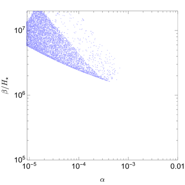
Figure 1: Scatter plot in the $(\alpha,\beta/H_{\star})$ plane for the minimal model.

3.4.2 Adding an auxiliary real scalar

Including an auxiliary real scalar field $\eta$ introduces a cubic term at zero temperature and, as in the case of electroweak baryogenesis, may increase the strength of the phase transition and GW production. In addition to the three parameters of the minimal model, we scan over $\widetilde{\mu}/v_{0}$, the parameter describing the zero-temperature cubic term.

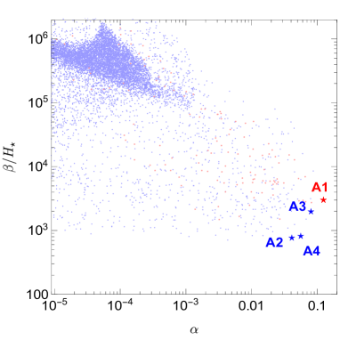
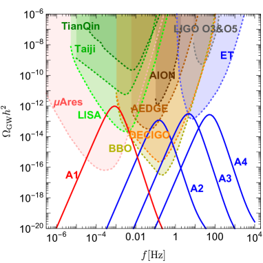
Figure 2: Quartic potential with zero temperature cubic term. Left panel: Scatter plot in the $(\alpha,\beta/H_{\star})$ plane. The blue (red) points correspond to the high scale (GeV seesaw scale) scenario. Right panel: GW spectra for the four benchmark points in Table 1 and marked with stars in the left panel.

The result of the scan is shown as blue points in the left panel of Fig. 2. The points fall in the region with $\alpha\lesssim 0.1$ and $\beta/H_{\star}\gtrsim 1000$. We select three benchmark points (A2, A3 and A4 marked with blue stars) whose parameters are in Table 1. The corresponding GW spectra are displayed in the right panel; the scale of the phase transition covers many orders of magnitude, from $\sim$100 GeV to $\sim$PeV. The sensitivity of LIGO Aasi:2013wya ; Abbott:2021xxi and the future experiments, $\mu$Ares Sesana:2019vho , TianQin Luo:2015ght , Taiji Guo:2018npi , LISA Auclair:2019wcv , BBO Yagi:2011wg , DECIGO Kawamura:2019jqt , AEDGE Bertoldi:2019tck , AION Badurina:2019hst , ET Hild:2010id , are also shown. Clearly, the scenario is testable at AEDGE, DECIGO, BBO and ET.

	Inputs				Predictions
	$m_{S}/{\rm GeV}$	$\tilde{\mu}/{\rm GeV}$	$M/{\rm GeV}$	$v_{0}/{\rm GeV}$	$T_{\star}/{\rm GeV}$	$\alpha$	$\beta/H_{\star}$	$\widetilde{a}$
A1	$0.06190$	$0.0005857$	$0.5361$	$3.5873$	$0.6504$	$0.1248$	$2966$	$0.05951$
A2	$156.2$	$13.15$	$465.6$	$1014$	$721$	$0.04139$	$754.8$	$0.3886$
A3	$1036$	$13.72$	$7977$	$44424$	$9180$	$0.08012$	$1975$	$0.06268$
A4	$43874$	$1856$	$181099$	$567378$	$247807$	$0.05611$	$809.7$	$0.1944$

Table 1: Values of the parameters corresponding to the four benchmark (starred) points in Fig. 2.

3.4.3 Nonthermal RH neutrinos

We now consider the case with a nonthermal RH neutrino abundance which introduces a logarithmic term in the effective potential. We set the zero-temperature cubic term $\widetilde{\mu}=0$ so that the potential depends on the nonthermal RH neutrino abundance $N_{N_{1}}$ in addition to the three parameters of the minimal model.

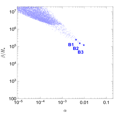
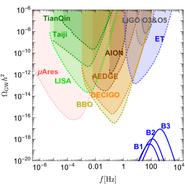
Figure 3: Potential with logarithmic field dependence and no cubic term at zero temperature. Left panel: Scatter plot in the $(\alpha,\beta/H_{\star})$ plane. Right panel: GW spectra for the three benchmark points in Table 2 and marked with stars in the left panel.

The result of the scan is shown in the left panel of Fig. 3. We select three benchmark points (B1, B2 and B3 marked with stars) and shown the corresponding GW spectra in the right panel; see Table 2 for the parameter values. Although the GW signals are enhanced compared to the minimal model, they are several orders of magnitude below the experimental sensitivity.

	Inputs				Predictions
	$m_{S}\over{\rm GeV}$	$N_{N_{1}}$	$M\over{\rm GeV}$	$v_{0}\over{\rm GeV}$	$T_{\star}\over{\rm GeV}$	$\alpha$	$\beta/H_{\star}$	$a_{0}$	$a_{1}$
B1	$1383$	$3.710$	$1523$	$1524$	$991.4$	$0.004190$	$247858$	$-0.04945$	$4.314$
B2	$3225$	$3.968$	$3763$	$3882$	$2331$	$0.006232$	$152233$	$2.898$	$8.775$
B3	$19003$	$7.108$	$17724$	$20947$	$11682$	$0.009441$	$121398$	$3.1422$	$9.1367$

Table 2: Values of the parameters corresponding to the three benchmark (starred) points in the left panel of Fig. 3 and with GW spectra shown in the right panel of the same figure.

Our results are consistent with the general analysis presented in Ref. Ellis:2020awk for potentials of the same form. However, in our case the range of $(\alpha,\beta/H_{\star})$ in the scatter plot is not spanned because the number of degrees of freedom in the dark sector is a small fraction of the SM value. Hence, the GW signal is always weaker than, for example, from electroweak baryogenesis. The situation is better in low scale scenarios, but there is a price to pay.

4 Low scale scenarios

So far we have assumed that the phase transition in the dark sector occurs at a temperature above the electroweak scale, when all SM degrees of freedom are in ultrarelativistic thermal equilibrium. We also assumed that all RH neutrinos acquire mass during the phase transition so that $T_{\star}$ approximately coincides with the seesaw scale, i.e., $T_{\star}\sim M$. In this section we relax either the first of these assumptions or both, thereby considering scenarios in which the phase transition occurs at temperatures below the electroweak scale, and the seesaw scale $M$ does not necessarily coincide with $T_{\star}$.

4.1 General considerations

There is an important consequence of this new setup. In high scale scenarios, the Yukawa couplings of the seesaw RH neutrinos couple the dark sector to the SM sector. During the phase transition the seesaw RH neutrinos acquire mass and then quickly decay. So the relic dark sector comprised of the two scalars $S$ and $J$ decouples after the phase transition and $T_{\rm dec}\simeq T_{\star}$. This is why we could take the dark sector and the SM thermal bath to have the same temperature during the phase transition, and calculate the effective thermal potential at the common temperature $T$. However, if the phase transition and seesaw scales are the same and lower than the electroweak scale, then from Eq. (6) with $K_{I}\lesssim 500$ (to avoid fine-tuning), the seesaw scale cannot be lower than $M\sim{\rm GeV}$ for $T^{\rm eq}_{I}\gtrsim 100\,{\rm GeV}$. Below this scale the seesaw RH neutrinos, and consequently the entire dark sector, will not thermalize and the maximum value of $\alpha$ sharply decreases, suppressing the GW signal.

4.2 GeV seesaw scale scenario

The possibility that the seesaw scale can be as low as $M\sim{\rm GeV}$ has been intensively investigated since it offers an avenue to test the seesaw mechanism directly at colliders and via meson decays, and also because such an extension of the SM does not destabilize the electroweak scale, thus complying with naturalness. Moreover, for RH neutrinos in the GeV mass range, the matter-antimatter asymmetry of the universe can be explained by leptogenesis from RH neutrino oscillations Akhmedov:1998qx .

We consider a scenario with $T_{\rm dec}=T_{\star}\sim M\sim{\rm GeV}$. Then, $g_{\rho}(T_{\star}\sim{\rm GeV})=61.75$ which increases the value of $\alpha$ (see Eq. 46) compared to the high scale scenarios. The red points and benchmark point A1 in the left panel of Fig. 2 correspond to this scenario. The parameter values for A1 and its GW spectrum are provided in Table 1 and the right panel of Fig. 2. Indeed, the GW signal has a higher peak than for the high scale benchmark points, and the peak frequency lies within LISA’s sensitivity range. It is noteworthy that LISA is more sensitive to low scale phase transitions with $\beta/H_{\star}\simeq 1000$, than electroweak scale phase transitions for which $\beta/H_{\star}\simeq 10$–100 is typically assumed.

4.3 Splitting the seesaw and the phase transition scales

As another class of low scale scenarios, we consider a phase transition scale much below a GeV. For the time being, the two heaviest RH neutrinos, which we refer to as seesaw RH neutrinos, are assumed to couple the two sectors at temperature $T\sim M\gtrsim 1\,{\rm GeV}$. (Later, we will relax this assumption and also consider other options.) Since $T_{\star}\ll M$, the two seesaw RH neutrinos do not acquire mass $\sim M$ during the $\sigma$-phase transition. Instead, they may gain their mass during an earlier phase transition at $T\sim M$, as for example, in the case with an additional real scalar $\eta$. While this will not play a role in our immediate considerations, it is interesting that a double peaked GW spectrum may result, with one peak at a high frequency and a second peak at a lower frequency. The $\sigma$-phase transition will then give a mass only to the lightest RH neutrino $N_{1}$, and, possibly, to additional lighter RH neutrinos. We continue to denote the mass scale of the two heavy seesaw RH neutrinos by $M$. We will denote the common mass of the light RH neutrinos generated during the $\sigma$-phase transition by $M^{\prime}$, and their number by $N^{\prime}(=N-2)$. If there are no additional light RH neutrinos beyond $N_{1}$, then $N^{\prime}=1$.

For now we also assume that the $N^{\prime}$ light RH neutrinos, and consequently the whole dark sector, does not recouple prior to the phase transition, and therefore $T_{\rm dec}\simeq M\gg T_{\star}$. Then, at the phase transition the dark sector has a temperature $T^{\prime}<T$. Our expressions for the thermal effective potential continue to hold with the replacement $T\rightarrow T^{\prime}$. One then needs to express $T^{\prime}$ as a function of $T$. This can be easily done by requiring entropy conservation between decoupling and the phase transition. Introducing the entropy number degrees of freedom $g_{s}(T)$, the total entropy density is

$$s(T)={2\pi^{2}\over 45}\,g_{s}(T)\,T^{3}\,.$$ (72)

Like the energy density, this can be split into a contribution from the SM sector and a contribution from the dark sector. Since the dark sector is at temperature $T^{\prime}$ when the SM sector is at temperature $T$, $s(T)=s_{\rm SM}(T)+s_{\rm dark}(T^{\prime}(T))$. Both contributions in turn can be expressed in terms of their respective entropy number of degrees of freedom via

$$s_{\rm SM}(T)={2\pi^{2}\over 45}\,g_{s}^{\rm SM}(T)\,T^{3}\,\;\;\;\;\;\mbox{\rm and}\;\;\;\;\;s_{\rm dark}(T^{\prime}(T))={2\pi^{2}\over 45}\,g_{\rm dark}(T)\,T^{3}\,r_{T}^{3}\,,$$ (73)

where $r_{T}\equiv T^{\prime}/T$ and $g_{\rm dark}(T)\equiv g_{\rm dark}(T^{\prime}(T))$. With this definition of $g_{\rm dark}(T)$, we can write $g_{s}(T)=g_{s}^{\rm SM}(T)+g_{\rm dark}(T)\,r_{T}^{3}$. We assume that when the two seesaw RH neutrinos decay, their entropy is redistributed in both sectors so that $r_{T}(T_{\rm dec})=1$. In the dark sector, before the phase transition, $g_{\rm dark}(T)$ receives a contribution from the scalars, $g_{\sigma+\eta}=3$, and a contribution from the $N^{\prime}$ light RH neutrinos, $g_{N^{\prime}}=7\,N^{\prime}/4$. After decoupling, $g_{\rm dark}$ can be assumed to be constant until the phase transition. Analogously to the standard calculation of the evolution of the ordinary neutrino temperature after decoupling, we find

$$r_{T}(T_{\rm dec},T_{\star})=\left[{g^{\rm SM}_{s}(T_{\star})\over g^{\rm SM}_{s}(T_{\rm dec})}\right]^{1/3}\,.$$ (74)

We further assume that after the phase transition, the massive scalar $S$ and the $N^{\prime}$ light RH neutrinos decay so that $g_{\rm dark}(T<T_{\star})=2$. In the next subsection we apply this general setup to a specific interesting scenario.

4.4 Phase transitions below an MeV, NANOGrav, and the Hubble tension

An interesting possibility is whether the class of low scale scenarios with $T_{\star}\ll M$ can address the recent NANOGrav results which show evidence for the existence of a stochastic GW background at $\sim 10^{-8}\,{\rm Hz}$ Arzoumanian:2020vkk . For $\beta/H_{\star}\gtrsim 1000$, Eq. (52) indicates $T_{\star}\lesssim 100\,{\rm keV}$. The crucial question is if the amplitude of the NANOGrav signal, $h^{2}\,\Omega_{\rm GW0}(f)\sim 10^{-10}$, is reproducible. We will find that reproducing the NANOGrav signal is challenging Arzoumanian:2021teu . However, the predicted GW signal can be well within the reach of future experiments such as SKA Janssen:2014dka and THEIA THEIA . Quite interestingly, such a phase transition scale is independently motivated by the Hubble tension, as we discuss below.

For $T_{\star}\lesssim 100\,{\rm keV}$, well below the electron mass, the standard result $g^{\rm SM}_{s}(T_{\star})=43/11$ holds and, since $g^{\rm SM}_{s}(T_{\rm dec}\gtrsim 100\,{\rm GeV})=106.75$, Eq. (74) gives $r_{T}(T_{\rm dec}\gtrsim 100\,{\rm GeV},T_{\star}\lesssim 100\,{\rm keV})\simeq 0.33$. To calculate $\alpha$ from Eq. (46), we also need

$$g_{\rho}^{\rm SM}(T_{\star})=2+{7\over 4}\times 3.044\times\left({4\over 11}\right)^{4\over 3}\simeq 3.36\,,$$ (75)

where $N_{\nu}^{\rm eff,SM}\simeq 3.044$ is the effective number of ultrarelativistic neutrino species in the SM Bennett:2020zkv ; Akita:2020szl . The left panel of Fig. 4 shows for $N^{\prime}=1$ that only $\alpha\lesssim 0.01$ and $\beta/H_{\star}\gtrsim 10^{4}$ are allowed. We select three benchmark points (C1, C2 and C3) that maximize the GW signal (shown in the right panel of Fig. 4; the parameter values are in Table 3). The signal peaks are many orders of magnitude below the NANOGrav result and even below the sensitivity of future experiments like SKA and THEIA.

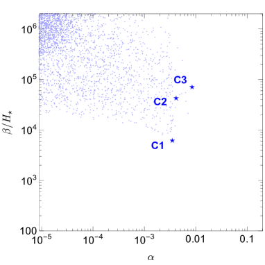
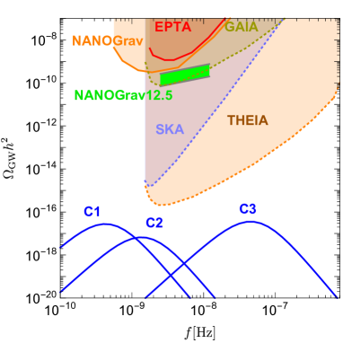
Figure 4: Low scale scenario for $T_{\rm dec}\gtrsim 100\,{\rm GeV}$ and $T_{\star}\lesssim 100\,{\rm keV}$. Left panel: Scatter plot in the $(\alpha,\beta/H_{\star})$ plane. Right panel: GW spectra for the three benchmark points in Table 3 and marked with stars in the left panel.

	Inputs				Predictions
	$m_{S}/{\rm keV}$	$\tilde{\mu}/{\rm keV}$	$M/{\rm keV}$	$v_{0}/{\rm keV}$	$T_{\star}/{\rm keV}$	$\alpha$	$\beta/H_{\star}$	$\widetilde{a}$
C1	$0.08266$	$0.00002456$	$0.04838$	$0.09244$	$0.3949$	$0.003506$	$6206$	$0.5358$
C2	$0.01065$	$0.000303$	$0.03155$	$0.02364$	$0.1833$	$0.004152$	$42997$	$0.7945$
C3	$0.5266$	$0.2216$	$0.8440$	$0.2836$	$3.831$	$0.008528$	$70771$	$0.9583$

Table 3: Values of the parameters corresponding to the three benchmark (starred) points in Fig. 4.

Consider the possibility that the NANOGrav signal can be reproduced if the seesaw scale is lowered to a GeV, which as we have seen, permits thermalization of the SM and dark sectors. We set $T_{\rm dec}\sim 1\,{\rm GeV}$ and obtain $r_{T}(T_{\rm dec}\sim 1\,{\rm GeV},T_{\star}\lesssim{\rm 100keV})\simeq 0.40$. This increases $\alpha$ with respect to the previous case (with $T_{\rm dec}\gtrsim 100\,{\rm GeV}$) by a factor $\sim(106.75/61.75)^{4/3}\sim(0.40/0.33)^{4}\simeq 2$. Since the peak of the GW spectrum $\sim\alpha^{5}$ (accounting for the fact that $\beta/H_{\star}\propto\alpha^{-2}$ Ellis:2020awk ) this increases the signal by a factor $\sim 38$, which is clearly insufficient to explain the NANOGrav signal and one can only marginally obtain testable signals at planned experiments.

Yet another possibility follows from the assumption that some additional interactions rethermalize the dark sector with photons. Then, $r_{T}=1$ which enhances the peak of the GW spectrum by a factor of $\sim 10^{9}$. Although this is sufficient to reproduce the NANOGrav signal, one must contend with cosmological constraints, as we discuss below.

We may also allow the number of light RH neutrinos $N^{\prime}$ to be larger than unity. This is expected to increase the GW signal since these neutrinos contribute to the thermal effective potential; see Eqs. (19) and (20) with $N$ replaced by $N^{\prime}$. From this point of view $N^{\prime}$ may be regarded as an effective number of light RH neutrinos that represent a higher complexity of the dark sector.

4.4.1 Cosmological constraints on dark radiation

Before proceeding, we pause to consider cosmological constraints on the extra radiation from the epochs of Big Bang Nucleosynthesis (BBN) and recombination. At temperatures $T\ll M$, the extra degrees of freedom are the $N^{\prime}$ light RH neutrinos and the scalars $\eta,S$ and $J$. The number of extra degrees of freedom at temperatures much below the muon mass is traditionally expressed in terms of the effective number of extra neutrino species $\Delta N_{\nu}^{\rm eff}(T)$ via

$$g_{\rho}(T)=g_{\rho}^{\rm SM}(T)+{7\over 4}\,\Delta N_{\nu}^{\rm eff}(T)\,[r_{T}^{\nu}(T)]^{4}\,,$$ (76)

where

$$r_{T}^{\nu}(T)=\left({2\over 11}\right)^{1\over 3}\,[g_{s}^{\gamma+e^{\pm}}(T)]^{1\over 3}\,,$$ (77)

with

$$g_{s}^{\gamma+e^{\pm}}(T)=2+{45\over\pi^{4}}\,\int_{0}^{\infty}\,dx\,{x^{2}\,\sqrt{x^{2}+z^{2}}+{1\over 3}\,{x^{2}\over\sqrt{x^{2}+z^{2}}}\over e^{\sqrt{x^{2}+z^{2}}}+1}\,.$$ (78)

Here, $z\equiv m_{\rm e}/T$. Primordial helium-4 abundance measurements combined with the baryon abundance extracted from Cosmic Microwave Background (CMB) anisotropies place a constraint on $\Delta N_{\nu}^{\rm eff}(t)$ at $t=t_{\rm f}\sim 1\,{\rm s}$, the time of freeze-out of the neutron-to-proton ratio Fields:2019pfx :

$$\Delta N_{\nu}^{\rm eff}(t_{\rm f})\simeq-0.1\pm 0.3\ \Rightarrow\ \Delta N_{\nu}^{\rm eff}(t_{\rm f})\lesssim 0.5\,\ \ (95\%\,{\rm C.L.})\,.$$ (79)

Measurements of the primordial deuterium abundance place a constraint on $\Delta N_{\nu}^{\rm eff}(t)$ at the time of nucleosynthesis, $t_{\rm nuc}\simeq 310\,{\rm s}$, corresponding to $T_{\rm nuc}\simeq 65\,{\rm keV}$ DiBari:2018vba :

$$\Delta N_{\nu}^{\rm eff}(t_{\rm nuc})=-0.2\pm 0.3\ \Rightarrow\ \Delta N_{\nu}^{\rm eff}(t_{\rm nuc})\lesssim 0.4\,\ \ (95\%\,{\rm C.L.})\,.$$ (80)

CMB temperature and polarization anisotropies constrain $\Delta N_{\nu}^{\rm eff}(t)$ at recombination, when $T\simeq T_{\rm rec}\simeq 0.3\,{\rm eV}$, and the Planck collaboration finds Aghanim:2018eyx

$$\Delta N_{\nu}^{\rm eff}(t_{\rm rec})=-0.06\pm 0.17\ \Rightarrow\ \Delta N_{\nu}^{\rm eff}(t_{\rm rec})\lesssim 0.3\,\ \ (95\%\,{\rm C.L.})\,.$$ (81)

We now calculate $\Delta N_{\nu}^{\rm eff}(t)$ for the Majoron model with the addition of a real scalar $\eta$. Assuming that the dark sector decouples at a temperature $T_{\rm dec}\gtrsim 1\,{\rm GeV}$ and does not recouple to the SM sector, the value of $\Delta N_{\nu}^{\rm eff}$ is constant throughout BBN until recombination. We evaluate $\Delta N_{\nu}^{\rm eff}$ below $T\sim m_{e}/2\simeq 250\,{\rm keV}$ so that $r_{T}^{\nu}(T)\simeq(4/11)^{1/3}$, and obtain

$$\Delta N_{\nu}^{\rm eff}(t_{\star})={4\over 7}\,\left({11\over 4}\right)^{4\over 3}\,r_{T}^{4}\,g_{\rm dark}(T)\,,$$ (82)

with $g_{\rm dark}(T)=3+{7\over 4}\,N^{\prime}$. In the canonical case with $T_{\rm dec}\gtrsim 100\,{\rm GeV}$ and $N^{\prime}=1$, we have $r_{T}=0.33$ and $\Delta N_{\nu}^{\rm eff}(t_{\star})\simeq 0.12$. In the low scale seesaw scenario with $T_{\rm dec}\simeq 1\,{\rm GeV}$ and $N^{\prime}=1$, we have $r_{T}=0.4$ and $\Delta N_{\nu}^{\rm eff}(t_{\star})\simeq 0.27$. These results are easily compatible with the BBN constraints. After the phase transition and prior to recombination, the lightest RH neutrinos and scalar $S$ acquire mass and behave as matter before decaying. Because these particles redshift like matter, the later they decay, the greater the contribution to $\Delta N_{\nu}^{\rm eff}$ at recombination. Thus, their lifetimes must be bounded from above.

If some new interactions fully rethermalize the dark sector prior to the phase transition, i.e., $r_{T}=1$, then for $N^{\prime}=1$, $\Delta N_{\nu}^{\rm eff}(T_{\star})\simeq 10$. This result could be put in agreement with BBN constraints if the late thermalization occurs just prior to the phase transition and $T_{\star}\lesssim 65\,{\rm keV}$, but it would be in obvious disagreement with the CMB anisotropies. There is, however, another interesting possibility to be considered.

4.4.2 GW signals and the Hubble tension

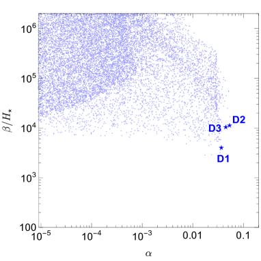
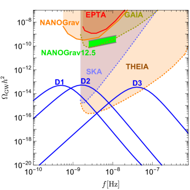
Figure 5: Rethermalization scenario with $r_{T}=0.6$ and $N^{\prime}=1$. Left panel: Scatter plot in the $(\alpha,\beta/H_{\star})$ plane. Right panel: GW spectra for the three benchmark points in Table 4 and marked with stars in the left panel.

The so-called Hubble tension Bernal:2016gxb between the CMB measurement of $H_{0}$ within $\Lambda$CDM and low-redshift astrophysical measurements suggest $\Delta N_{\nu}^{\rm eff}(t_{\rm rec})\simeq 0.6$. We calculate the maximum value of $r_{T}$ by very conservatively requiring $\Delta N_{\nu}^{\rm eff}(T_{\star})\lesssim 1.35$ to address the Hubble tension. From Eq. (82) with $N^{\prime}=1$, we find $r_{T}\simeq 0.6$. The result of our scan with $r_{T}=0.6$ is shown in the left panel of Fig. 5. Higher values of $\alpha$ and lower values of $\beta/H_{\star}$ can be obtained compared to the case with $r_{T}=0.33$ presented in Fig. 4. From the right panel we see that the GW spectra for three benchmark points can be detected at SKA and THEIA although their peaks are still three orders of magnitude below the NANOGrav signal.

	Inputs				Predictions
	$m_{S}/{\rm keV}$	$\tilde{\mu}/{\rm keV}$	$M/{\rm keV}$	$v_{0}/{\rm keV}$	$T_{\star}/{\rm keV}$	$\alpha$	$\beta/H_{\star}$	$\widetilde{a}$
D1	$0.083651$	$0.009534$	$0.3574$	$0.4082$	$0.8076$	$0.03641$	$4046$	$0.6795$
D2	$0.2650$	$0.9064$	$0.5571$	$0.2505$	$0.9902$	$0.05283$	$11407$	$0.9207$
D3	$5.4732$	$0.9724$	$14.19$	$8.341$	$26.13$	$0.04452$	$10472$	$0.8831$

Table 4: Values of the parameters corresponding to the three benchmark (starred) points in Fig. 5.

This scenario, however, is not only too generic, since we have not specified the interactions that cause rethermalization, but also unrealistic, since we have assumed that the dark sector essentially equilibrates with photons. Also, CMB data now clearly show that a mere injection of extra radiation at the level of $\Delta N_{\nu}^{\rm eff}\simeq 0.6$, though able to yield a higher value of $H_{0}$ from CMB anisotropies in agreement with the astrophysical measurements, results in a worse global fit of the data. This is because the extra radiation also produces a shift in the acoustic peaks which is not tolerated by current CMB data Knox:2019rjx . To ameliorate the Hubble tension within an extension of $\Lambda$CDM and provide a better global fit to the data requires a reduction of the sound horizon at recombination without an alteration of other CMB observables that are well fitted.

It is quite interesting that the requirements of specifying the interaction within a realistic model and producing a better cosmological global fit can be neatly satisfied within our Majoron model with split seesaw and phase transition scales. We introduce an interaction of the Majoron $J$ with the ordinary neutrino cosmic background of the type,

$$-{\cal L}_{\rm\nu-{\rm dark}}={i\over 2}\,\sum_{i=2,3}\lambda_{i}\,\overline{\nu_{i}}\,\gamma^{5}\,\nu_{i}\,\eta+{i\over 2}\,\lambda_{1}\overline{\nu_{1}}\,\gamma^{5}\,\nu_{1}\,J+{\rm h.c.}\,,$$ (83)

where $\nu_{2,3}$ are the two heavier ordinary neutrinos with masses generated by the seesaw and $\nu_{1}$ is the lightest ordinary neutrino that couples to the Majoron. Indeed, the interaction between dark radiation and neutrinos is just the ingredient needed to reduce the sound horizon and obtain a larger value of $H_{0}$ from the CMB anisotropies. The impact of this kind of interaction on the CMB was first studied in Ref. Chacko:2003dt and it has been recently considered in Refs. Escudero:2019gvw ; Escudero:2021rfi in the context of the Hubble tension. We have introduced a flavor dependence since in our case the seesaw scale and the phase transition scale are different. However, from the point of view of the CMB anisotropies the flavor dependence has no effect. (This kind of model falls into a more general class of models recently discussed in Ref. Blinov:2020hmc , also in relation to the Hubble tension. A recent example of a specific model within this class, though not a Majoron model, has been recently discussed in Ref. Choi:2020pyy .) The interactions in Eq. (83) partly rethermalizes the dark sector with the ordinary neutrinos such that

$$r_{T}=\left({4\over 11}\right)^{1\over 3}\,\left({3.044\over 3.044+N^{\prime}+12/7}\right)^{1\over 4}\,.$$ (84)

For $N^{\prime}=1$, we again find $r_{T}\simeq 0.6$. Also,

$$\Delta N_{\nu}^{\rm eff}(t_{\rm rec})\simeq 3.044\,\left({3.044+N^{\prime}+12/7\over 3.044+N^{\prime}+12/7-N_{\rm h}}\right)^{1\over 3}-3.044\simeq 0.5\,,$$ (85)

where $N_{\rm h}$ (equal to 2 in our case) is the number of massive states that decay and produce the excess radiation. The value, $\Delta N_{\nu}^{\rm eff}\simeq 0.5$, nicely coincides with the best fit value found in Refs. Escudero:2019gvw ; Blinov:2020hmc with $\Delta\chi_{\rm min}^{2}=-12.2$ compared to the $\Lambda$CDM model; the fit includes the astrophysical determination of $H_{0}$. The best fit values for the coupling constant and Majoron mass are $\lambda_{i}\sim 10^{-12}$ and $m_{J}\sim{\cal O}(0.1\,{\rm eV})$. It is quite intriguing that such values for the Majoron mass can be accommodated in phase transitions with $T_{\star}\sim{\rm keV}$. These values give rise to GW signals in the $10^{-8}\,{\rm Hz}$ range tested by NANOGrav, SKA and THEIA.

The interactions in Eq. (83) now provide a realistic way to achieve rethermalization of the dark sector and justifies $r_{T}\simeq 0.6$ which links possible GW signals at $\sim 10^{-8}\,{\rm Hz}$ to the Hubble tension. Effectively, the interaction causes ordinary neutrinos to be treated as part of the dark sector rather than the SM sector. Compared to the case in which the dark sector thermalizes with photons, now the thermal coupling between the dark sector and ordinary neutrinos also affects the value of $g_{\rho}^{\rm SM}(T_{\star})$, and therefore the value of $\alpha$. This is because the neutrino-to-photon temperature ratio decreases from the standard value $r^{\nu}_{T}=T_{\nu}/T=(4/11)^{1\over 3}$ to $r_{T}$. The total number of SM ultrarelativistic degrees of freedom at the phase transition decreases from the standard value $g_{\rho}^{\rm SM}\simeq 3.36$ to

$$g_{\rho}^{\rm SM^{\prime}}(T_{\star}\lesssim 100\,{\rm keV})=2+3.044\,{7\over 4}\,r_{T}^{4}\,.$$ (86)

For $r_{T}=0.6$, $g_{\rho}^{\rm SM^{\prime}}(T_{\star}\lesssim 100\,{\rm keV})\simeq 2.69$. On the other hand, the contribution from the dark sector is

$$g_{\rho}^{\rm dark}(T_{\star}\lesssim 100\,{\rm keV})={7\over 4}\,\left({4\over 11}\right)^{4\over 3}\,\Delta N_{\nu}^{\rm eff}(t_{\star})\,\,,$$ (87)

where $\Delta N_{\nu}^{\rm eff}(t_{\star})$ is given by Eq. (82).

We have so far considered the case $N^{\prime}=1$ corresponding to the usually considered total number of RH neutrinos $N=3$. However, we can also study how the GW signal changes with increasing $N^{\prime}$. In this context, $N^{\prime}$ should be regarded as an effective number of light RH neutrinos parameterizing an extension of the dark sector that contributes to the effective thermal potential. The result, not surprisingly, is that the GW signal is enhanced by increasing $N^{\prime}$, but the enhancement saturates for $N^{\prime}\sim 10$ as can be seen from the right panel of Fig. 6. We have selected five benchmark points with $N^{\prime}=1,3,5,7,10$, and whose GW spectra peak in the range of frequencies tested by NANOGrav, SKA and THEIA. The reason for the saturation is that for a given choice of all the other parameters, there is an upper bound on the value of $N^{\prime}$ imposed by the stability of the potential, since the quartic coupling $\lambda_{T}$ in Eq. (20) becomes negative for too large $N$. Note that for $N^{\prime}=10$, Eq. (82) gives $\Delta N_{\nu}^{\rm eff}(t_{\rm nuc})=0.535$, in conflict with the BBN constraint in Eq. (80). However, this can be circumvented by relaxing our assumption that the dark sector undergoes an early thermalization at temperatures above $\sim 100\,{\rm GeV}$ and then rethermalizes at low temperatures. Instead of rethermalization, the dark sector could thermalize for the first time at low temperatures prior to the phase transition.

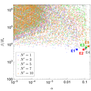
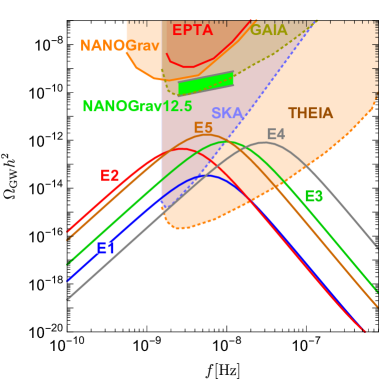
Figure 6: Rethermalization scenario addressing the Hubble tension. Left panel: Scatter plot in the $(\alpha,\beta/H_{\star})$ plane. Right panel: GW spectra for the five benchmark points E1–E5 in Table 5 corresponding to $N^{\prime}=1,3,5,7,10$, respectively, and marked with stars in the left panel.

	Inputs				Predictions
	$m_{S}/{\rm keV}$	$\tilde{\mu}/{\rm keV}$	$M/{\rm keV}$	$v_{0}/{\rm keV}$	$T_{\star}/{\rm keV}$	$\alpha$	$\beta/H_{\star}$	$\widetilde{a}$
E1	$0.6847$	$0.04274$	$2.795$	$3.507$	$7.036$	$0.03505$	$5286$	$0.7226$
E2	$0.3065$	$0.008314$	$1.401$	$3.253$	$3.711$	$0.08406$	$5229$	$0.4638$
E3	$0.7224$	$0.01154$	$3.808$	$12.34$	$10.33$	$0.1186$	$6993$	$0.7279$
E4	$2.620$	$0.05962$	$10.27$	$35.12$	$36.26$	$0.1086$	$5919$	$0.3974$
E5	$0.2771$	$0.003530$	$1.402$	$7.101$	$5.207$	$0.1609$	$8176$	$0.2127$

Table 5: Values of the parameters corresponding to the five benchmark (starred) points in Fig. 6.

These results are quite intriguing, since they show how a solution to the Hubble tension motivates a GW signal from a strong first-order phase transition in Majoron models within NANOGrav’s range of frequencies. We also see that even increasing $N^{\prime}$ yields GW spectra with peaks two orders of magnitude below the NANOGrav signal. We do not expect that a proper accounting of theoretical uncertainties or a calculation of the signal-to-noise ratio can overcome the two orders of magnitude needed to explain the NANOGrav signal.

5 Final remarks and conclusion

We discussed how a stochastic GW background may be generated in the early universe from first-order phase transitions in Majoron models. We considered high scale scenarios, in which the phase transition occurs above the electroweak scale, and low scale scenarios in which the phase transition occurs below the electroweak scale.

We highlight some aspects of our study.

• We have not introduced couplings of the complex scalar $\sigma$ to the Higgs boson. So the Higgs sector is not modified, for example by a Higgs portal operator $\propto H^{\dagger}H\,|\sigma|^{2}$. In the high scale scenarios, with $v_{0}\gg v_{\rm ew}$, it can be assumed that the coupling is small to not destabilize the electroweak scale and introduce a naturalness problem. Below the electroweak scale, this term would simply contribute to the quadratic term and be incorporated into $\mu^{2}$. We have also not explicitly considered nonrenormalizable higher dimensional operators so that our model is ultraviolet-complete.

• In high scale scenarios the GW signal can be detected at currently planned interferometers.

• The stability of the effective potential limits the size of the GW signal at low frequencies in the low scale scenarios to two or more orders of magnitude below the NANOGrav signal. If the NANOGrav signal is confirmed then a more drastic departure from the models presented here needs to be considered.

• For phase transitions in the dark sector, typically $\beta/H_{\star}\gtrsim 1000$ rather than $\beta/H_{\star}\gtrsim 10$–$100$, as usually assumed in the case of electroweak phase transitions. This shifts all signals to higher frequencies, which makes it desirable that experiments be planned with greater sensitivity in the range of frequencies relevant to ET. We find that LISA will test phase transitions at the GeV scale that may have connections with Majoron models, and with RH neutrino searches at FASER Ariga:2019ufm .

• In low scale scenarios we considered the possibility that the phase transition occurs even below the decoupling scale of ordinary neutrinos. In this case, a GW signal is generated in the range of frequencies currently probed by NANOGrav and may be observable at SKA and THEIA.

• The Hubble tension can be addressed in models in which the dark sector interacts with the ordinary neutrinos. This offers an intriguing connection between two apparently independent phenomenologies and makes it possible to test late thermalization scenarios and departures from $\Lambda$CDM with GW experiments.

Finally, we stress the inverse problem, i.e., the possibility of extracting the physical parameters that describe the phase transition from an observed GW signal. The peak frequency, amplitude and shape of the spectrum can help reconstruct the four thermodynamic parameters, $\alpha,T_{\star},\beta/H_{\star},v_{\rm w}$, that describe the phase transition despite the presence of degeneracies. Recently, it has been emphasized that a more realistic description of the sound wave contribution entails a double broken power law parameterized by four spectral parameters rather than just two for a single power law as in Eq. (50) Gowling:2021gcy . It should be said however that the situation for values of $\beta/H_{\star}\gtrsim 1000$, as in the case of a dark sector phase transition, is much more challenging than in the case of a phase transition in the visible sector such as the electroweak phase transition. For this reason it is important to have a specific model in which the GW signal may be linked to other phenomenological observables. Our study meets this requirement since there is a strong complementarity with other phenomenology, such as meson decays experiments for GeV scale scenarios, and cosmological tensions (i.e., departures from $\Lambda$CDM) in the case of very low energy scale scenarios. We have also seen how in the latter case a very interesting signature is the possibility of observing a double peak GW signal, one at high frequencies from seesaw RH neutrinos and one at low frequencies from light RH neutrinos.

Appendix A Appendix

In this Appendix we briefly discuss how to calculate $T_{\star}$ and derive Eq. (43). We also present analytical fits of the Euclidean action for a general effective potential. All results contained in this Appendix are applicable in general, and beyond Majoron models.

A.1 Calculation of $T_{\star}$

We defined the time of the phase transition by $I(t_{\star})=1$; see Eq. (42). A brute force method of calculating $T_{\star}$ is to plug an expression for the Euclidean action $S_{E}$ as a function of temperature into the equation, $I(t(T_{\star}))=1$, and solve it numerically. However, Eq. (42) can be simplified because in the detonation regime the duration of the phase transition is much shorter than the age of the universe. This is confirmed by the fact we always find $\beta/H_{\star}\gg 1$. We can then neglect the expansion during the phase transition and write,

$$I(t)\simeq{4\pi\over 3}\,v_{\rm w}^{3}\int_{t_{\rm c}}^{t}\,dt^{\prime}\,\Gamma(t^{\prime})\,(t-t^{\prime})^{3}\,.$$ (A.1)

Since we know the nucleation rate as a function of temperature,

$$\Gamma(T)\simeq T^{4}\,\left[{S_{E}(T)\over 2\pi}\right]^{3/2}\,e^{-S_{E}(T)}\,,$$ (A.2)

it is convenient to switch variables from time to temperature using $dt^{\prime}=-dT^{\prime}/[H(T^{\prime})\,T^{\prime}]\,$ and the usual relation in the radiation-dominated regime,

$$t={1\over 2}\,\sqrt{90\over 8\pi^{3}\,g_{\rho}(T)}\,{M_{\rm P}\over T^{2}}\,.$$ (A.3)

In terms of the dimensionless quantity $x\equiv T/v_{0}$, the condition $I(T_{\star})=1$ is equivalent to

$$h(x_{\star})=C(v_{0})\,,$$ (A.4)

where

$$h(x)\equiv\int_{x_{\star}}^{x_{\rm c}}\,dx^{\prime}\,x^{\prime}\,\left[{S_{E}(x^{\prime})\over 2\,\pi}\right]^{3\over 2}\,e^{-S_{E}(x^{\prime})}\,\left({1\over x^{2}}-{1\over x^{{}^{\prime}2}}\right)^{3}\,$$ (A.5)

and

$$C(v_{0})\equiv{H^{4}(v_{0})\over v_{0}^{4}}\,{6\over\pi\,v_{\rm w}^{3}}\,.$$ (A.6)

Although laborious, solving Eq. (A.4) for $T_{\star}$ is simpler than solving the original equation.

However, further simplification is possible by noting that Eq. (45) implies a linear expansion of the Euclidean action around $t_{\star}$ so that the nucleation rate in Eq. (A.1) can be written as $\Gamma(t)=\Gamma_{\star}\,e^{\beta(t-t_{\star})}$, where $\Gamma_{\star}\equiv\Gamma(t_{\star})$. Since the integral is dominated by $t\simeq t_{\star}$ Turner:1992tz ,

$$I(t)\simeq 8\,\pi\,v_{\rm w}^{3}\,{\Gamma_{\star}\over\beta^{4}}\,e^{\beta(t-t_{\star})}\,.$$ (A.7)

Using this expression in $I(t_{\star})=1$, gives Eq. (43). Clearly, Eq. (43) is much easier to solve if the Euclidean action is provided as a function of temperature. We verified that solving Eq. (43) gives results for $\alpha$ and $\beta/H_{\star}$ in full agreement with those obtained by solving Eq. (A.4).

An even simpler and numerically efficient procedure employs the facts that $T_{H}$ and $T_{\star}$ are very close to each other with $T_{H}>T_{\star}$, and that the derivative of the Euclidean action is approximately constant in the interval $[T_{\star},T_{H}]$. Then,

$$S_{E}(T_{\star})\simeq S_{E}(T_{H})-S^{\prime}_{E}(T_{H})\,(T_{H}-T_{\star})\,,$$ (A.8)

where $S_{E}(T_{H})$ is given by Eq. (44).

A.2 Analytical expression for the Euclidean action in the general case

We provide expressions for the function $f(a_{0},a_{1})$ in Eq. (70) for the Euclidean action obtained from the effective potential of Eq. (67).

The two vacua at $\langle\bar{\sigma}_{1}\rangle=0$ and $\langle\bar{\sigma}_{1}\rangle=(\sqrt{4a_{1}+1}-1)/a_{1}$ become degenerate at the critical temperature when the coefficients $a_{0}$ and $a_{1}$ satisfy the condition $a_{0}=a_{0}^{m}(a_{1})$, where

$$a_{0}^{m}(a_{1})\equiv a_{1}\left[\frac{2}{\sqrt{4a_{1}+1}-1}-1+2\log\left(\frac{\sqrt{4a_{1}+1}+1}{4}\right)\right]\,.$$ (A.9)

For a given $a_{1}$, the potential has a global minimum away from 0 only if $a_{0}<a_{0}^{m}(a_{1})$. In particular for $a_{1}=0$, $a_{0}<a_{0}^{m}(0)=1$, and for $a_{1}=2$, $a_{0}<a_{0}^{m}(0)=0$. In the presence of the logarithmic term, a positive $a_{1}$ guarantees the stability of the vacuum, irrespective of the sign of $a_{0}$. While $a_{0}<a_{0}^{m}(a_{1})$ with $0<a_{1}<+\infty$ is an ideal condition to trigger the first-order phase transition, we require $a_{0}<a_{0}^{m}(a_{1})-0.05$ to keep the numerical scan far away from the singularity at $a_{0}=a_{0}^{m}(a_{1})$.

Since a semi-analytical formula valid for the entire parameter space is challenging, we obtain two numerical fits for the 3-dimensional Euclidean action in two separate regions:

$$A = \{(a_{0},a_{1})|10^{-3}\leqslant a_{1}\leqslant 0.2,~{}10^{-4}\leqslant a_{0}<a_{0}^{m}(a_{1})-0.05\}\,,$$

$$B = \{(a_{0},a_{1})|0.2\leqslant a_{1}\leqslant 10,~{}-2\leqslant a_{0}<a_{0}^{m}(a_{1})-0.05\}\,.$$ (A.10)

For $(a_{0},a_{1})\in A$, we first fix the value of $a_{1}$. Then $a_{0}^{m}(a_{1})$, the maximum value of $a_{0}$, is also fixed. We scan $a_{0}$ in the interval $(0,a_{0}^{m}(a_{1})-0.05)$ and obtain a fit for $f(a_{0},a_{1})$. In region A, we fit a function of the form,

$$f(a_{0},a_{1}) = f_{0}(a_{1})+f_{1}(a_{1})a_{0}+\frac{f_{2}(a_{1})a_{0}}{\alpha^{m}_{0}-a_{0}}+\frac{f_{3}(a_{1})a_{0}}{(\alpha^{m}_{0}-a_{0})^{2}}\,.$$ (A.11)

Varying $a_{1}$ in the interval $[10^{-3},0.2]$, we obtain the following numerical fits for the $f_{i}$’s:

$$f_{0}(a_{1}) = \frac{5.31}{\left|a_{1}-2\right|^{1.18}}+\frac{17.17}{(a_{1}-2)^{2}}+\frac{48.78}{(a_{1}-2)^{3}}+\frac{70.59}{(a_{1}-2)^{4}}\,,$$

$$f_{1}(a_{1}) = \widetilde{f}_{0}(a_{1})e^{-1.91a_{1}}\left(\frac{-0.52}{a_{1}-2}-\frac{1.47a_{1}}{(a_{1}-2)^{2}}\right)\,,$$

$$f_{2}(a_{1}) = \widetilde{f}_{0}(a_{1})\frac{0.51a_{1}^{3/2}+1.14a_{1}-0.30\sqrt{a_{1}}+0.64}{a_{1}^{3/2}+1}\,,$$

$$f_{3}(a_{1}) = 0.04a_{1}\left|a_{1}-2\right|^{0.012}+\frac{5.37a_{1}}{(a_{1}-2)^{2}}+\frac{0.05a_{1}}{(a_{1}-2)^{3}}+\frac{0.02a_{1}}{(a_{1}-2)^{4}}+0.30\,.$$ (A.12)

In region B we express $f(a_{0},a_{1})$ in the form,

$$f(a_{0},a_{1}) = \frac{g_{1}(a_{1})}{(a_{0}^{m}(a_{1})-a_{0})^{2}}+\frac{g_{2}(a_{1})}{a_{0}^{m}(a_{1})-a_{0}}+\frac{g_{3}(a_{1})}{(a_{0}^{m}(a_{1})-a_{0})^{1/2}}+\frac{g_{4}(a_{1})}{(a_{0}^{m}(a_{1})-a_{0})^{1/4}}$$ (A.13)

$$+g_{5}(a_{1})\log(a_{0}^{m}(a_{1})-a_{0})\,,$$

and obtain the following numerical fits for the $g_{i}$’s:

$$g_{1}(a_{1}) = 0.45a_{1}+0.69\,,$$

$$g_{2}(a_{1}) = -0.40\cos\left(41.16-\frac{177.2}{\sqrt[4]{a^{\prime}_{1}}}+\frac{229.2}{\sqrt{a^{\prime}_{1}}}-\frac{120.6}{a^{\prime}_{1}}\right)+2.76\,,$$

$$g_{3}(a_{1}) = -3.59\cos\left(32.92-\frac{161.6}{\sqrt[4]{a^{\prime}_{1}}}+\frac{212.8}{\sqrt{a^{\prime}_{1}}}-\frac{112.0}{a^{\prime}_{1}}\right)+0.43\,,$$

$$\widetilde{g}_{4}(a_{1}) = 3.46\cos\left(26.40-\frac{161.3}{\sqrt[4]{a^{\prime}_{1}}}+\frac{211.9}{\sqrt{a^{\prime}_{1}}}-\frac{110.4}{a^{\prime}_{1}}\right)+0.71\,,$$

$$g_{5}(a_{1}) = -0.58\cos\left(29.6-\frac{146.5}{\sqrt[4]{a^{\prime}_{1}}}+\frac{193.6}{\sqrt{a^{\prime}_{1}}}-\frac{102.8}{a^{\prime}_{1}}\right)-0.04\,,$$ (A.14)

where $a^{\prime}_{1}=a_{1}+2$.

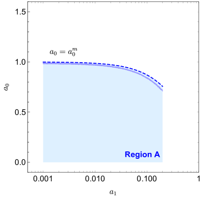
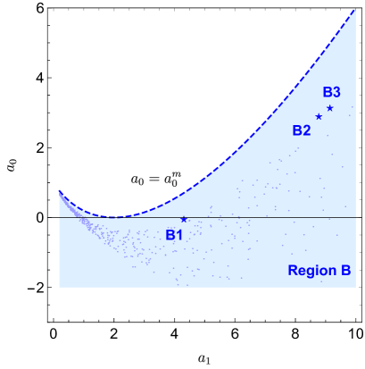
Figure 7: Scatter plots in the $(a_{0},a_{1})$ plane in the high-scale scenario with logarithmic field dependence and no cubic term at zero temperature. The benchmark points in Table 2 are marked with stars.

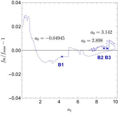
Figure 8: Errors in the fit function for region B. Starred points correspond to values of $a_{0}$ for the benchmark points in Table 2.

Values of $a_{0}$ and $a_{1}$ in region $A$ (left panel) and $B$ (right panel) are shown in Fig. 7. We verified that the analytical fits for $f(a_{0},a_{1})$ in regions A and B agree with the numerical results within $5\%$. Figure 8 shows the errors for values of $a_{0}$ that correspond to benchmark points B1, B2 and B3. We confirmed that in the limit $a_{1}\rightarrow 0$, we recover Eq. (64) with $a_{0}=\widetilde{a}$.

References

- (1) E. Witten, Cosmic Separation of Phases, Phys. Rev. D 30 (1984), 272-285.
- (2) C. J. Hogan, Gravitational radiation from cosmological phase transitions, Mon. Not. Roy. Astron. Soc. 218 (1986), 629-636.
- (3) M. S. Turner and F. Wilczek, Relic gravitational waves and extended inflation, Phys. Rev. Lett. 65 (1990), 3080-3083.
- (4) M. Kamionkowski, A. Kosowsky and M. S. Turner, Gravitational radiation from first-order phase transitions, Phys. Rev. D 49 (1994), 2837-2851 [arXiv:astro-ph/9310044 [astro-ph]].
- (5) R. Apreda, M. Maggiore, A. Nicolis and A. Riotto, Gravitational waves from electroweak phase transitions, Nucl. Phys. B 631 (2002), 342-368 [arXiv:gr-qc/0107033 [gr-qc]].
- (6) Y. Bai, A. J. Long and S. Lu, Dark Quark Nuggets, Phys. Rev. D 99 (2019) no.5, 055047 [arXiv:1810.04360 [hep-ph]].
- (7) F. P. Huang and C. S. Li, Probing the baryogenesis and dark matter relaxed in phase transition by gravitational waves and colliders, Phys. Rev. D 96 (2017) no.9, 095028 [arXiv:1709.09691 [hep-ph]].
- (8) E. Hall, T. Konstandin, R. McGehee and H. Murayama, Asymmetric Matters from a Dark First-Order Phase Transition, [arXiv:1911.12342 [hep-ph]].
- (9) P. Di Bari, D. Marfatia and Y. L. Zhou, Gravitational waves from neutrino mass and dark matter genesis, Phys. Rev. D 102 (2020) no.9, 095017 [arXiv:2001.07637 [hep-ph]].
- (10) Y. Chikashige, R. N. Mohapatra and R. D. Peccei, Are There Real Goldstone Bosons Associated with Broken Lepton Number?, Phys. Lett. B 98 (1981), 265-268.
- (11) Z. Arzoumanian et al. [NANOGrav], The NANOGrav 12.5 yr Data Set: Search for an Isotropic Stochastic Gravitational-wave Background, Astrophys. J. Lett. 905 (2020) no.2, L34 [arXiv:2009.04496 [astro-ph.HE]].
- (12) Y. Nakai, M. Suzuki, F. Takahashi and M. Yamada, Gravitational Waves and Dark Radiation from Dark Phase Transition: Connecting NANOGrav Pulsar Timing Data and Hubble Tension, Phys. Lett. B 816, 136238 (2021) [arXiv:2009.09754 [astro-ph.CO]].
- (13) L. Bian, R. G. Cai, J. Liu, X. Y. Yang and R. Zhou, Evidence for different gravitational-wave sources in the NANOGrav dataset, Phys. Rev. D 103 (2021) no.8, L081301 [arXiv:2009.13893 [astro-ph.CO]].
- (14) A. Addazi, Y. F. Cai, Q. Gan, A. Marciano and K. Zeng, NANOGrav results and Dark first-order Phase Transitions, [arXiv:2009.10327 [hep-ph]].
- (15) M. Breitbach, J. Kopp, E. Madge, T. Opferkuch and P. Schwaller, Dark, Cold, and Noisy: Constraining Secluded Hidden Sectors with Gravitational Waves, JCAP 07, 007 (2019) [arXiv:1811.11175 [hep-ph]].
- (16) M. Fairbairn, E. Hardy and A. Wickens, Hearing without seeing: gravitational waves from hot and cold hidden sectors, JHEP 07 (2019), 044 [arXiv:1901.11038 [hep-ph]].
- (17) B. Garbrecht, F. Glowna and P. Schwaller, Scattering Rates For Leptogenesis: Damping of Lepton Flavour Coherence and Production of Singlet Neutrinos, Nucl. Phys. B 877 (2013), 1-35 [arXiv:1303.5498 [hep-ph]].
- (18) P. Di Bari, K. Farrag, R. Samanta and Y. L. Zhou, Density matrix calculation of the dark matter abundance in the Higgs induced right-handed neutrino mixing model, JCAP 10 (2020), 029 [arXiv:1908.00521 [hep-ph]].
- (19) D. A. Kirzhnits and A. D. Linde, Macroscopic Consequences of the Weinberg Model, Phys. Lett. B 42 (1972), 471-474.
- (20) L. Dolan and R. Jackiw, Symmetry Behavior at Finite Temperature, Phys. Rev. D 9, 3320-3341 (1974).
- (21) G. W. Anderson and L. J. Hall, The Electroweak phase transition and baryogenesis, Phys. Rev. D 45 (1992), 2685-2698.
- (22) M. Dine, R. G. Leigh, P. Y. Huet, A. D. Linde and D. A. Linde, Towards the theory of the electroweak phase transition, Phys. Rev. D 46 (1992), 550-571 [arXiv:hep-ph/9203203 [hep-ph]].
- (23) M. Quiros, Finite temperature field theory and phase transitions, [arXiv:hep-ph/9901312 [hep-ph]].
- (24) C. Delaunay, C. Grojean and J. D. Wells, Dynamics of Non-renormalizable Electroweak Symmetry Breaking, JHEP 04, 029 (2008) [arXiv:0711.2511 [hep-ph]].
- (25) R. R. Parwani, Resummation in a hot scalar field theory, Phys. Rev. D 45 (1992), 4695 [erratum: Phys. Rev. D 48 (1993), 5965] [arXiv:hep-ph/9204216 [hep-ph]].
- (26) For a detailed discussion see: D. Curtin, P. Meade and H. Ramani, Thermal Resummation and Phase Transitions, Eur. Phys. J. C 78 (2018) no.9, 787 [arXiv:1612.00466 [hep-ph]].
- (27) For a recent critical study on theoretical uncertainties in daisy-resummed approach see: D. Croon, O. Gould, P. Schicho, T. V. I. Tenkanen and G. White, Theoretical uncertainties for cosmological first-order phase transitions, JHEP 04 (2021), 055 [arXiv:2009.10080 [hep-ph]].
- (28) A. Vilenkin, Cosmic Strings and Domain Walls, Phys. Rept. 121, 263-315 (1985).
- (29) T. W. B. Kibble, Topology of Cosmic Domains and Strings, J. Phys. A 9, 1387-1398 (1976).
- (30) Y. B. Zeldovich, I. Y. Kobzarev and L. B. Okun, Cosmological Consequences of the Spontaneous Breakdown of Discrete Symmetry, Zh. Eksp. Teor. Fiz. 67, 3-11 (1974) SLAC-TRANS-0165.
- (31) J. Choi and R. R. Volkas, Real Higgs singlet and the electroweak phase transition in the Standard Model, Phys. Lett. B 317 (1993), 385-391 [arXiv:hep-ph/9308234 [hep-ph]].
- (32) J. Kehayias and S. Profumo, Semi-Analytic Calculation of the Gravitational Wave Signal From the Electroweak Phase Transition for General Quartic Scalar Effective Potentials, JCAP 03, 003 (2010) [arXiv:0911.0687 [hep-ph]].
- (33) S. R. Coleman, The Fate of the False Vacuum. 1. Semiclassical Theory, Phys. Rev. D 15 (1977), 2929-2936 [erratum: Phys. Rev. D 16 (1977), 1248].
- (34) A. D. Linde, Decay of the False Vacuum at Finite Temperature, Nucl. Phys. B 216 (1983), 421 [erratum: Nucl. Phys. B 223 (1983), 544].
- (35) A. H. Guth and S. H. H. Tye, Phase Transitions and Magnetic Monopole Production in the Very Early Universe, Phys. Rev. Lett. 44 (1980), 631 [erratum: Phys. Rev. Lett. 44 (1980), 963].
- (36) A. H. Guth and E. J. Weinberg, Cosmological Consequences of a first-order Phase Transition in the SU(5) Grand Unified Model, Phys. Rev. D 23 (1981), 876
- (37) A. Megevand and S. Ramirez, Bubble nucleation and growth in very strong cosmological phase transitions, Nucl. Phys. B 919 (2017), 74-109 [arXiv:1611.05853 [astro-ph.CO]].
- (38) J. Ellis, M. Lewicki and J. M. No, Gravitational waves from first-order cosmological phase transitions: lifetime of the sound wave source, JCAP 07 (2020), 050 [arXiv:2003.07360 [hep-ph]].
- (39) C. Caprini, M. Hindmarsh, S. Huber, T. Konstandin, J. Kozaczuk, G. Nardini, J. M. No, A. Petiteau, P. Schwaller and G. Servant, et al. Science with the space-based interferometer eLISA. II: Gravitational waves from cosmological phase transitions, JCAP 04 (2016), 001 [arXiv:1512.06239 [astro-ph.CO]].
- (40) C. Caprini, M. Chala, G. C. Dorsch, M. Hindmarsh, S. J. Huber, T. Konstandin, J. Kozaczuk, G. Nardini, J. M. No and K. Rummukainen, et al. Detecting gravitational waves from cosmological phase transitions with LISA: an update, JCAP 03 (2020), 024 [arXiv:1910.13125 [astro-ph.CO]].
- (41) P. J. Steinhardt, Relativistic Detonation Waves and Bubble Growth in False Vacuum Decay, Phys. Rev. D 25, 2074 (1982).
- (42) J. R. Espinosa, T. Konstandin, J. M. No and G. Servant, Energy Budget of Cosmological First-order Phase Transitions, JCAP 06, 028 (2010) [arXiv:1004.4187 [hep-ph]].
- (43) J. Ellis, M. Lewicki and J. M. No, On the Maximal Strength of a First-Order Electroweak Phase Transition and its Gravitational Wave Signal, JCAP 04 (2019), 003 [arXiv:1809.08242 [hep-ph]].
- (44) H. K. Guo, K. Sinha, D. Vagie and G. White, Phase Transitions in an Expanding Universe: Stochastic Gravitational Waves in Standard and Non-Standard Histories, JCAP 01 (2021), 001 [arXiv:2007.08537 [hep-ph]].
- (45) R. Jinno, T. Konstandin, H. Rubira and J. van de Vis, Effect of density fluctuations on gravitational wave production in first-order phase transitions, [arXiv:2108.11947 [astro-ph.CO]].
- (46) O. Gould and T. V. I. Tenkanen, On the perturbative expansion at high temperature and implications for cosmological phase transitions, JHEP 06 (2021), 069 [arXiv:2104.04399 [hep-ph]].
- (47) B. P. Abbott et al. [KAGRA, LIGO Scientific and VIRGO], Prospects for Observing and Localizing Gravitational-Wave Transients with Advanced LIGO, Advanced Virgo and KAGRA, Living Rev. Rel. 21 (2018) no.1, 3 [arXiv:1304.0670 [gr-qc]].
- (48) R. Abbott et al. [LIGO Scientific, Virgo and KAGRA], Upper Limits on the Isotropic Gravitational-Wave Background from Advanced LIGO’s and Advanced Virgo’s Third Observing Run, [arXiv:2101.12130 [gr-qc]].
- (49) A. Sesana, N. Korsakova, M. A. Sedda, V. Baibhav, E. Barausse, S. Barke, E. Berti, M. Bonetti, P. R. Capelo and C. Caprini, et al. Unveiling the Gravitational Universe at -Hz Frequencies, [arXiv:1908.11391 [astro-ph.IM]].
- (50) J. Luo et al. [TianQin], TianQin: a space-borne gravitational wave detector, Class. Quant. Grav. 33 (2016) no.3, 035010 [arXiv:1512.02076 [astro-ph.IM]].
- (51) W. H. Ruan, Z. K. Guo, R. G. Cai and Y. Z. Zhang, Taiji program: Gravitational-wave sources, Int. J. Mod. Phys. A 35 (2020) no.17, 2050075 [arXiv:1807.09495 [gr-qc]].
- (52) P. Auclair, J. J. Blanco-Pillado, D. G. Figueroa, A. C. Jenkins, M. Lewicki, M. Sakellariadou, S. Sanidas, L. Sousa, D. A. Steer and J. M. Wachter, et al. Probing the gravitational wave background from cosmic strings with LISA, JCAP 04 (2020), 034 [arXiv:1909.00819 [astro-ph.CO]].
- (53) K. Yagi and N. Seto, Detector configuration of DECIGO/BBO and identification of cosmological neutron-star binaries, Phys. Rev. D 83 (2011), 044011 [erratum: Phys. Rev. D 95 (2017) no.10, 109901] [arXiv:1101.3940 [astro-ph.CO]].
- (54) S. Kawamura [DECIGO working group], Primordial gravitational wave and DECIGO, PoS KMI2019 (2019), 019
- (55) Y. A. El-Neaj et al. [AEDGE], AEDGE: Atomic Experiment for Dark Matter and Gravity Exploration in Space, EPJ Quant. Technol. 7 (2020), 6 [arXiv:1908.00802 [gr-qc]].
- (56) L. Badurina, E. Bentine, D. Blas, K. Bongs, D. Bortoletto, T. Bowcock, K. Bridges, W. Bowden, O. Buchmueller and C. Burrage, et al. AION: An Atom Interferometer Observatory and Network, JCAP 05 (2020), 011 [arXiv:1911.11755 [astro-ph.CO]].
- (57) S. Hild, M. Abernathy, F. Acernese, P. Amaro-Seoane, N. Andersson, K. Arun, F. Barone, B. Barr, M. Barsuglia and M. Beker, et al. Sensitivity Studies for Third-Generation Gravitational Wave Observatories, Class. Quant. Grav. 28 (2011), 094013 [arXiv:1012.0908 [gr-qc]].
- (58) J. R. Espinosa and M. Quiros, Novel Effects in Electroweak Breaking from a Hidden Sector, Phys. Rev. D 76 (2007), 076004 [arXiv:hep-ph/0701145 [hep-ph]].
- (59) A. Das, S. Oda, N. Okada and D. Takahashi, Classically conformal extended standard model, electroweak vacuum stability, and LHC Run-2 bounds, Phys. Rev. D 93 (2016) no.11, 115038 [arXiv:1605.01157 [hep-ph]].
- (60) S. Iso, P. D. Serpico and K. Shimada, QCD-Electroweak First-Order Phase Transition in a Supercooled Universe, Phys. Rev. Lett. 119 (2017) no.14, 141301 [arXiv:1704.04955 [hep-ph]].
- (61) C. Marzo, L. Marzola and V. Vaskonen, Phase transition and vacuum stability in the classically conformal B–L model, Eur. Phys. J. C 79 (2019) no.7, 601 [arXiv:1811.11169 [hep-ph]].
- (62) E. K. Akhmedov, V. A. Rubakov and A. Y. Smirnov, Baryogenesis via neutrino oscillations, Phys. Rev. Lett. 81 (1998), 1359-1362 [arXiv:hep-ph/9803255 [hep-ph]].
- (63) Z. Arzoumanian et al. [NANOGrav], Searching For Gravitational Waves From Cosmological Phase Transitions With The NANOGrav 12.5-year dataset, [arXiv:2104.13930 [astro-ph.CO]].
- (64) G. Janssen, G. Hobbs, M. McLaughlin, C. Bassa, A. T. Deller, M. Kramer, K. Lee, C. Mingarelli, P. Rosado and S. Sanidas, et al. Gravitational wave astronomy with the SKA, PoS AASKA14 (2015), 037 [arXiv:1501.00127 [astro-ph.IM]].
- (65) The THEIA Collaboration, Theia: Faint objects in motion or the new astrometry frontier, [arXiv:1707.01348 [astro-ph.IM]].
- (66) K. Akita and M. Yamaguchi, A precision calculation of relic neutrino decoupling, JCAP 08 (2020), 012 [arXiv:2005.07047 [hep-ph]].
- (67) J. J. Bennett, G. Buldgen, P. F. De Salas, M. Drewes, S. Gariazzo, S. Pastor and Y. Y. Y. Wong, Towards a precision calculation of in the Standard Model II: Neutrino decoupling in the presence of flavour oscillations and finite-temperature QED, JCAP 04 (2021), 073 [arXiv:2012.02726 [hep-ph]].
- (68) B. D. Fields, K. A. Olive, T. H. Yeh and C. Young, Big-Bang Nucleosynthesis after Planck, JCAP 03 (2020), 010 [erratum: JCAP 11 (2020), E02] [arXiv:1912.01132 [astro-ph.CO]].
- (69) P. Di Bari, Cosmology and the early Universe, Chapter 14, CRC Press Taylor and Francis, April 2018.
- (70) N. Aghanim et al. [Planck], Planck 2018 results. VI. Cosmological parameters, Astron. Astrophys. 641 (2020), A6 [arXiv:1807.06209 [astro-ph.CO]].
- (71) J. L. Bernal, L. Verde and A. G. Riess, The trouble with , JCAP 10 (2016), 019 [arXiv:1607.05617 [astro-ph.CO]].
- (72) L. Knox and M. Millea, Hubble constant hunter’s guide, Phys. Rev. D 101 (2020) no.4, 043533 [arXiv:1908.03663 [astro-ph.CO]].
- (73) Z. Chacko, L. J. Hall, T. Okui and S. J. Oliver, CMB signals of neutrino mass generation, Phys. Rev. D 70 (2004), 085008 [arXiv:hep-ph/0312267 [hep-ph]].
- (74) M. Escudero and S. J. Witte, A CMB search for the neutrino mass mechanism and its relation to the Hubble tension, Eur. Phys. J. C 80 (2020) no.4, 294 [arXiv:1909.04044 [astro-ph.CO]].
- (75) M. Escudero and S. J. Witte, The Hubble Tension as a Hint of Leptogenesis and Neutrino Mass Generation, [arXiv:2103.03249 [hep-ph]].
- (76) N. Blinov and G. Marques-Tavares, Interacting radiation after Planck and its implications for the Hubble Tension, JCAP 09 (2020), 029 [arXiv:2003.08387 [astro-ph.CO]].
- (77) G. Choi, T. T. Yanagida and N. Yokozaki, A model of interacting dark matter and dark radiation for H0 and tensions, JHEP 01 (2021), 127 [arXiv:2010.06892 [hep-ph]].
- (78) A. Ariga et al. [FASER], FASER: ForwArd Search ExpeRiment at the LHC, [arXiv:1901.04468 [hep-ex]].
- (79) C. Gowling and M. Hindmarsh, Observational prospects for phase transitions at LISA: Fisher matrix analysis, [arXiv:2106.05984 [astro-ph.CO]].
- (80) M. S. Turner, E. J. Weinberg and L. M. Widrow, Bubble nucleation in first-order inflation and other cosmological phase transitions, Phys. Rev. D 46 (1992), 2384-2403.