Macroscopic turbulent flow via hard sphere potential

Abstract.

In recent works, we proposed a hypothesis that the turbulence in gases could be produced by particles interacting via a potential, and examined the proposed mechanics of turbulence formation in a simple model of two particles for a variety of different potentials. In this work, we use the same hypothesis to develop new fluid mechanics equations which model turbulent gas flow on a macroscopic scale. The main difference between our approach and the conventional formalism is that we avoid replacing the potential interaction between particles with the Boltzmann collision integral. Due to this difference, the velocity moment closure, which we implement for the shear stress and heat flux, relies upon the high Reynolds number condition, rather than the Newton law of viscosity and the Fourier law of heat conduction. The resulting system of equations of fluid mechanics differs considerably from the standard Euler and Navier–Stokes equations. A numerical simulation of our system shows that a laminar Bernoulli jet of an argon-like hard sphere gas in a straight pipe rapidly becomes a turbulent flow. The time-averaged Fourier spectra of the kinetic energy of this flow exhibit Kolmogorov’s negative five-thirds power decay rate.

1. Introduction

Reynolds [31] demonstrated that an initially laminar flow in a long straight pipe develops turbulent motions whenever the high Reynolds number condition is satisfied. More than half a century later, Kolmogorov [20, 21, 22] and Obukhov [27, 28, 29] observed that the time-averaged Fourier spectra of the kinetic energy of a turbulent flow possess a universal decay structure, corresponding to the negative five-thirds power of the Fourier wavenumber. To this day, the mechanism of turbulence formation in a laminar flow, as well as the origins of the power scaling of its kinetic energy spectrum, remain unknown.

In our recent work [3], we proposed a hypothesis that the turbulence in gases could be produced by their particles interacting via a potential. Later, in [4], we studied the ability of the potential interaction in a pair of particles to form turbulent structures with power decay spectra from an initially laminar shear flow. The key difference between the conventional fluid mechanics equations and our system was the closure for the velocity moment hierarchy. While the Newton law of viscosity and the Fourier law of heat conduction are typically used to truncate the velocity moment hierarchy emerging from the Boltzmann equation [8, 12, 13, 18] (which subsequently leads to the Euler [6] and Navier–Stokes [15] equations), in our potential-driven system we used the high Reynolds number condition to obtain the closures for the shear stress and heat flux.

In [4], we examined the dynamics for the following common interaction potentials: electrostatic, gravitational, Thomas–Fermi [33, 14], and Lennard-Jones [25]. For each potential, we found via numerical simulations that the time-averaged kinetic energy of the flow decays as the negative five-thirds power of its Fourier wavenumber, thus corresponding to the Kolmogorov turbulence spectrum. Out of curiosity, in [4] we also simulated the dynamics with a generic large scale potential, which did not correspond to any known type of interaction, but rather “impersonated” a generic mean field forcing, which typically arises in a Vlasov-type equation [35]. To our surprise, we found that, even for a large scale mean field potential, the Fourier transform of the kinetic energy of the flow had the Kolmogorov decay rate.

The present work complements [4], in the sense that here we focus entirely on the macroscopic dynamics of a single particle in a multiparticle system under the averaged forcing from all other particles. This is similar to the conventional kinetic theory approach, with the exception that we do not replace the potential interaction between particles with a Boltzmann collision integral, and instead leave it as is. Subsequently, we truncate the velocity moment hierarchy using the high Reynolds number condition, just as we did in [4]. The result is the system of fluid dynamics equations for the density, velocity, temperature and pressure, which is markedly different from the conventional Euler equations. The first difference is that the momentum equation now includes the mean field forcing, which is absent from the Euler equations. The second difference is that our system preserves the pressure along the streamlines, while the Euler equations preserve the entropy. We subsequently demonstrate, via a numerical simulations that, in our system, a laminar Bernoulli jet develops into a turbulent flow which has the Kolmogorov energy spectrum.

The work is organized as follows. In Section 2, we consider a system of many particles which interact via a potential. For this system, we compute the Liouville equation, the Gibbs equilibrium state of the system, and show that a generic solution preserves the family of the Rényi metrics [30], including the Kullback–Leibler divergence [23], between itself and the equilibrium state.

In Section 3 we carry out the Bogoliubov–Born–Green–Kirkwood–Yvon (BBGKY) formalism [7, 9, 19] to obtain the transport equation for the distribution density of a single particle. We then close this transport equation by expressing the two-particle marginal density via the single-particle density in the same manner as in our recent work [2]. The result is the Vlasov-type equation with a large scale mean field forcing. In the case of a short range interaction potential, we obtain a simplified expression for the mean field forcing, and, in particular, an explicitly computable formula for the mean field forcing derived from a hard sphere collision interaction.

In Section 4, we formulate a hierarchy of the transport equations for the velocity moments of the resulting Vlasov-type equation. Due to the fact that the potential forcing replaces the usual Boltzmann collision integral, a different closure must be used to truncate the moment hierarchy. Here, we use the same closure for the shear stress and heat flux, based on the high Reynolds number condition, as we introduced in our recent work [4]. This closure leads to the system of transport equations for the density, momentum, and pressure (or, equivalently, the inverse temperature).

In Section 5 we show the results of a numerical simulation of the new transport equations in a realistic setting. Namely, we simulate the flow of argon in a straight pipe. The initial condition for the flow is a laminar Bernoulli jet, which is a steady state in the conventional Euler equations. However, in our model, this laminar Bernoulli jet quickly develops into a turbulent flow, which behaves visually similarly to turbulent flows observed in nature. To verify that the behavior of our model is indeed related to turbulent flows, we compute the time averages of the Fourier transform of the kinetic energy of the turbulent flow. We observe that these averages indeed decay with the rate of negative five-thirds power of the Fourier wavenumber, which is a famous Kolmogorov spectrum. Section 6 summarizes the results of this work.

2. Multiparticle dynamics

Here, we consider a dynamical system which consists of $N$ identical particles, interacting via a potential $\phi(r)$. Denoting the coordinate and velocity of the $i$-th particle via $\boldsymbol{x}_{i}$ and $\boldsymbol{v}_{i}$, respectively, we have the following system of equations of motion:

(2.1) $$\frac{\mathrm{d}\boldsymbol{x}_{i}}{\mathrm{d}t}=\boldsymbol{v}_{i},\qquad\frac{\mathrm{d}\boldsymbol{v}_{i}}{\mathrm{d}t}=-\sum_{\genfrac{}{}{0.0pt}{}{j=1}{j\neq i}}^{N}\frac{\partial}{\partial\boldsymbol{x}_{i}}\phi(\|\boldsymbol{x}_{i}-\boldsymbol{x}_{j}\|).$$

Observe that adding an arbitrary constant to $\phi(r)$ leaves the equations in (2.1) unaffected. In what follows, for convenience we assume that this additive constant is such that $\phi(r)\to 0$ as $r\to\infty$. For the purposes of this work, we also assume that the potential $\phi(r)$ is repulsive, that is, $\phi(r)\gg 1$ as $r\to 0$. We do not, however, assume that $\phi(r)$ necessarily becomes infinite at zero, to avoid technical issues associated with this singularity.

The total momentum and energy of all particles are preserved by the dynamics:

(2.2) $$\sum_{i=1}^{N}\boldsymbol{v}_{i}=\text{const},\qquad\sum_{i=1}^{N}\frac{\|\boldsymbol{v}\|^{2}}{2}+\sum_{i=1}^{N-1}\sum_{j=i+1}^{N}\phi(\|\boldsymbol{x}_{i}-\boldsymbol{x}_{j}\|)=\text{const}.$$

Observe that, for a given value of the momentum, it is always possible to choose the inertial reference frame in which the momentum becomes zero; thus, without much loss of generality, we will further assume that the total momentum of the system is zero.

Following our work [3], we concatenate the coordinates as $\boldsymbol{X}=(\boldsymbol{x}_{1},\ldots,\boldsymbol{x}_{N})$, and velocities as $\boldsymbol{V}=(\boldsymbol{v}_{1},\ldots,\boldsymbol{v}_{N})$. In these notations, we can write

(2.3) $$\frac{\mathrm{d}\boldsymbol{X}}{\mathrm{d}t}=\boldsymbol{V},\qquad\frac{\mathrm{d}\boldsymbol{V}}{\mathrm{d}t}=-\frac{\partial\Phi}{\partial\boldsymbol{X}},\qquad\Phi(\boldsymbol{X})=\sum_{i=1}^{N-1}\sum_{j=i+1}^{N}\phi(\|\boldsymbol{x}_{i}-\boldsymbol{x}_{j}\|).$$

In the variables $\boldsymbol{X}$ and $\boldsymbol{V}$, the conservation of the energy can be expressed via

(2.4) $$\|\boldsymbol{V}\|^{2}+2\Phi(\boldsymbol{X})=\text{const}.$$

Let $F(t,\boldsymbol{X},\boldsymbol{V})$ be the density of states of the dynamical system above. Then, the Liouville equation for $F$ is given via

(2.5) $$\frac{\partial F}{\partial t}+\boldsymbol{V}\cdot\frac{\partial F}{\partial\boldsymbol{X}}=\frac{\partial\Phi}{\partial\boldsymbol{X}}\cdot\frac{\partial F}{\partial\boldsymbol{V}}.$$

Any suitable $F_{0}$ of the form

(2.6) $$F_{0}(\boldsymbol{X},\boldsymbol{V})=F_{0}\big{(}\|\boldsymbol{V}\|^{2}+2\Phi(\boldsymbol{X})\big{)}$$

is a steady state for (2.5). Among those, the canonical Gibbs state is

(2.7) $$F_{G}(\boldsymbol{X},\boldsymbol{V})=\frac{1}{(2\pi\theta_{0})^{3N/2}Z_{N}}\exp\left(-\frac{\|\boldsymbol{V}\|^{2}+2\Phi(\boldsymbol{X})}{2\theta_{0}}\right),\qquad Z_{N}=\int e^{-\Phi(\boldsymbol{X})/\theta_{0}}\>\!\mathrm{d}\boldsymbol{X},$$

where $\theta_{0}$ is the kinetic temperature. As shown by Abramov [4], (2.5) preserves the family of general Rényi divergences [30]; indeed, for $\psi_{1}(F)$ and $\psi_{2}(F)$ we have

(2.8) $$\frac{\partial}{\partial t}\int\psi_{1}(F)\psi_{2}(F_{0})\>\!\mathrm{d}\boldsymbol{X}\>\!\mathrm{d}\boldsymbol{V}=\int\psi_{2}(F_{0})\frac{\partial\psi_{1}(F)}{\partial t}\>\!\mathrm{d}\boldsymbol{X}\>\!\mathrm{d}\boldsymbol{V}=\int\psi_{2}(F_{0})\bigg{(}\frac{\partial\Phi}{\partial\boldsymbol{X}}\cdot\frac{\partial\psi_{1}(F)}{\partial\boldsymbol{V}}-\\ -\boldsymbol{V}\cdot\frac{\partial\psi_{1}(F)}{\partial\boldsymbol{X}}\bigg{)}\>\!\mathrm{d}\boldsymbol{X}\>\!\mathrm{d}\boldsymbol{V}=\int\psi_{1}(F)\bigg{(}\boldsymbol{V}\cdot\frac{\partial\psi_{2}(F_{0})}{\partial\boldsymbol{X}}-\frac{\partial\Phi}{\partial\boldsymbol{X}}\cdot\frac{\partial\psi_{2}(F_{0})}{\partial\boldsymbol{V}}\bigg{)}\>\!\mathrm{d}\boldsymbol{X}\>\!\mathrm{d}\boldsymbol{V}=0,$$

and, if $\psi_{1}(x)=x^{\alpha}$, $\psi_{2}(x)=x^{1-\alpha}$ for some $\alpha>0$, the following Rényi divergence is preserved in time:

(2.9) $$D_{\alpha}(F,F_{0})=\frac{1}{\alpha-1}\ln\int F^{\alpha}F_{0}^{1-\alpha}\>\!\mathrm{d}\boldsymbol{X}\>\!\mathrm{d}\boldsymbol{V}.$$

The Kullback–Leibler divergence [23] is a special case of the Rényi divergence for $\alpha=1$. As we remarked in [4], the conservation of the Rényi metrics plays a similar role to Boltzmann’s $H$-theorem – namely, if the initial condition of (2.5) is close, in the sense of any Rényi metric, to (2.7), then the solution will also remain a nearby state.

2.1. Two-particle marginal density of the Gibbs state

The marginal density of the Gibbs state for the particles #1 and #2 is given via

(2.10) $$F^{(2)}_{G}(\boldsymbol{x}_{1},\boldsymbol{v}_{1},\boldsymbol{x}_{2},\boldsymbol{v}_{2})=\int F_{G}(\boldsymbol{X},\boldsymbol{V})\>\!\mathrm{d}\boldsymbol{x}_{3}\>\!\mathrm{d}\boldsymbol{v}_{3}\ldots\>\!\mathrm{d}\boldsymbol{x}_{N}\>\!\mathrm{d}\boldsymbol{v}_{N}=\frac{1}{(2\pi\theta_{0})^{3}}e^{-(\|\boldsymbol{v}_{1}\|^{2}+\|\boldsymbol{v}_{2}\|^{2})/2\theta_{0}}\\ e^{-\phi(\|\boldsymbol{x}_{2}-\boldsymbol{x}_{1}\|)/\theta_{0}}Y^{(2)}_{N}(\|\boldsymbol{x}_{2}-\boldsymbol{x}_{1}\|)=f_{G}(\boldsymbol{v}_{1})f_{G}(\boldsymbol{v}_{2})e^{-\phi(\|\boldsymbol{x}_{2}-\boldsymbol{x}_{1}\|)/\theta_{0}}V^{2}Y^{(2)}_{N}(\|\boldsymbol{x}_{2}-\boldsymbol{x}_{1}\|),$$

where $V$ is the volume of the coordinate domain, $f_{G}(\boldsymbol{v})$ is a single-particle marginal Gibbs density,

(2.11) $$f_{G}(\boldsymbol{v})=\frac{1}{(2\pi\theta_{0})^{3/2}V}e^{-\|\boldsymbol{v}\|^{2}/2\theta_{0}},$$

and $Y^{(2)}_{N}(r)$ is a multiple of the two-particle cavity distribution function [10]:

(2.12) $$Y^{(2)}_{N}(\|\boldsymbol{x}_{2}-\boldsymbol{x}_{1}\|)=\frac{1}{Z_{N}}\int\bigg{(}\prod_{i=3}^{N}e^{-(\phi(\|\boldsymbol{x}_{i}-\boldsymbol{x}_{1}\|)+\phi(\|\boldsymbol{x}_{i}-\boldsymbol{x}_{2}\|))/\theta_{0}}\\ \prod_{j=i+1}^{N}e^{-\phi(\|\boldsymbol{x}_{i}-\boldsymbol{x}_{j}\|)/\theta_{0}}\bigg{)}\>\!\mathrm{d}\boldsymbol{x}_{3}\ldots\>\!\mathrm{d}\boldsymbol{x}_{N}.$$

The gas is dilute if the measure of the set where the integrand of (2.12) is not unity is negligible in comparison with the measure of the set over which the integration occurs. In such a case, $V^{2}Y^{(2)}_{N}=1$, which leads to the simplified expression for the two-particle marginal density:

(2.13) $$F^{(2)}_{G}(\boldsymbol{x}_{1},\boldsymbol{v}_{1},\boldsymbol{x}_{2},\boldsymbol{v}_{2})=f_{G}(\boldsymbol{v}_{1})f_{G}(\boldsymbol{v}_{2})e^{-\phi(\|\boldsymbol{x}_{2}-\boldsymbol{x}_{1}\|)/\theta_{0}}.$$

3. The closure for a single particle (Vlasov equation)

Here, we isolate a single particle (say, #1), and denote $\boldsymbol{x}=\boldsymbol{x}_{1}$, $\boldsymbol{v}=\boldsymbol{v}_{1}$. We then examine the transport of its marginal distribution $f(t,\boldsymbol{x},\boldsymbol{v})$, given via

(3.1) $$f(t,\boldsymbol{x},\boldsymbol{v})=\int F(t,\boldsymbol{X},\boldsymbol{V})\>\!\mathrm{d}\boldsymbol{x}_{2}\>\!\mathrm{d}\boldsymbol{v}_{2}\ldots\>\!\mathrm{d}\boldsymbol{x}_{N}\>\!\mathrm{d}\boldsymbol{v}_{N}.$$

Integrating the Liouville equation in (2.5) over all particles but the first one, in the absence of boundary effects we arrive at

(3.2) $$\frac{\partial f}{\partial t}+\boldsymbol{v}\cdot\frac{\partial f}{\partial\boldsymbol{x}}=\sum_{i=2}^{N}\int\frac{\partial}{\partial\boldsymbol{x}}\phi(\|\boldsymbol{x}-\boldsymbol{y}\|)\cdot\frac{\partial}{\partial\boldsymbol{v}}F^{(2)}_{1,i}(\boldsymbol{x},\boldsymbol{v},\boldsymbol{y},\boldsymbol{w})\>\!\mathrm{d}\boldsymbol{y}\>\!\mathrm{d}\boldsymbol{w},$$

where $F^{(2)}_{1,i}$ is the two-particle marginal density for particles $1$ and $i$. The equation above is a part of the BBGKY hierarchy [7, 9, 19], which needs to be closed, that is, $F^{(2)}_{1,i}$ needs to be approximated via $f$. In order to do this, we assume that all pairs of particles are statistically identical, and thus their joint marginal distributions are equal. This leads to

(3.3) $$\frac{\partial f}{\partial t}+\boldsymbol{v}\cdot\frac{\partial f}{\partial\boldsymbol{x}}=(N-1)\int\frac{\partial}{\partial\boldsymbol{x}}\phi(\|\boldsymbol{x}-\boldsymbol{y}\|)\cdot\frac{\partial}{\partial\boldsymbol{v}}F^{(2)}(\boldsymbol{x},\boldsymbol{v},\boldsymbol{y},\boldsymbol{w})\>\!\mathrm{d}\boldsymbol{y}\>\!\mathrm{d}\boldsymbol{w},$$

where $F^{(2)}$ is the two-particle marginal density for any pair of particles. Here, the simplest closure would, apparently, be the direct factorization of $F^{(2)}$ into the product of $f$’s, however, such closure would not be compatible with the form of the steady state marginal distribution in (2.13). Instead, we use the same type of closure as we previously did in [2]. Namely, we take the exact expression for the two-particle equilibrium state of a dilute gas in (2.13), and replace, first, the single particle equilibrium marginals $f_{G}$ with $f$, and, second, the equilibrium kinetic temperature $\theta_{0}$ with that of $f$, computed at the midpoint between $\boldsymbol{x}$ and $\boldsymbol{y}$:

(3.4) $$F^{(2)}(\boldsymbol{x},\boldsymbol{v},\boldsymbol{y},\boldsymbol{w})=f(\boldsymbol{x},\boldsymbol{v})f(\boldsymbol{y},\boldsymbol{w})\exp\bigg{(}-\frac{\phi(\|\boldsymbol{x}-\boldsymbol{y}\|)}{\theta(\frac{\boldsymbol{x}+\boldsymbol{y}}{2})}\bigg{)}.$$

This leads to the closed transport equation for $f$:

(3.5a) $$\frac{\partial f}{\partial t}+\boldsymbol{v}\cdot\frac{\partial f}{\partial\boldsymbol{x}}=\boldsymbol{g}\cdot\frac{\partial f}{\partial\boldsymbol{v}},$$

(3.5b) $$\boldsymbol{g}=(N-1)\int\exp\bigg{(}-\frac{\phi(\|\boldsymbol{x}-\boldsymbol{y}\|)}{\theta(\frac{\boldsymbol{x}+\boldsymbol{y}}{2})}\bigg{)}\frac{\partial}{\partial\boldsymbol{x}}\phi(\|\boldsymbol{x}-\boldsymbol{y}\|)f(\boldsymbol{y},\boldsymbol{w})\>\!\mathrm{d}\boldsymbol{y}\>\!\mathrm{d}\boldsymbol{w}.$$

This is an equation of the Vlasov type [35], with the mean field forcing provided by $\boldsymbol{g}$. Following the standard approach [2], we renormalize $f$ so that it becomes a mass density, $f\to Nmf$, where $m$ is the mass of a particle. The transport equation for $f$ remains the same, however, $\boldsymbol{g}$ becomes renormalized as follows:

(3.6) $$\boldsymbol{g}=\frac{N-1}{Nm}\int\exp\bigg{(}-\frac{\phi(\|\boldsymbol{x}-\boldsymbol{y}\|)}{\theta(\frac{\boldsymbol{x}+\boldsymbol{y}}{2})}\bigg{)}\frac{\partial}{\partial\boldsymbol{x}}\phi(\|\boldsymbol{x}-\boldsymbol{y}\|)f(\boldsymbol{y},\boldsymbol{w})\>\!\mathrm{d}\boldsymbol{y}\>\!\mathrm{d}\boldsymbol{w}.$$

Next, we assume that $N$ is large enough so that $(N-1)/N\approx 1$, which yields

(3.7) $$\boldsymbol{g}=\frac{1}{m}\int\exp\bigg{(}-\frac{\phi(\|\boldsymbol{x}-\boldsymbol{y}\|)}{\theta(\frac{\boldsymbol{x}+\boldsymbol{y}}{2})}\bigg{)}\frac{\partial}{\partial\boldsymbol{x}}\phi(\|\boldsymbol{x}-\boldsymbol{y}\|)\rho(\boldsymbol{y})\>\!\mathrm{d}\boldsymbol{y},\qquad\rho(\boldsymbol{x})=\int f(\boldsymbol{x},\boldsymbol{v})\>\!\mathrm{d}\boldsymbol{v}.$$

3.1. Short range potential

If $\phi$ is a short range potential, the integral above can be simplified considerably. Let us change the dummy variable of integration $\boldsymbol{y}\to\boldsymbol{x}-\boldsymbol{y}$:

(3.8) $$\int\exp\bigg{(}-\frac{\phi(\|\boldsymbol{x}-\boldsymbol{y}\|)}{\theta(\frac{\boldsymbol{x}+\boldsymbol{y}}{2})}\bigg{)}\frac{\partial}{\partial\boldsymbol{x}}\phi(\|\boldsymbol{x}-\boldsymbol{y}\|)\rho(\boldsymbol{y})\>\!\mathrm{d}\boldsymbol{y}=\int\exp\bigg{(}-\frac{\phi(\|\boldsymbol{x}-\boldsymbol{y}\|)}{\theta(\frac{\boldsymbol{x}+\boldsymbol{y}}{2})}\bigg{)}\\ \phi^{\prime}(\|\boldsymbol{x}-\boldsymbol{y}\|)\frac{\boldsymbol{x}-\boldsymbol{y}}{\|\boldsymbol{x}-\boldsymbol{y}\|}\rho(\boldsymbol{y})\>\!\mathrm{d}\boldsymbol{y}=\int\exp\bigg{(}-\frac{\phi(\|\boldsymbol{y}\|)}{\theta(\boldsymbol{x}-\boldsymbol{y}/2)}\bigg{)}\phi^{\prime}(\|\boldsymbol{y}\|)\frac{\boldsymbol{y}}{\|\boldsymbol{y}\|}\rho(\boldsymbol{x}-\boldsymbol{y})\>\!\mathrm{d}\boldsymbol{y}.$$

Next, let us observe that

(3.9) $$\exp\bigg{(}-\frac{\phi(\|\boldsymbol{y}\|)}{\theta(\boldsymbol{x}-\boldsymbol{y}/2)}\bigg{)}\phi^{\prime}(\|\boldsymbol{y}\|)\frac{\boldsymbol{y}}{\|\boldsymbol{y}\|}=\exp\bigg{(}-\frac{\phi(\|\boldsymbol{y}\|)}{\theta(\boldsymbol{x}-\boldsymbol{y}/2)}\bigg{)}\frac{\partial\phi(\|\boldsymbol{y}\|)}{\partial\boldsymbol{y}}=\\ =\theta(\boldsymbol{x}-\boldsymbol{y}/2)\exp\bigg{(}-\frac{\phi(\|\boldsymbol{y}\|)}{\theta(\boldsymbol{x}-\boldsymbol{y}/2)}\bigg{)}\bigg{[}\frac{\partial}{\partial\boldsymbol{y}}\bigg{(}\frac{\phi(\|\boldsymbol{y}\|)}{\theta(\boldsymbol{x}-\boldsymbol{y}/2)}\bigg{)}+\frac{1}{2}\frac{\partial}{\partial\boldsymbol{x}}\bigg{(}\frac{\phi(\|\boldsymbol{y}\|)}{\theta(\boldsymbol{x}-\boldsymbol{y}/2)}\bigg{)}\bigg{]}=\\ =\theta(\boldsymbol{x}-\boldsymbol{y}/2)\bigg{(}\frac{\partial}{\partial\boldsymbol{y}}+\frac{1}{2}\frac{\partial}{\partial\boldsymbol{x}}\bigg{)}\bigg{[}1-\exp\bigg{(}-\frac{\phi(\|\boldsymbol{y}\|)}{\theta(\boldsymbol{x}-\boldsymbol{y}/2)}\bigg{)}\bigg{]},$$

where in the last identity we add 1 to the quantity under the differentiation, so that the expression in square brackets approaches zero as $\|\boldsymbol{y}\|\to\infty$. This leads, via integration by parts, to

(3.10) $$\int\exp\bigg{(}-\frac{\phi(\|\boldsymbol{y}\|)}{\theta(\boldsymbol{x}-\boldsymbol{y}/2)}\bigg{)}\phi^{\prime}(\|\boldsymbol{y}\|)\frac{\boldsymbol{y}}{\|\boldsymbol{y}\|}\rho(\boldsymbol{x}-\boldsymbol{y})\>\!\mathrm{d}\boldsymbol{y}=\int\rho(\boldsymbol{x}-\boldsymbol{y})\theta(\boldsymbol{x}-\boldsymbol{y}/2)\\ \bigg{(}\frac{\partial}{\partial\boldsymbol{y}}+\frac{1}{2}\frac{\partial}{\partial\boldsymbol{x}}\bigg{)}\bigg{[}1-\exp\bigg{(}-\frac{\phi(\|\boldsymbol{y}\|)}{\theta(\boldsymbol{x}-\boldsymbol{y}/2)}\bigg{)}\bigg{]}\>\!\mathrm{d}\boldsymbol{y}=\frac{1}{2}\int\bigg{[}1-\exp\bigg{(}-\frac{\phi(\|\boldsymbol{y}\|)}{\theta(\boldsymbol{x}-\boldsymbol{y}/2)}\bigg{)}\bigg{]}\\ \theta(\boldsymbol{x}-\boldsymbol{y}/2)\frac{\partial}{\partial\boldsymbol{x}}\rho(\boldsymbol{x}-\boldsymbol{y})\>\!\mathrm{d}\boldsymbol{y}+\frac{1}{2}\frac{\partial}{\partial\boldsymbol{x}}\int\bigg{[}1-\exp\bigg{(}-\frac{\phi(\|\boldsymbol{y}\|}{\theta(\boldsymbol{x}-\boldsymbol{y}/2)}\bigg{)}\bigg{]}\rho(\boldsymbol{x}-\boldsymbol{y})\theta(\boldsymbol{x}-\boldsymbol{y}/2)\>\!\mathrm{d}\boldsymbol{y}=\\ =\frac{1}{2}\int\frac{1}{\rho(\boldsymbol{x}-\boldsymbol{y})}\frac{\partial}{\partial\boldsymbol{x}}\bigg{\{}\bigg{[}1-\exp\bigg{(}-\frac{\phi(\|\boldsymbol{y}\|)}{\theta(\boldsymbol{x}-\boldsymbol{y}/2)}\bigg{)}\bigg{]}\rho^{2}(\boldsymbol{x}-\boldsymbol{y})\theta(\boldsymbol{x}-\boldsymbol{y}/2)\bigg{\}}\>\!\mathrm{d}\boldsymbol{y}.$$

Observe that $1-e^{-\phi/\theta}\sim\phi/\theta$ as $\phi\to 0$, yet is bounded above by 1 even if $\phi$ is arbitrarily large at zero. Thus, if the effective range of $\phi$ is short enough so that $\rho$, $\theta$ and their spatial derivatives can be treated as constants within it, we can ignore their dependence on the dummy variable of integration $\boldsymbol{y}$:

(3.11) $$\int\frac{1}{\rho(\boldsymbol{x}-\boldsymbol{y})}\frac{\partial}{\partial\boldsymbol{x}}\bigg{\{}\bigg{[}1-\exp\bigg{(}-\frac{\phi(\|\boldsymbol{y}\|)}{\theta(\boldsymbol{x}-\boldsymbol{y}/2)}\bigg{)}\bigg{]}\rho^{2}(\boldsymbol{x}-\boldsymbol{y})\theta(\boldsymbol{x}-\boldsymbol{y}/2)\bigg{\}}\>\!\mathrm{d}\boldsymbol{y}=\\ =\frac{1}{\rho(\boldsymbol{x})}\frac{\partial}{\partial\boldsymbol{x}}\bigg{\{}\rho^{2}(\boldsymbol{x})\theta(\boldsymbol{x})\int\bigg{[}1-\exp\bigg{(}-\frac{\phi(\|\boldsymbol{y}\|)}{\theta(\boldsymbol{x})}\bigg{)}\bigg{]}\>\!\mathrm{d}\boldsymbol{y}\bigg{\}}.$$

This leads to

(3.12) $$\boldsymbol{g}=\frac{1}{2m\rho(\boldsymbol{x})}\frac{\partial}{\partial\boldsymbol{x}}\bigg{\{}\rho^{2}(\boldsymbol{x})\theta(\boldsymbol{x})\int\bigg{[}1-\exp\bigg{(}-\frac{\phi(\|\boldsymbol{y}\|)}{\theta(\boldsymbol{x})}\bigg{)}\bigg{]}\>\!\mathrm{d}\boldsymbol{y}\bigg{\}}.$$

Denoting, for further convenience, the mean field potential $\bar{\phi}$ via

(3.13) $$\bar{\phi}(\boldsymbol{x})=\frac{\rho^{2}(\boldsymbol{x})\theta(\boldsymbol{x})}{2m}\int\bigg{[}1-\exp\bigg{(}-\frac{\phi(\|\boldsymbol{y}\|)}{\theta(\boldsymbol{x})}\bigg{)}\bigg{]}\>\!\mathrm{d}\boldsymbol{y},$$

we obtain the following Vlasov-type transport equation for a short range interaction potential $\phi$:

(3.14) $$\frac{\partial f}{\partial t}+\boldsymbol{v}\cdot\frac{\partial f}{\partial\boldsymbol{x}}=\frac{1}{\rho}\frac{\partial\bar{\phi}}{\partial\boldsymbol{x}}\cdot\frac{\partial f}{\partial\boldsymbol{v}}.$$

Here, observe that, generally, the mean field potential $\bar{\phi}$ is time-dependent, since $\rho$ and $\theta$ are time-dependent.

3.2. Special case: the mean field potential for a hard sphere particle

If $\phi$ is the hard-sphere potential (that is, it is zero outside the radius of the sphere, and arbitrarily large inside, with a rapid, yet smooth, transition), then the expression for the mean field potential in (3.13) can be simplified even further. Indeed, observe that, for a hard sphere potential, the integral over $\>\!\mathrm{d}\boldsymbol{y}$ in (3.13) is simply the volume of the hard sphere $V_{sp}$ irrespectively of the value of $\theta(\boldsymbol{x})$:

(3.15) $$\int\bigg{[}1-\exp\bigg{(}-\frac{\phi_{HS}(\|\boldsymbol{y}\|)}{\theta(\boldsymbol{x})}\bigg{)}\bigg{]}\>\!\mathrm{d}\boldsymbol{y}=V_{sp}.$$

Substituting the above expression into (3.13), and denoting the mass density of such a spherical particle via $\rho_{sp}=m/V_{sp}$, we obtain the following explicit formula of the mean field potential for a hard sphere particle of the mass density $\rho_{sp}$:

(3.16) $$\bar{\phi}_{HS}(\boldsymbol{x})=\frac{\rho^{2}(\boldsymbol{x})\theta(\boldsymbol{x})}{2\rho_{sp}}.$$

4. The transport equations for a turbulent flow

Just as done in the course of the conventional formalism in fluid mechanics, here we convert (3.14) into a hierarchy of the transport equations for the velocity moments, which is subsequently truncated at a suitable point. However, unlike the conventional fluid mechanics, here we will use a different closure to truncate the hierarchy, which is based on the high Reynolds number condition.

As usual, we denote the velocity average $\langle a\rangle$ of a function $a(\boldsymbol{v})$ via

(4.1) $$\langle a\rangle(t,\boldsymbol{x})=\int a(\boldsymbol{v})f(t,\boldsymbol{x},\boldsymbol{v})\>\!\mathrm{d}\boldsymbol{v}.$$

The velocity moments are the averages of powers of $\boldsymbol{v}$, that is $\langle\boldsymbol{v}^{k}\rangle$, where $\boldsymbol{v}^{k}$ is the $k$-fold outer product (which is a tensor of rank $k$). The first two velocity moments are the mass density and the momentum, respectively:

(4.2) $$\rho=\langle 1\rangle,\qquad\rho\boldsymbol{u}=\langle\boldsymbol{v}\rangle.$$

The transport equation for any velocity moment is obtained by multiplying (3.14) by an appropriate power of $\boldsymbol{v}$, integrating over $\>\!\mathrm{d}\boldsymbol{v}$, and using the integration by parts for the term with $\bar{\phi}$. In particular, for the density and momentum we have, respectively,

(4.3) $$\frac{\partial\rho}{\partial t}+\nabla\cdot(\rho\boldsymbol{u})=0,\qquad\frac{\partial(\rho\boldsymbol{u})}{\partial t}+\nabla\cdot\langle\boldsymbol{v}^{2}\rangle+\nabla\bar{\phi}=\boldsymbol{0},$$

where $\nabla$ now denotes the $\boldsymbol{x}$-differentiation operator (as the $\boldsymbol{v}$-derivatives are no longer present). Observe that, due to the presence of $\boldsymbol{v}$ in the advection term of the Vlasov equation (3.14), each moment equation is coupled to a higher-order velocity moment (i.e., the equation for $\rho$ is coupled to $\rho\boldsymbol{u}$, the equation for $\rho\boldsymbol{u}$ is coupled to $\langle\boldsymbol{v}^{2}\rangle$, and so forth), thus forming a hierarchy of the velocity moment transport equations. In order to truncate this hierarchy, a closure is needed.

To obtain a suitable closure, let us write the transport equation for the quadratic moment:

(4.4) $$\frac{\partial\langle\boldsymbol{v}^{2}\rangle}{\partial t}+\nabla\cdot\langle\boldsymbol{v}^{3}\rangle+\nabla\bar{\phi}\boldsymbol{u}^{T}+\boldsymbol{u}\nabla\bar{\phi}^{T}=\mathsfbi 0,$$

where, as above, the terms with the potential forcing were integrated by parts. Next, we decompose the quadratic and cubic moments as follows: we introduce the temperature tensor $\mathsfbi T$, and express

(4.5a) $$\rho\mathsfbi T=\langle(\boldsymbol{v}-\boldsymbol{u})^{2}\rangle,\qquad\langle\boldsymbol{v}^{2}\rangle=\rho(\boldsymbol{u}^{2}+\mathsfbi T),$$

(4.5b) $$\langle\boldsymbol{v}^{3}\rangle=\rho\big{(}\boldsymbol{u}^{3}+\boldsymbol{u}\otimes\mathsfbi T+(\boldsymbol{u}\otimes\mathsfbi T)^{T}+(\boldsymbol{u}\otimes\mathsfbi T)^{TT}\big{)}+\langle(\boldsymbol{v}-\boldsymbol{u})^{3}\rangle,$$

where “$\otimes$” denotes the outer product, while “$T$” and “$TT$” denote the two permutations of a symmetric 3-rank tensor. The kinetic temperature $\theta$ is the normalized trace of $\mathsfbi T$, while the viscous shear stress $\mathsfbi S$ is the corresponding deviator:

(4.6) $$\theta=\frac{1}{3}\mathrm{tr}(\mathsfbi T),\qquad\mathsfbi S=\mathsfbi T-\theta\mathsfbi I.$$

The product $\rho\theta$ is known as the pressure. By construction, $\mathsfbi S$ is traceless. Likewise, we decompose the centered cubic moment by introducing the heat flux $\boldsymbol{q}$, and the corresponding deviator $\mathsfbi Q$:

(4.7) $$\rho\boldsymbol{q}=\frac{1}{2}\langle\|\boldsymbol{v}-\boldsymbol{u}\|^{2}(\boldsymbol{v}-\boldsymbol{u})\rangle,\quad\rho\mathsfbi Q=\langle(\boldsymbol{v}-\boldsymbol{u})^{3}\rangle-\frac{2}{5}\rho\big{(}\boldsymbol{q}\otimes\mathsfbi I+(\boldsymbol{q}\otimes\mathsfbi I)^{T}+(\boldsymbol{q}\otimes\mathsfbi I)^{TT}\big{)}.$$

By construction, the contraction of $\mathsfbi Q$ along any pair of its indices is zero. In the new variables, the transport equation for the quadratic moment can be replaced by the transport equations for the pressure and shear stress:

(4.8a) $$\frac{\partial(\rho\theta)}{\partial t}+\nabla\cdot(\rho\theta\boldsymbol{u})+\frac{2}{3}\big{(}\rho\theta\nabla\cdot\boldsymbol{u}+\rho\mathsfbi S:\nabla\boldsymbol{u}+\nabla\cdot(\rho\boldsymbol{q})\big{)}=0,$$

(4.8b) $$\frac{\partial(\rho\mathsfbi S)}{\partial t}+\nabla\cdot(\boldsymbol{u}\otimes\mathsfbi S)+\rho\bigg{(}\mathsfbi S\nabla\boldsymbol{u}+\nabla\boldsymbol{u}^{T}\mathsfbi S-\frac{2}{3}(\mathsfbi S:\nabla\boldsymbol{u})\mathsfbi I\bigg{)}+\nabla\cdot(\rho\mathsfbi Q)+\\ +\frac{2}{5}\bigg{(}\nabla(\rho\boldsymbol{q})+\nabla(\rho\boldsymbol{q})^{T}-\frac{2}{3}\nabla\cdot(\rho\boldsymbol{q})\mathsfbi I\bigg{)}+\rho\theta\bigg{(}\nabla\boldsymbol{u}+\nabla\boldsymbol{u}^{T}-\frac{2}{3}(\nabla\cdot\boldsymbol{u})\mathsfbi I\bigg{)}=\mathsfbi 0.$$

The equations above are obtained by subtracting appropriate combinations of the mass and momentum transport equations in (4.3) from the quadratic moment transport equation in (4.4) (for more details, see Grad [16], Abramov [1, 2], or Abramov and Otto [5]).

4.1. A turbulent closure for the moment transport equations

As we can see, the moment transport equations in (4.3), (4.4) and (4.8) are chain-linked together via the higher-order moment in the advection term, forming an infinite hierarchy of equations. For a practical computation, this hierarchy must be truncated at some point, so that the number of equations to be solved is finite.

For the conventional velocity moment hierarchy emerging from the Boltzmann equation, such truncation typically occurs at the equations for the shear stress $\mathsfbi S$ and heat flux $\boldsymbol{q}$. The reason why it happens is that the time-irreversible collision integral of the Boltzmann equation creates linear damping in the shear stress and heat flux equations, which is inversely proportional to the viscosity. For a small viscosity, this damping becomes strong, and one can replace the shear stress and heat flux equations with their respective steady states, obtaining the Newton law of viscosity, and Fourier law of heat conduction, respectively. This results in the Navier–Stokes equations, or, if the viscosity is set to zero (thus making the shear stress and heat flux damping infinitely strong), in the Euler equations. For rarefied gas flows with a large Knudsen number, the truncation can be made at a higher order in the velocity moment hierarchy, resulting in the 13-moment Grad equations [16], or the regularized 13-moment Grad equations [32].

Here, however, observe that such collision damping is not present in the transport equation for the shear stress (4.8b), thus necessitating a different closure. Thus, we follow our recent work [4] and use the high Reynolds number condition to truncate the moment hierarchy. Let $L$ and $U$ denote, respectively, the characteristic length scale of the flow and its reference speed, such that the ratio $U/L$ specifies the characteristic time scale. Additionally, $T$ will specify the reference temperature of the gas, while $\mathcal{V}$ will be the reference viscosity constant. We rescale the time and space differentiation operators, as well as the velocity, temperature, the mean field potential, the shear stress, the heat flux, and its deviator, via

(4.9a) $$\nabla\to\frac{1}{L}\nabla,\qquad\frac{\partial}{\partial t}\to\frac{U}{L}\frac{\partial}{\partial t},\quad\boldsymbol{u}\to U\boldsymbol{u},\qquad\theta\to T\theta,\qquad\bar{\phi}\to T\bar{\phi},$$

(4.9b) $$\mathsfbi S\to\frac{\mathcal{V}U}{L}\mathsfbi S,\qquad\boldsymbol{q}\to TU\boldsymbol{q},\qquad\mathsfbi Q\to TU\mathsfbi Q.$$

In the rescaled variables, the mass, momentum, pressure and stress transport equations in (4.3) and (4.8) become

(4.10a) $$\frac{\partial\rho}{\partial t}+\nabla\cdot(\rho\boldsymbol{u})=0,\qquad\frac{\partial(\rho\boldsymbol{u})}{\partial t}+\nabla\cdot(\rho\boldsymbol{u}^{2})+\frac{1}{\textit{Ma}^{2}}\nabla(\rho\theta+\bar{\phi})+\frac{1}{\textit{Re}}\nabla\cdot(\rho\mathsfbi S)=\boldsymbol{0},$$

(4.10b) $$\frac{\partial(\rho\theta)}{\partial t}+\nabla\cdot(\rho\theta\boldsymbol{u})+\frac{2}{3}\bigg{(}\rho\theta\nabla\cdot\boldsymbol{u}+\frac{\textit{Ma}^{2}}{\textit{Re}}\rho\mathsfbi S:\nabla\boldsymbol{u}+\nabla\cdot(\rho\boldsymbol{q})\bigg{)}=0,$$

(4.10c) $$\frac{\partial(\rho\mathsfbi S)}{\partial t}+\nabla\cdot(\boldsymbol{u}\otimes\mathsfbi S)+\rho\bigg{(}\mathsfbi S\nabla\boldsymbol{u}+\nabla\boldsymbol{u}^{T}\mathsfbi S-\frac{2}{3}(\mathsfbi S:\nabla\boldsymbol{u})\mathsfbi I\bigg{)}+\frac{\textit{Re}}{\textit{Ma}^{2}}\bigg{[}\nabla\cdot(\rho\mathsfbi Q)+\\ +\frac{2}{5}\bigg{(}\nabla(\rho\boldsymbol{q})+\nabla(\rho\boldsymbol{q})^{T}-\frac{2}{3}\nabla\cdot(\rho\boldsymbol{q})\mathsfbi I\bigg{)}+\rho\theta\bigg{(}\nabla\boldsymbol{u}+\nabla\boldsymbol{u}^{T}-\frac{2}{3}(\nabla\cdot\boldsymbol{u})\mathsfbi I\bigg{)}\bigg{]}=\mathsfbi 0,$$

where Ma and Re are the Mach and Reynolds numbers, respectively:

(4.11) $$\textit{Ma}=\frac{U}{\sqrt{T}},\qquad\textit{Re}=\frac{UL}{\mathcal{V}}.$$

Here, for convenience, our definition of the Mach number differs from the conventional one by the adiabatic constant factor.

As in [4], here we assume that $\textit{Ma}\sim 1$, $\textit{Re}\to\infty$. Subsequently, the terms with the shear stress $\mathsfbi S$ are discarded from the momentum and pressure equations (as they are divided by Re). The closure for the heat flux $\boldsymbol{q}$ follows from the stress equation, where we set the terms, multiplied by Re, to zero, and take into account the fact that the trace of $\mathsfbi Q$ along any pair of its indices is zero:

(4.12a) $$\frac{2}{5}\big{(}\nabla(\rho\boldsymbol{q})+\nabla(\rho\boldsymbol{q})^{T}\big{)}+\nabla\cdot(\rho\mathsfbi Q)=-\rho\theta\big{(}\nabla\boldsymbol{u}+(\nabla\boldsymbol{u})^{T}\big{)},$$

(4.12b) $$\frac{2}{5}\nabla\cdot(\rho\boldsymbol{q})=-\rho\theta\nabla\cdot\boldsymbol{u}.$$

Recall that the Newton law of viscosity and the Fourier law of heat conduction, which are used to close the conventional hierarchy of velocity moments of the Boltzmann equation, are obtained from the truncated Hilbert expansion of $f$ in Hermite polynomials around the equilibrium [13, 16, 18]. To be accurate, this truncation requires the distribution $f$ to be sufficiently close to the Maxwell–Boltzmann equilibrium state. In contrast, our high Reynolds number closure above makes no assumption on the form of $f$ in (3.14), and does not require $f$ to be related to the equilibrium state in any particular way.

Substituting (4.12b) into the pressure equation (4.10b), and reverting back to the dimensional variables by discarding the Mach number, we arrive at the following closed system of macroscopic turbulent equations for a short range interaction potential:

(4.13a) $$\frac{\partial\rho}{\partial t}+\nabla\cdot(\rho\boldsymbol{u})=0,\qquad\frac{\partial(\rho\boldsymbol{u})}{\partial t}+\nabla\cdot(\rho\boldsymbol{u}^{2})+\nabla(\rho\theta+\bar{\phi})=\boldsymbol{0},$$

(4.13b) $$\frac{\partial(\rho\theta)}{\partial t}+\boldsymbol{u}\cdot\nabla(\rho\theta)=0\qquad\text{or}\qquad\frac{\partial(\theta^{-1})}{\partial t}+\nabla\cdot(\theta^{-1}\boldsymbol{u})=0.$$

In (4.13b), either of the two equations can be used to compute the solution; however, for a numerical simulation, the inverse temperature equation is more practical as it has the form of a conservation law. The notable difference between (4.13) and the conventional Euler equations is that the former have an additional forcing term $\nabla\bar{\phi}$ in the momentum equation, and preserve the pressure $\rho\theta$ along the streamlines.

In [4], we further imposed the hydrostatic balance assumption onto the respective analog of (4.13). This was necessitated by the fact that, in the context of [4], the transport equations were forced directly by the interaction potential $\phi$, which usually peaks strongly near zero and thus can force the velocity to attain unrealistic values. In the present context, however, the momentum equation in (4.13) is forced by the mean field potential $\bar{\phi}$, which is given via (3.13), and behaves regularly throughout the domain. In addition to this, in practical scenarios, the effect of $\bar{\phi}$ is expected to be weak, so one cannot realistically expect a hydrostatic balance to hold for (4.13). Thus, in the context of the present work, we abstain from further simplifications of (4.13).

We also have to note that the equations in (4.13) are “pathologically turbulent”, in the sense that, by construction, they cannot model anything but a turbulent flow with a high Reynolds number. For example, an airfoil, being moved in an otherwise steady gas at a constant pressure, will be unable to create, in the context of (4.13), the aerodynamic lift (or the drag, for that matter), due to the fact that the pressure remains constant along the streamlines. The conservation of the pressure along the streamlines is the direct consequence of the high Reynolds number condition requirement, which is used to achieve the heat flux closure in (4.12b).

4.2. Special case: turbulent flow at constant pressure

A notable special case of the turbulent flow equations in (4.13) is where the pressure is constant throughout the domain. This occurs for example, in the case of a simple channel flow at a constant rate (such as the Bernoulli flow), which also happens to be a steady state for the conventional Euler equations. For a constant pressure $\rho\theta$, the turbulent flow equations in (4.13) become

(4.14) $$\frac{\partial\rho}{\partial t}+\nabla\cdot(\rho\boldsymbol{u})=0,\qquad\frac{\partial(\rho\boldsymbol{u})}{\partial t}+\nabla\cdot(\rho\boldsymbol{u}^{2})+\nabla\bar{\phi}=\boldsymbol{0}.$$

Although the pressure is no longer a variable in the equations, it still affects the dynamics as a parameter. For example, in the case of a hard sphere mean field potential (3.16), the momentum equation is given via

(4.15) $$\frac{\partial(\rho\boldsymbol{u})}{\partial t}+\nabla\cdot(\rho\boldsymbol{u}^{2})+\frac{p_{0}}{2\rho_{sp}}\nabla\rho=\boldsymbol{0},$$

where $p_{0}$ is the constant pressure parameter. It is clear that the magnitude of the constant pressure parameter affects the potential forcing, and, therefore, the development of the resulting turbulent effects.

5. Numerical simulation

Here, we show the results of a numerical simulation of the turbulent flow of an argon-like hard sphere gas in a straight pipe of square crossection at normal atmospheric conditions, assuming that the interaction potential is that of a hard sphere (3.16). The constant sphere density parameter in (3.16) is set to $\rho_{sp}=2716$ kg/m³, which is estimated from the mass of an atom of argon ($6.634\cdot 10^{-26}$ kg) and its van der Waals diameter ($\sim 3.6\cdot 10^{-10}$ meters). The length of the pipe is 10 meters, while the width and the height are both set to 2.5 meters.

To carry out the numerical simulations, we use OpenFOAM [36]. Since the turbulent flow equations in (4.13) comprise a system of conservation laws, we implement them with the help of an appropriately modified rhoCentralFoam solver [17], which uses the central scheme of Kurganov and Tadmor [24] for the numerical finite volume discretization, with the flux limiter due to van Leer [34]. The time-stepping of the method is adaptive, based on the 20% of the maximal Courant number, which is evaluated over the whole domain at each time step. The spatial domain is discretized uniformly in all directions, comprising 400 points along the length of the pipe, and 100 points in each of the two transversal directions (4 million discretization cubes in total).

We choose the initial condition to be a steady (in the context of the conventional Euler equations), constant pressure, laminar Bernoulli jet, with the velocity profile given via

(5.1) $$\boldsymbol{u}=(u(r),0,0),\qquad u(r)=\left\{\begin{array}[]{l@{\qquad}l}u_{0}(1+\cos(\pi r/r_{0})),&r<r_{0},\\ \text{zero},&\text{otherwise}.\end{array}\right.$$

Above, $r$ is the distance to the central axis of the pipe, and the parameters are chosen to be $u_{0}=10$ m/s, and $r_{0}=0.5$ m. As we can see, the velocity of the jet equals 10 meters per second at the axis of the pipe, and smoothly decays to zero at the distance of half a meter away from the axis. Our set-up corresponds to the Reynolds number in the $\textit{Re}\sim 10^{6}$ range; indeed, the size of the domain is $\sim 1$ meter, the reference velocity is $\sim 10$ meters, while the kinematic viscosity of argon at normal conditions is $\sim 10^{-5}$ m²/s.

The constant pressure is set to $p_{0}=10^{5}$ kg/m s², which corresponds to the normal atmospheric pressure at sea level. The temperature $\theta$ is calculated according to Bernoulli’s law for monatomic gases:

(5.2) $$\theta(r)=\frac{RT_{0}}{M}-\frac{1}{5}u^{2}(r).$$

Above, $R=8.314$ J/mol K is the universal gas constant, $M=3.99\cdot 10^{-2}$ kg/mol is the molar mass of argon, and $T_{0}=288.15$ K is the atmospheric temperature at normal conditions. The density of the initial flow is calculated according to

(5.3) $$\rho(r)=\frac{p_{0}}{\theta(r)}=\frac{5Mp_{0}}{5RT_{0}-Mu^{2}(r)}.$$

The boundary conditions are specified as follows:

• For the velocity $\boldsymbol{u}$, the inlet and wall boundary conditions are fixed at the values which correspond to the initial flow, while the outlet boundary condition is set to zero normal gradient;

• For the pressure $p$, the inlet and wall boundary conditions are set to zero normal gradient, while the outlet boundary condition is set to constant pressure corresponding to the initial flow;

• For the inverse temperature $\theta^{-1}$, the boundary condition is set to zero normal gradient everywhere.

Effectively, this set-up corresponds to the constant-pressure equations in (4.14), with the density boundary condition set to zero normal gradient.

Upon conducting the numerical simulation, we found that, for the above specified conditions, the time scale of development of turbulent flow from the laminar initial condition is only a few seconds. In Figure 1 we show the two-dimensional snapshots of the magnitude of the flow velocity, measured within the plane $z=0$ (that is, the plane that dissects the pipe into two symmetric halves along its axis) at elapsed times of 1, 2, 3 and 4 seconds. As we can see, at one second, the jet already has small turbulent fluctuations within it. At two seconds, the last third of the jet develops larger scale fluctuations, which eventually lead to a break-up. At three and four seconds, the jet shows three distinct stages: roughly, the first third of the jet is intact, the second third has small fluctuations, while in the last third the jet completely falls apart. Even though we have not observed this turbulent jet approach a steady state, it appears that its statistical steady state is practically reached at about three seconds of the elapsed time – that is, further simulation shows a similar principal structure of the jet, consisting of the same three stages.

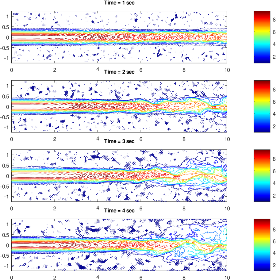
Figure 1. The velocity magnitude (m/s) at the elapsed time $t=1,2,3,4$ sec.

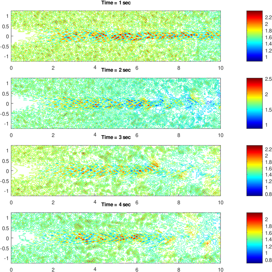
Figure 2. The density (kg/m³) at the elapsed time $t=1,2,3,4$ sec.

In Figure 2 we show the show the two-dimensional snapshots of the density, measured within the plane $z=0$ at elapsed times of 1, 2, 3 and 4 seconds. It is interesting that the most significant fluctuations of the density occur within the jet itself, and not in the turbulent flow around it (for example, compare the snapshots at $t=1$, where the jet is mostly intact throughout the length of the pipe, and at $t=4$, where the jet falls apart in the last third of the pipe). The fine “checkerboard” fluctuations on the spatial scale of the discretization above and below the jet appear to be an analog of the acoustic waves; indeed, combining the time-derivative of the density equation in (4.14) with the divergence of the momentum equation in (4.15) leads to

(5.4) $$\frac{\partial^{2}\rho}{\partial t^{2}}=\nabla^{2}:\Big{[}\Big{(}\frac{p_{0}}{2\rho_{sp}}\mathsfbi I+\boldsymbol{u}^{2}\Big{)}\rho\Big{]},$$

where the matrix which multiplies $\rho$ is obviously positive definite. The “speed of sound” here is, however, quite low (in comparison with the true acoustic waves) – observe that, for the given pressure and the density of the atom of argon, we have $p_{0}/2\rho_{sp}\sim 20$ m²/s², plus $\boldsymbol{u}^{2}$ contributes at most 100 m²/s², which yields about 10-11 m/s for the speed of such a wave in the given conditions. While one can probably devise numerical methods to suppress these “acoustic waves” by filtering out the appropriate spatial or temporal scales, here we leave them as they are, since they do not seem to significantly affect the turbulent dynamics of the jet in Figure 1.

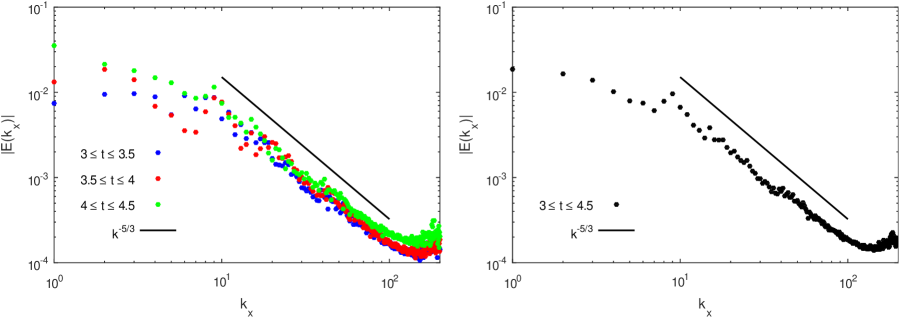
Figure 3. The Fourier spectra of the kinetic energy, averaged over different time intervals. The slope line $k^{-5/3}$ is given for the reference.

To verify that the behavior of the jet in Figure 1 indeed corresponds to the turbulent behavior observed in nature, in Figure 3 we show the time-averaged Fourier spectra of the kinetic energy of the flow. These spectra is computed as follows: first, the kinetic energy $E(\boldsymbol{x})=\|\boldsymbol{u}(\boldsymbol{x})\|^{2}/2$ is averaged over the cross-section of the pipe (thus becoming the function of the $x$-coordinate only). Then, the linear least-squares fit is subtracted from the result in the same manner as was done by Nastrom and Gage [26]; this is done to ensure that there is no sharp discontinuity between the energy values at the inlet and the outlet. Finally, the one-dimensional discrete Fourier transformation is applied to the result, so that the resulting Fourier transform of the kinetic energy, computed along the pipe, corresponds to the zero Fourier wavenumbers across the pipe. The subsequent time-averaging of the modulus of the Fourier transform is computed between $t=3$ and $t=4.5$ seconds of the elapsed time (that is, for the fully turbulent jet). On the left panel of Figure 3, we show the time averages computed for intervals $3\leq t\leq 3.5$ seconds, $3.4\leq t\leq 4$ seconds, and $4\leq t\leq 4.5$ seconds. On the right panel of Figure 3, we show the time average for the combined interval $3\leq t\leq 4.5$ seconds. As we can see, all plots align quite well with the $k^{-5/3}$ reference line, which indicates the Kolmogorov decay of the kinetic energy averages. Also, the plots are visually similar to the observations in the experimental work by Buchhave and Velte [11].

6. Summary

In the current work, we develop and test a fluid mechanical model for a macroscopic turbulent flow, which is triggered by a short range interaction potential. We start with a system of many identical particles, which interact via a short range potential. Applying the BBGKY formalism and a suitable closure, we obtain a Vlasov-type equation for the distribution density of a single particle with a mean field forcing. We show that the mean field forcing has an explicit and relatively simple form if the interaction potential corresponds to a hard sphere collision.

Next, for this Vlasov-type equation, we formulate the velocity moment hierarchy, similarly to how it is done in the conventional transition from kinetic theory to fluid mechanics. However, due to the fact that the mean field forcing replaces the conventional Boltzmann collision integral, the closure for the moment hierarchy differs from the one typically used in the conventional fluid mechanics; namely, we have to use the high Reynolds number condition for the closure instead of the Newton and Fourier laws. As a result, we arrive at a system of transport equations for the density, momentum and temperature, which is markedly different from the conventional Euler equations. First, the momentum equation in the new system has an additional forcing originating from the interaction potential, and, second, the new system preserves the pressure along the streamlines (while the conventional Euler equations preserve the entropy).

Finally, we numerically simulate the new equations in a realistic setting of argon flowing through a straight three-dimensional pipe. The laminar Bernoulli jet is chosen as an initial condition for the simulation, given that it is a steady state in the conventional Euler equations. Our simulation, however, shows that the laminar Bernoulli jet quickly develops into a fully turbulent flow, which visually resembles the observations in nature. We also confirm that the time averages of the kinetic energy of the simulated flow decay with the rate of negative five-third power of the Fourier wavenumber, which corresponds to the Kolmogorov spectrum.

Acknowledgment

This work was supported by the Simons Foundation grant #636144.

References

- Abramov [2017] R.V. Abramov. Diffusive Boltzmann equation, its fluid dynamics, Couette flow and Knudsen layers. Physica A, 484:532–557, 2017.
- Abramov [2019] R.V. Abramov. The random gas of hard spheres. J, 2(2):162–205, 2019.
- Abramov [2020] R.V. Abramov. Turbulent energy spectrum via an interaction potential. J. Nonlinear Sci., 30:3057–3087, 2020.
- Abramov [2021] R.V. Abramov. Formation of turbulence via an interaction potential. Preprint: https://arxiv.org/abs/2011.10042, 2021.
- Abramov and Otto [2018] R.V. Abramov and J.T. Otto. Nonequilibrium diffusive gas dynamics: Poiseuille microflow. Physica D, 371:13–27, 2018.
- Batchelor [2000] G.K. Batchelor. An Introduction to Fluid Dynamics. Cambridge University Press, New York, 2000.
- Bogoliubov [1946] N.N. Bogoliubov. Kinetic equations. J. Exp. Theor. Phys., 16(8):691–702, 1946.
- Boltzmann [1872] L. Boltzmann. Weitere Studien über das Wärmegleichgewicht unter Gasmolekülen. Sitz.-Ber. Kais. Akad. Wiss. (II), 66:275–370, 1872.
- Born and Green [1946] M. Born and H.S. Green. A general kinetic theory of liquids I: The molecular distribution functions. Proc. Roy. Soc. A, 188:10–18, 1946.
- Boublík [1986] T. Boublík. Background correlation functions in the hard sphere systems. Mol. Phys., 59(4):775–793, 1986.
- Buchhave and Velte [2017] P. Buchhave and C.M. Velte. Measurement of turbulent spatial structure and kinetic energy spectrum by exact temporal-to-spatial mapping. Phys. Fluids, 29(8):085109, 2017.
- Cercignani et al. [1994] C. Cercignani, R. Illner, and M. Pulvirenti. The mathematical theory of dilute gases. In Applied Mathematical Sciences, volume 106. Springer-Verlag, 1994.
- Chapman and Cowling [1991] S. Chapman and T.G. Cowling. The Mathematical Theory of Non-Uniform Gases. Cambridge Mathematical Library. Cambridge University Press, 3rd edition, 1991.
- Fermi [1927] E. Fermi. A statistical method for determining some properties of the atom. Rend. Accad. Naz. Lincei, 6:602–607, 1927.
- Golse [2005] F. Golse. The Boltzmann Equation and its Hydrodynamic Limits, volume 2 of Handbook of Differential Equations: Evolutionary Equations, chapter 3, pages 159–301. Elsevier, 2005.
- Grad [1949] H. Grad. On the kinetic theory of rarefied gases. Comm. Pure Appl. Math., 2(4):331–407, 1949.
- Greenshields et al. [2010] C.J. Greenshields, H.G. Weller, L. Gasparini, and J.M. Reese. Implementation of semi-discrete, non-staggered central schemes in a colocated, polyhedral, finite volume framework, for high-speed viscous flows. Int. J. Numer. Methods Fluids, 63(1):1–21, 2010.
- Hirschfelder et al. [1964] J.O. Hirschfelder, C.F. Curtiss, and R.B. Bird. The Molecular Theory of Gases and Liquids. Wiley, 1964.
- Kirkwood [1946] J.G. Kirkwood. The statistical mechanical theory of transport processes I: General theory. J. Chem. Phys., 14:180–201, 1946.
- Kolmogorov [1941a] A.N. Kolmogorov. Local structure of turbulence in an incompressible fluid at very high Reynolds numbers. Dokl. Akad. Nauk SSSR, 30:299–303, 1941a.
- Kolmogorov [1941b] A.N. Kolmogorov. Decay of isotropic turbulence in an incompressible viscous fluid. Dokl. Akad. Nauk SSSR, 31:538–541, 1941b.
- Kolmogorov [1941c] A.N. Kolmogorov. Energy dissipation in locally isotropic turbulence. Dokl. Akad. Nauk SSSR, 32:19–21, 1941c.
- Kullback and Leibler [1951] S. Kullback and R. Leibler. On information and sufficiency. Ann. Math. Stat., 22:79–86, 1951.
- Kurganov and Tadmor [2001] A. Kurganov and E. Tadmor. New high-resolution central schemes for nonlinear conservation laws and convection–diffusion equations. J. Comput. Phys., 160:241–282, 2001.
- Lennard-Jones [1924] J.E. Lennard-Jones. On the determination of molecular fields. – II. From the equation of state of a gas. Proc. R. Soc. Lond. A, 106(738):463–477, 1924.
- Nastrom and Gage [1985] G.D. Nastrom and K.S. Gage. A climatology of atmospheric wavenumber spectra of wind and temperature observed by commercial aircraft. J. Atmos. Sci., 42(9):950–960, 1985.
- Obukhov [1941] A.M. Obukhov. On the distribution of energy in the spectrum of a turbulent flow. Izv. Akad. Nauk SSSR Ser. Geogr. Geofiz., 5:453–466, 1941.
- Obukhov [1949] A.M. Obukhov. Structure of the temperature field in turbulent flow. Izv. Akad. Nauk SSSR Ser. Geogr. Geofiz., 13:58–69, 1949.
- Obukhov [1962] A.M. Obukhov. Some specific features of atmospheric turbulence. J. Geophys. Res., 67(8):3011–3014, 1962.
- Rényi [1961] A. Rényi. On measures of entropy and information. In Proceedings of the Fourth Berkeley Symposium on Mathematical Statistics and Probability, Volume 1: Contributions to the Theory of Statistics, pages 547–561, Berkeley, CA, 1961. University of California Press.
- Reynolds [1883] O. Reynolds. An experimental investigation of the circumstances which determine whether the motion of water shall be direct or sinuous, and of the law of resistance in parallel channels. Proc. R. Soc. Lond., 35(224–226):84–99, 1883.
- Struchtrup and Torrilhon [2003] H. Struchtrup and M. Torrilhon. Regularization of Grad’s 13-moment equations: Derivation and linear analysis. Phys. Fluids, 15:2668–2680, 2003.
- Thomas [1927] L.H. Thomas. The calculation of atomic fields. Proc. Camb. Phil. Soc., 23(5):542–548, 1927.
- van Leer [1974] B. van Leer. Towards the ultimate conservative difference scheme, II: Monotonicity and conservation combined in a second order scheme. J. Comput. Phys., 17:361–370, 1974.
- Vlasov [1938] A.A. Vlasov. On vibration properties of electron gas. J. Exp. Theor. Phys., 8(3):291, 1938.
- Weller et al. [1998] H.G. Weller, G. Tabor, H. Jasak, and C. Fureby. A tensorial approach to computational continuum mechanics using object-oriented techniques. Computers in Physics, 12(6):620–631, 1998.