A Quasipolynomial $(2+\varepsilon)$-Approximation for Planar Sparsest Cut

Abstract

The (non-uniform) sparsest cut problem is the following graph-partitioning problem: given a “supply” graph, and demands on pairs of vertices, delete some subset of supply edges to minimize the ratio of the supply edges cut to the total demand of the pairs separated by this deletion. Despite much effort, there are only a handful of nontrivial classes of supply graphs for which constant-factor approximations are known.

We consider the problem for planar graphs, and give a $(2+\varepsilon)$-approximation algorithm that runs in quasipolynomial time. Our approach defines a new structural decomposition of an optimal solution using a “patching” primitive. We combine this decomposition with a Sherali-Adams-style linear programming relaxation of the problem, which we then round. This should be compared with the polynomial-time approximation algorithm of Rao (1999), which uses the metric linear programming relaxation and $\ell_{1}$-embeddings, and achieves an $O(\sqrt{\log n})$-approximation in polynomial time.

1 Introduction

In the (non-uniform) sparsest cut problem, we are given a “supply” graph $G$ with an edge-cost function $\operatorname{cost}:E(G)\to\mathbb{R}_{\geq 0}$ and a demand function $\operatorname{demand}:V\times V\to\mathbb{R}_{\geq 0}$. For a nonempty proper subset $U$ of the vertices of $G$, the corresponding cut is the edge subset $\delta_{G}(U)=\{\{x,y\}\in E(G)\mid x\in U,y\not\in U\}$. The cost of this cut is $\operatorname{cost}(U):=\sum_{e\in\delta_{G}(U)}\operatorname{cost}(e)$, and the demand separated by it is $\operatorname{demand}(U):=\sum_{\{u,v\}:|\{u,v\}\cap U|=1}\operatorname{demand}(u,v)$. The sparsity of the cut given by $U$ is $\Phi(U):=\operatorname{cost}(U)/\operatorname{demand}(U)$. The goal is to find a set $U$ that achieves the minimum sparsity of this instance, defined as:

$$\Phi^{*}:=\min_{U:U\neq\emptyset,V(G)}\Phi(U)=\min_{U:U\neq\emptyset,V(G)}\frac{\operatorname{cost}(U)}{\operatorname{demand}(U)}.$$ (1)

(The special case with unit demand between every pair of vertices is called the uniform sparsest cut, discussed in §1.1.) Finding sparse cuts is a natural clustering and graph decomposition subroutine used by divide-and-conquer algorithms for graph problems, and hence has been widely studied.

The problem is NP-hard [MS90], and so the focus has been on the design of approximation algorithms. This line of work started with an $O(\log D\log C)$-approximation given by Agrawal, Klein, Rao, and Ravi [KRAR95, KARR90], where $D$ is the sum of demands and $C$ the sum of capacities. After a several developments, the best approximation factor currently known is $O(\sqrt{\log n}\log\log n)$ due to Arora, Lee, and Naor [ALN08]. Moreover, the problem is inapproximable to any constant factor, assuming the unique games conjecture [CKK⁺06, KV15].

Given this significant roadblock for general graphs, a major research effort has sought $O(1)$-approximation algorithms for “interesting” classes of graphs. In particular, the problem restricted to the case where $G$ is planar has received much attention over the years. The best approximation bound for this special case before the current work remains the $O(\sqrt{\log n})$-approximation of Rao [Rao99], whereas the best hardness result merely rules out a $\frac{1}{0.878+\varepsilon}\approx(1.139-\varepsilon)$-approximation assuming the unique games conjecture [GTW13]. One source of the difficulty is that the “demand” graph, i.e., the support of the demand function, is not necessarily planar. Indeed, the hardness results are obtained by embedding general instances of max-cut in this demand graph.

The sparsest cut problem has been studied on even more specialized classes of graphs in order to gain insights for the planar case: see, e.g., [OS81, GNRS04, CGN⁺06, CJLV08, CSW13, LR10, CFW12]. Again, despite successes on those specialized classes (see §1.1 for a discussion), getting a constant-factor approximation for non-uniform sparsest-cut on arbitrary planar graphs has remained open so far. Our main result is such an algorithm, at the expense of quasi-polynomial runtime:

Theorem 1.1 (Main Theorem).

There is a randomized algorithm for the non-uniform sparsest cut problem on planar graphs which achieves a $(2+\varepsilon)$-approximation in quasi-polynomial time $O(n^{\log^{2}n/\operatorname{poly}(\varepsilon)})$.

1.1 Related Work

The sparsest cut problem is NP-hard, even for the uniform case [MS90]. The initial approximation factor of $O(\log D\log C)$ [KRAR95, KARR90], where $D$ is the sum of demands and $C$ the sum of capacities, was improved to $O(\log^{2}n)$ [PT95], to $O(\log n)$ [LLR95, AR98], $O(\log^{3/4}n)$ [CGR08], and finally to the current best $O(\sqrt{\log n}\log\log n)$ [ALN08].

Many special classes of graphs admit constant-factor approximations for non-uniform sparsest cut. These include outerplanar [OS81], series-parallel [GNRS04, CSW13, LR10], $k$-outerplanar graphs [CGN⁺06], graphs obtained by $2$-sums of $K_{4}$ [CJLV08], graphs with constant pathwidth and related families [LS09, LS13], and bounded treewidth graphs [CKR10, GTW13]. Most of these approximations are with respect to the “metric” relaxation LP, via $\ell_{1}$-embeddings [LLR95]. The bounded treewidth results are exceptions: they use a stronger LP, and it remains open whether the metric relaxation has a constant integrality gap even for graphs of treewidth $3$, which are also planar. Neither our result, nor the results of [CKR10, GTW13], shed light on this question. A “meta-result” of Lee and Sidiropoulos [LS09] proves that if planar graphs embed into $\ell_{1}$ with constant distortion, and if constant-distortion $\ell_{1}$-embeddability is closed under clique-sums, then all minor-closed families have constant-factor approximations with respect to the standard LP.

Uniform Version. For the uniform version of sparsest cut, $O(1)$-approximations exist for classes of graphs that exclude non-trivial minors, via low-diameter decompositions [KPR93]. Park and Philips [PP93] solve the uniform problem on planar graphs in $O(n^{3})$ time; see Abboud et al. [ACAK20] for a speedup. Abboud et al. [ACAK20] give an $O(1)$-approximation in near-linear time, improving upon the near-linear time $O(\log n)$-approximation of Rao [Rao92]. Finally, Patel [Pat13] showed that the uniform sparsest-cut problem can be exactly solved in time $n^{O(g)}$ for graphs that embed into a surface of genus at most $g$. The approximation factor for the uniform problem on general graphs has been improved from $O(\log n)$ [LR10] by rounding LP relaxations, to $O(\sqrt{\log n})$ [ARV09] by rounding SDP relaxations.

Integrality Gaps for the Basic LP: There are many results on lower bounds and limitations to known techniques; see, e.g., works by Khot and Vishnoi [KV15], Chawla et al. [CKK⁺06], Lee and Naor [LN06], and others. Naor and Young [NY17, NY18] show lower bounds on integrality gap of the semidefinite program for sparsest-cut that almost match the upper bounds of [ALN08].

Hardness of Approximation: an $\alpha$-approximation to non-uniform sparsest cut on series-parallel (i.e., treewidth-$2$) graphs, which are also planar, gives an $(1/\alpha)$-approximation to the MaxCut problem [GTW13]. The results of [Hås01, KKMO07] now imply that sparsest cut is hard to approximate better than $\frac{17}{16}$ unless P=NP, and to better than $1/0.878$ assuming the Unique Games conjecture. It is known that for every $\varepsilon>0$, there are graph families with treewidth $f(\varepsilon)$ on which sparsest-cut is hard to approximate better than a factor of $(2-\varepsilon)$, assuming the Unique games conjecture—but these hard instances are not known to be planar [GTW13].

1.2 Techniques

We outline the main conceptual steps of our algorithm, and some intuition for why these are needed:

1. Duality. One advantage of planar instances is the duality between cuts and cycles. Indeed, there is an optimal solution that corresponds to a simple cycle $C_{0}$ in the dual graph $G^{*}$. So it suffices to find some cycle in the dual with low total edge-cost, that separates a lot of demand (which is now between pairs of faces), see Proposition 2.2.

2. Low-Complexity Clusterings. Suppose we efficiently find a hierarchical partition of the dual into subgraphs called clusters, such that whenever some cluster $K$ splits into subclusters $K_{1},K_{2},\ldots K_{t}$, the cycle $C_{0}$ crosses between these subclusters at most $O(\log n)$ times. (I.e., $C_{0}$ has “low complexity” with respect to the partition.) Then, we can find a $2$-approximation to the sparsest “low-complexity” solution using a linear program, as described in Item 7 below.

3. Finding these Low-Complexity Clusterings. How do we find such a good hierarchical decomposition? We repeatedly find low-diameter decompositions with decreasing radii. If the cost of the edges of $C_{0}$ that lies within each cluster $K$ is at most $O(\varepsilon^{-1}\log n)$ times the diameter of $K$, then performing a low-diameter decomposition of $K$ causes only $O(\varepsilon^{-1}\log n)$ edges to be cut in expectation. I.e., the expected number of times $C_{0}$ crosses between subclusters of $K$ is small, as desired. (Observe we get a small number of crossings only in expectation: we’ll come back to this in Item 6).

4. Patching. However, the cost of $C_{0}$ within some cluster $K$ may exceed $\Theta(\varepsilon^{-1}\log n)$ times the cluster diameter. In this case we patch the cycle, adding some collection of shortest paths within the cluster $K$, that locally break this cycle into several smaller cycles. We elaborate on this operation in the paragraphs following this outline. If we imagine maintaining a collection of cycles, starting with the single cycle $C_{0}$, the patching replaces one cycle in this collection by many. Moreover the cost of this collection increases by a factor of at most $(1+\varepsilon/\log n)$ in each level of the recursion.

5. Controlling the Cost. Since the ratio of the largest to the smallest edge cost can be assumed to be polynomially bounded (see Section 2) and the diameter decreases by a factor of $2$ at each level of the decomposition, there are $O(\log n)$ levels of recursion. This means the total increase in the cost of the entire collection of cycles is at most $(1+\varepsilon/\log n)^{O(\log n)}=(1+O(\varepsilon))$. So the sparsest simple cycle from this collection (and its corresponding simple cut in the primal) has sparsity at most $(1+O(\varepsilon))$ times the optimal sparsity.

6. “Non-Deterministic” Hierarchical Decompositions. Recall, in Item 3 we ensured the low-complexity property only in expectation. We need it to hold for all the clusters of the decomposition, and so with high probability for a single cluster. To achieve this we choose $\Theta(\log n)$ independent low-diameter decompositions for each cluster, and apply the procedure recursively to each part of each partition. This is reminiscent of an idea introduced by Bartal et al. [BGK16]. It ensures that one of these partitions has low complexity, with high probability. We call this a non-deterministic hierarchical decomposition, and show that it has total size $n^{O(\varepsilon^{-1}\log n)}$.

7. The Linear Program. All the above steps were part of the structure lemma. They show the existence (whp.) of a near-optimal low-complexity solution with respect to the non-deterministic hierarchical decomposition. It now remains to select one of the decompositions at each level, and to find this cycle that has low complexity with respect to this restricted decomposition tree. To do this, we write a linear program, and round it. The high level ideas are similar to those used for the sparsest-cut problem on bounded-treewidth graphs, and we elaborate on these in the paragraph below.

Before we proceed, a caveat: the actual algorithm differs from the above outline in small but important details; e.g., we coarsen the low-diameter decompositions to ensure that each partition has few parts, which means the diameter of our clusters does not necessarily drop geometrically. Since these details would complicate the above description, we introduce them only when needed.

We now give more details about two of the key pieces: the patching lemma, and the linear program.

1.2.1 A Patching Lemma for Planar Graphs

An important ingredient of our approach is a patching lemma for non-uniform sparsest cut in planar graphs. As with most patching lemmas, our patching lemma (and the associated patching procedure) are only used for the analysis of our algorithm; Their goal is to help exhibit a near-optimum solution that is “well-structured”. There are some similarities to the patching lemmas of Arora [Aro97] and Bartal et al. [BGK16] for the Traveling Salesman Problem (TSP) in Euclidean space and doubling metrics respectively, but there are some important differences. Given a cluster $K$ of diameter $D$ and a given cycle $C$ (thought of as the optimum solution), the goal of our patching procedure is to break $C$ into a collection of cycles such that (1) for each demand pair separated by $C$, there is a cycle in the collection separating that pair; (2) for each cycle $C^{\prime}$ in the collection, the total cost of the edges of $C^{\prime}$ inside cluster $c$ is $O(\varepsilon^{-1}\log n)$; and (3) the total cost of the edges of the cycles of the collection inside cluster $c$ is at most $(1+\varepsilon/\log n)$ times the total cost of the edges of cycle $C$ inside $K$. We explain our patching procedure in Figure 1; please read the captions to follow along.

(a) The original cycle $C$ in black, and the cluster $K$ in dashed red. The three black dots are vertices on the optimal solution such that the edge-cost of the optimal solution $C$ within $K$ between any two consecutive dots is $\Theta(\frac{\log n}{\varepsilon}D)$, where $D$ is the diameter of $K$.

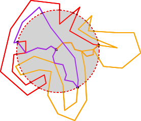
(b) Since the cost of $C$ within $K$ between consecutive black dots is $\Theta(\varepsilon^{-1}\log n)$ times the diameter of $K$, adding the shortest paths (shown in blue) from some root node $r$ to the dots on $C$ only increases the cost by a factor of $(1+\nicefrac{{\varepsilon}}{{\log n}})$.

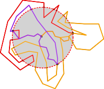
Figure 1: The addition of these paths splits the original tour into three tours (possibly self-intersecting), shown in purple, orange, and red. One of these three tours achieves sparsity at most that of the original tour (up to a $(1+\nicefrac{{\varepsilon}}{{\log n}})$ factor). Importantly, the cost within $K$ of this good tour is $O(\frac{\log n}{\varepsilon}D)$, by construction, which is proportional to the diameter of the cluster. Repeating this argument recursively, and using that we have $O(\log n)$ levels, the total error is bounded by a multiplicative factor of $(1+\varepsilon)$.

Obtaining a patching lemma for a planar problem seems surprising to us. While low-diameter decompositions have been widely used to obtain approximation schemes for problems in Euclidean spaces of constant dimension (e.g., for the traveling salesman problem, or facility location), it was unclear how to use low-diameter decompositions effectively to obtain approximation schemes for these problems on planar graphs. One hurdle in applying this technique to planar graphs has been that that the isoperimetric inequality does not hold, and so the cost of the edges of the cluster boundary cannot be related to the diameter of the cluster. Without isoperimetry, there are examples where forcing the optimum solution to make a small number of crossings between child clusters (through portals, for example) incurs a huge increase in cost. One could get a coarser control on the problem structure, e.g., by bounding the diameter, which gave constant-factor approximations for related problems such as multicut or $0$-extension, but only an $O(\sqrt{\log n})$-approximation for sparsest cut. The approach of enriching the optimum circumvents this issue for the non-uniform sparsest cut problem.

1.2.2 A Linear Program over these Clusterings

While the natural candidate for finding the best solution over a non-deterministic hierarchical decomposition would be a dynamic program, we currently do not know how to get a good approximation for sparsest cut using dynamic programming, even for simpler graph classes such as treewidth-$2$ graphs. However, we can use linear programs as in [CKR10, GTW13]: we add linear constraints capturing that the LP has to “choose” one of the $\Theta(\log n)$ potential sub-partitionings at each level of the decomposition. Our linear program has variables that capture all the “low-complexity” partial solutions within each cluster, and constraints that ensure the consistency of the solution and of the partitioning over all $O(\log n)$ levels of the entire decomposition. The details appear in §5.

2 Notation and Preliminaries

Let $[n]$ denote $\{1,\ldots,n\}$. Given an instance of non-uniform sparsest-cut, the following lemma allows us to restrict edge costs and demands on the pairs to be integers in a bounded range. It is proved in §A.3.

Lemma 2.1.

An $\alpha$-approximation algorithm $\mathcal{A}$ with runtime $T_{n}$ for sparsest cut instances on $n$-vertex planar graphs with the edge costs in $[n^{2}]$ and demands for pairs in $[n^{3}]$ implies an $(1+o(1))\alpha$-approximation algorithm with running time $O(n^{3}\cdot T_{n})$ for planar sparsest cut instances with arbitrary non-negative edge costs and demands.

For a connected graph $G$ and subset $U\subseteq V(G)$ of vertices, let $\delta_{G}(U)$ denote the set of edges $e$ of $G$ such that $U$ contains exactly one endpoint of $e$. A set of edges of this form is called a cut. We drop the subscript when the graph $G$ is unambiguous. Let $G[U]$ denote the subgraph induced by $U$. A nonempty proper cut $\delta_{G}(U)$ is called a bond or a simple cut if both induced subgraphs $G[U]$ and $G[V(G)\setminus U]$ are connected. The following simple result from, e.g., [OS81] is proved in §A.3.

Proposition 2.2.

The optimal sparsity in (1) can be achieved by a set $U$ such that $\delta_{G}(U)$ is a simple cut.

Planar duality

We work with a connected planar embedded graph, a graph $G=(V,E)$ together with an embedding of $G$ in the plane. There is a corresponding planar embedded graph $G^{*}$, the planar dual of $G$. The vertices of the dual are the faces of $G$, and the faces of the dual are the vertices of $G$. The edges in the dual correspond one-to-one with the edges in $G$, and we identify each edge in the dual $G^{*}$ with the corresponding edge in $G$, and hence having the same cost. The demand function can be considered as mapping pairs of faces in $G^{*}$ to non-negative integers.

Proposition 2.3 (Simple Cycle (e.g., [KM], Ch. 5)).

Let $G$ be a connected planar embedded graph, and let $G^{*}$ be its dual. A set of edges forms a simple cut $\delta_{G}(U)$ in $G$ if and only if the edges form a simple cycle $C$ in $G^{*}$.

Fix a face $f_{\infty}$ of $G^{*}$, i.e., a vertex of $G$. Think of it as the infinite face of $G^{*}$. Let $C$ be a simple cycle in $G^{*}$. By Proposition 2.3, the edges of $C$ are the edges of some simple cut $\delta_{G}(U)$ where $U$ is a set of vertices of $G$ such that $f_{\infty}$ is not in $U$. We define the set of faces enclosed by $C$ to be $U$, and we denote this set of faces by $U(C)$.

In view of Propositions 2.2 and 2.3, seeking a sparsest cut in a planar embedded graph is equivalent to seeking a simple cycle $C$ in $G^{*}$ with the objective

$$\min\frac{\text{cost of edges of }C}{\sum\{\operatorname{demand}(\{f_{1},f_{2}\})\mid f_{1}\text{ enclosed by }C,f_{2}\text{ not enclosed by }C\}}$$ (2)

Indeed, the value of the objective (2) is the sparsity of $U(C)$ as defined in the introduction.

Lemma 2.4.

Suppose $C$ is a simple cycle in $G^{*}$. Let $C_{1},\ldots,C_{k}$ be cycles such that each edge occurs an odd number of times in $C_{1},\ldots,C_{k}$ iff it appears in $C$. Then, for each pair $x,y$ of vertices of $G$, if $x$ and $y$ are separated by $C$ then they are separated by some $C_{i}$.

Lemma 2.5.

Suppose $C_{0}$ is a simple cycle in $G^{*}$ such that $U(C_{0})$ has sparsity $s$. Let $C_{1},\ldots,C_{k}$ be simple cycles such that every demand separated by $C_{0}$ is separated by at least one of $C_{1},\ldots,C_{k}$. Suppose the total cost of edges in $C_{1},\ldots,C_{k}$ (counting multiplicity) is at most $1+\varepsilon$ times the cost of edges in $C_{0}$. Then there is some cycle $C_{i}$ such that $U(C_{i})$ has sparsity at most $(1+\varepsilon)s$.

Low-Diameter Decompositions and $D$-Bounded Partitions.

A low-diameter decomposition scheme takes a graph and randomly breaks it into components of “bounded” (strong) diameter, so that the probability of any edge being cut is small. Concretely, let $H$ be a graph with edge costs $\operatorname{cost}(e)\geq 0$. Let $\operatorname{dist}_{H}(x,y)$ be the shortest-path distances according to these costs. The (strong) diameter of a subset $U\subseteq V(H)$ is the maximum distance between any two nodes in $U$, measured according to $\operatorname{dist}_{H[U]}(\cdot,\cdot)$, the distances within this induced subgraph $H[U]$. The strong diameter of a partition $\mathcal{P}=\{V_{1},V_{2},\ldots,V_{s}\}$ of the vertex set $V(H)$ is the maximum strong diameter of any of its parts. A partition is $D$-bounded if it has strong diameter at most $D$. The next claim follows from [AGMW10, Theorem 3],[AGG⁺19, Theorem 4]:

Theorem 2.6.

There exists a constant $\beta>0$ such that given any undirected weighted planar graph $H$ and parameter $D>0$, there exists a distribution $\Pi$ over $D$-bounded vertex partitions such that

$$\Pr[\text{$u,v$ fall in different components}]\leq\beta\;\frac{\operatorname{cost}(\{u,v\})}{D}$$

for any edge $uv\in E(H)$. Moreover, this distribution is sampleable in polynomial time.

3 Nondeterministic Clustering

Recall that the input to our algorithm is:

• a connected simple planar embedded graph $G=(V,E)$ on $n$ vertices and $O(n)$ edges,

• assignments of edge costs $\operatorname{cost}:E\to[n^{2}]$, and demands $D:{V\choose 2}\to[n^{3}]$ to vertex pairs, and

• a parameter $\varepsilon\in[0,1]$.

We want the algorithm to output a cut with sparsity $2(1+O(\varepsilon))$ times the optimal sparsity. By Proposition 2.3 we can assume that the optimal cut corresponds to a simple cycle in the planar dual $G^{*}$. In what follows, we focus on the dual graph $G^{*}$; the algorithm will select such a simple cycle. We interpret $\operatorname{cost}(\cdot)$ as an assignment of costs to the edges of $G^{*}$.

The algorithm consists of two phases. Ideally, the first phase would construct a hierarchical clustering of $G^{*}$ such that there exists a near-optimal solution $C^{*}$ that crosses each cluster at most $Z$ times, where $Z$ is polylogarithmic. Given the existence of this “low-complexity” solution, the second phase would then use this clustering to compute some near-optimal solution. We proceed slightly differently: Our method’s first phase instead constructs a nondeterministic hierarchical clustering (NDHC) of $G^{*}$, which represents a large family of hierarchical clusterings. Fortunately, our second phase can be adapted to work with this family.

Specifically, our algorithm applies a randomized partitioning scheme to each cluster in each level of hierarchy to form subclusters. However, this partitioning scheme just ensures that the “low-complexity” property for each partition in expectation. This is not good enough because there are many clusters being partitioned, so some of the partititions might not be good. To handle this shortcoming, the procedure produces $t\approx n^{O(\log n)}$ partitions of each cluster into subclusters, so that one of these partitions is good with high probability. Since we do not know the target solution $C^{*}$, we cannot choose among the $t$ partitions. Instead we produce a representation of all the choices using an NDHC. A similar idea of repeating the clustering was previously used by Bartal, Gottlieb, and Krauthgamer [BGK16] and in subsequent papers in the context of the TSP on doubling metrics.

3.1 Definitions

Definition 3.1 (Nondeterministic Hierarchical Clustering).

For $t\in\mathbb{Z}_{+}$, a $t$-nondeterministic hierarchical clustering ($t$-NDHC) for $G^{*}$ is a rooted tree $\mathcal{T}$ with alternating levels of cluster nodes and partition nodes:

• A cluster node $c$ corresponds to a set $K(c)$ of vertices of $G^{*}$, called a cluster. Each nonleaf cluster node has at most $t$ partition nodes as its children.

• A partition node $p$ with parent $c$ corresponds to a partition $\pi(p)$ of the vertex set $K(c)$. The node $p$ has a child $c^{\prime}$ for each part $P\in\pi(p)$, where $c^{\prime}$ is a cluster node with $K(c^{\prime})=P$.

• The root of $\mathcal{T}$ is a partition node which corresponds to the trivial partition where all vertices of the graph are in a single part; hence it has a single cluster node as its child.

• Each leaf is a cluster node with a singleton cluster.

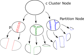
Figure 2: A fragment of tree $\mathcal{T}$ showing cluster and partition nodes.

Contrast this structure with a hierarchical partition used in the literature, which is usually represented by a tree where each node represents both a cluster (a subset $K(c)$ of vertices of $G^{*}$), and a partition of this cluster $K(c)$ into clusters represented by its children. (In that sense, each node in such a tree is both a cluster node and a partition node.) We consider several independent partitions of the same cluster, so we tease these two roles apart. The usual definition of hierarchical partition corresponds to the case where $t=1$. We refer to a $1$-NDHC as an ordinary hierarchical clustering.

Definition 3.2 (Normal and Shattering Partition Nodes).

A partition node is called shattering if its children cluster nodes are all leaves, and is otherwise called normal.

Definition 3.3 (Part Arity).

The part arity of $\mathcal{T}$ is the maximum number of children of any normal partition node $p$ (which is the same as the maximum number of parts in any of the partitions corresponding to these nodes). We do not limit the number of children of a shattering partition node.

Definition 3.4 (Forcing and Relevance).

Given a $t$-NDHC $\mathcal{T}$ with $t>1$, define a forcing of $\mathcal{T}$ to be a partial function $\varphi$ from cluster nodes to partition nodes such that, for each nonleaf cluster node $c$, (1) if $\varphi(c)$ is defined then $\varphi(c)$ is a child of $c$ and (2) if every partition node ancestor of $c$ is in the image of $\varphi$ then $\varphi(c)$ is defined.

We denote by $\mathcal{T}|_{\varphi}$ the ordinary hierarchical decomposition obtaining by retaining only partition nodes $p$ that are in the image of $\varphi$ (and also the partition node that is the root of $\mathcal{T}$).

Definition 3.5 (Internal and Crossing Edges).

An edge of $G^{*}$ is internal to a set $K$ of vertices if both endpoints belong to $K$. For a partition $\pi$ of a subset of the vertices of $G^{*}$, we say an edge crosses $\pi$ if the two endpoints of the edge lie in two different parts of $\pi$. (This requires that the edge be internal to the subset.) We use $\delta_{G^{*}}(\pi)$ to denote the set of edges crossing $\pi$.

Finally, we define the notion of amenability, which captures the property of a candidate cycle $C$ having “low complexity” with respect to a partition node. Friendliness is the same notion, but for a near-optimal cycle and an entire NDHC.

Definition 3.6 (Amenability).

For a nonnegative integer $Z$, a cycle $C$ of $G^{*}$ is $Z$-amenable for a partition node $p$ if at most $Z$ of its edges cross $\pi(p)$. The cycle $C$ is $Z$-amenable for an (ordinary) hierarchical clustering $\mathcal{T}$ if it is $Z$-amenable for every partition node $p$ in $\mathcal{T}$.

Definition 3.7 (Friendly $\mathcal{T}$).

For a nonnegative integer $Z$, and $\varepsilon>0$, a $t$-nondeterministic hierarchical clustering $\mathcal{T}$ of $G^{*}$ is $(Z,\varepsilon)$-friendly if there exists a cycle $\widehat{C}$ in $G^{*}$ such that:

• $\widehat{C}$ has sparsity at most $1+\varepsilon$ times the optimal sparsity for the entire input graph;

• There exists a forcing $\varphi$ of $\mathcal{T}$ such that $\widehat{C}$ is $Z$-amenable with respect to ${\mathcal{T}|}_{\varphi}$.

3.2 Constructing a Hierarchical Clustering

We now give a procedure $\mathcal{A}$ that takes integers $t$ and $Z$, and constructs a $t$-nondeterministic hierarchical clustering $\mathcal{T}$ of part arity $2Z$ and depth $O(\log n)$ and such that each leaf is a cluster node $c$ such that $|K(c)|=1$. In the next section, we show that there is a value of $Z$ that is $O(\log n)$ and a value of $t$ that is $n^{O(\text{polylog }n)}$ for which $\mathcal{T}$ is $(Z,\varepsilon)$-friendly with probability at least $1-\nicefrac{{1}}{{n}}$.

The level $\ell$ of a cluster node $c$ (or partition node $p$) in $\mathcal{T}$ is the number of cluster nodes (or partition nodes) on the path from the root to $c$ in $\mathcal{T}$, not including $c$ (or $p$). Thus the root and its child have level 0, its grandchildren and great-grandchildren have level 1, and so on. Define

$$\Delta_{\ell}:=\operatorname{diameter}(G^{*})/2^{\ell}.$$ (3)

The procedure $\mathcal{A}$ is specified in Algorithm 1. (We later choose the constant $a$ used in it.) At a high level, it builds $\mathcal{T}$ top-down. The root is a partition node with a single part containing all the vertices and with a single child, a cluster node whose cluster consists of all the vertices. The procedure iteratively adds levels to $\mathcal{T}$. For each cluster node $c$ at the current level $\ell$, it randomly selects $O(\log n)$ independent $\Delta_{\ell+1}$-bounded partitions. For each of these partitions, it considers all possible choices of $2Z$ parts, and merges the remaining parts with adjacent chosen parts. (The merging procedure is given in Algorithm 2; note that the merges may cause the diameter of the parts to increase.) The children of cluster node $c$ are the partition nodes corresponding to these partially-merged partitions; the children of a partition node $p$ correspond to the parts of the partition $p$. This process stops when $\ell=\lceil\log\operatorname{diameter}(G^{*})\rceil$, whereupon each non-singleton cluster is shattered into singleton nodes. Note the two unusual parts to this construction: the use of multiple partitions for each cluster (which makes it a nondeterministic partition), and the merging of parts (which bounds the part arity by $2Z$, at the cost of increasing the cluster diameter).

0.1 init: $\mathcal{T}\leftarrow$ root partition node $p$ with $\pi(p)=\{V(G^{*})\}$, and child $c$ with $K(c)=V(G^{*})$;

0.2 for $\ell=0,1,\ldots,\lceil\log\operatorname{diameter}(G^{*})\rceil$ do

0.3       foreach cluster node $c$ at level $\ell$ with $|K(c)|>1$ do

0.4             for $i=1,\ldots,a\log n$ do

0.5                   $\pi_{i}\leftarrow$ independent random $\Delta_{\ell+1}$-bounded partition of $K(c)$ ;

0.6                   foreach subset $\kappa\neq\emptyset$ of at most $2Z$ parts of $\pi_{i}$ do

0.7                         $\pi_{i,\kappa}\leftarrow$ MergeParts$(\pi_{i},\kappa)$ ;

0.8                         create a child partition node $p_{i,\kappa}$ of $c$ with $\pi(p_{i,\kappa})=\pi_{i,\kappa}$;

0.9                         foreach part $K$ of $\pi(p_{i,\kappa})$ do

0.10                               create a child cluster node $c^{\prime}$ of $p_{i,\kappa}$ with $K(c^{\prime})=K$;

0.11                              

0.12                        

0.13                  

0.14            

0.15      

0.16foreach leaf cluster node $c$ with $|K(c)|>1$ do

0.17       let $c$ have a single child partition node $p$ which shatters $K(c)$: $\pi(p):=\{\{v\}\mid v\in K(c)\}$;

0.18       let $p$ have a child cluster node $c_{v}$ for each node $v\in K(c)$, having $K(c_{v}):=\{v\}$ ;

0.19      

Algorithm 1 Procedure $\mathcal{A}$ to construct the $t$-NDHC with part arity $Z$

0.1 $\pi^{\prime}\leftarrow\pi$ ;

0.2 while $\exists$ edge $uv$ such that the part of $\pi^{\prime}$ containing $u$ intersects $\kappa$ and the part containing $v$ does not intersect $\kappa$ do

0.3       merge the two parts

return $\pi^{\prime}$

Algorithm 2 MergeParts$(\pi,\kappa)$

Lemma 3.8 (Properties I).

The $t$-nondeterministic hierarchical clustering $\mathcal{T}$ of the dual graph $G^{*}$ produced by Algorithm 1 has $t=n^{O(Z)}$, depth $O(\log n)$, part arity at most $2Z$, and total size $n^{O(Z\log n)}$.

Proof.

The loops in Algorithms 1 and 1 iterate over $a\log n$ and $n^{2Z}$ values respectively; the value of $t$ is at most their product. The part arity follows from the fact that each partition $\pi_{i,\kappa}$ has at most $2Z$ parts. The depth of $\mathcal{T}$ is at most $O(\log\operatorname{diameter}(G^{*}))=O(\log n)$, thanks to Lemma 2.1. Hence the total size of $\mathcal{T}$ is at most $(a\log n\cdot n^{2Z}\cdot Z)^{\text{depth}}=n^{O(Z\log n)}$. ∎

In §4, we prove that there is a choice of $Z$ with $Z=O(\log n/\varepsilon)$ for which $\mathcal{T}$ is $(Z,\varepsilon)$-friendly with high probability. In §5 we show how to write and round a linear program to find an approximate sparsest cut, given a $(Z,\varepsilon)$-friendly $t$-NDHC $\mathcal{T}$.

4 The Structure Theorem

Before proceeding with the description of the algorithm, we state and prove the structure theorem.

Theorem 4.1.

There is a choice of $Z$ that is $O(\log n/\varepsilon)$ for which the NDHC produced by procedure $\mathcal{A}$ is a $(Z,\varepsilon)$-friendly with probability at least $1-\nicefrac{{1}}{{n}}$.

To prove Theorem 4.1, we describe and analyze a virtual procedure $\mathcal{V}$ given in Algorithm 3 which performs the steps from the actual procedure $\mathcal{A}$, plus some extra virtual steps in the background for the purpose of the analysis. It takes as input not only the graph $G^{*}$ but also a cycle $C_{0}$ with optimal sparsity (which the algorithm $\mathcal{A}$ does not have). The procedure might fail but we show that failure occurs with probability at most $1/n$. Assuming no failures, it produces not only $\mathcal{T}$ but also a polynomial-size set $\mathcal{C}$ of cycles such that

• for each cycle $C\in\mathcal{C}$, there is a forcing $\varphi$ of $\mathcal{T}$ such that $C$ is $Z$-amenable with respect to ${\mathcal{T}|}_{\varphi}$.

• The total cost of cycles in $\mathcal{C}$ is at most $1+\varepsilon$ times the cost of $C_{0}$.

• Every two faces of $G^{*}$ separated by $C_{0}$ are separated by some cycle in $\mathcal{C}$.

Lemma 2.5 then implies that there is a cycle $\widehat{C}$ whose sparsity is at most $1+\varepsilon$ times optimal and that is $Z$-amenable with respect to ${\mathcal{T}|}_{\varphi}$ for some forcing $\varphi$ of $\mathcal{T}$. Again, we emphasize that the virtual procedure $\mathcal{V}$ is merely a thought experiment for the analysis. The lines added to $\mathcal{A}$ are highlighted for convenience. We now outline $\mathcal{V}$, and state the lemmas that prove Theorem 4.1. We then prove these lemmas in §4.3.

4.1 The Virtual Procedure $\mathcal{V}$

0.1 init: $\mathcal{T}\leftarrow$ root partition node $p$ with $\pi(p)=\{V(G^{*})\}$, and child $c$ with $K(c)=V(G^{*})$;

0.2   init: $\mathcal{C}\leftarrow\{C_{0}\}$, $\psi[\cdot,\cdot]\leftarrow$ an empty table ;

0.3 for $\ell=0,1,\ldots,\lceil\log\operatorname{diameter}(G^{*})\rceil$ do

0.4       foreach cluster node $c$ at level $\ell$ with $|K(c)|>1$ do

0.5               foreach cycle $C\in\mathcal{C}$ valid for cluster $c$ do  $\mathcal{C}\leftarrow(\mathcal{C}\setminus\{C\})\,\cup$ Patch$(C,c,\Delta_{\ell})$;

0.6             for $i=1,\ldots,a\log n$ do

0.7                   $\pi_{i}\leftarrow$ random $\Delta_{\ell+1}$-bounded partition of $K(c)$ ;

0.8                   foreach subset $\kappa\neq\emptyset$ of at most $2Z$ parts of $\pi_{i}$ do

0.9                         $\pi_{i,\kappa}\leftarrow$ MergeParts$(\pi_{i},\kappa)$ ;

0.10                         create a child partition node $p_{i,\kappa}$ of $c$ with $\pi(p_{i,\kappa})=\pi_{i,\kappa}$ ;

0.11                         foreach part $K$ of $\pi(p_{i,\kappa})$ do

0.12                               create a child cluster node $c^{\prime}$ of $p_{i,\kappa}$ with $K(c^{\prime})=K$;

0.13                              

0.14                        

0.15                  

0.16              foreach cycle $C\in\mathcal{C}$ that is valid for cluster node $c$ do

0.17                     if $|\{e\in C\mid e\text{ crosses }\pi_{i}\}|>Z$ for all $i\in[a\log n]$ then fail;

0.18                     $i\leftarrow$ any index in $[a\log n]$ s.t.  $|\{e\in C\mid e\text{ crosses }\pi_{i}\}|\leq Z$ ;

0.19                     $\kappa\leftarrow\{P\in\pi_{i}\mid P$ contains an endpoint of an edge of $C$ internal to $K(c)\}$ ;

0.20                     if $\kappa=\emptyset$ then $\kappa\leftarrow\{P\}$ where $P$ is chosen arbitrarily from $\pi_{i}$;

0.21                     $\psi[c,C]\leftarrow p_{i,\kappa}$ ;

0.22                  

0.23            

0.24      

0.25foreach leaf cluster node $c$ with $|K(c)|>1$ do

0.26       let $c$ have a single child partition node $p$ which shatters $K(c)$: $\pi(p):=\{\{v\}\mid v\in K(c)\}$ ;

0.27         $\psi[c,C]\leftarrow p$ for each cycle $C$ in $\mathcal{C}$ ;

0.28       let $p$ have a child cluster node $c_{v}$ for each node $v\in K(c)$, i.e., having $K(c_{v}):=\{v\}$ ;

0.29      

Algorithm 3 Virtual Procedure $\mathcal{V}$

The virtual procedure $\mathcal{V}$, in addition to building the tree $\mathcal{T}$, maintains a set $\mathcal{C}$ of cycles. Initially, $\mathcal{C}$ consists of a single cycle, the optimal solution $C_{0}$. When processing a cluster, $\mathcal{V}$ first calls a procedure Patch on each cycle “valid” for the cluster. (We define the notion of validity soon.) This patching possibly replaces the cycle $C$ with several cycles which jointly include all the edges of $C$ and possibly some additional edges internal to the cluster in such a way that two faces of $G^{*}$ separated by $C$ are also separated by at least one of the replacement cycles. The cycles $C$ considered by $\mathcal{V}$ thus form a rooted tree (a “tree of cycles”), where the children of a cycle $C$ are the cycles that replace it in $\mathcal{C}$. The patching process ensures that the total cost of cycles in $\mathcal{C}$ remains small.

Lemma 4.2.

Throughout the execution of the virtual procedure, every two faces of $G^{*}$ separated by $C_{0}$ are separated by some cycle in $\mathcal{C}$.

Lemma 4.3.

When virtual procedure $\mathcal{V}$ terminates, the sum of costs of cycles in $\mathcal{C}$ is at most $1+\varepsilon$ times the cost of $C_{0}$.

The cost of the starting simple cycle $C_{0}$ is at most $O(n^{3})$, since all edges have cost at most $n^{2}$ (by Lemma 2.1). Hence the final cost remains $O(n^{3})$, for constant $\varepsilon$. However, since each edge has cost at least $1$, each final cycle has cost at least $1$, which gives the following corollary.

Corollary 4.4.

For any constant $\varepsilon>0$, the collection $\mathcal{C}$ at any point during the virtual algorithm’s run contains at most $O(n^{3})$ cycles.

Lemma 4.2 allows us to apply Lemma 2.5 to the cycles comprising $\mathcal{C}$. By Lemma 4.3, at least one of these cycles has near-optimal sparsity, proving the first condition from Definition 3.7. To prove the second condition, we need to show that such a cycle also has a forcing with good amenability. Indeed, the reason for patching the cycles was to ensure that the cost of edges of this cycle internal to cluster $c$ is not much more than the $\Delta_{\ell}$ value, so that at least one of the random partitions crosses it only a few times (with high probability).

For a nonleaf cluster node $c$ of $\mathcal{T}$ and a cycle $C$, recall from Algorithm 3 that $\psi[c,C]$ is assigned one of the children of $c$. (The child is necessarily a partition node because the parent is a cluster node.) This is the way that the virtual algorithm records which of the random partitions is crossed only a few times by a given cycle $C$. In case the cycle $C$ or a cycle derived from $C$ (i.e. a descendant in the tree of cycles) turns out to be nearly optimal, we want there to exist a forcing that induces an ordinary hierarchical decomposition from $\mathcal{T}$ such that $C$ or its descendant crosses the partition of every partition node remaining in the ordinary hierarchical decomposition. The following definition captures the idea that, for a given cycle $\bar{C}$, a given node $x$ remains in the ordinary hierarchical decomposition corresponding to $\bar{C}$: it states that, for every cluster node $c$ that is a proper ancestor of $x$, for an appropriate ancestor $C$ of $\bar{C}$, $\psi[c,C]$ “points to” the child of $c$ that is an ancestor of $x$.

Definition 4.5 (Validity).

A cycle $\bar{C}$ is valid for a node $x$ in $\mathcal{T}$ if for each cluster node $c$ that is a proper ancestor of $x$ in $\mathcal{T}$, there is an ancestor cycle $C$ of $\bar{C}$ in the tree of cycles such that $\psi[c,C]$ is an ancestor of $x$.

Note that the initial cycle $C_{0}$ is trivially valid for root node $p_{0}$ and its child.

Lemma 4.6.

Suppose the algorithm $\mathcal{V}$ completes without failure. Then for each $C\in\mathcal{C}$, there is a forcing $\varphi_{C}$ such that $C$ is $Z$-amenable with respect to $\mathcal{T}|_{\varphi_{C}}$.

Lemma 4.7.

The probability of any failure occurring during $\mathcal{V}$’s execution is at most $\nicefrac{{1}}{{n}}$.

This proves the second condition of Definition 3.7 for every cycle in the collection $\mathcal{C}$, and hence for the near-optimal cycle inferred in Lemma 4.3. Hence we have proved Theorem 4.1, modulo the proofs of the lemmas above. We now describe the subprocedure Patch and then give the proofs.

4.2 The Subprocedure Patch

A call to subprocedure Patch takes three arguments: (i) a cycle $C$, (ii) a cluster node $c$, and (iii) a cost $\Delta_{\ell}$. It outputs a collection of cycles.

Note that $c$ corresponds to a subset $K(c)$ of vertices of $G^{*}$, and that some edges of the cycle $C$ might not be internal to $K(c)$.

4.2.1 Steps of the Subprocedure

The subprocedure is as follows. If $\operatorname{cost}(C\cap G^{*}[K(c)])$ is at most $(Z/3)\cdot\Delta_{\ell}$, then it returns the set consisting solely of $C$.

Otherwise, as illustrated in Figures 3 and 4, it initializes a counter to 0, selects an arbitrary starting vertex of $C$ that is in $K(c)$, which it designates a special vertex, then traverses $C$ in an arbitrary direction from the starting vertex. Each time the procedure traverses an edge from $u$ to $v$ that is internal to $K(c)$ it increments the counter by $\operatorname{cost}(uv)$. If the resulting value of the counter exceeds $(Z/3)\cdot\Delta_{\ell}$, the procedure designates the edge $uv$ as a special edge, designates the vertex $v$ as a special vertex, and resets the counter to 0. It then continues this traversal of $C$ from $v$ onwards, creating special edges and nodes, etc., until it returns to the starting vertex.

Let $r$ be the starting vertex. The procedure now selects shortest paths in the graph induced by $K(c)$ from $r$ to each of the other special vertices. Let $\mathcal{P}$ be the multiset of such shortest paths, where each selected path is included with multiplicity two.

Now the union of $C$ and the paths of $\mathcal{P}$ is decomposed into cycles. For $t=1,2,\ldots$, a cycle is formed consisting of the path from the center to the $t^{th}$ special vertex, along $C$ to the $t+1^{st}$ special vertex, and then back along the path to the center. A final cycle is formed consisting of the path from $r$ to the last special vertex and along $C$ to $r$. The set consisting of these cycles is returned by the procedure.

We refer to the above steps that replace $C$ by this collection as patching the cycle $C$.

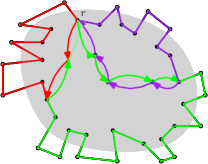
Figure 3: (a) A cluster and a cycle whose cost inside the cluster is much larger than the scale. The numbers indicate the counter values on the cost of the cycle at that vertex. (b) Two paths added to each special vertex, the directions are only for emphasis. (c) A decomposition into three cycles.

4.2.2 Properties

Lemma 4.8.

In a call to Patch$(C,c,\Delta_{\ell})$, each cycle formed by patching $C$ consists of edges in $C$ and edges internal to $K(c)$.

Proof.

Each edge in such a cycle that is not in the original cycle $C$ is in one of the shortest paths in the graph induced by $K(y)$. ∎

Corollary 4.9.

For any partition node $p$ that is not a descendant of $c$, if $C$ is $Z$-amenable for $p$ then so is every cycle obtained by patching it.

Proof.

By $Z$-amenability, at most $Z$ edges of $C$ cross $\pi(p)$. Let $C^{\prime}$ be a cycle formed by patching $C$. By Lemma 4.8, an edge in $C^{\prime}-C$ is internal to $K(c)$, so it cannot cross $\pi(p)$. Thus at most $Z$ edges of $C^{\prime}$ cross $\pi(p)$. ∎

Claim 4.10.

Consider the call Patch$(C,c,\Delta_{\ell})$. The cost of the shortest path from $r$ to each special vertex is at most $\Delta_{\ell}$.

Proof.

Let $p$ be the parent of $c$. Assume $p$ is not the root, and let $c^{\prime}$ be the parent of $p$. Because $C$ is valid for $c$ (a precondition for the call), for every proper ancestor of $c$ that is a cluster node, and in particular for the grandparent $c^{\prime}$ of $c$, and for some ancestor $C^{\prime}$ of $C$. $\psi[c^{\prime},C^{\prime}]$ is an ancestor of $c$. Because $\psi[c^{\prime},C^{\prime}]$ is a child of $c^{\prime}$ and an ancestor of $c$, it must be the parent $p$ of $c$. Therefore, in some execution of line (3), $p=p_{i,\kappa}$ where

• $\pi_{i}$ is a $\Delta_{\ell}$-bounded partition of $K(c^{\prime})$,

• $\kappa$ is the set of parts of $\pi$ that intersect $C$,

• $\pi_{i,\kappa}=\textsc{MergeParts}(\pi_{i},\kappa)$, and

• $\pi(p_{i,\kappa})=\pi_{i.\kappa}$.

If $C$ has no vertices in $K(c)$ then $\operatorname{cost}(C\cap G^{*}[K(c)])$ is zero so Patch$(C,c,\delta_{\ell})$ does not change $C$. Suppose $C$ has some vertex $v$ in $K(c)$. Because $c$ is a child of $p$, $K(c)$ is a part of $\pi(p_{i,\kappa})=\pi_{i,\kappa}$. Each part of $\pi_{i,\kappa}$ is obtained by merging a part of $\pi_{i}$ belonging to $\kappa$ with some parts of $\pi_{i}$ not in $\kappa$. Let $S$ be the part of $\pi_{i}$ that contains $v$. Because $S$ is the only part belonging to $\kappa$ that is a subset of $K(c)$, every vertex in $C\cap K(c)$ belongs to $S$. In particular, all the vertices designated as special in Patch belong to $S$. Because $S$ is a part of $\pi_{i}$, it has diameter at most $\Delta_{\ell}$. This proves the claim. ∎

Corollary 4.11.

If cycle $C^{\prime}$ is one of the cycles produced by patching cycle $C$ then the sum of costs of non-special edges in $C^{\prime}\cap G^{*}[K(c)]$ is at most $(\frac{Z}{3}+2)\cdot\Delta_{\ell}$.

Corollary 4.12.

The total cost of edges that are in cycles formed by patching $C$ and are not in $C$, taking into account multiplicity, is at most

$$2\,\left(\frac{\operatorname{cost}(C\cap G^{*}[K(c)])}{(Z/3)\cdot\Delta_{\ell}}\right)2\Delta_{\ell}.$$

Proof.

The number of shortest paths added is twice the number of special vertices. For each special vertex other than the starting vertex, the algorithm scans a portion of $C\cap G^{*}[K(c)]$ of cost greater than $(Z/3)\cdot\Delta_{\ell}$. Let $\eta$ be the smallest cost scanned. The number of special vertices is at most

$$1+\left\lfloor\frac{\operatorname{cost}(C\cap G^{*}[K(c)])}{\eta}\right\rfloor$$

which is at most

$$\left\lceil\frac{\operatorname{cost}(C\cap G^{*}[K(c)])}{(Z/3)\cdot\Delta_{\ell}}\right\rceil.$$

which is at most $2\frac{\operatorname{cost}(C\cap G^{*}[K(c)])}{(Z/3)\cdot\Delta_{\ell}}$ because $\operatorname{cost}(C\cap G^{*}[K(c)])>(Z/3)\cdot\Delta_{\ell}$. ∎

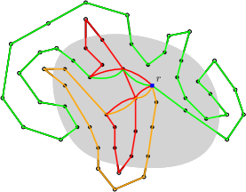
Figure 4: Another example of patching, with a more complicated cycle; this time the special vertices correspond to vertices where the counter is a multiple of $8$.

4.3 The remaining proofs

Now we restate and prove the remaining lemmas from §4.1.

See 4.2

Proof.

The patching procedure applied to a cycle $C$ ensures that each edge appears an odd number of times in the resulting cycles (counting multiplicity) iff the edge belongs to $C$. It follows from Lemma 2.4 that every two faces separated by $C$ are separated by at least one of the cycles resulting from patching. The lemma then follows by induction. ∎

See 4.3

Proof of Lemma 4.3.

Consider iteration $\ell$ of the virtual procedure, which operates on cluster nodes $c$ having level $\ell$. Let $\mathcal{C}_{\ell}$ denote the set $\mathcal{C}$ at the end of this iteration. For a cycle $C\in\mathcal{C}_{\ell}$, consider the cluster nodes at this level. The clusters $K(c)$ corresponding to these nodes are disjoint, and hence edges internal to these clusters are disjoint.

Now let $c$ be one such cluster node. For cycle $C\in\mathcal{C}_{\ell}$, define $\mathcal{C}(c,C)$ as the set of cycles $C^{\prime}$ that are ancestors of $C$ that were valid and patched at the time $c$ was processed by the virtual procedure $\mathcal{V}$. For each cycle $C^{\prime}\in\mathcal{C}(c,C)$, Corollary 4.12 bounds the increase in total cost due to patching $C^{\prime}$. Hence, the total increase during iteration $\ell$ is at most

$$\sum_{C\in\mathcal{C}_{\ell}}\quad\sum_{c\text{ at level }\ell}\quad\sum_{C^{\prime}\in\mathcal{C}(c,C)}2\,\left(\frac{\operatorname{cost}(C^{\prime}\cap G^{*}[K(c)])}{(Z/3)\cdot\Delta_{\ell}}\right)2\Delta_{\ell}$$

$$\leq\frac{12}{Z}\sum_{C\in\mathcal{C}_{\ell}}\operatorname{cost}(C)$$

where we use the fact that for each cycle $C\in\mathcal{C}_{\ell}$, the relevant valid clusters are disjoint.

We have shown that iteration $\ell$ increases the cost by at most a factor of $1+\nicefrac{{12}}{{Z}}$. Because the number of iterations is $O(\log n)$, we can choose $Z=O(\varepsilon^{-1}\log n)$ so that the total increase over all iterations is at most $1+\varepsilon$. ∎

See 4.6

Proof of Lemma 4.6.

Let $\bar{C}$ be a cycle in the final collection $\mathcal{C}$. The nodes of $\mathcal{T}$ for which $\bar{C}$ is valid form an ordinary hierarchical partition of $G^{*}$. Define $\varphi_{\bar{C}}$ as the function that maps each such cluster node $c$ to its unique partition node child $p$ in this ordinary hierarchical partition; validity implies that $\psi[c,C]=p$ for an ancestor $C$ of $\bar{C}$.

Let $p$ be a partition node of $\mathcal{T}|_{\varphi_{\bar{C}}}$. Let $c$ be the parent of $p$. By definition of validity, $\psi[c,C]$ was assigned $p$ for some ancestor $C$ of $\bar{C}$.

Case 1: $\psi[c,C]$ was assigned $p$ in some execution of Algorithm 3. In this case, $\pi(p)=\pi_{i,\kappa}$ where $i$ is selected in Algorithm 3 and $\kappa$ is selected in Algorithm 3 and $\pi_{i,\kappa}$ is derived in Algorithm 3 by application of MergeParts to $\pi_{i}$ and $\kappa$. By choice of $i$ in Algorithm 3, at most $Z$ edges of $C$ cross $\pi_{i}$, so the same holds for $\pi_{i,\kappa}$.

Case 2: $\psi[c,C]$ was assigned $p$ in some execution of Algorithm 3. In this case, $c$ is a part of a partition $\pi_{i,\kappa}$ selected in iteration $\ell=\log{\operatorname{diameter}}(G^{*})$, where $i$ is selected in Algorithm 3 and $\kappa$ is selected in Algorithm 3 and $\pi_{i,\kappa}$ is derived in Algorithm 3 by application of MergeParts to $\pi_{i}$ and $\kappa$. Because $\pi_{i}$ is a $\Delta_{\log{\operatorname{diameter}}(G^{*})+1}$-bounded partition, each part of $\pi_{i}$ has diameter less than one, but edge-lengths are integral and positive, so each part consists of a single vertex. By choice of $\kappa$ and definition of MergeParts, each part of $\pi_{i,\kappa}$ contains at most one part $P$ of $\pi_{i}$ that contains an endpoint of an edge of $C$ internal to $K(c)$, which implies that no edge of $C$ is internal to a part of $\pi_{i,\kappa}$. Therefore $C$ is 0-amenable for the shattering partition node of Algorithm 3. ∎

See 4.7

Proof of Lemma 4.7.

Consider iteration $\ell$ of the virtual procedure. Let $\mathcal{C}_{\ell}$ denote the set $\mathcal{C}$ at the end of this iteration. For a cycle $\bar{C}\in\mathcal{C}_{\ell}$, consider the cluster nodes at this level for which $C$ is valid. The clusters $K(c)$ corresponding to these nodes $c$ are disjoint, and hence there are at most $n$ such clusters.

For such a cluster node $c$, consider the ancestor $C$ of $\bar{C}$ such that $\psi[c,C]$ is assigned a partition node in Algorithm 3. Since $C$ was the result of patching a cycle with respect to $c$, Corollary 4.11 implies that the cost of non-special edges in $C$ is at most $(\nicefrac{{Z}}{{3}}+2)\Delta_{\ell}$. By the properties of random $\Delta$-bounded partitions, the expected number of nonspecial edges of $C$ crossing the random $\Delta_{\ell+1}$-bounded partition is bounded by $(Z/3+2)\cdot\frac{\Delta_{\ell}}{\Delta_{\ell+1}}$, which is $2(Z/3+2)$. Counting the single special edge in the cycle, the expected number of edges internally crossing the partition is at most $2Z/3+5$. Therefore, by Markov’s inequality, the number is at most $Z$ with some constant probability.

Thus over all $O(\log n)$ iterations of the for-loop in Algorithm 3, the probability that none of them selects a $\Delta_{\ell+1}$-bounded partition with at most $Z$ edges of $C$ internally crossing the partition is at most $\exp\{O(a\log n)\}=1/n^{O(a)}$. Now we can take a naive union bound over all the cluster nodes $c$ at this level for which $\bar{C}$ is valid (of which there are at most $n$, since they are disjoint), over all cycles $\bar{C}\in\mathcal{C}_{\ell}$, and over all levels $\ell$. These are only $O(n^{3}\log n)$ events (see Corollary 4.4), so choosing $a$ to be a sufficiently large constant ensures that the success probability of the virtual procedure is at least $1-1/n$, as claimed. ∎

5 Finding a Sparse Cut via LPs

The structure theorem (Theorem 4.1) from §4 gives us a $t$-nondeterministic hierarchical clustering $\mathcal{T}$ of the dual graph $G^{*}$ that is $(Z,\varepsilon)$-friendly with high probability. Given such a clustering $\mathcal{T}$, we need to find a good forcing and a good “low-complexity” solution with respect to it. The natural approach to try is dynamic programming, but no such approach is currently known for non-uniform sparsest cut; for example, the problem is NP-hard even for treewidth-$2$ graphs. Hence we solve a linear program and round it. Our linear program is directly inspired by the Sherali-Adams approach for bounded-treewidth graphs, augmented with ideas specific to the planar case. It encodes a series of choices giving us a forcing, and also choices about how a $(1+\varepsilon)$-approximate solution crosses the resulting clustering. Of course, these choices are fractional, so we need to round them, which is where we lose the factor of $2$.

5.1 Notation

As in the previous sections, we work on the planar dual $G^{*}=(V^{*},E^{*})$. Given a partition $\pi$ of a vertex set $U\subseteq V^{*}$, let $\partial(\pi)$ denote the boundary, i.e., the faces in $G^{*}$ whose vertices are all in $U$ but belong to more than one part of this partition; see Figure 5. Recall that for a partition node $p$ with parent cluster node $c$, we defined $\pi(p)$ as a partition of $K(c)$. In this section, we would like to extend the partition to all of $V^{*}$ by looking at the partition nodes that are ancestors of $p$. For a (cluster or partition) node $a$ in the tree, define $\textsf{partn\_path}(a)$ as the partition nodes on the path from the root of $\mathcal{T}$ to $a$, inclusive.

For a partition node $p$ with parent cluster node $c$, define $\pi^{+}(p)$ as the following partition of $V^{*}$: its parts are the parts of $\pi(p)$, together with all parts $P$ in $\pi(p^{\prime})$ over all partition nodes $p^{\prime}\in\textsf{partn\_path}(p)$, except the parts $P$ that contain $K(c)$. By the hierarchical nature of $\mathcal{T}$, these parts form a valid partition of $V^{*}$, which we call $\pi^{+}(p)$. For ease of notation, we abbreviate $\partial(p):=\partial(\pi(p))$ and $\partial^{+}(p):=\partial(\pi^{+}(p))$. While we will not need it, the reader can verify that $\partial^{+}(p)=\biguplus_{p^{\prime}\in\textsf{partn\_path}(p)}\partial(p^{\prime})$, where the $\biguplus$ indicates disjoint union.

For any simple cycle $C$ in $G^{*}$, let $\textsf{inside}(C)$ be the set of faces of $G^{*}$ (corresponding to vertices of $G$) inside $C$. Informally, we now define $\mathcal{A}^{+}(p)$ as the collection of all subsets of $\partial^{+}(p)$ that can comprise the faces of $\partial^{+}(p)$ inside any cycle $C$ in $G^{*}$ that is $Z$-amenable for each partition node $p^{\prime}\in\textsf{partn\_path}(p)$. Formally, $A^{+}(p)$ is the set

$$\mathcal{\{}\textsf{inside}(C)\cap\partial^{+}(p)\mid C\text{ is } \text{$Z$-amenable for all }p^{\prime}\in\textsf{partn\_path}(p)\}.$$

The following lemma lies at the heart of our “low-complexity” argument: the size of $\mathcal{A}^{+}(p)$ is quasi-polynomially bounded.

Lemma 5.1.

Let $\mathcal{T}$ be $(Z,\varepsilon)$-friendly with depth $H$. Then, $|\mathcal{A}^{+}(p)|\leq O(n)^{(H+1)Z}$, and we can compute it in time $O(n)^{O(H+1)Z}$.

Proof.

Consider a cycle $C$ that is $Z$-amenable for each normal partition node $p^{\prime}\in\textsf{partn\_path}(p)$ and $0$-amenable for each shattering partition node $p^{\prime}\in\textsf{partn\_path}(p)$. We first claim that $C$ must cross $\pi^{+}(p)$ at most $(H+1)Z$ times. Consider an edge $e$ in $C$ whose endpoints belong to different parts of $\pi^{+}(p)$. By construction of $\pi^{+}(p)$ and the $0$-amenability of $Z$ for shattering partition nodes, there must exist a normal partition node $p^{\prime}\in\textsf{partn\_path}(p)$ such that the endpoints of $e$ belong to different parts of $\pi(p^{\prime})$. In other words, we can charge each crossing of $\pi^{+}(p)$ to a crossing of some $\pi(p^{\prime})$ for some normal partition node $p^{\prime}\in\textsf{partn\_path}(p)$. Since $C$ is $Z$-amenable for normal partition node $p^{\prime}\in\textsf{partn\_path}(p)$, each one can be charged at most $Z$ times, and $|\textsf{partn\_path}(p)|\leq H+1$, so there are $(H+1)Z$ total crossings of $\pi^{+}(p)$.

Next, observe that if two cycles $C,C^{\prime}$ cross the same edges in $\pi^{+}(p)$, then $\textsf{inside}(C)\cap\partial^{+}(p)=\textsf{inside}(C^{\prime})\cap\partial^{+}(p)$, since they can only differ “within” parts of $\pi^{+}(p)$. It follows that $|\mathcal{A}^{+}(p)|$ is at most the number of ways to choose up to $(H+1)Z$ crossings of $\pi^{+}(p)$, which is $O(n)^{(H+1)Z}$.

We can compute $\mathcal{A}^{+}(p)$ as follows. First, guess the at most $Z$ crossings for each normal partition node $p^{\prime}\in\textsf{partn\_path}(p)$, and guess one of the at most $((H+1)Z)!$ cyclic orderings of the crossings. Not every cyclic ordering of crossings may correspond to a valid cycle, but it is easy to check in polynomial time whether a cycle exists, and if so, find such a cycle and subsequently compute $\textsf{inside}(C)\cap\partial^{+}(p)$. ∎

We now extend these definitions to pairs of nodes: for partition nodes $\{p,p^{\prime}\}$ in $\mathcal{T}$, define

• $\partial^{+}(\{p,p^{\prime}\}):=\partial^{+}(p)\cup\partial^{+}(p^{\prime})$, and

• $\mathcal{A}^{+}(\{p,p^{\prime}\}):=\{S_{p}\cup S_{{}^{\prime}p}\mid S_{p}\in\mathcal{A}^{+}(p),S_{p^{\prime}}\in\mathcal{A}^{+}(p^{\prime})\}$; note that $\mathcal{A}^{+}(\{p,p^{\prime}\})\supseteq\mathcal{A}^{+}(p)\cup\mathcal{A}^{+}(p^{\prime})$ and strict containment is possible.

Lemma 5.1 implies that $|\mathcal{A}^{+}(\{p,p^{\prime}\})|\leq n^{O(HZ)}$. Finally, for any two nodes $a$ and $b$ in $\mathcal{T}$, define $\textsf{lca}(a,b)$ as the lowest common ancestor node of $a$ and $b$ in $\mathcal{T}$.

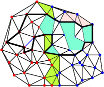
Figure 5: (a) A partition $\pi$ of vertices $U\subseteq V^{*}$ into three parts (with nodes in red, blue, and purple), and with the boundary $\partial(\pi)$ colored in. (b) A cycle $C$, and (c) the collection of faces $\textsf{inside}(C)\cap\partial(\pi)$ in bright blue. Since the cycle has $8$ edges cut, it is $Z$-amenable and this collection of faces belongs to $\mathcal{A}(\pi)$ as long as $Z\geq 8$.

5.2 Variables and Constraints

In this section, we introduce the variables and constraints of our linear program. If these variables were to take on Boolean values, they would encode a $Z$-amenable solution $C$. Of course, the optimal LP solution will be fractional, and we give the rounding in the next section. The consistency constraints will be precisely those needed for the rounding, and should be thought of as defining a suitable pseudo-distribution that can then be rounded.

Assume we start with a $Z$-friendly $\mathcal{T}$. We begin with defining the $x$-variables. For each partition node $p$ and set of (dual) faces $S\in\mathcal{A}^{+}(p)$, declare a variable $x(\{p\},S)$ with the constraint

$$0\leq x(\{p\},S)\leq 1,$$ (4)

which represents whether or not the sparsest cut solution $C$ (treated as a set of faces) satisfies $C\cap\partial^{+}(p)=S$. In other words, $x(\{p\},S)=1$ says that $S$ is the set of faces that lie inside the target solution, and also belong to $\partial(q)$ for some partition node $q$ that is either $p$ or an ancestor of $p$.

We also define variables that represent a “level-two lift” of these variables, which capture the same idea for pairs of faces. For each pair of distinct partition nodes $p,p^{\prime}$ whose lowest common ancestor $\textsf{lca}(p,p^{\prime})$ is a partition node, define a variable $x(\{p,p^{\prime\prime}\},S)$ with the constraint

$$0\leq x(\{p,p^{\prime\prime}\},S)\leq 1,$$ (5)

which represents whether or not $C\cap(\partial^{+}(\{p,p^{\prime\prime}\}))=S$.

Consistency. Next we impose “consistency” constraints on these variables. For the root node $\widehat{p}$, we add the constraint

$$x(\{\widehat{p}\},\varnothing)=1.$$ (6)

Recall that cluster partition nodes and cluster nodes alternate in $\mathcal{T}$, and recall the notion of forcing and relevance from Definition 3.4. We impose a constraint capturing (i) a “relaxation” of forcings and relevance, where each cluster node fractionally chooses one of its children partition nodes $p_{i}$, and (ii) a “relaxation” of determining which faces in $\partial^{+}(p_{i})$ (for the chosen $p_{i}$) are contained in $C$. Formally, for each cluster node $c$ whose parent is partition node $p$ and whose children are the partition nodes $p_{1},\ldots,p_{r}$, add the constraint

$$x(\{p\},S)=\sum_{\begin{subarray}{c}i\in[r],~{}S^{\prime}\in\mathcal{A}^{+}(p_{i}):\\ S^{\prime}\cap\partial^{+}(p)=S\end{subarray}}x(\{p_{i}\},S^{\prime}).$$ (7)

Projections. Next, we project the $x(\{p\},S)$ variables onto new auxiliary variables to capture whether the sparsest cut solution contains a dual face $s$, as well as to capture its intersection with $\mathcal{A}^{+}(p)$ on relevant partition nodes $p$. For a partition node $p$ and a face $s$, define $\mathcal{S}(p,s)$ as all partition nodes $p_{s}$ that (i) are either $p$ itself or descendants of $p$, and (ii) satisfy $s\in\partial(p_{s})$. (If $s$ is a face in $G^{*}[K(c)]$ where $c$ is the parent cluster node of $p$, then $s\in\partial(p_{s})$ for exactly one node along each path from $p$ to a leaf. On the other hand, if $s$ does not belong to $G^{*}[K(c)]$, then $\mathcal{S}(p,s)=\varnothing$, in which case the following definition is vacuous and the corresponding $z$ variable can be removed.)

For each face $s$, for each choice of $D$ being either $\varnothing$ or $\{s\}$, for each partition node $p$, and for each set of faces $W\in\mathcal{A}^{+}(p)$, define a variable $z(p,s,D,W)$ that captures whether (a) $p$ is relevant, (b) whether or not the sparsest cut solution $C$ contains face $s$ (depending on whether $D=\varnothing$ or $D=\{s\}$), and (c) whether $C$ has intersection $W$ with $\partial^{+}(p)$. We then add the constraint

$$z(p,s,D,W)=\sum_{\begin{subarray}{c}p_{s}\in\mathcal{S}(p,s),~{}S\in\mathcal{\partial}^{+}(p_{s}):\\ S\cap\{s\}=D\\ S\cap\partial^{+}(p)=W\end{subarray}}x(\{p_{s}\},S).$$

We do an analogous operation of projecting the $x(\{p_{1},p_{2}\},S)$ variables onto two faces, to capture costs and demands. For each partition node $p$ and for every two distinct faces $s,t$, consider all pairs of partition nodes $p_{s},p_{t}$ (not necessarily distinct) satisfying $s\in\partial(p_{s})$ and $t\in\partial(p_{t})$ and $\textsf{lca}(p_{s},p_{t})=p$. Let $\mathcal{S}(p,\{s,t\})$ be the collection of sets $\{p_{s},p_{t}\}$ over all such $p_{s},p_{t}$. (It is possible that $\mathcal{S}(p,\{s,t\})=\varnothing$, in which case again the following definition is vacuous and the corresponding variable can be removed.)

For each partition node $p$, for each subset $D\subseteq\{s,t\}$, for each set $\{p_{s},p_{t}\}\in\mathcal{S}(p,\{s,t\})$, and for each set $W\in\mathcal{A}^{+}(p)$, define a variable $y(p,\{s,t\},D,W)$ which captures whether (a) $p$ is relevant, (b) whether the sparsest cut solution $C$ has intersection $D$ with $\{s,t\}$ and (c) whether it has intersection $W$ with $\partial^{+}(p)$. Add the constraint

$$y(p,\{s,t\},D,W)=\sum_{\begin{subarray}{c}\{p_{s},p_{t}\}\in\mathcal{S}(p,\{s,t\}),~{}S\in\mathcal{A}^{+}(\{p_{s},p_{t}\}):\\ S\cap\{s,t\}=D\\ S\cap\partial^{+}(p)=W\end{subarray}}x(\{p_{s},p_{t}\},S).$$ (8)

We next enforce that the variables $z(\cdot)$ and $y(\cdot)$ must have “consistent marginals” when viewed as distributions. For each partition node $p$, for each subset $D\subseteq\{s\}$, and for each set $W\in\mathcal{A}^{+}(p)$, impose the constraint

$$z(p,s,D,W)=\sum_{\begin{subarray}{c}D^{\prime}\subseteq\{s,t\}:\\ D^{\prime}\cap\{s\}=D\end{subarray}}y(p,\{s,t\},D^{\prime},W).$$ (9)

Marginals. Finally, we define variables that do some further projection. We define a variable $y(\{s,t\})$ capturing the overall event that $s$ and $t$ are separated, and add the consistency constraint

$$y(\{s,t\})=\sum_{\begin{subarray}{c}\text{partition node }p,~{}D\subseteq\{s,t\}:\\ |D\cap\{s,t\}|=1,\\ W\in\mathcal{A}^{+}(p)\end{subarray}}y(p,\{s,t\},D,W).$$ (10)

Observe that combining (8) and (10) gives the equality

$$y(\{s,t\}) =\sum_{\begin{subarray}{c}\text{partition node }p,\\ D\subseteq\{s,t\}:\\ |D\cap\{s,t\}|=1,\\ W\in\mathcal{A}^{+}(p)\end{subarray}}y(p,\{s,t\},D,W)$$

$$=\sum_{\begin{subarray}{c}\text{partition node }p,\\ D\subseteq\{s,t\}:\\ |D\cap\{s,t\}|=1,\\ W\in\mathcal{A}^{+}(p)\end{subarray}}\sum_{\begin{subarray}{c}\{p_{s},p_{t}\}\in\mathcal{S}(p,\{s,t\}),\\ S\in\mathcal{A}^{+}(\{p_{s},p_{t}\}):\\ S\cap\{s,t\}=D\\ S\cap\partial^{+}(p)=W\end{subarray}}x(\{p_{s},p_{t}\},S)$$

$$=\sum_{\begin{subarray}{c}\text{partition node }p,\\ \{p_{s},p_{t}\}\in\mathcal{S}(p,\{s,t\}),\\ S\in\mathcal{A}^{+}(\{p_{s},p_{t}\}):\\ |S\cap\{s,t\}|=1\end{subarray}}x(\{p_{s},p_{t}\},S).$$ (11)

Consistency II. Finally, for the lifted variables $x(\{p_{s},p_{t}\},S)$, we define an additional consistency constraint that relates the original variables of (4) to the lifted variables of (5). For each partition node $p$ and set $W\in\mathcal{A}^{+}(p)$ and every pair $\{s,t\}$ of faces, add the constraint

$$x(\{p\},W)=\sum_{\begin{subarray}{c}\{p_{s},p_{t}\}\in\mathcal{S}(p,\{s,t\}):\\ S\in\mathcal{A}^{+}(\{p_{s},p_{t}\})\\ S\cap\partial^{+}(p)=W\end{subarray}}x(\{p_{s},p_{t}\},S).$$ (12)

The Cut Demand, and the Objective. We assume that we have an estimate $\alpha$ for the cut demand, which allows us to impose the constraint:

$$\sum_{s\neq t}y(\{s,t\})\geq\alpha.$$ (13)

Since the edges in the primal corresponding to pairs of faces in the dual that share a dual edge, the objective function is:

$$\text{minimize }\sum_{\{s,t\}:s\cap t\in E^{*}}\operatorname{cost}(\{s,t\})y(\{s,t\}),$$

This completes the definition of the linear program for the guess $\alpha$.

Lemma 5.2.

For $\varepsilon\leq 1$, let $\mathcal{T}$ be a $(Z,\varepsilon)$-friendly nondeterministic hierarchical decomposition. We can write $O(\varepsilon^{-1}\log n)$ LPs of the form above, such that one of them has a feasible solution with fractional cost at most $(1+O(\varepsilon))\alpha\,\Phi^{*}$.

Proof.

We write an LP for each setting of $\alpha$ being a power of $(1+\varepsilon)$, lying between $1$ and $n^{5}$, which is an upper bound on the separated demand by Lemma 2.1. By the definition of $\mathcal{T}$ being $(Z,\varepsilon)$-friendly, there exists a forcing $\varphi$ of the cluster nodes of $\mathcal{T}$ and a sparsest cut solution $C$ that has sparsity at most $(1+\varepsilon)$ times the optimal sparsity, and is $Z$-amenable for the forced tree $\mathcal{T}|_{\varphi}$. Focus on the linear program for $\alpha$ being the largest power of $(1+\varepsilon)$ which is no larger than the demand separated by $C$. Setting the variables above according to this solution $C$ and the forcing $\varphi$ gives a $0$-$1$ solution each of the linear programs. Now the cost of the cycle $C$ is the sparsity of $C$ times the demand separated, i.e., at most $(1+\varepsilon)\Phi^{*}\cdot(1+\varepsilon)\alpha$ as claimed. ∎

5.3 Rounding the LP

We round the LP solution top-down, beginning with the root partition node. Our goal is to select a forcing of cluster nodes to their child partition nodes, as well as select an element of $\mathcal{A}(p)$ for each partition node $p$ that we round, which turns out to be all relevant face nodes under the chosen forcing. Our final solution will be a set $U$ of faces. Initially, $U=\varnothing$; we will add to $U$ at each partition node that we round.

• For a cluster node $c$ with parent node $p$ and children $p_{1},\ldots,p_{r}$, we have already rounded $\mathcal{A}^{+}(p)$ by this point; that is, we have already determined $U\cap\partial(p)$, which we call $W$. We assign partition node $p_{i}$ to cluster node $c$ with probability

  $$\frac{1}{x(\{p\},W)}\sum_{\begin{subarray}{c}S\in\mathcal{A}^{+}(p_{i}):\\ S\cap\partial^{+}(p)=W\end{subarray}}x(\{p_{i}\},S).$$

  This is a probability distribution by (7).

• For the chosen partition node $p_{i}$, we need to determine which faces in $\partial(p_{i})$ are in $U$. We want to choose a set $S\in\mathcal{A}^{+}(p_{i})$ satisfying $S\cap\partial^{+}(p)=W$, and then add $S\setminus W$ to $U$. We simply choose one with probability proportional to $x(\{p_{i}\},S)$. That is, each set $S\in\mathcal{A}^{+}(p_{i})$ satisfying $S\cap\partial^{+}(p)=W$ is chosen with probability

  $$x(\{p_{i}\},S)\cdot\bigg{(}\sum_{\begin{subarray}{c}S^{\prime}\in\mathcal{A}^{+}(p_{i}):\\ S^{\prime}\cap\partial^{+}(p)=W\end{subarray}}x(\{p_{i}\},S^{\prime})\bigg{)}^{-1},$$

  which is clearly a probability distribution. We then add $S\setminus W$ to $U$.

We begin with a lemma similar to [GTW13, Lemma 2.2]:

Lemma 5.3.

For any partition node $p$ and set $S\in\mathcal{A}^{+}(p)$, the probability that $p$ is relevant and $U\cap\partial^{+}(p)=S$ is $x(\{p\},S)$.

Proof.

We show this by induction from the root down the tree. Let $p^{\prime}$ be a partition node, let $c$ be a child of $p^{\prime}$, and let $p$ be a child of $c$. By induction, for any set $W\in\mathcal{A}^{+}(p^{\prime})$, the probability that $p^{\prime}$ is relevant and $U\cap\partial^{+}(p^{\prime})=W$ is $x(\{p^{\prime}\},W)$.

Fix a set $S\in\mathcal{A}^{+}(p)$, define $W:=S\cap\partial^{+}(p)$, and condition on the event that $U\cap\partial^{+}(p^{\prime})=W$, which happens with probability $x(\{p^{\prime}\},W)$. Conditioned on this, partition node $p$ is relevant to cluster node $c$ with probability

$$\frac{1}{x(\{p^{\prime}\},W)}\sum_{S^{\prime}}x(\{p\},S^{\prime}),$$

where the summation is over all $S^{\prime}\in\mathcal{A}^{+}(p)$ satisfying $S^{\prime}\cap\partial^{+}(p^{\prime})=W$. Conditioned on this as well, set $S\in\mathcal{A}^{+}(p)$ is chosen with probability

$$\frac{x(\{p\},S)}{\sum_{S^{\prime}}x(\{p\},S^{\prime})},$$

with the same summation over $S^{\prime}$. Unraveling the conditioning, the overall probability of choosing $S\in\mathcal{A}^{+}(p)$ is

$$x(\{p^{\prime}\},W)\cdot\frac{1}{x(\{p^{\prime}\},W)}\sum_{S^{\prime}}x(\{p\},S^{\prime})\cdot\frac{x(\{p\},S)}{\sum_{S^{\prime}}x(\{p\},S^{\prime})}=x(\{p\},S),$$

as desired. ∎

Corollary 5.4.

For any edge $\{s,t\}$ of the primal graph $G$, the probability that $|U\cap\{s,t\}|=1$ is exactly $y(\{s.t\})$. Therefore, the expected total cost of the primal edges cut is equal to the fractional value of the LP.

Proof.

Consider the partition node $p$ that separates $s$ and $t$; such a node exists because all leaf cluster nodes are singletons. Since $\{s,t\}$ is an edge of the primal graph, one or both of the dual faces $s$ and $t$ is in $\partial(p)$. Assume without loss of generality that $s\in\partial(p)$. Consider the partition node $p_{t}$ with $t\in\partial(p_{t})$. Since $p_{t}$ is a descendant of $p$, we have $\mathcal{A}^{+}(\{p,p_{t}\})=\mathcal{A}^{+}(p_{t})$, and moreover, both $s$ and $t$ are in $\mathcal{A}^{+}(p_{t})$. For any $S\in\mathcal{A}^{+}(p_{t})$ such that $|S\cap\{s,t\}|=1$, by Lemma 5.3, the probability that $p$ is relevant and $U\cap\partial^{+}(p_{t})=S$ is $x(\{p_{t}\},S)$. These probability events are all disjoint, so the total probability that $|U\cap\{s,t\}|=1$ is

$$\sum_{\begin{subarray}{c}p\text{ separates $s,t$},\\ S\in\mathcal{A}^{+}(\{p,p_{t}\}):\\ |S\cap\{s,t\}|=1\end{subarray}}x(\{p,p_{t}\},S)\stackrel{{\scriptstyle(\ref{eq:yst2})}}{{=}}y(\{s,t\}).$$

The expected total cost follows by linearity of expectation. ∎

Lemma 5.5.

For each $\{s,t\}\in E^{*}$, we have $\Pr[|U\cap\{s,t\}|=1]=y(\{s,t\})$, and for each $\{s,t\}\in\mathcal{D}$, we have $\Pr[|U\cap\{s,t\}|=1]\geq\frac{1}{2}\,y(\{s,t\})$.

Proof.

Let $p_{s}$ be the unique relevant partition node satisfying $s\in\partial(p_{s})$, and let $p_{t}$ be the unique relevant partition node satisfying $t\in\partial(p_{t})$. Let $p$ be the lowest common ancestor of $p_{s}$ and $p_{t}$, which must be a relevant partition node. Under the randomness of selecting the forcing in the LP rounding, $p_{s},p_{t},p$ are random variables. Define $W:=U\cap\partial(S)$, which is also a random variable. We claim that

$$\mathbb{E}_{p,W}\bigg{[}\frac{1}{x(\{p\},W)}\sum_{\begin{subarray}{c}\{p_{s},p_{t}\}\in\mathcal{S}(p,\{s,t\}):\\ S\in\mathcal{A}^{+}(\{p_{s},p_{t}\}):\\ S\cap\partial^{+}(p)=W\\ |S\cap\{s,t\}|=1\end{subarray}}x(\{p_{s},p_{t}\},S)\bigg{]}=y(\{s,t\}).$$ (14)

This is because the probability of choosing a particular $p,W$ is $x(\{p\},W)$ by Lemma 5.3, and

$$\mathbb{E}_{p,W} \bigg{[}\frac{1}{x(\{p\},W)}\sum_{\begin{subarray}{c}\{p_{s},p_{t}\}\in\mathcal{S}(p,\{s,t\}):\\ S\in\mathcal{A}^{+}(\{p_{s},p_{t}\}):\\ S\cap\partial^{+}(p)=W\\ |S\cap\{s,t\}|=1\end{subarray}}x(\{p_{s},p_{t}\},S)\bigg{]}$$

$$=\sum_{p,W}x(\{p\},W)\cdot\bigg{[}\frac{1}{x(\{p\},W)}\sum_{\begin{subarray}{c}\{p_{s},p_{t}\}\in\mathcal{S}(p,\{s,t\}):\\ S\in\mathcal{A}^{+}(\{p_{s},p_{t}\}):\\ S\cap\partial^{+}(p)=W\\ |S\cap\{s,t\}|=1\end{subarray}}x(\{p_{s},p_{t}\},S)\bigg{]}$$

$$=\sum_{p,W}\sum_{\begin{subarray}{c}\{p_{s},p_{t}\}\in\mathcal{S}(p,\{s,t\}):\\ S\in\mathcal{A}^{+}(\{p_{s},p_{t}\}):\\ S\cap\partial^{+}(p)=W\\ |S\cap\{s,t\}|=1\end{subarray}}x(\{p_{s},p_{t}\},S)$$

$$=\sum_{\begin{subarray}{c}\text{partition node }p,\\ \{p_{s},p_{t}\}\in\mathcal{S}(p,\{s,t\})\end{subarray}}\sum_{\begin{subarray}{c}S\in\mathcal{A}^{+}(\{p_{s},p_{t}\}):\\ |S\cap\{s,t\}|=1\end{subarray}}x(\{p_{s},p_{t}\},S)$$

$$\stackrel{{\scriptstyle(\ref{eq:yst2})}}{{=}}y(\{s,t\}).$$

First, suppose that $\{s,t\}\in E^{*}$. Then, we must have either $p_{s}=p$ or $p_{t}=p$, since the first partition node “splitting” off $s$ and $t$ must contain either $s$ or $t$. Let $p^{\prime}\in\{p_{s},p_{t}\}$ be the node that is not $p$. Then, by Lemma 5.3, for any $p^{\prime}$ and $S\in\mathcal{A}^{+}(p^{\prime})$, the probability that $p^{\prime}$ is relevant and $U\cap\partial^{+}(p)=S$ is $x(\{p^{\prime}\},S)$. Conditioned on the choices of random variables $p$ and $W$, for any $p^{\prime}$ that is a descendant of $p$, the probability that $p^{\prime}$ is relevant and $U\cap\partial^{+}(p)=S$ is $\frac{x(\{p^{\prime}\},S)}{x(\{p\},W)}$. Using that $x(\{p^{\prime}\},S)=x(\{p,p^{\prime\prime}\},S)$ since $p^{\prime}$ is a descendant of $p$, this probability is also $\frac{x(\{p,p^{\prime\prime}\},S)}{x(\{p\},W)}$. Also, since $p^{\prime}$ is a descendant of $p$, we have $\mathcal{A}^{+}(p^{\prime})=\mathcal{A}^{+}(\{p,p^{\prime\prime}\})$. Therefore, conditioned on the choices of $p$ and $W$, the probability that $U$ separates $s$ and $t$ is

$$\sum_{\begin{subarray}{c}p^{\prime}\text{ descendant of }p,\\ S\in\mathcal{A}^{+}(p^{\prime}):\\ |S\cap\{s,t\}|=1\end{subarray}}\frac{x(\{p,p^{\prime\prime}\},S)}{x(\{p\},W)}=\sum_{\begin{subarray}{c}\{p_{s},p_{t}\}\in\mathcal{S}(p,\{s,t\}),\\ S\in\mathcal{A}^{+}(\{p_{s},p_{t}\}):\\ S\cap\partial^{+}(p)=W\\ |S\cap\{s,t\}|=1\end{subarray}}\frac{x(\{p_{s},p_{t}\},S)}{x(\{p\},W)},$$

which is exactly the term inside the expectation in (14). Unraveling the conditioning on the choices of $p$ and $W$ and using (14), the probability that $U$ separates $s$ and $t$ is $y(\{s,t\})$, as desired.

Now consider a pair $\{s,t\}\in\mathcal{D}$. Fix partition nodes $p_{s}\in\mathcal{S}(p,s)$ with $s\in\partial(s)$ and $t\in\partial(t)$. Conditioned on the choices of $p$ and $W\in\mathcal{A}^{+}(p)$, for each $p_{s}\in\mathcal{S}(p,s)$ and $S\in\mathcal{A}^{+}(p_{s})$ satisfying $S\cap\partial^{+}(p)=W$, the probability that both $p_{s}$ is relevant and $U\cap\mathcal{A}^{+}(p_{s})=S$ is $\frac{x(\{p_{s}\},S)}{x(\{p\},W)}$ by Lemma 5.3. Let $Z_{s}$ denote the random variable $U\cap\{s\}$; then, for each $D_{s}\subseteq\{s\}$,$\Pr[Z_{s}=D_{s}\mid p,W]$

$$=\frac{1}{x(\{p\},W)}\sum_{\begin{subarray}{c}p_{s}\in\mathcal{S}(p,s),\\ S\in\mathcal{A}^{+}(p_{s}):\\ S\cap\partial^{+}(p)=W\\ S\cap\{s\}=D_{s}\end{subarray}}x(\{p_{s}\},S)=\frac{z(p,s,D_{s},W)}{x(\{p\},W)}.$$

Similarly, conditioned on the choices of $p$ and $W$, for each $p_{t}\in\mathcal{S}(p,t)$ and $T\in\mathcal{A}^{+}(p_{t})$ satisfying $T\cap\partial^{+}(p)=W$, the probability that both $p_{t}$ is relevant and $U\cap\mathcal{A}^{+}(p_{t})=T$ is $\frac{x(\{p_{t}\},T)}{x(\{p\},W)}$. Let $Z_{t}$ denote the random variable $U\cap\{t\}$; then, for each $D_{t}\subseteq\{t\}$,$\Pr[Z_{t}=D_{t}\mid p,W]$

$$=\frac{1}{x(\{p\},W)}\sum_{\begin{subarray}{c}p_{t}\in\mathcal{S}(p,t),\\ T\in\mathcal{A}^{+}(p_{t}):\\ T\cap\partial^{+}(p)=W\\ T\cap\{t\}=D_{t}\end{subarray}}x(\{p_{t}\},T)=\frac{z(p,t,D_{t},W)}{x(\{p\},W)}.$$

Observe that for a given $\{p_{s},p_{t}\}\in\,S(p,\{s,t\})$ and $S\in\mathcal{A}^{+}(p_{s})$ and $T\in\mathcal{A}^{+}(p_{t})$ satisfying $S\cap\partial^{+}(p)=T\cap\partial^{+}(p)=W$, the sets $S\setminus W$ and $T\setminus W$ are disjoint. By the nature of the LP rounding algorithm, we have that conditioned on the choices of $p$ and $W$, the random variables $Z_{s}$ and $Z_{t}$ are independent.

Next, conditioned on the choices of $p$ and $W$, let $Y$ be a random variable that takes each value $D\subseteq\{s,t\}$ with probability $\frac{y(p,\{s,t\},D,W)}{x(\{p\},W)}$. This is a probability distribution because

$$\sum_{D\subseteq\{s,t\}}\Pr[Y=D\mid p,W]=\sum_{D\subseteq\{s,t\}}\frac{y(p,\{s,t\},D,W)}{x(\{p\},W)}$$

$$=\sum_{D\subseteq\{s,t\}}\frac{1}{x(\{p\},W)}\sum_{\begin{subarray}{c}\{p_{s},p_{t}\}\in\mathcal{S}(p,\{s,t\}),\\ S\in\mathcal{A}^{+}(\{p_{s},p_{t}\}):\\ S\cap\{s,t\}=D\\ S\cap\partial^{+}(p)=W\end{subarray}}x(\{p_{s},p_{t}\},S)$$

$$=\frac{1}{x(\{p\},W)}\sum_{\begin{subarray}{c}\{p_{s},p_{t}\}\in\mathcal{S}(p,\{s,t\}),\\ S\in\mathcal{A}^{+}(\{p_{s},p_{t}\}):\\ S\cap\partial^{+}(p)=W\end{subarray}}x(\{p_{s},p_{t}\},S)$$

$$\stackrel{{\scriptstyle(\ref{eq:xfW})}}{{=}}1.$$

We now claim that $Y$, now viewed as a distribution on $\{\varnothing,\{s\}\}\times\{\varnothing,\{t\}\}$ (instead of on the power set of $\{s,t\}$), agrees with $Z_{s}(\cdot)$ and $Z_{t}(\cdot)$ on the marginals. Namely, for $D_{s}\subseteq\{s\}$, we have

$$\sum_{\begin{subarray}{c}D\subseteq\{s,t\}:\\ D\cap\{s\}=D_{s}\end{subarray}}\Pr[Y=D\mid p,W] =\sum_{\begin{subarray}{c}D\subseteq\{s,t\}:\\ D\cap\{s\}=D_{s}\end{subarray}}\frac{y(p,\{s,t\},D,W)}{x(\{p\},W)}$$

$$\stackrel{{\scriptstyle(\ref{eq:marginals})}}{{=}}\frac{z(p,s,D,W)}{x(\{p\},W)}$$

$$=\Pr[Z_{s}=D_{s}\mid p,W],$$ (15)

and for $D_{t}\subseteq\{t\}$, we similarly have

$$\sum_{\begin{subarray}{c}D\subseteq\{s,t\}:\\ D\cap\{t\}=D_{s}\end{subarray}}\Pr[Y=D\mid p,W]=\Pr[Z_{t}=D_{t}\mid p,W].$$ (16)

Claim 5.6.

Define event $\mathcal{E}$ to be $((Z_{s}=\{s\})\wedge(Z_{t}=\varnothing))\vee((Z_{s}=\varnothing)\wedge(Z_{t}=\{t\}))$. Then

$$\Pr[\;\mathcal{E}\mid p,W]\geq\frac{1}{2}\,\Pr[(Y=\{s\})\vee(Y=\{t\})\mid p,W],$$ (17)

Assuming Claim 5.6, the probability that solution $U$ separates $s$ and $t$ conditioned on $p$ and $W$ is

$$\Pr[ |U\cap\{s,t\}|=1\mid p,W]$$

$$=\Pr[\;\mathcal{E}\mid p,W]$$

$$\geq\frac{1}{2}\,\Pr[(Y=\{s\})\vee(Y=\{t\})\mid p,W]$$

$$=\frac{1}{2}\,\left(\frac{y(p,\{s,t\},\{s\},W)}{x(\{p\},W)}+\frac{y(p,\{s,t\},\{t\},W)}{x(\{p\},W)}\right)$$

$$=\frac{1}{2}\,\bigg{(}\frac{1}{x(\{p\},W)}\sum_{\begin{subarray}{c}\{p_{s},p_{t}\}\in\mathcal{S}(p,\{s,t\}),\\ S\in\mathcal{A}^{+}(\{p_{s},p_{t}\}):\\ S\cap\partial^{+}(p)=W\\ |S\cap\{s,t\}|=1\end{subarray}}x(\{p_{s},p_{t}\},S),\bigg{)}$$

which is half of the term inside the expectation in (14). Finally, unraveling the conditioning on the choices of $p$ and $W$ and using (14), we obtain

$$\Pr[|U\cap\{s,t\}|=1]\geq\frac{1}{2}\,y(\{s,t\}),$$

which concludes Lemma 5.5. ∎

Corollary 5.7.

Let cost be the total cost of the primal edges cut, and let demand be the total demands cut. Let $\Phi^{*}$ be the optimal sparsity. Then, $\mathbb{E}[\mathsf{cost}-2(1+O(\varepsilon))\cdot\Phi^{*}\cdot\mathsf{demand}]\leq 0$.

Proof.

By Theorem 4.1, there is a $t$-nondeterministic $(Z,\varepsilon)$-friendly hierarchical decomposition $\mathcal{T}$. Given $\mathcal{T}$, Lemma 5.2 says that there is a feasible solution to the LP with fractional demand at least $\alpha$ and fractional cost at most $(1+O(\varepsilon))\alpha\Phi^{*}$. By Corollary 5.4, $\mathbb{E}[\mathsf{cost}]$ equals the fractional cost of the LP, which is at most $(1+O(\varepsilon))\alpha\Phi^{*}$, and by Lemma 5.5, $\mathbb{E}[\mathsf{demand}]\geq\frac{1}{2}\,\alpha$, so we are done. ∎

This implies that $\mathbb{E}[\mathsf{cost}]/\mathbb{E}[\mathsf{demand}]\leq 2(1+O(\varepsilon))\cdot\Phi^{*}$. While this ratio of expectations is normally not enough, we can use Lemma A.2 to find a cut of sparsity at most $2(1+O(\varepsilon))\Phi^{*}$ with high probability, and hence complete the algorithm. It just remains to prove Claim 5.6.

Proof of Claim 5.6.

Define

$$a :=\Pr[Y=\{\varnothing\}\mid p,W] \qquad b :=\Pr[Y=\{s\}\mid p,W]$$ (18)

$$c :=\Pr[Y=\{t\}\mid p,W] d :=\Pr[Y=\{s,t\}\mid p,W],$$ (19)

so that $a+b+c+d=1$. By (15) and (16),

$$\Pr[Z_{s}=\varnothing\mid p,W]=\sum_{\begin{subarray}{c}D\subseteq\{s,t\}:\\ D\cap\{s\}=\varnothing\end{subarray}}\Pr[Y=D\mid p,W]=a+c,$$

$$\Pr[Z_{s}=\{s\}\mid p,W]=\sum_{\begin{subarray}{c}D\subseteq\{s,t\}:\\ D\cap\{s\}=\{s\}\end{subarray}}\Pr[Y=D\mid p,W]=b+d,$$

$$\Pr[Z_{t}=\varnothing\mid p,W]=\sum_{\begin{subarray}{c}D\subseteq\{s,t\}:\\ D\cap\{t\}=\varnothing\end{subarray}}\Pr[Y=D\mid p,W]=a+b,$$

$$\Pr[Z_{t}=\{t\}\mid p,W]=\sum_{\begin{subarray}{c}D\subseteq\{s,t\}:\\ D\cap\{t\}=\{t\}\end{subarray}}\Pr[Y=D\mid p,W]=c+d.$$

Since $Z_{s}$ and $Z_{t}$ are independent conditioned on the choices of $p$ and $W$,

$$\Pr[((Z_{s}=\{s\})\wedge(Z_{t}=\varnothing))\vee((Z_{s}=\varnothing)\wedge(Z_{t}=\{t\}))\mid p,W]$$

$$={} \Pr[Z_{s}=\{s\}\mid p,W]\cdot\Pr[Z_{t}=\varnothing\mid p,W]$$

$$~{}~{}~{}~{}~{}~{}~{}~{}~{}+\Pr[Z_{s}=\varnothing\mid p,W]\cdot\Pr[Z_{t}=\{t\}\mid p,W]$$

$$={} (b+d)(a+b)+(a+c)(c+d)$$

Moreover,

$$\Pr[(Y=\{s\})\vee(Y=\{t\})\mid p,W]=b+c,$$

so (17) now follows from Proposition A.1. This concludes the proof of Lemma 5.5. ∎

6 Concluding Remarks

A natural question is whether there is a polynomial-time $2+\epsilon$ approximation algorithm. Another is whether a 2-approximation or even better can be achieved in quasi-polynomial time. Note that no approximation ratio smaller than two is known even for the special case of series-parallel graphs (which are planar and have treewidth two). The greatest approximation lower bound known (assuming the unique games conjecture) is $\approx(1.139-\varepsilon)$, via a relatively simple reduction is from Max-Cut [GTW13]. Given the known limitations of linear programming techniques for Max-Cut, we may need to use semidefinite programs to obtain an approximation ratio better than two. Another question is whether the result can be extended to more general families of graphs such as minor-free graphs.

Appendix A Missing Proofs

A.1 The Decoupling Lemma

Proposition A.1.

Given non-negative numbers $a,b,c,d$ with sum $a+b+c+d=1$,

$$L:=(a+b)(b+d)+(a+c)(c+d)\geq\nicefrac{{1}}{{2}}\cdot(b+c)$$ (20)

Proof.

We have

$$1=(a+b+c+d)^{2} =a^{2}+b^{2}+c^{2}+d^{2}+2(ab+ac+ad+bc+bd+cd)$$

$$=2(ab+ac+2ad+b^{2}+bd+c^{2}+cd)+a^{2}+d^{2}-2ad-b^{2}-c^{2}+2bc$$

$$=2L+(a-d)^{2}-(b-c)^{2},$$

which gives now gives the claimed bound:

$$b+c=1-(a+d)=\big{(}2L+(a-d)^{2}-(b-c)^{2}\big{)}-(a+d)\leq 2L.$$

The inequality above uses that $(b-c)^{2}\geq 0$ and $(a-d)^{2}\leq a+d$ for $a,d\in[0,1]$. To see the latter, let $a\leq d$ without loss of generality and let $\varepsilon=d-a$. Since $\varepsilon\in[0,1]$ it follows that $\varepsilon^{2}\leq\varepsilon\leq 2a+\varepsilon$. ∎

A.2 The Expectation Lemma

Lemma A.2.

Given a randomized algorithm $A$ for sparsest cut which outputs a cut $(U,V\setminus U)$ that has $\mathbb{E}[\operatorname{cost}(U)]/\mathbb{E}[\operatorname{demand}(U)]\leq\alpha$ for some polynomially-bounded $\alpha$, there is a procedure that outputs a cut with $\operatorname{cost}(U)/\operatorname{demand}(U)\leq(1+o(1))\alpha$ in polynomial time, with probability $1-\nicefrac{{1}}{{n}}$.

Proof.

There are several ways to perform this conversion: e.g., we can the approach of [CKR10, GTW13] of derandomizing the algorithm to find the desired cut. But here is a different and conceptually simpler approach. Firstly, by running $A$ independently several times until it returns a cut with finite sparsity, we can assume that $A$ always returns a cut that separates some demands. (This is just conditioning on the event that $A$ outputs a finite-sparsity cut.) Because all edge costs and demands are polynomially bounded by Lemma 2.1, we need to repeat $A$ at most polynomially many times for this to happen. Also, the ratio of the expected cost to the expected demand does not increase by this conditioning.

Run the algorithm independently $N$ times to get cuts $U_{1},\ldots,U_{N}$, and return the sparsest cut among the ones returned. By Lemma 2.1 both the costs and demands of the cuts are bounded between $1$ and $n^{5}$; hence if $N=n^{c}$ for suitably large constant $c$, a Chernoff bound implies that the average cost and demand among these $N$ samples are both within a $(1\pm\nicefrac{{1}}{{n}})$ factor of their expectations with high probability, and hence

$$\frac{\sum_{i}\operatorname{cost}(U_{i})}{\sum_{i}\operatorname{demand}(U_{i})}\leq\frac{\alpha(1+\nicefrac{{1}}{{n}})}{(1-\nicefrac{{1}}{{n}})}.$$

Now using that $\min_{i}\operatorname{cost}(U_{i})/\operatorname{demand}(U_{i})\leq\frac{\sum_{i}\operatorname{cost}(U_{i})}{\sum_{i}\operatorname{demand}(U_{i})}$ completes the argument. ∎

A.3 Proofs from Section 2

Proof of Lemma 2.1.

Let $G$ be an instance of sparsest cut on a planar graph with $n$ verticeas. We guess the edge $e_{\max}$ with largest cost that is part of the sparsest cut $U^{*}$ in $G$, and contract all edges with cost larger than that of $e_{\max}$ (keeping parallel edges, and summing up the demand at the merged vertices). Moreover we round up the cost of each remaining edge to the closest multiple of $\operatorname{cost}(e_{\max})/n^{2}$ greater than it. Let $G^{\prime}$ be the resulting instance. Since no edge of the sparsest cut $U^{*}$ has been contracted during the procedure, it remains is a feasible solution for $G^{\prime}$, separating the same demand as in $G$. Moreover, its cost in $G^{\prime}$ is at most the cost of $U^{*}$ in $G$, plus the increase due to rounding up the edge costs. There are at most $O(n)$ such edges by planarity, so the total cost increase is at most $\operatorname{cost}(e_{\max})/n$.

It follows that the sparsity of each cut in $G^{\prime}$ is only higher than the corresponding cut in $G$, and moreover, there exists a cut in $G^{\prime}$ of sparsity at most $(1+\nicefrac{{1}}{{n}})$ times the optimal sparsity in $G$. Therefore, applying $\mathcal{A}$ on $G^{\prime}$ yields a solution for $G$ of sparsity at most $\alpha(1+o(1))$ times the sparsity of the sparsest cut. Now running $\mathcal{A}$ for all $n$ possible choices of $e_{\max}$, and outputing the best solution gives $\alpha(1+o(1))$-approximation algorithm with running time $O(n\cdot T_{n})$ as claimed. Moreover, we can divide all edge costs in $G^{\prime}$ down by $\operatorname{cost}(e_{\max})/n^{2}$ to ensure that the costs are integers in the range $\{1,\ldots,n^{2}\}$ without changing the approximation factor for any cut.

Similarly, we can guess the largest demand $\{u,v\}$ that is cut by the sparsest cut, delete the demands larger than this value, and round down all demands to the closest multiple of $\operatorname{demand}(\{u,v\})/n^{3}$. This again means the sparsity of any cut with the changed demands is at least that with the original demands, but that of the sparsest cut only increases by a factor of $1/(1-\nicefrac{{1}}{{n}})\approx 1+\nicefrac{{1}}{{n}}$. Again, guessing this largest demand can be done with $O(n^{2})$ runs. ∎

Proof of Proposition 2.2.

If $G[U]$ is not connected, consider its connected components $U_{1},\ldots,U_{k}$. We get $\sum_{i}|\operatorname{cost}(U_{i})|=|\operatorname{cost}(U)|$, but $\sum_{i}\operatorname{demand}(U_{i})\geq\operatorname{demand}(U)$, since the demands that cross between components of $G[U]$ are counted on the left but not on the right. Hence, $\min_{i}\operatorname{sparsity}(U_{i})\leq\operatorname{sparsity}(U)$. Now, if $G[U]$ is connected, apply the same argument to its complement. ∎

A.4 Proof of Lemmas 2.4 and 2.5

For a subset of edges $S$ in $G^{*}$, let $\chi_{S}\in(\mathbb{F}_{2})^{|E(G^{*})|}$ denote the characteristic vector of the set $S$.

See 2.4

Proof.

Suppose $x$ and $y$ are separated by $\widehat{C}$. Let $P$ be a simple $x$-to-$y$ path in $G$ such that exactly one edge of $P$ is in $\widehat{C}$. For any multiset $S$ of edges, let $\rho(S)$ be the cardinality of the intersection of $S$ with $P$. We have $\rho(\widehat{C})\equiv 1\pmod{2}$.

By the property of $C_{1},\ldots,C_{k}$, we have $\sum_{i=1}^{k}\rho(C_{i})\equiv 1\pmod{2}$. Therefore there exists $i$ such that $\rho(C_{i})\equiv 1\pmod{2}$. The lemma then follows from the fact that if $e$ occurs an odd number of times in $S$ and $x$ and $y$ are the endpoints of $e$ in $G$ then $\phi_{S}(x)\neq\phi_{S}(y)$. ∎

See 2.5

Proof.

By assumption,

$$\sum_{i=1}^{k}d_{G}(U(C_{i}))\geq d_{G}(U(\widehat{C}))$$ (21)

Assume for a contradiction that $U(C_{i})$ has sparsity greater than $(1+\varepsilon)s$ for $i=1,\ldots,k$. Then, for $i=1,\ldots,k$,

$$c_{G}(U(C_{i}))>(1+\varepsilon)\,s\cdot d_{G}(U(C_{i}))$$

Summing, we obtain

$$\sum_{i}c_{G}(U(C_{i}))>(1+\varepsilon)\,s\cdot\sum_{i}d_{G}(U(C_{i}))$$

The left-hand side is at most $(1+\varepsilon)\;c_{G}(U(\widehat{C}))$, and the sum on the right-hand side is at least $d_{G}(U(\widehat{C}))$, so

$$(1+\varepsilon)\;c_{G}(U(\widehat{C}))/d_{G}(U(\widehat{C}))>(1+\varepsilon)\,s$$

which is a contradiction. ∎

References

- [ACAK20] Amir Abboud, Vincent Cohen-Addad, and Philip N. Klein. New hardness results for planar graph problems in P and an algorithm for sparsest cut. In STOC ’20, 2020.
- [AGG+19] Ittai Abraham, Cyril Gavoille, Anupam Gupta, Ofer Neiman, and Kunal Talwar. Cops, robbers, and threatening skeletons: Padded decomposition for minor-free graphs. SIAM J. Comput., 48(3):1120–1145, Jun 2019.
- [AGMW10] Ittai Abraham, Cyril Gavoille, Dahlia Malkhi, and Udi Wieder. Strong-diameter decompositions of minor free graphs. Theory Comput. Syst., 47(4):837–855, 2010.
- [ALN08] Sanjeev Arora, James R. Lee, and Assaf Naor. Euclidean distortion and the sparsest cut. J. Amer. Math. Soc., 21(1):1–21, 2008.
- [AR98] Yonatan Aumann and Yuval Rabani. An approximate min-cut max-flow theorem and approximation algorithm. SIAM J. Comput., 27(1):291–301, 1998.
- [Aro97] Sanjeev Arora. Nearly linear time approximation schemes for euclidean TSP and other geometric problems. In 38th Annual Symposium on Foundations of Computer Science, FOCS ’97, Miami Beach, Florida, USA, October 19-22, 1997, pages 554–563. IEEE Computer Society, 1997.
- [ARV09] Sanjeev Arora, Satish Rao, and Umesh Vazirani. Expander flows, geometric embeddings and graph partitioning. J. ACM, 56(2):Art. 5, 37, 2009.
- [BGK16] Yair Bartal, Lee-Ad Gottlieb, and Robert Krauthgamer. The traveling salesman problem: Low-dimensionality implies a polynomial time approximation scheme. SIAM J. Comput., 45(4):1563–1581, 2016.
- [CFW12] Amit Chakrabarti, Lisa Fleischer, and Christophe Weibel. When the cut condition is enough: a complete characterization for multiflow problems in series-parallel networks. In STOC, pages 19–26, 2012.
- [CGN+06] Chandra Chekuri, Anupam Gupta, Ilan Newman, Yuri Rabinovich, and Alistair Sinclair. Embedding -outerplanar graphs into . SIAM J. Discrete Math., 20(1):119–136, 2006.
- [CGR08] Shuchi Chawla, Anupam Gupta, and Harald Räcke. Embeddings of negative-type metrics and an improved approximation to generalized sparsest cut. ACM Trans. Algorithms, 4(2):Art. 22, 18, 2008.
- [CJLV08] Amit Chakrabarti, Alexander Jaffe, James R. Lee, and Justin Vincent. Embeddings of topological graphs: Lossy invariants, linearization, and 2-sums. In FOCS, pages 761–770, 2008.
- [CKK+06] Shuchi Chawla, Robert Krauthgamer, Ravi Kumar, Yuval Rabani, and D. Sivakumar. On the hardness of approximating multicut and sparsest-cut. Comput. Complexity, 15(2):94–114, 2006.
- [CKR10] Eden Chlamtáč, Robert Krauthgamer, and Prasad Raghavendra. Approximating sparsest cut in graphs of bounded treewidth. In APPROX, volume 6302 of LNCS, pages 124–137. 2010.
- [CSW13] Chandra Chekuri, F. Bruce Shepherd, and Christophe Weibel. Flow-cut gaps for integer and fractional multiflows. J. Combin. Theory Ser. B, 103(2):248–273, 2013.
- [GNRS04] Anupam Gupta, Ilan Newman, Yuri Rabinovich, and Alistair Sinclair. Cuts, trees and -embeddings of graphs. Combinatorica, 24(2):233–269, 2004.
- [GTW13] Anupam Gupta, Kunal Talwar, and David Witmer. On the non-uniform sparsest cut problem on bounded treewidth graphs. In STOC, pages 281–290, 2013.
- [Hås01] Johan Håstad. Some optimal inapproximability results. J. ACM, 48(4):798–859, 2001.
- [KARR90] Philip N. Klein, Ajit Agrawal, R. Ravi, and Satish Rao. Approximation through multicommodity flow. In Proceedings of the 31st Annual Symposium on Foundations of Computer Science, pages 726–737, 1990.
- [KKMO07] Subhash Khot, Guy Kindler, Elchanan Mossel, and Ryan O’Donnell. Optimal inapproximability results for MAX-CUT and other 2-variable CSPs? SIAM J. Comput., 37(1):319–357, 2007.
- [KM] Philip N. Klein and Shay Mozes. Optimization algorithms for planar graphs – http://planarity.org/.
- [KPR93] Philip Klein, Serge A. Plotkin, and Satish B. Rao. Excluded minors, network decomposition, and multicommodity flow. In STOC, pages 682–690, 1993.
- [KRAR95] Philip N. Klein, Satish Rao, Ajit Agrawal, and R. Ravi. An approximate max-flow min-cut relation for unidirected multicommodity flow, with applications. Combinatorica, 15(2):187–202, 1995.
- [KV15] Subhash A. Khot and Nisheeth K. Vishnoi. The unique games conjecture, integrability gap for cut problems and embeddability of negative-type metrics into . J. ACM, 62(1):Art. 8, 39, 2015.
- [LLR95] Nathan Linial, Eran London, and Yuri Rabinovich. The geometry of graphs and some of its algorithmic applications. Combinatorica, 15(2):215–245, 1995.
- [LN06] James R. Lee and Assaf Naor. metrics on the Heisenberg group and the Goemans-Linial conjecture. In FOCS, pages 99–108, 2006.
- [LR10] James R. Lee and Prasad Raghavendra. Coarse differentiation and multi-flows in planar graphs. Discrete Comput. Geom., 43(2):346–362, 2010.
- [LS09] James R. Lee and Anastasios Sidiropoulos. On the geometry of graphs with a forbidden minor. In STOC, pages 245–254. 2009.
- [LS13] James R. Lee and Anastasios Sidiropoulos. Pathwidth, trees, and random embeddings. Combinatorica, 33(3):349–374, 2013.
- [MS90] David W. Matula and Farhad Shahrokhi. Sparsest cuts and bottlenecks in graphs. Discrete Appl. Math., 27(1-2):113–123, 1990.
- [NY17] Assaf Naor and Robert Young. The integrality gap of the Goemans-Linial SDP relaxation for sparsest cut is at least a constant multiple of . In STOC, pages 564–575, 2017.
- [NY18] Assaf Naor and Robert Young. Vertical perimeter versus horizontal perimeter. Ann. of Math. (2), 188(1):171–279, 2018.
- [OS81] Haruko Okamura and P. D. Seymour. Multicommodity flows in planar graphs. J. Combin. Theory Ser. B, 31(1):75–81, 1981.
- [Pat13] Viresh Patel. Determining edge expansion and other connectivity measures of graphs of bounded genus. SIAM J. Comput., 42(3):1113–1131, 2013.
- [PP93] James K. Park and Cynthia A. Phillips. Finding minimum-quotient cuts in planar graphs. In STOC ’93, 1993.
- [PT95] Serge Plotkin and Éva Tardos. Improved bounds on the max-flow min-cut ratio for multicommodity flows. Combinatorica, 15(3):425–434, 1995.
- [Rao92] Satish Rao. Faster algorithms for finding small edge cuts in planar graphs (extended abstract). In S. Rao Kosaraju, Mike Fellows, Avi Wigderson, and John A. Ellis, editors, Proceedings of the 24th Annual ACM Symposium on Theory of Computing, May 4-6, 1992, Victoria, British Columbia, Canada, pages 229–240. ACM, 1992.
- [Rao99] Satish Rao. Small distortion and volume preserving embeddings for planar and Euclidean metrics. In SOCG, pages 300–306, 1999.