Adaptive Feature Alignment for Adversarial Training

Abstract

Recent studies reveal that Convolutional Neural Networks (CNNs) are typically vulnerable to adversarial attacks, which pose a threat to security-sensitive applications. Many adversarial defense methods improve robustness at the cost of accuracy, raising the contradiction between standard and adversarial accuracies. In this paper, we observe an interesting phenomenon that feature statistics change monotonically and smoothly w.r.t the rising of attacking strength. Based on this observation, we propose the adaptive feature alignment (AFA) to generate features of arbitrary attacking strengths. Our method is trained to automatically align features of arbitrary attacking strength. This is done by predicting a fusing weight in a dual-BN architecture. Unlike previous works that need to either retrain the model or manually tune a hyper-parameters for different attacking strengths, our method can deal with arbitrary attacking strengths with a single model without introducing any hyper-parameter. Importantly, our method improves the model robustness against adversarial samples without incurring much loss in standard accuracy. Experiments on CIFAR-10, SVHN, and tiny-ImageNet datasets demonstrate that our method outperforms the state-of-the-art under a wide range of attacking strengths. The code will be made openly available upon acceptance.

1 Introduction

\begin{overpic}[width=433.62pt]{figures/performance_vs_epsilon} \put(42.0,36.5){\small{~{}\cite[cite]{[\@@bibref{}{madry2017towards}{}{}]}}} \put(42.0,31.0){\small{~{}\cite[cite]{[\@@bibref{}{zhang2019theoretically}{}{}]}}} \put(34.0,26.0){\small{~{}\cite[cite]{[\@@bibref{}{lamb2019interpolated}{}{}]}}} \put(38.0,16.5){\small{~{}\cite[cite]{[\@@bibref{}{wang2019improving}{}{}]}}} \end{overpic}

Figure 1: Performance of various methods under different attacking strength ($\epsilon$) on the SVHN [5] dataset. Models are implemented based on the WRN-16-8 [6] architecture.

Recent studies reveal that convolutional neural networks (CNNs) are vulnerable to adversarial attacks [7, 8], where human imperceptible perturbations can be crafted to fool a well-trained network into producing incorrect predictions. This poses a threat to security-sensitive applications, such as biometric identification [9] and self-driving [10].

A line of works have been proposed to enhance model robustness against adversarial samples  [1, 11, 12, 13, 14, 15]. Among them the adversarial training (AT) methods can achieve strong performance under a variety of attacking configurations [1, 2]. Though its robustness against adversarial samples, AT-based methods notoriously sacrifice accuracy on normal samples (standard accuracy)  [16, 14]. As shown in  Fig. 1, existing adversarial training methods improve adversarial accuracy ($\epsilon>0$) with the cost of standard accuracy ($\epsilon=0$).

The contradiction between standard and adversarial accuracies encourages researchers to develop techniques that can handle various attacking strengths [2, 17]. Zhang  et al.  [2] introduce a hyper-parameter $\lambda$ to control the attacking strength during training. A model trained with different $\lambda$ can be deployed in various environments with different attacking strengths. However, this method needs to retrain the model whenever deploying to a new environment. Wang  et al.  [17] then propose to embed the parameter $\lambda$ as an input of the model. During testing, the attacking strength is fed into the model as part of the input. consequently, mode trained only once can deal with various attacking strengths during testing. However, in real-world applications, the attacking strength is unknown to the model. After training only once, our proposed method can deal with samples of various attacking strengths without introducing any hyper-parameters.  Fig. 2 outlines the schematic difference between  [2],  [17] and our proposed method.

\begin{overpic}[width=303.53267pt]{figures/schemas} \put(1.0,23.0){\small{Train}} \put(1.0,2.0){\small{Deploy}} \put(24.0,-6.0){(a)} \put(60.0,-6.0){(b)} \put(92.0,-6.0){(c)} \put(17.0,30.0){\small{$\lambda_{1}$}} \put(31.0,30.0){\small{$\lambda_{2}$}} \put(17.0,8.0){\small{$\lambda_{2}$}} \put(31.0,8.0){\small{$\lambda_{2}$}} \put(55.0,8.0){\small{$\lambda_{1}$}} \put(65.0,8.0){\small{$\lambda_{2}$}} \end{overpic}

Figure 2: Schemas of different methods to deal with various attacking strengths. (a) TRADES [2] trains multiple networks with different hyper-parameters, e.g., $\lambda$. (b) OAT [17] trains only one network and then deploy it with various hyper-parameters. (c) Our proposed method needs only one network in both training and deployment.

As pointed by previous research [18, 19, 17], the contradiction between standard and adversarial accuracy may be caused by the misaligned statistics between standard and adversarial features. We conducted an in-depth study on adversarial samples of various attacking strengths and found that the feature statistics undergo a smooth and monotonical transfer with the rising of attacking strength. In other words, features of various attacking strengths can be regarded as a continuous domain transfer [20]. This phenomenon hints us that features of an arbitrary attacking strength can be approximated through linear interpolation of several basic attacking strengths, we will illustrate this part in Sec. 3.

Inspired by our observation, we develop the novel adaptive feature alignment (AFA) framework which automatically aligns features of arbitrary attacking strengths. The experiments on CIFAR-10, SVHN and tiny-imagenet [21, 22] datasets demonstrate that our proposed method surpasses the prior methods under various attacking strengths. The contribution of this paper is summarized as below:

1. We observe that feature statistics of various attacking strengths undergo smooth and monotonical transfer.

2. Based on the observation, we are motivated to propose the adaptive feature alignment (AFA) framework that automatically align features for arbitrary attacking strengths by predicting fusing weights in a dual-BN architecture.

3. Extensive experiments on SVHN, CIFAR-10, and tiny-ImageNet datasets demonstrate that our method outperforms baseline adversarial training methods under a wide range of attacking strengths.

2 Related Work

2.1 Adversarial Attacking

Adversarial attacking aims to applying human-imperceptible perturbations to the original inputs and consequently mislead the deep neural network to produce incorrect predictions. These generated samples are commonly referred to as ‘adversarial samples’. Goodfellow et al. propose the fast gradient sign method (FGSM) [8] which calculates perturbation to input data in a single step using the gradient of the loss (cost) function w.r.t the input. Iterative FGSM (I-FGSM)  [23] iteratively performs the FGSM attack. In each iteration, only a fraction of the allowed noise limit is added to the inputs. The projected gradient descent (PGD) attack is similar to  [1] I-FGSM and the only difference is that PGD initializes the perturbation with a random noise while I-FGSM starts from zeros. Another popular attacking method is the Carlini and Wagner method  [24] (C&W attack). C&W attack investigates multiple loss functions and finds a loss function that maximizes the gap between the target logit and the highest C&W attack and PGD (Projected Gradient Descent) attack [1].

2.2 Adversarial Training

Adversarial training is an effective way of improving model robustness against adversarial attacks. It enhances adversarial robustness by training the model with online-generated adversarial samples. Goodfellow et al.  [8] use FGSM attacked samples as training data to improve the model’s robustness. Kurakin et al.  [23] propose the iterative FGSM to further improve the performance. Tramèr et al.  [25] propose an ensemble adversarial training with adversarial examples generated from several pre-trained models. Zhang et al.  [2] propose TRADES that balances the adversarial accuracy with standard accuracy. Several improvements of PGD adversarial training have also been proposed, such as  [26, 27] and  [28]. Interestingly, Xie et al.  [19] find that adversarial samples can also improve model perform on normal data. Despite much attention has paid to adversarial training and substantial improvements have been achieved, these methods still suffer from the trade-off between adversarial accuracy and standard accuracy, and can not improve adversarial accuracy without incurring much loss in standard accuracy.

Zhang et al.  [2] use a hyper-parameter to control the attacking strength to adapt to various environments. Consequently, a model can deal with different attacking strengths by retraining the model with another hyper-parameter. Wang et al.  [17] then take the attacking strength as part of the input and the model is adaptable to different attacking strengths without retraining. However, both of the two methods cannot automatically adjust the attacking strength, which limits their application.

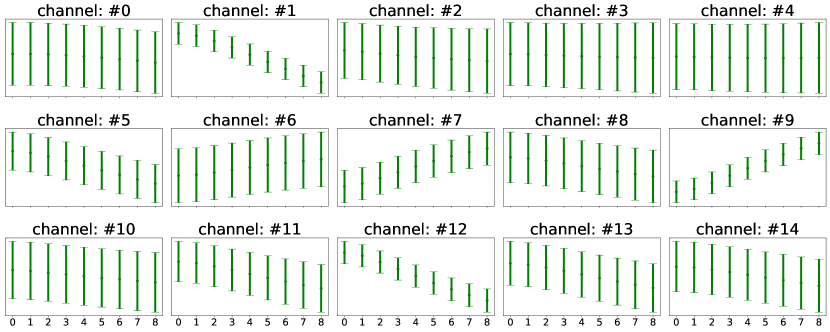
Figure 3: Per-channel mean and variance of intermediate convolution features under different attacking strengths. Features under different attacking strengths undergo a continuous domain transfer.

3 Observation and Motivation

In this section, we first describe the observation and illustrate how we are motivated to develop the Adaptive Feature Alignment method. Then we introduce the details of our proposed method.

3.1 Observation and Motivation

Many recent studies reveal that features of standard/adversarial samples belong to two separate domains  [19, 17], and then developed the dual-BN architecture to process standard/adversarial samples separately. While their methods [19, 17] neglect the inherent variances across adversarial samples of different attacking strengths. Our observational experiments demonstrate that feature statistics of variance attacking strengths undergo a continuous and monotonical domain transfer.

In the observational experiment, we train the Wide-Resnet-28 [6] model on the CIFAR-10 [29] dataset. We adopt the dual-BN architecture proposed in [19] which splits normal and adversarial samples into multiple parallel batch-norm branches. After training, we analyze the statistics of features of various attacking strength on the testing set. Concretely, we visualize the per-channel mean and variance of features from an intermediate convolution layer and results are presented in  Fig. 3.

The results in  Fig. 3 clearly demonstrate that the features are transferring smoothly and monotonically with the rising of attacking strength. This hints us that features of an arbitrary attacking strength can be approximated by a linear combination few "base" intensities. For instance, a medium attacking strength can be represented by a combination of a slight attacking and a strong attacking.

Based on the observational experiment, our motivations are two folds:

1. Features of different attack strengths belong to their respect domains, and use a multi-BN architecture where each BN branch deals with a single attacking strength may result in better aligned features.

2. Features of an arbitrary attacking strength can be represented by a interpolation of two ‘base attacking strengths‘.

Based on above motivation, we design a two-stage framework to train a model that can adaptively align feature for an arbitrary unknown attacking strength. Next, we will detailedly describe the proposed method.

4 Methodology

4.1 Overall Framework

\begin{overpic}[width=433.62pt]{figures/architecture} \put(19.5,12.6){\small{BN${}_{0}$}} \put(19.5,7.0){\small{BN${}_{1}$}} \put(18.2,1.4){\small{BN${}_{k-1}$}} \put(12.0,13.0){$x_{\epsilon=0}$} \put(11.0,2.0){$x_{\epsilon=k-1}$} \put(46.0,11.0){\footnotesize{$\mathcal{L}_{adv}$}} \put(46.0,3.5){\footnotesize{$\mathcal{L}_{CE}$}} \put(65.0,12.5){$x$} \put(65.0,1.5){$x$} \put(71.0,12.3){\footnotesize{BN${}_{0}$}} \put(70.0,1.0){\footnotesize{BN${}_{k-1}$}} \put(2.0,16.0){\normalsize{stage I}} \put(54.0,16.0){\normalsize{stage II}} \put(72.0,16.0){AFA} \put(16.0,-3.0){(a)} \put(72.0,-3.0){(b)} \put(76.5,8.5){\footnotesize{$W_{0}$}} \put(76.5,5.0){\footnotesize{$W_{1}$}} \put(98.0,9.0){\footnotesize{$\mathcal{L}_{CE}$}} \put(69.5,6.5){\small{WG}} \end{overpic}

Figure 4: The overall architecture. (a) In the first stage, we train a dual-branch network where each parallel BN branch corresponds to samples of a specific attacking strength. (b) In the second stage, we drop intermediate BN branches and only keep the outermost branches, i.e., BN₀ and BN_k-1. And the weight generator (WG) in the adaptive feature alignment (AFA) module will generate the fusing weight of the two remaining branches.

The overall architecture of our proposed framework is illustrated in Fig. 4. We denote $I_{\epsilon=k}$ as an adversarial image where $\epsilon$ is the attacking strength, and $I$ represents an image of arbitrary unknown attacking strength. Commonly these attacking methods apply a gradient ascent to the original inputs to obtain adversarial samples. The attacking strength $\epsilon$ is closely related to the gradient magnitude. Specifically, we refer to $I_{\epsilon=0}$ as normal samples without adversarial attacking. Let $x_{\epsilon=k}$ be the convolutional feature extracted from an intermediate layer. Our overall pipeline is extended from the dual-BN architecture that is proposed in [19, 17]. We first extend it into a i.e., $K$-BN ($K\geq 2$) architecture ( Fig. 4 (a)), and then drop some of the BN branches to form the final dual-BN architecture ( Fig. 4 (b)). The training procedure of our framework includes two stages.

In the first stage (Stage I), we train a $K$-BN network with $K$ parallel batch normalization branches and each branch BN${}_{k}(k=0,1,...,K-1)$ deals with samples of specific attacking strength. Note that the attacking strength $\epsilon$ is known to the model so that each sample $x_{\epsilon}$ will only go through the corresponding BN branch according to $\epsilon$.  Fig. 4 (a) demonstrates the training of stage I.

In the second stage (stage II), we drop the intermediate BN branches and only keep two branches corresponding to the strongest and lowest attacking strengths, i.e., BN₀ and i.e., BN_K-1. Then we freeze all the model parameters and train our proposed Adaptive Feature Alignment (AFA) module to automatically adjust fusing weight between BN₀ and BN_K-1. Therefore, the feature of an arbitrary $\epsilon$ can be represented by interpolation of tw ‘base’ attacking strengths.  Fig. 4 (b) illustrates the network structure in stage II. Next, we will detail the proposed ‘adaptive feature alignment’ module.

4.2 Adaptive Feature Alignment

\begin{overpic}[width=325.215pt]{figures/wg.pdf} \put(77.0,6.5){\small{Sigmoid}} \put(10.0,-3.0){\scriptsize{Conv+BN+ReLU}} \put(25.0,12.0){$\times 2$} \put(33.0,-3.0){\scriptsize{Avg Pooling}} \put(56.0,1.0){\scriptsize{Linear}} \put(66.0,12.0){$\times 2$} \end{overpic}

Figure 5: The architecture of the weight generator (WG). The cube represents the ‘Convolution $\rightarrow$ batchnorm $\rightarrow$ ReLU’ sequantial, the trapezoid represents the ‘global average pooling’ and the bar represents the ‘Linear $\rightarrow$ ReLU’ combo. The output is normalized by the sigmoid function.

Let $x$ be the image feature of an arbitrary sample, and BN₀ and BN_k-1 be the remaining BN branches as shown in Fig. 4 (b).

Given the input $x$, the proposed AFA first generates two fusing weights $W_{0},W_{1}$ with a subnetwork termed ‘weight generator’ (WG). The weight generator network consists of 2 sequential Conv-BN-ReLU blocks and then followed by the global average pooling (AVG) and two linear layers. Finally, the output is normalized by the sigmoid function.  Fig. 5 detailly illustrates the architecture of the WG subnetwork. consequently, the fusing weights are output of the weight generator:

$$\begin{split}W_{0}&=\text{WG}(x)\\ W_{1}&=1-W_{0}.\end{split}$$ (1)

Given input $x$ and fusing weights $W_{0},W_{1}$, the out put of AFA $\hat{x}$ is:

$$\hat{x}=W_{0}\cdot\text{BN}_{0}(x)+W_{1}\cdot\text{BN}_{k-1}(x),$$ (2)

where BN₀ and BN_k-1 are the batchnorm operator:

$$\text{BN}(x)=\frac{x-\mu}{\sigma}.$$

4.3 Model Optimization

As aforementioned, the proposed framework contains two training stages. In the first stage, we train a $K$-BN network with both classification loss and the adversarial loss. We use the cross-entropy loss (CE-loss) as the classification loss. Note that our method does not constrain the specific form of adversarial loss. In the second stage, we drop all middle BN-branches and only preserve two outermost ones. Then we fix all network parameters and only optimize the weight generator, as illustrated in Fig. 4 (b). Since the attacking strength is unknown to the model, we use only the classification loss in stage II.

Stage 1: Training basic model. In the first stage, we train the $K$-BN architecture as illustrated in Fig. 4 (a). Note that each BN branch only accepts samples of a specific attacking strength and all other parameters are shared across all samples. Given a sample $x$ with attacking strength $\epsilon$, the loss function can be formulated as:

$$\mathcal{L}_{1}(x_{\epsilon})=\mathcal{L}_{CE}+1(\epsilon>0)\cdot\mathcal{L}_{adv}$$ (3)

where $1(\cdot)$ is a indicator function evaluating to 1 when the condition is true and 0 elsewise. The optimization procedure of stage I is summarized in  algorithm 1, which is extended from  [19].

Stage 2: Training the weight generator. In the second stage, as illustrated in Fig. 4 (b), we drop all other BN branches and only preserve the two outermost branches: BN₀ and BN-_k-1.

Then we place the weight generator (WG) to the end of an intermediate layer to generate adaptive fusing weights $W$. In stage II, we use samples of various attacking strengths to train the WG but the attacking strength is unknown to the model. The only supervision in the second stage is the classification loss, as illustrated in Fig. 4 (b).

Input: The batch of natural samples $x_{c}$ with label $y$, the path quantity $K$, the attack strength vector of each path $\xi$, the adversarial samples generating algorithm $G$, loss function for natural training $L_{c}$, loss function for adversarial training $L_{a}$, the network parameters $\Theta$

iteration number $i\leftarrow 0$, total loss $L_{i}\leftarrow 0$;

while not converged do

       $L_{i}\leftarrow 0$;

       for $k\leftarrow 2$ to $K$ do

             Switch to $k$th path to enable $k$th BN;

             Obtain corresponding attack strength value from the vector $\xi_{k}\leftarrow\xi[k]$;

            Generate adversarial samples with attacking strength $\xi_{k}$ by $x_{a}\leftarrow G(\Theta,x_{c},y,\xi_{k})$;

            Calculate the adversarial loss of $k$th path by $l_{k}\leftarrow L_{a}(\Theta,x_{c},x_{a},y)$;

            Accumulate the total loss $L_{i}\leftarrow L_{i}+l_{k}$;

       end for

      Calculate the normal loss $l_{1}\leftarrow L_{c}(\Theta,x_{c},y)$;

       Accumulate the total loss $L_{i}\leftarrow L_{i}+l_{1}$;

       Compute the gradients of $\Theta$;

       Update the parameters $\Theta$;

      

end while

Output: $\Theta$

Algorithm 1 Training procedure of basic model

5 Experiments

5.1 Experiments Setup

Implementation details. We implement our method with the PyTorch [30] framework. We conduct experiments on three datasets: CIFAR-10 [29], SVHN [5] and tiny-ImageNet [21, 22]. Following several previous works [31, 32, 17], we use the WRN-28-10 [6] network as the backbone for the experiments on CIFAR-10. The WRN-16-8 network is used on SVHN and tiny-ImageNet datasets. We use $K=5$ in all our experiments since we found that $K=5$ achieves a good balance between training efficiency and model performance, as illustrated in our ablation study in Sec. 5.3.

As aforementioned, the training procedure is separated into two stages. On SVHN, the initial learning rates of the two stages are 0.01 and 0.001, respectively. And the initial learning rates on CIFAR and tiny-ImageNet datasets are 0.1 and 0.01, respectively. We train 100 epochs for the first stage and 20 epochs for the second stage. During training, we decay the learning rate with the factor of $0.9$. In the first stage, the learning rate decays at the 75th and the 90th epoch; in the second stage, the learning rate decays at the 10th epoch.

Attacking methods. We adopt 3 adversarial attack algorithms: Fast Gradient Sign Method (FGSM) [8], Projected Gradient Descent (PGD) [1] and C&W attack [24] .

In Tab. 1 and  Tab. 2, we compare our method with other adversarial training methods under the the PGD attack with various attacking strengths, e.g., $\epsilon=0,1,2,4,8$. In  Tab. 3 we test the proposed method under three attacking methods, e.g., FGSM, PGD, and C&W, under a fixed attacking strength of $\epsilon=8$.

Adversarial training baselines. As demonstrated in Eq. 3, our method does not constrain the specific form of the adversarial loss function. Therefore, our method can be integrated with many adversarial training methods. In our experiments, we use 4 adversarial training methods as baselines: PGD-AT [1], TRADES [2], IAT [3] and MART [4].

5.2 Quantitative Comparisons

We compare our proposed method with several recent methods, i.e., OAT [17],PGD-AT [1], TRADES [2], IAT [3], and MART [4]. Quantitative results on CIFAR-10 [29], SVHN and tiny-ImageNet [22] datasets are summarized in Tab. 1 and Tab. 2, respectively.

Method	SVHN						CIFAR-10
	$\epsilon=0$	$\epsilon=1$	$\epsilon=2$	$\epsilon=4$	$\epsilon=8$	Avg	$\epsilon=0$	$\epsilon=1$	$\epsilon=2$	$\epsilon=4$	$\epsilon=8$	Avg
Standard	96.5	73.7	39.1	6.5	0.2	43.2	95.2	30.5	3.0	0.0	0.0	25.7
1-7[1pt/2pt] PGD-AT	93.0	83.7	77.4	68.3	46.5	73.8	86.9	81.5	78.5	68.8	46.2	72.4
PGD-AT+ ours	98.1	93.1	87.8	75.4	46.4	80.0	95.8	87.0	83.9	72.6	50.0	77.9
1-13[1pt/2pt] TRADES	85.3	81.8	77.6	70.9	53.2	73.8	83.2	80.5	77.6	71.3	53.8	73.3
TRADES+ ours	97.0	89.0	88.4	77.6	54.2	81.4	95.4	86.8	82.7	72.1	52.6	77.9
1-13[1pt/2pt] IAT	95.9	83.3	78.2	63.5	40.5	72.3	92.9	88.3	84.4	73.5	46.2	77.0
IAT+ours	97.4	91.6	87.9	75.9	42.3	79.0	96.1	86.2	81.7	73.7	46.2	76.7
1-13[1pt/2pt] MART	82.5	75.4	65.5	58.9	58.2	68.1	83.6	81.0	78.2	72.3	55.3	74.1
MART+ ours	97.0	93.5	88.5	78.4	58.7	83.2	95.9	84.3	84.2	73.5	56.1	78.8

Table 1: Adversarial accuracy on SVHN and CIFAR-10 datasets. Our proposed method consistently outperforms baseline adversarial training methods with a clear margin.

Performance on SVHN and CIFAR-10. We first test the proposed method as well as other adversarial training methods on two small datasets: SVHN and CIFAR-10. Results in  Tab. 1 reveal that: 1) our method outperforms the standard model in terms of standard accuracy ($\epsilon=0$), this is mainly due to the dual-BN architecture [19]. 2) Our proposed method consistently improve the adversarial accuracy based on three adversarial training methods. Especially, our method achieves high adversarial accuracy under a variety of attacking strengths, we believe this this mainly due to the proposed ‘adaptive feature align’ that can automatically align features according to the attacking strength.

Method	Acc under different $\epsilon$
	0	1	2	4	8	Avg
Standard	63.5	6.7	1.0	0.2	0.0	14.3
1-7[1pt/2pt] PGD-AT	50.4	44.6	38.8	28.0	13.5	35.1
PGD-AT+ ours	64.5	46.8	35.3	28.1	13.8	37.7
1-7[1pt/2pt] TRADES	42.1	38.2	34.0	26.6	15.1	31.2
TRADES+ ours	62.5	47.9	39.2	26.7	15.1	38.3
1-7[1pt/2pt] MART	41.0	37.3	33.6	27.1	16.4	31.1
MART+ ours	63.9	44.8	38.6	27.8	16.5	38.3

Table 2: Adversarial accuracy on the tiny-ImageNet dataset.

Performance on tiny-ImageNet. The comparison results on tiny-ImageNetNet are reported in  Tab. 2. The results are consistent with the previous conclusion, which shows a stable promotion of our method on a larger scale dataset.

Other attacking methods. In this experiment, we compare we evaluate the adversarial accuracy under other attacking methods, e.g., PGD [1], FGSM  [8] and C&W [24]. The attacking strength is fixed to $\epsilon=8$. Results are summarized in Tab. 3. Besides, we provide the performance of query-based attacking, e.g., square attack [33], in the supplementary material.

Method	Attacking methods					Black-box attacking
	std.	PGD	FGSM	C&W	PGD+Ada.	0	1	2	4	8	Avg
Standard	95.2	0.0	24.2	0.0	-	95.2	0.0	24.2	0.0	-
1-6[1pt/2pt] PGD-AT	86.9	46.2	56.1	45.3	-	86.9	85.2	83.1	78.2	66.8	80.0
PGD-AT+ ours	95.8	50.0	81.1	48.3	48.2	95.8	94.6	90.5	91.9	67.9	88.1
1-12[1pt/2pt] TRADES	83.2	53.8	64.6	52.5	-	83.2	81.5	79.0	74.1	65.3	76.6
TRADES+ ours	95.4	52.6	80.3	51.0	52.2	95.4	94.7	92.7	82.4	65.9	86.2
1-12[1pt/2pt] IAT	92.9	46.2	65.7	43.4	-	92.9	91.2	88.7	84.5	71.8	85.8
IAT+ours	96.1	46.2	80.6	43.5	46.1	96.1	95.2	93.6	87.0	74.0	89.2
1-12[1pt/2pt] MART	83.6	55.3	64.3	53.4	-	83.6	82.0	80.0	76.1	66.0	77.6
MART+ ours	95.9	56.0	81.3	53.6	55.6	95.9	95.3	93.4	83.7	67.7	87.2

Table 3: Left: adversarial accuracies under 3 different attacking methods and adaptive attack (PGD+Ada). Right: adversarial accuracies with black-box attacking. Our method is more robust against adversarial attacks compared to the adversarial training baselines.

The results in Tab. 3 tell that our method consistently outperforms the competitors under various attacking methods and attacking strengths. Specifically, under the FGSM attack, our method surpasses others with a significant margin and the average performance improvement is nearly 15%.

Adaptive attack. Adaptive attacks [34] are specifically crafted to compromise a proposed approach form a crucial component of adversarial evaluation. We test our method on the adaptive attack setting by exposing the fusing weight, i.e., $W_{0}$, to the attacker. Concretely, we setup PGD by combining the cross-entropy loss for classification outputs and the binary-cross entropy (BCE) loss for weight generator to jointly perform gradient ascent. We test 7 different loss weights between CE and BCE (10:1, 5:1, 2:1, 1:1, 1:2, 1:5, 1:10) and report the best attacking results (worst adversarial accuracies) in the last column of Tab. 3. More details about the settings of adaptive attack are presented in the supplementary material.

The results of adaptive attacking are in Tab. 3 (the ‘PGD+Ada’ column). The performance gap between PGD and PGD+Adv is marginal, revealing that the proposed WG module is somehow robust against adaptive attacking.

Black-box robustness. Black-box attacks generate adversarial samples by attacking a surrogate model which has a similar structure with the defense model and is trained on with similar tasks. Following setting in  [4, 35], we use ResNet-50 model as the surrogate model and it is trained on the CIFAR-10 dataset. Then we generate adversarial samples by attacking the surrogate model and test the performance of the defense model.

As shown in Tab. 3 (right), our method achieves better performance compared to adversarial training baselines under black-box attacking. This reveals that our method alleviates the ‘obfuscated gradients’ effect. It can be verified by the following evidence [36, 2]: (1) our method has higher accuracy under weak attacks (e.g., FGSM) than strong attacks (e.g., PGD). (2) our method has higher accuracy under black-box attacks than white-box attacks.

5.3 Ablation Study

In this section, we do several ablation experiments on the CIFAR-10 dataset to verify& interpret our proposed framework.

Choice of $K$. Here we ablate the choice of $K$ when training the $K$-BN architecture in stage I as illustrated in Fig. 4. Results in Tab. 4 reveals that the model benefits from a larger and the performance saturates at $K\geq 5$. For the compromise between performance and efficiency, we use $K=5$ in our experiments.

Relationship between fusion weight and $\epsilon$ To further probe the behavior of AFA, we analyze the relationship between fusion weights ($W_{1}$) and the attacking strength ($\epsilon$). Specifically, we train a ResNet-34 model on CIFAR-10 to generate adversarial samples of random attacking strengths.

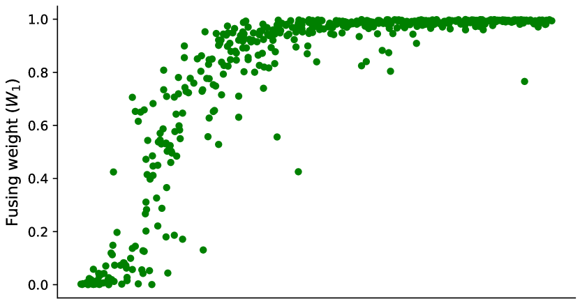
Figure 6: Relationship between fusion weight $W_{1}$ and $\epsilon$. With the rising of $\epsilon$, $W_{1}$ increases, the features are biased towards the adversarial BN branch, i.e., BN_k-1.

# BNs	Acc under different $\epsilon$
	0	1	2	4	8	Avg
$K=2$	95.0	85.1	82.2	70.4	48.1	76.2
$K=3$	95.5	86.7	83.2	72.3	48.6	77.3
$K=5$	95.8	87.0	83.9	72.6	50.0	77.9
$K=9$	95.6	87.2	84.5	72.9	50.4	78.1

Table 4: Ablation of the number of BN branches $K$ in stage I. In general, the performance improves with the raising of $K$.

As shown in Fig. 6, the AFA is biased towards the the adversarial branch (BN_K-1) when the attacking strength rises, as evidenced by the increase of $W_{1}$. This nonlinear mapping is automatically learned by the weight generator.

6 Conclusion

In this paper, we proposed a simple yet effective framework for adversarial training. We observed that the feature statistics of adversarial features transfer smoothly with the change of attacking strength. Based on the observation, we proposed an adaptive feature fusion framework to automatically align features for inputs of arbitrary attacking strength. Compared to previous works, our method can handle input of different attacking strengths on the fly with a single model, showing its potential in real-world applications. We applied the proposed method to several recent adversarial training methods,  e.g., FGSM, PGD, TRADES, and MART, and tested the performance on SVHN, CIFAR-10, and tiny-ImageNet datasets. Extensive experiments demonstrated that our method improves the adversarial training baselines with a considerable margin, under a wide range of attacking strengths.

References

- [1] Aleksander Madry, Aleksandar Makelov, Ludwig Schmidt, Dimitris Tsipras, and Adrian Vladu. Towards deep learning models resistant to adversarial attacks. In Int. Conf. Learn. Represent., 2017.
- [2] Hongyang Zhang, Yaodong Yu, Jiantao Jiao, Eric P Xing, Laurent El Ghaoui, and Michael I Jordan. Theoretically principled trade-off between robustness and accuracy. 2019.
- [3] Alex Lamb, Vikas Verma, Juho Kannala, and Yoshua Bengio. Interpolated adversarial training: Achieving robust neural networks without sacrificing too much accuracy. In Proceedings of the 12th ACM Workshop on Artificial Intelligence and Security, pages 95–103, 2019.
- [4] Yisen Wang, Difan Zou, Jinfeng Yi, James Bailey, Xingjun Ma, and Quanquan Gu. Improving adversarial robustness requires revisiting misclassified examples. In Int. Conf. Learn. Represent., 2019.
- [5] Yuval Netzer, Tao Wang, Adam Coates, Alessandro Bissacco, Bo Wu, and Andrew Y Ng. Reading digits in natural images with unsupervised feature learning. 2011.
- [6] Sergey Zagoruyko and Nikos Komodakis. Wide residual networks. arXiv preprint arXiv:1605.07146, 2016.
- [7] Christian Szegedy, Wojciech Zaremba, Ilya Sutskever, Joan Bruna, Dumitru Erhan, Ian Goodfellow, and Rob Fergus. Intriguing properties of neural networks. In Int. Conf. Learn. Represent., 2013.
- [8] Ian J Goodfellow, Jonathon Shlens, and Christian Szegedy. Explaining and harnessing adversarial examples. 2015.
- [9] Omkar M Parkhi, Andrea Vedaldi, and Andrew Zisserman. Deep face recognition. 2015.
- [10] Mariusz Bojarski, Davide Del Testa, Daniel Dworakowski, Bernhard Firner, Beat Flepp, Prasoon Goyal, Lawrence D Jackel, Mathew Monfort, Urs Muller, Jiakai Zhang, et al. End to end learning for self-driving cars. Adv. Neural Inform. Process. Syst., 2016.
- [11] Chuan Guo, Mayank Rana, Moustapha Cisse, and Laurens van der Maaten. Countering adversarial images using input transformations. In Int. Conf. Learn. Represent., 2018.
- [12] Cihang Xie, Jianyu Wang, Zhishuai Zhang, Zhou Ren, and Alan Yuille. Mitigating adversarial effects through randomization. In Int. Conf. Learn. Represent., 2018.
- [13] Jacob Buckman, Aurko Roy, Colin Raffel, and Ian Goodfellow. Thermometer encoding: One hot way to resist adversarial examples. In Int. Conf. Learn. Represent., 2018.
- [14] Cihang Xie, Yuxin Wu, Laurens van der Maaten, Alan L Yuille, and Kaiming He. Feature denoising for improving adversarial robustness. In IEEE Conf. Comput. Vis. Pattern Recog., pages 501–509, 2019.
- [15] David Stutz, Matthias Hein, and Bernt Schiele. Disentangling adversarial robustness and generalization. In IEEE Conf. Comput. Vis. Pattern Recog., pages 6976–6987, 2019.
- [16] Dimitris Tsipras, Shibani Santurkar, Logan Engstrom, Alexander Turner, and Aleksander Madry. Robustness may be at odds with accuracy. Int. Conf. Learn. Represent., 2019.
- [17] Haotao Wang, Tianlong Chen, Shupeng Gui, Ting-Kuei Hu, Ji Liu, and Zhangyang Wang. Once-for-all adversarial training: In-situ tradeoff between robustness and accuracy for free. In Adv. Neural Inform. Process. Syst., 2020.
- [18] Andrew Ilyas, Shibani Santurkar, Dimitris Tsipras, Logan Engstrom, Brandon Tran, and Aleksander Madry. Adversarial examples are not bugs, they are features. In Adv. Neural Inform. Process. Syst., pages 125–136, 2019.
- [19] Cihang Xie, Mingxing Tan, Boqing Gong, Jiang Wang, Alan L Yuille, and Quoc V Le. Adversarial examples improve image recognition. In IEEE Conf. Comput. Vis. Pattern Recog., pages 819–828, 2020.
- [20] Hao Wang, Hao He, and Dina Katabi. Continuously indexed domain adaptation. 2020.
- [21] Jia Deng, Wei Dong, Richard Socher, Li-Jia Li, Kai Li, and Li Fei-Fei. Imagenet: A large-scale hierarchical image database. In CVPR, pages 248–255. Ieee, 2009.
- [22] https://tiny-imagenet.herokuapp.com/.
- [23] Alexey Kurakin, Ian Goodfellow, and Samy Bengio. Adversarial machine learning at scale. 2017.
- [24] Nicholas Carlini and David Wagner. Towards evaluating the robustness of neural networks. In 2017 ieee symposium on security and privacy (sp), pages 39–57. IEEE, 2017.
- [25] Florian Tramèr, Alexey Kurakin, Nicolas Papernot, Ian Goodfellow, Dan Boneh, and Patrick McDaniel. Ensemble adversarial training: Attacks and defenses. Int. Conf. Learn. Represent., 2018.
- [26] Ziang Yan, Yiwen Guo, and Changshui Zhang. Deep defense: Training dnns with improved adversarial robustness. In Adv. Neural Inform. Process. Syst., pages 419–428, 2018.
- [27] Moustapha Cisse, Piotr Bojanowski, Edouard Grave, Yann Dauphin, and Nicolas Usunier. Parseval networks: Improving robustness to adversarial examples. ICML, 2017.
- [28] Farzan Farnia, Jesse M Zhang, and David Tse. Generalizable adversarial training via spectral normalization. arXiv preprint arXiv:1811.07457, 2018.
- [29] Alex Krizhevsky, Geoffrey Hinton, et al. Learning multiple layers of features from tiny images. 2009.
- [30] Adam Paszke, Sam Gross, Francisco Massa, Adam Lerer, James Bradbury, Gregory Chanan, Trevor Killeen, Zeming Lin, Natalia Gimelshein, Luca Antiga, et al. Pytorch: An imperative style, high-performance deep learning library. In Adv. Neural Inform. Process. Syst., pages 8026–8037, 2019.
- [31] Gavin Weiguang Ding, Yash Sharma, Kry Yik Chau Lui, and Ruitong Huang. Mma training: Direct input space margin maximization through adversarial training. In Int. Conf. Learn. Represent., 2019.
- [32] Jianyu Wang and Haichao Zhang. Bilateral adversarial training: Towards fast training of more robust models against adversarial attacks. In Int. Conf. Comput. Vis., pages 6629–6638, 2019.
- [33] Maksym Andriushchenko, Francesco Croce, Nicolas Flammarion, and Matthias Hein. Square attack: a query-efficient black-box adversarial attack via random search. In European Conference on Computer Vision, pages 484–501. Springer, 2020.
- [34] Nicholas Carlini, Anish Athalye, Nicolas Papernot, Wieland Brendel, Jonas Rauber, Dimitris Tsipras, Ian Goodfellow, Aleksander Madry, and Alexey Kurakin. On evaluating adversarial robustness. arXiv preprint arXiv:1902.06705, 2019.
- [35] Yisen Wang, Xingjun Ma, James Bailey, Jinfeng Yi, Bowen Zhou, and Quanquan Gu. On the convergence and robustness of adversarial training. In ICML, volume 1, page 2, 2019.
- [36] Anish Athalye, Nicholas Carlini, and David Wagner. Obfuscated gradients give a false sense of security: Circumventing defenses to adversarial examples. ICML, 2018.