![[Uncaptioned image]](/html/2105.15154/assets/x2.png)
![]()
|
|
CO2-driven diffusiophoresis and water cleaning: similarity solutions for predicting the exclusion zone in a channel flow† |
| Suin Shim,a,∗ Mrudhula Baskaran,b Ethan H. Thai,c and Howard A. Stonea,‡ | |
|
|
We investigate experimentally and theoretically diffusiophoretic separation of negatively charged particles in a rectangular channel flow, driven by CO2 dissolution from one side-wall. Since the negatively charged particles create an exclusion zone near the boundary where CO2 is introduced, we model the problem by applying a shear flow approximation in a two-dimensional configuration. From the form of the equations we define a similarity variable to transform the reaction-diffusion equations for CO2 and ions and the advection-diffusion equation for the particle distribution to ordinary differential equations. The definition of the similarity variable suggests a characteristic length scale for the particle exclusion zone. We consider height-averaged flow behaviors in rectangular channels to rationalize and connect our experimental observations with the model, by calculating the wall shear rate as functions of channel dimensions. Our observations and the theoretical model provide the design parameters such as flow speed, channel dimensions and CO2 pressure for the in-flow water cleaning systems. |
‡hastone@princeton.edu
1 Introduction
Diffusiophoresis is the spontaneous motion of colloidal particles under a solute concentration gradient. Since the first recognition 1, 2, the phenomenon has been widely studied theoretically and experimentally 3, 4, 5, 6, 7, 8, 9, 10, 11, 12, 13, 15, 16, 17, 14, 18, 19. When the solute is an electrolyte, the net motion of particles has electrophoretic and chemiphoretic contributions, induced by, respectively, the diffusivity difference(s) among the ions and the osmotic pressure gradient near the particle surface 5.
Various experimental investigations have been reported for the diffusiophoresis of micron-sized particles, either in the presence or absence of liquid flow 12, 13, 22, 14, 18, 19, 20, 21. Recently, it has been demonstrated that dissolution of gas can drive diffusiophoresis of charged particles 23, 22, 25, 26, 27, 24. In particular, CO2 was used in several earlier studies due to its ubiquity and importance in many applications. From a transport perspective the most important feature of CO2 as a means for driving diffusiophoresis is that it undergoes rapid dissolution and reaction in water, creating H+ and HCO ions by the dissociation of H2CO3. These ions have a large difference in their diffusivities with m2s-1 and m2s-1, leading to a large diffusion potential and diffusiophoretic mobility of suspended charged particles 23, 22, 25, 26, 27, 24.
As the nature of diffusiophoresis allows moving charged particles with an imposed directionality, it has been suggested for water cleaning. In our previous work 26, we demonstrated in a Hele-Shaw geometry that bacterial cells can be excluded from a region near a CO2 source by CO2-driven diffusiophoresis. Shin et al.22, Lee et al.21, and Seo et al28, demonstrated removing particles from water by diffusiophoretic exclusion of particles, using a CO2 gas chamber or Nafion as the sources of ions, respectively, in a configuration where the solute gradient is created perpendicular to the liquid flow. The main mechanism for such a configuration is that either a particle free zone or an accumulation zone forms near the walls depending on the diffusiophoretic mobility and the direction of the concentration gradient. However, the reported experiments use one or two geometrical conditions (in each study), and we sought to understand what could be achieved in larger scales with the analogous exclusion zone formation.
To better understand the transport process in such in-flow water cleaning systems, and to discuss scale-up possibilities, mathematical models are needed. A simple increase in the geometry cannot be applied for effective scale-up of the system due to the nonlinearity of the diffusiophoresis, possible transitions from laminar to turbulent flows, and other effects (e.g. gravity) that influence the system as the length scale increases. For example, CO2 dissolved water is denser than normal water, so a simple increase in the length scale will cause buoyancy effects that complicate the flow and the motion of the particles. In such case a different design is necessary.
In this paper, we are interested in a channel flow configuration where the driving source of diffusiophoretic water cleaning is dissolved CO2, and the concentration gradient is perpendicular to the flow 22. Through the detailed investigation of the steady-state flow and the particle exclusion zone using both theory and experiments, we identify important parameters that directly affect the scalability of the system and the exclusion zone. In particular, we apply a shear flow approximation to the near-wall region in the channel flow, and develop similarity solutions for the distribution of ions and particles. Then with control experiments and numerical calculations considering the effect of channel geometry we identify parameters that influences the size of the exclusion zone, which directly affects the efficiency of the water cleaning. Our goal is not to provide an optimal solution or the most efficient channel design. Rather, we try to sort out the important system parameters to apply to the device design process.
2 Formation of the particle exclusion zone in channel flow
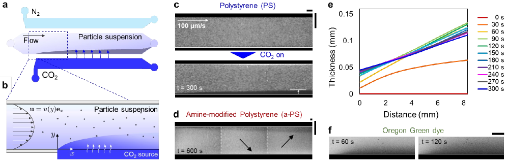
We create a concentration gradient of CO2 in a channel flow by placing a CO2 channel and the N2 channel adjacent to the liquid channel. The permeable PDMS membranes between the channels (thickness m) let the gases dissolve into the liquid channel (see Figure 1(a)). As a result, a steady state concentration gradient of CO2 is set up in the liquid channel as described in Figure 1(a,b). In the liquid channel, a particle suspension (polystyrene; 0.03 vol in DI water) flows into the channel at a constant mean flow velocity. As a result of the CO2 concentration gradient which leads to the ion (H+ and HCO) concentration gradients across the channel, the charged particles either form an exclusion zone or accumulate near the CO2-side boundary depending on the surface charge of the particles. Negatively charged polystyrene (PS) particles form a particle-free zone near the CO2-side wall as shown in Figure 1(c) while positively charged amine-modified polystyrene (a-PS) particles accumulate (Figure 1(d)). Details of the experimental setup is described in the Materials and Methods section. In this study, we focus on the particle exclusion zone formation near the CO2-side boundary. Figure 1(e) shows the measured shape of the particle exclusion zone at different times when negatively charged particles flow into the channel at a mean speed m/s. The boundary of the exclusion zone is plotted versus distance along the channel, which is measured from the CO2 inlet position (Figure 1(a,b)). We note that some time after the CO2 stream is turned on, the particle exclusion zone grows then reach a steady-state as shown in Figure 1(e) (a longer time experiment is presented in the SI). The nonzero thickness near is due to the CO2 diffusion in the PDMS walls, which makes the influx of CO2 occur from further upstream. The diffusion of CO2 in the liquid channel can be visualized with a pH-sensitive dye (Oregon Green 488, Figure 1(f)).
The diffusiophoretic velocity of particles under the ion concentration gradient is written as
| (1) |
where is the diffusiophoretic mobility of the particles under a concentration gradient of a z:z electrolyte 5;
| (2) |
Here , , , , and are, respectively, the dielectric permittivity of the solution, dynamic viscosity of the solution, Boltzmann’s constant, absolute temperature and the zeta potential of the particle. is the diffusivity difference factor, which determines the strength of the local electric field induced by the difference in diffusivities of the ions.
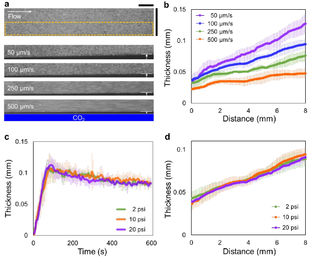
To obtain initial understanding of the system, we controlled the flow rate in the liquid channel and varied the CO2 pressure. In the channel flow, the shape of steady-state exclusion zone can be varied by changing the flow speed (Figure 2(a,b)). For faster flows, we obtain thinner exclusion zones simply because the advection and diffusion of CO2 and ions are perpendicular to each other, and the diffusiophoresis has diffusive feature (note that the diffusiophoretic mobility has a dimension ).
In the experiments where CO2 pressure was varied, we observed that there was not much change in the shape of the exclusion zone. For three different CO2 pressures (2, 10 and 20 psi) applied to the CO2 stream, both time evolution (Figure 2(c)) and the steady state shape (measured at s, Figure 2(d)) of the exclusion zone were not affected. We interpret that this no-CO2-pressure-dependence is due to the fast reaction and the logarithmic feature of diffusiophoresis. From equation (1), we can estimate the particle velocity by an order of magnitude estimate , where is the width of the channel over which the ion concentration gradient is formed. This supports our observation that CO2 pressure did not affect the shape of particle exclusion zone. The scaling analysis will not apply to situations where the ion concentration is either very small or very large, which is considered outside the range of our experiments.
Our initial investigation of the particle exclusion zone with various flow speeds and CO2 pressures tells us that having slower flow is good for having a larger exclusion zone, and we only need a moderate amount of CO2 to achieve such an exclusion zone. However, this is not enough information for scale-up of the system. For example, slower flow will result in a smaller amount of clean liquid collected at the outlet, which lowers the system efficiency. Therefore, we investigate the system in more detail with a mathematical model.
3 Steady-state, 2D model with a shear flow approximation
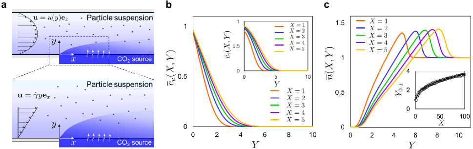
Consider a fully developed flow of a particle suspension in a rectangular microfluidic channel. If CO2 dissolves into the liquid from one wall as decribed in Fig. 3(a), we expect to achieve diffusiophoresis of particles induced by an ion concentration gradient in the channel created by the reaction 23, 22, 26, 25, 27, 24
| (3) |
Assume a 2D pressure driven flow with flow velocity u ex, then the reaction-diffusion equation for dissolved CO2 and dissociated ions can be written as 26, 24
| (4) | ||||
| (5) |
where , are concentrations of CO2 and ions, and and are, respectively, diffusivity of CO2 ( m2/s) and the ambipolar diffusivity of the ions. s-1 and L/mols are forward and reverse reaction rate constants 29, 30, 31. The equations can be solved numerically with appropriate boundary and initial conditions for . For long times we neglect the time derivative to obtain the steady state concentration field of the ions.
Here we want to seek for solutions for a simplified problem within a small length scale. Consider CO2 dissolution and dissociation within small enough that the concentration distribution of dissolved CO2 does not extend across the entire channel width. Then the region of interest is a thin layer near the wall where CO2 is supplied to the liquid phase. Then we can assume that the liquid flow is simply a shear flow with velocity u ex where is shear rate (Fig. 3(a)-bottom panel), and apply the boundary layer approximation to further calculations, which is well-known as the Lévêque approximation in the Chemical Engineering literature. 32.
Now consider steady state reaction-diffusion equations for CO2 and ions in this near-wall region;
| (6) | ||||
| (7) |
Boundary conditions are, , , and , where is the equilibrium concentration of CO2 under the applied CO2 pressure so that ( is Henry’s Law constant). Note that the ions satisfy a zero flux condition at the CO2-side boundary, and also note that under chemical equilibrium , where is the saturation concentration of ions under the applied gas pressure . Equations (6) and (7) can be nondimensionalized with , , and . The nondimensional diffusion-reaction equations are
| (8) | ||||
| (9) |
where is the nondimensional ambipolar diffusivity. The nondimensional boundary conditions are then, , , and . We note that is dimensionless, and for s-1, . Equations (8) and (9) were solved with Matlab and plotted versus for different values in Figure 3(b). The plots show that both CO2 and ions diffuse into the channel (toward larger ) as the liquid flows downstream (increasing ). Note that the CO2 has a constant pressure (and so the concentration) condition at the boundary and the solutions for ions show zero-flux condition at the boundary. Using the concentration of ions and the diffusiophoretic velocity of particles, now we can solve for the particle distribution in the channel also under the shear flow approximation.
The 2D unsteady advection-diffusion equation for particles of concentration is
| (10) |
where and are, respectively, the and components of diffusiophoretic velocity . For small and , we can apply the shear flow approximation to the particle equation. Note that under the boundary layer approximation, we can neglect the diffusiophoresis in the direction for . This is valid for most experimental situations so we keep the condition for further calculations. Then we obtain a steady-state equation for particles,
| (11) |
Boundary conditions are, and at , where is the unperturbed particle concentration.
The equation can be nondimensionalized with , and , and thus
| (12) |
where and . Equation (12) is solved and the solution is plotted versus for different positions along the channel in Figure 3(c). Note that the solutions show zero particle concentration region near which indicates the particle exclusion zone. We calculated the value of where , then plotted this location versus (inset of Figure 3(c)). This plot shows an approximate shape of the steady-state particle exclusion zone obtained from the model calculation. For the shear rate s-1, the nondimensional thickness of exclusion zone yields a dimensional length scale is m, which provides a reasonable estimate of a typical length scale of exclusion zone thickness.
Performing numerical calculation of the partial differential equations (PDEs) provides a good estimate of the particle exclusion zone, but we can further simplify our equations. From the form of the equation, we can deduce a similarity variable and analyze the system with a set of ordinary differential equations (ODEs).
4 Similarity solutions for predicting particle exclusion zone
From the structure of equation (8), we can consider a similarity variable and find a similarity solution . Substituting with in equation (8), we get
| (13) |
Finding that satisfies gives , and thus equation (13) becomes
| (14) |
Since for small (note that for s-1), the reaction term can be neglected. Therefore, we solve an ODE
| (15) |
with the boundary conditions and . This is a similarity transform of the well-known Lévêque problem, and the solution to equation (15) is
| (16) |
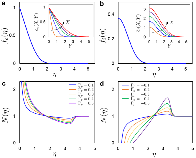
Here is the Gamma function and is the incomplete Gamma function, i.e. . The solution (16) is plotted in Figure 4(a). The inset of Figure 4(a) shows the solutions to the Lévêque problem plotted versus at different values of . The plots show the diffusion of CO2 into the channel starting from the boundary ().
The same analysis can be applied to the concentration of ions near the boundary. For equation (9), we can find a similarity solution by defining with . Substituting this into equation (9), we obtain
| (17) |
where the term for small . Therefore,
| (18) |
and the boundary conditions are and . The ion concentration satisfies no-flux condition at the CO2-side boundary. This equation shows that the ion concentration depends on the CO2 concentration by the forcing term . Equation (18) is solved and plotted in Figure 4(b). The inset of Figure 4(b) is the plot of versus at different values of . For increasing , the ions created by the reaction diffuse into the channel.
Finally, we can consider the particle distribution near the CO2 boundary where CO2 enters. Define and substitute into equation (12) we obtain
| (19) |
The boundary conditions are, at and . Under typical experimental conditions, , and thus we can neglect the particle diffusion. As a result, we solve a first-order ODE for ,
| (20) |
with a boundary condition . Both for positively charged () and negatively charged particles (), the equation (20) is solved and plotted versus in Figure 4(c,d) with five different magnitudes of the mobility . Solutions to the full equation (19) are plotted in the SI. For positively charged particles (Figure 4(c)), there is accumulation (increase in particle concentration) near the boundary , and the particle accumulation is enhanced for larger mobilities. For negatively charged particles (Figure 4(d)), we note that for each value of diffusiophoretic mobility, there is a critical value of below which the particle concentrations are effectively zero. We call this cutoff value . In our experiments, the diffusiophoretic mobility of the negatively charged polystyrene particles corresponds to , and the critical value .
In our model calculations, provides a direct measure for the exclusion zone profile by its definition. From the definition of the similarity variable, we note that
| (21) |
where and are, respectively, the dimensional and nondimensional coordinates of the boundary of the particle excluzion zone. Therefore, we can write the shape of the boundary in coordinates as
| (22) |
where is a prefactor that reflects the details of the three-dimensional flow.
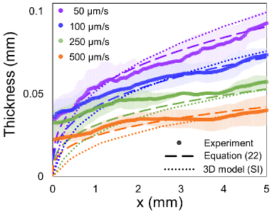
With the experiment presented in Figure 2, we compare the steady-state exclusion zone profile with the equation (22) in Figure 5. In section 4, we used the small condition to obtain equation (15). For s-1 and s-1 the condition becomes cm, and thus we compare the experimental data with the equation (22) up to mm. The wall shear rate values were estimated based on the height-averaged velocity (presented in the next section) in a channel with the width and height, respectively, mm and m. In Figure 5, the curves for equation (22) represent the calculations with wall shear rate values and s-1, corresponding to the mean flow speeds m/s. The steady-state exclusion zone match the scaling equation (22) well with the choice of . Different channel geometries may require different fitting parameters. We also obtained the exclusion zone boundary from three-dimensional (3D) model calculation (details are included in the SI sections 6 and 7); and the scaling analysis, experiments and a 3D model show good agreement near the inlet of the channel (Figure 5). Note that the 3D calculation is not the main focus of the study so we only include it in the SI.
In the experimental situations, the value of is usually a constant if the particle zeta potential and so the mobility are constant. Therefore, we conclude with the relation that the thickness of particle exclusion zone . This means that the size of the particle exclusion zone is determined by the wall shear rate. The trend was recognized by Lee et al.21 (; is the exclusion zone thickness and is the mean flow speed) in the numerical simulations. In our article, we further study the rectangular channel flow to calculate the wall shear rate, and examine the effect of channel geometry and validity of the power law under multiple conditions.
So far we have confirmed with the experiments and the theoretical model based on a shear flow approximation that the flow speeds control the exclusion zone thickness. However, changing flow speed (or the volumetric flow rate) also changes the number of particles per volume that are excluded from the boundary. Therefore, in terms of “water cleaning” experiment, changing the flow rate to test the effect of shear rate on particle exclusion is not a single-parameter control. Thus in the next section, we study the details of flow structure in a rectangular microfluidic channel, and show how the wall shear rate can be varied in such a system without changing the flow speed. In that way, we can test only the effect of shear rate on the size of the particle exclusion zone, without perturbing the number of excluded particles per volume.
5 Wall shear rate in a rectangular channel
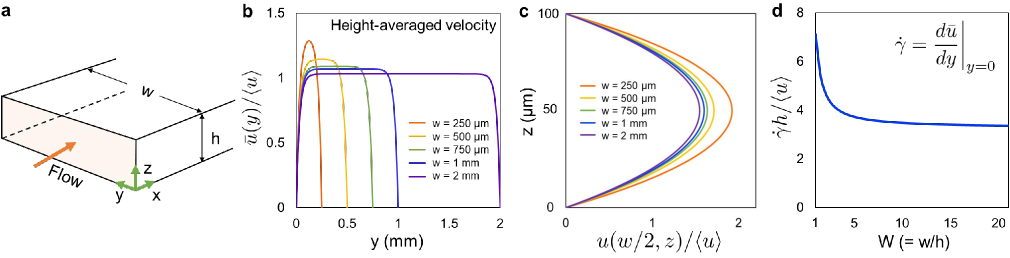
In this section, we investigate the flow structure to find important parameters for controlling the shear rate in a rectangular channel. Consider a channel with the width, height, and length, respectively , , and . We define the axes from a corner of the channel (Figure 6(a)), , , and in the flow, width, and height directions, so that the flow velocity can be written as
| (23) | ||||
where , , and is the mean flow speed. Note that the series solution is first obtained for the coordinate system defined along the centerline of the channel, then shifted by and (see SI for details).
In the experiments, the exclusion zone forms from one side wall, which means that we are observing the height-averaged view of the system. Therefore, we consider the height-averaged velocity profile to obtain the wall shear rate at and simplify the analysis to a two-dimensional flow. The height-averaged velocity is (see SI for details)
| (24) | ||||
where . The equation (24) is normalized by and calculated for different values of channel widths ( and mm) and m, and plotted versus in Figure 6(b). Also, the velocity profile viewed from the side wall, along the centerline, () is calculated and plotted for channels with different widths (Figure 6(c)). For , the flow velocity is almost uniform across the width of the channel, except for the small region near the walls.
Next we calculate the shear rate at the wall ( or ) using the height-averaged velocity :
| (25) | ||||
Note that if we maintain the mean flow speed and the channel height constant, the aspect ratio of the channel is the main parameter that can vary the shear rate at the wall. The normalized shear rate is plotted versus in Figure 6(d). This calculation shows that for the same mean flow velocity and the channel height, we can tune the wall shear rate simply by changing the width of the channel. For smaller , the shear rate is higher. We also note that (SI) the shear rates at and are smaller for larger , which means that for the same mean flow velocity and , we obtain lower shear rates on all four walls in the channels with larger widths.
6 Exclusion zone formation in the channels with various geometries
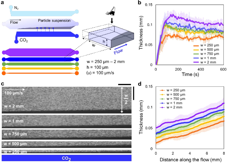
From the previous sections, we obtained the relation for the thickness of exclusion zone () and calculated the wall shear rate as a function of channel dimensions. Motivated by the shear rate calculations, we performed control experiments with the rectangular channels with the height m and different widths and mm (Figure 7(a)). We observe the particle exclusion zone near the CO2-side boundary at a fixed mean flow speed m/s. CO2 and N2 pressures were maintained at, respectively, 10 psi and 1.5 psi. 300 seconds after the CO2 flow is on, we obtain different exclusion zones in the channels of different widths (Figure 7(b-d)).
As predicted from the calculations, the shear rate is smaller for larger channels with fixed values of and , and thus we observe larger exclusion zones in the channels with larger width. We measured the time evolution of particle exclusion zone at mm and plotted versus time in Figure 7(b). The experiments show that the early shape of the particle exclusion zone also follows the trend predicted by the shear rate calculations, where we achieve larger exclusion zones in the channels with larger width. Next we plotted versus the shape of particle exclusion zone at s for different channels (distance along the channel) in Figure 7(d). Even considering some overlapping error bars, we observe a clear trend that the particle exclusion zone is larger in channels of larger width.
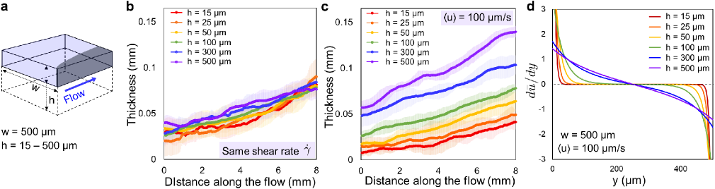
We do not directly compare this measurement with equation (22) since the channel geometries are different and the estimation of – the prefactor of equation (22) – based on the experiments done in different systems may introduce additional errors. Also, the flow structure is complicated in the wall region, and this complication is quantitatively different for channels with different dimensions. Therefore, instead, we further examine the effect of shear rate experimentally by using the channels with different heights. From the equation (25) we note that the two-dimensional wall shear rate is a function of , and the aspect ratio .
In the next set of experiments, we fix the width of the channel and vary the height and the flow speed . First, experiments were performed in channels of different heights and with the adjusted flow speeds to achieve fixed value of . For a wide range of the aspect ratio (), we obtained similar exclusion zones for a single value of . Second, experiments were performed fixing the mean flow speed while varying : we obtain the largest exclusion zone in the channel with m, and the smallest for m, which agrees with the trend predicted by the corresponding shear rates. In Lee et al.21, the excluxion zone was estimated with the scaling relation . We show in Figure 8(c) six different systems with the same values of , which demonstrate that simple estimation of the shear rate by may not provide sufficient information about the two-dimensional exclusion zone forming in channels with different dimensions. Flow structure and the channel geometry need to be fully considered.

We would like to mention more about shear flow approximation in microfluidic experiments. Figure 6(d) shows plotted versus . When the aspect ratio of the channel is large, the change in the height-averaged flow speed is mostly localized near the wall region, and for small , the change in the shear rate is less dramatic. Therefore, a typical experimental setup for testing the shear flow approximation is in the orientation where the observation is made through the small-width window () by making tall channels. In that way the experiments can assume a constant shear rate in the wall region. Knowing this, one can ask about the effect of the orientation of the channel (whether or )) on the water cleaning efficiency, under a fixed volumetric flow rate.
Similar to the height-averaged velocity , we calculated the width-averaged velocity to obtain the equivalent wall shear rate in the other orientation in the same channel (see SI section 5 for details). When and are compared (Figure S5), we obtain that the two-dimensional shear rate is always larger when the system is viewed from the narrow-side. For example, in a channel with m and m, for m/s, we obtain and . When the ion concentration gradient is created over , the measured exclusion zone is expected to be times larger than the other orientation. However, the height is 5 times larger if the ion concentration gradient is formed across , and thus the volume of particle-free water is times larger. An optimization is required for specific design and fabrication of an actual water cleaning device. Nevertheless, such shear rate criterion can be a major reference for designing the diffusiophoresis unit.
So far we have used a shear flow approximation, and, with similarity transform, we obtained a scaling estimate for the exclusion zone thickness along the flow. The relation , along with the shear rate calculation , provides useful information for predicting the trend of particle exclusion in two-dimensional configurations. In the next section, with numerical calculations we would like to investigate possible three-dimensional effects that can influence the exclusion zone measurements.
7 Three-dimensional effects and wall diffusioosmosis
Consider a three-dimensional rectangular flow (Figure 6(a)) with the flow velocity defined as equation (23). Then we can solve reaction-diffusion equations to obtain the CO2 and ion concentrations and (details in SI sections 6 and 7).
As a model case, we consider a channel flow with mm, m, and m/s, and plotted the steady-state concentration profiles of CO2 and ions in Figure 9(a,b) versus and (at ). In this configuration, it is often assumed that the concentration profiles are independent of . However, we note that due to the finite diffusivities of ions, there is a non-uniform concentration distribution of ions in the -direction (Figure 9(c)), near the upstream of the CO2 source. When the system is diffusion-dominated (Figure 9(d)), the -dependence of ion concentration is small. This result suggests that even though the main concentration gradient is established in -direction, there may be a nonzero diffusiophoretic velocity of particles generated in the height-direction, affecting the particle distribution.
The -component of nondimensional diffusiophoretic velocity is calculated numerically near the bottom wall () and plotted versus and in Figure 9(e,f). Near the inlet of the flow there are nonzero particle velocities forming in -direction to migrate particles away from the wall (). Then for this particle velocity decreases dramatically. A similar trend is observed also in the width direction; the -component of the diffusiophoretic velocity is highest near the wall where CO2 diffuses in. The nondimensional particle velocity is a measure for the particle Peclet number by definition and the calculated values suggest that the -direction particle motion is much smaller compared to the main flow speed (). Since the -direction gradient of ion concentration is generated due to the channel flow and the finite diffusivity of ions, larger will be obtained for faster flow, and for slow flow will be negligible. This means that the particle exclusion from the top and bottom walls is expected to be smaller compared to the main exclusion zone formation in the -direction in the presence of the channel flow. A study of the detailed three-dimensional particle distribution is not the main focus of the current article and so we include the contour plot of particle exclusion in the SI. The feature discussed in this section may be of consideration for maximizing the collection of clean liquid in the in-flow water cleaning systems.
One more feature to study in terms of a three-dimensional effect is the diffusioosmosis on the (top and bottom) walls. When there is a pressure-driven flow with a moderate speed, analyses that consider particle diffusiophoresis and the flow velocity may provide sufficient information about the exclusion zone formation, even though there exists diffusioosmosis forming a slip boundary condition. We consider one extreme case where the flow velocity is very small (or zero) and the exclusion zone formation is achieved by mostly (or only) the diffusion of ions. Small flow velocity decreases the overall efficiency of the water cleaning system, but if the flow is deliberately stopped periodically to achieve maximum exclusion zone thickness before each sample collection step (pulsating flow), one may ask about the influence of the wall diffusioosmosis.
We consider a model case where there is no flow along the channel and the migration of particles in the channel is driven by diffusion of ions. We can solve for the cross-sectional diffusion of ions and diffusiophoresis of particles and examine the effect of diffusioosmosis (Figure 9(g)). First, we account for diffusioosmosis along the top and bottom walls, to obtain the flow velocity () as a function of (more precisely, we use the local chemical equilibrium approximation 26, 24, and use to describe the flow velocity induced by wall diffusioosmosis; see SI section 8 for details).
In Figure 9(h), the steady-state particle distribution is plotted versus and . Due to the flow velocity induced by the wall diffusioosmosis, particle distribution is not uniform along under the concentration gradient set in the -direction. We solved for the particle distribution for the channel cross-sections with different aspect ratios and plotted the -averaged profiles versus dimensional (Figure 9(i)). For the channel with mm, the -averaged at s is plotted for different channel heights. The plots show that at smaller heights, the effect of diffusioosmosis is larger and exclude particles more. Such difference in particle exclusion may be significant in microscopic analyses of diffusiophoretic particle exclusion. However, the slight difference among different conditions would not affect practical applications, and the comparison with the no-diffusioosmosis scenario also suggests that the effect of wall diffusioosmosis can be neglected.
Throughout the paper, we showed by a theoretical model, experiments and numerical calculations that the thickness of particle exclusion zone near entrance follows the trend , where the shear rate varies with the channel dimensions. By increasing the width and height of the rectangular channel, we were able to achieve formation of larger exclusion zone. With these understandings, we would like to propose a possible two-step design for the in-flow water cleaning system (Figure 10). Again, the design suggestion is not an optimal geometry or an ultimate solution. We chose conventional microfluidic fabrication to visualize the concept in a small length scale. The ideas should be further developed and customized to a real device application.
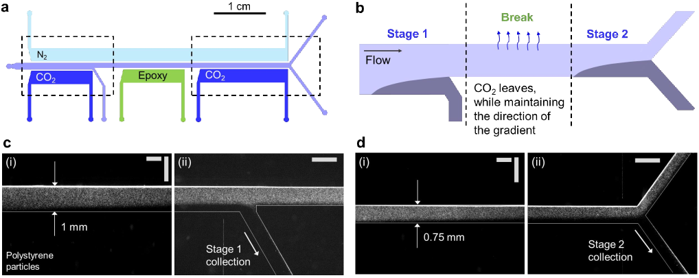
8 Toward multi-stage water cleaning
In order to visualize the idea of two-stage water cleaning, we fabricated a PDMS channel ( mm and m) that has the first bifurcation cm downstream from the inlet, and the second bifurcation cm downstream from the inlet. After the first bifurcation, the width of the remaining liquid channel is m. In order to effectively create the CO2 (or ion) concentration gradients in the second stage, we put a “break” stage where the liquid channel is in contact with the N2 channel and a channel filled with the cured optical adhesive (Norland Products; NOA 81 – Figure 10(a,b)). In the break stage, CO2 that is in the liquid phase is expected to diffuse out on the side facing the N2 channel, as the UV epoxy is impermeable to gas. While maintaining the direction of the ion concentration gradient, the absolute concentration of ions decrease at this stage25 (SI). In this way, we do not perturb the particle distribution by introducing backward ion concentration gradients. Then in the second stage, an exclusion zone is formed on the same side as the first stage, and the clean water can be collected at the final bifurcation outlet. In order to match the size of the exclusion zones with the model channel design, we adjusted the flow speed to a lower value (m/s) than our main experiments (Figure 10(c,d)).
9 Conclusion
Our study on the diffusiophoretically-generated exclusion zone is motivated by several previous studies that demonstrate diffusiophoresis in microfluidic systems. By increasing the width of the channels to mm, we observed that the exclusion zone forms in a small region near the wall facing the CO2 source. Then, with the shear flow approximation and similarity transform, we obtained a scaling law for the exclusion zone thickness (), which led to a detailed calculation for the shear rate. The wall shear rate in a rectangular channel flow is a function of , and height , so the channel geometry and the flow condition can be chosen to obtain a desired wall shear rate. With control experiments we show that the exclusion zone prediction using the shear rate is applicable to channels with various widths and heights. We also confirmed experimentally that a change in the applied CO2 pressure does not significantly vary the exclusion zone thickness in our system. Finally, we propose a design to demonstrate a continuous, multi-stage water cleaning. As the most water purification process is never a single step, by an appropriate choice of the geometrical parameters, such in-flow water cleaning system can be further scaled up to collect larger amount of cean water.
Contributions
S.S. and H.A.S. conceived the project. S.S. designed all experiments with assist of M.B., and S.S. M.B., and E.H.T. performed the experiments. S.S. and H.A.S. set up the theoretical model, and S.S. conducted numerical calculations. M.B. and E.H.T. contributed to the project through the Independent Work and Princeton Environmental Institute Summer Internship Program during their undergraduate study at Princeton University.
Conflicts of interest
S. Shim declares no conflict of interest. H. A. Stone co-founded Phoresis, Inc., which seeks to utilize CO2-driven diffusiophoresis in the water-cleaning space.
Acknowledgements
We acknowledge NSF for support via CBET-1702693. We thank Jesse T. Ault and Estella Yu for valuable discussions. M.B. and E.H.T. thank the Princeton Environmental Institute at Princeton University for supporting summer internships.
Materials and Methods
The channels are made with PDMS using standard soft lithography. All four walls are PDMS, and the bottom layer (1-mm PDMS slab) is further attached to the glass slide for microscopy (Leica DMI4000B). For all experiments using polystyrene (PS) particles (Thermo Fisher Scientific, diameter = 1 m), a dilute suspension of 0.03 vol (in DI water; Milli-Q, EMD Millipore) is used.
For the experiment with amine-modified polystyrene (a-PS) particles (Fig. 1(d); Sigma Aldrich, diameter 1 m), a dilute suspension is prepared at 5 vol in DI water. Prior to the experiment, a syringe pump was used to flow a 1 vol aqueous solution of 3-Aminopropyltriethoxysilane (APTES) through the liquid channel for 15 minutes to prevent the adhesion of amine-modified polystyrene particles to channel walls 33, 34, followed by flushing with deionized water for 15 minutes. A N2 gas stream at 1.5 psi is connected for one minute to dry the central channel.
When running the experiments, the liquid channel was first filled with the particle suspension, then N2 gas was flowed at 1.5 psi through the top channel. After one minute of observing steady-state particle flow in the liquid channel, a CO2 gas stream fixed at 10 psi is connected to the CO2 channel.
The fluorescent images are obtained every 1 second using an inverted microscope (Leica DMI4000B), with 1.25x magnification. The exclusion zone boundary was obtained by first dividing the images into 200 separate sectionst (in -direction), then detecting the mean value of the boundary position in each section. Each image piece had the width of 6 pixels, and thus the representative data point is an average of six values. The obtained values (-position of the exclusion zone boundary) are further smoothed by applying a moving average of period 20. For the time-evolution plots, a similar method is applied, where the mean value of the boundary position is obtained every six frames. No smoothing is applied for the time evolution graphs. The smooth curves in Fig. 1(e) and Fig. S1(b) are obtained using a smoothing spline fit in Matlab. The image processing and analysis are done with ImageJ and Matlab.
All equations presented in the main text are solved using a combination of Mathematica and Matlab, and the three-dimensional model included in the SI is solved with Matlab (see SI for details).
Notes and references
- 1 B. V. Derjaguin, G. Sidorenkov, E. Zubashchenko, and E. Kiseleva, Kinetic phenomena in the boundary layers of liquids 1. Capillary osmosis, Kolloidn. Zh., 1947, 9, 335-347.
- 2 B. V. Derjaguin, S. S. Dukhin, and A. A. Korotkova, Diffusiophoresis in electrolyte solutions and its role in the mechanism of film formation from rubber latexes by the method of ionic deposition, Kolloidn. Zh., 1961, 23, 53-58.
- 3 S. S. Dukhin, Z. R. Ul’berg, G. L. Dvornichenko, and B. V. Derjaguin, Diffusiophoresis in electrolyte solutions and its application to the formation of surface coatings, Russ. Chem. Bull., 1982, 31, 1535-1544.
- 4 J. L. Anderson, M. E. Lowell, and D. C. Prieve, Motion of a particle generated by chemical gradients Part 1. Non-electrolytes, J. Fluid. Mech., 1982, 117, 107-121.
- 5 D. C. Prieve, J. L. Anderson, J. P. Ebel, and M. E. Lowell, Motion of a particle generated by chemical gradients. Part 2. Electrolytes, J. Fluid. Mech., 1984, 148, 247-269.
- 6 D. C. Prieve, Migration of a colloidal particle in a gradient of electrolyte concentration, Adv. Colloid Interface Sci., 1982, 16, 321-335.
- 7 D. C. Prieve, and R. Roman, Diffusiophoresis of a rigid sphere through a viscous electrolyte solution, J. Chem. Soc. Faraday Trans. 2, 1987, 83(3), 1287-1306.
- 8 B. Abécassis, C. Cottin-Bizonne, C. Ybert, A. Ajdari, and L. Bocquet, Nat. Mater., 2008, 7, 785-789.
- 9 J. J. McDermott, A. Kar, M. Daher, S. Klara, G. Wang, A. Sen, and D. Velegol, Langmuir, 2012, 28, 15491-15497.
- 10 D. Florea, S. Musa, J. M. R. Huyghe, and H. M. Wyss, Long-range repulsion of colloids driven by ion exchange and diffusiophoresis, Proc. Natl. Acad. Sci. U.S.A., 2014, 111(18), 6554-6559.
- 11 J. Palacci, C. Cottin-Bizonne, C. Ybert, and L. Bocquet, Osmotic traps for colloids and macromolecules based on logarithmic sensing in salt taxis, Soft Matter, 2012, 8, 980-994.
- 12 A. Kar, T.-Y. Chiang, I. O. Rivera, A. Sen, and D. Velegol, Enhanced transport into and out of dead-end pores, ACS Nano, 2015, 9, 746-753.
- 13 S. Shin, E. Um, B. Sabass, J. T. Ault, M. Rahimi, P. B. Warren, and H. A. Stone, Size-dependent control of colloid transport via solute gradients in dead-end channels, Proc. Natl. Acad. Sci., 2016, 113, 257-261.
- 14 S. Battat, J. T. Ault, S. Shin, S. Khodaparast, and H. A. Stone, Particle entrainment in dead-end pores by diffusiophoresis, Soft Matter, 2019, 15, 3879-3885.
- 15 N. Shi, R. Nery-Azevedo, A. I. Abdel-Fattah, and T. M. Squires, Diffusiophoretic focusing of suspended colloids, Phys. Rev. Lett., 2016, 117, 258001.
- 16 J. T. Ault, P. B. Warren, S. Shin, and H. A. Stone, Diffusiophoresis in one-dimensional solute gradients, Soft Matter, 2017, 13, 9015-9023.
- 17 A. Gupta, B. Rallabandi, and H. A. Stone, Diffusiophoretic and diffusioosmotic velocities for mixtures of valence-asymmetric electrolytes, Phys. Rev. Fluids, 2019, 4, 043702.
- 18 J. L. Wilson, S. Shim, Y. E. Yu, A. Gupta, and H. A. Stone, Diffusiophoresis in multivalent electrolytes, Langmuir, 2020, 36, 7014-7020.
- 19 A. Gupta, S. Shim, and H. A. Stone, Diffusiophoresis: from dilute to concentrated electrolytes, Soft Matter, 2020, 16, 6975-6984.
- 20 J. S. Paustian, C. D. Angulo, R. Nery-Azevedo, N. Shi, A. I. Abdel-Fattah, and T. M. Squires, Direct measurements of colloidal solvophoresis under imposed solvent and solute gradients, Langmuir, 2015, 31, 4402-4410.
- 21 H. Lee, J. Kim, J. Yang, S. W. Seo, and S. J. Kim, Diffusiophoretic exclusion of colloidal particles for continuous water purification. Lab Chip, 2018, 18, 1713.
- 22 S. Shin, O. Shardt, P. B. Warren, and H. A. Stone, Membraneless water filtration using CO2, Nature Comm., 2017, 8, 15181.
- 23 S. Shim, Interfacial Flows with Heat and Mass Transfer. PhD Thesis, 2017, Princeton University.
- 24 O. Shardt, B. Rallabandi, S. Shim, S. Shin, P. B. Warren, and H. A. Stone, Driving diffusiophoresis by the dissolution of gas, Under review.
- 25 S. Shim and H. A. Stone, CO2-leakage-driven diffusiophoresis causes spontaneous accumulation of charged materials in channel flow, Proc. Natl. Acad. Sci. U.S.A., 2020, 117(42), 25985-25990.
- 26 S. Shim, S. Khodaparast, C.-Y. Lai, J. Yan, J. T. Ault, B. Rallabandi, O. Shardt, and H. A. Stone, CO2-driven diffusiophoresis for maintaining a bacteria-free surface. Soft Matter, 2021, 17, 2568-2576.
- 27 T. J. Shimokusu, V. G. Maybruck, J. T. Ault, and S. Shin, Colloid separation by CO2-induced diffusiophoresis. Langmuir, 2020, 36, 7032-7038.
- 28 M. Seo, S. Park, D. Lee, H. Lee, and S. J. Kim, Continuous and spontaneous nanoparticle separation by diffusiophoresis, Lab Chip, 2020, 20, 4118-4127.
- 29 C. L. Yaws, Handbook of Properties for Environmental and Green Engineering, Gulf Publishing Company, 2008, 1st edn.
- 30 W. M. Haynes, CRC Handbood of Chemistry and Physics CRC Press, 2015, 96th edn.
- 31 W. L. Jolly, Modern Inorganic Chemistry McGraw-Hill, New york, 1991, 2nd edn.
- 32 W. D. Ristenpart and H. A. Stone, Michaelis-Menten kinetics in shear flow: Similarity solutions for multi-step reactions, Biomicrofluidics, 2012, 6, 014108.
- 33 Lee, N.Y. and Chung, B.H. Novel Poly(dimethylsiloxane) bonding strategy via room temperature “chemical gluing." Langmuir, 25, 3861–3866 (2009)
- 34 Zhou, J., Ellis, A.V. and Voelcker, N.H. Recent developments in PDMS surface modification for microfluidic devices. Electrophoresis 31, 2–16 (2010)