Sharp scattering threshold for the cubic-quintic NLS in the focusing-focusing regime

Abstract

We consider the large data scattering problem for the 2D and 3D cubic-quintic nonlinear Schrödinger equation in the focusing-focusing regime. Our attention is firstly restricted to the 2D space, where the cubic nonlinearity is $L^{2}$-critical. We establish a new type of scattering criterion that is uniquely determined by the mass of the initial data, which differs from the classical setting based on the Lyapunov functional. At the end, we formulate a solely mass-determining scattering threshold for the 3D cubic-quintic nonlinear Schrödinger equation in the focusing-focusing regime.

1 Introduction and main results

In this paper, we consider the cubic-quintic nonlinear Schrödinger equation

$$i\partial_{t}u+\Delta u+\mu_{1}|u|^{2}u+\mu_{2}|u|^{4}u=0\quad\text{in $\mathbb{R}\times\mathbb{R}^{d}$}$$ (1.1)

for $d=2,3$. The cubic-quintic nonlinear Schrödinger equation (CQNLS) serves as a toy model in many physical applications such as nonlinear optics and Bose-Einstein condensation. Physically, the cubic and quintic nonlinearities model the two-body and three-body interactions respectively. The signs $\mu_{i}$ can be tuned to be defocusing ($\mu_{i}<0$) or focusing ($\mu_{i}>0$), indicating the repulsivity or attractivity of the many-body interactions. We refer to [17, 21, 36] and the references therein for a comprehensive introduction on the physical background of the CQNLS.

On the other hand, the CQNLS has also attracted much attention from the mathematical community due to its abundant analytical structure: one easily verifies the $L^{2}$-criticality of the quintic term in 1D, the $L^{2}$-criticality of the cubic term in 2D and the $\dot{H}^{1}$-criticality of the quintic term in 3D. Additionally, the mixed type nature of the CQNLS prevents any possible application of scaling invariance property, which makes the mathematical analysis more subtle and challenging. For recent mathematical progress on the study of the CQNLS with a particular focus on the scattering and blow-up phenomenon, we refer to [37, 16, 27, 15, 12, 33, 26, 11].

Our particular interest is firstly devoted to establishing a sharp scattering threshold for the 2D CQNLS in the focusing-focusing regime ($\mu_{1},\mu_{2}>0$), which has not been considered in any of the above mentioned references. In particular, we see no possibility to easily adapt the existing arguments to the focusing-focusing model; To achieve our aim, we need some new ideas and ingredients. For simplicity, we set $\mu_{1}=\mu_{2}=1$ and in the following we consider the normalized CQNLS

$$i\partial_{t}u+\Delta u+|u|^{2}u+|u|^{4}u=0\quad\text{in $\mathbb{R}\times\mathbb{R}^{2}$}.$$ (1.2)

In [37], it was shown that as long as $\mu_{1},\mu_{2}<0$ (namely both nonlinearities are defocusing), (1.1) is globally well-posed and scatters in time for any initial data $u(0)=u_{0}\in H^{1}(\mathbb{R}^{2})$. The proof relies on the so-called interaction Morawetz inequalities and the defocusing nature of the model is essential, hence the proof can not be adapted to other types of models. In fact, the result from [37] does not hold when at least one of the $\mu_{i}$ is positive: (1.1) might possess solutions that blow-up in finite time, or soliton solutions. Here, the soliton solutions are referred to solutions $u$ of (1.1) having the form $u(t,x)=e^{i\omega t}S(x)$ with $\omega\in\mathbb{R}$, where $S$ satisfies the stationary CQNLS

$$-\Delta S+\omega S-\mu_{1}|S|^{2}S-\mu_{2}|S|^{4}S=0\quad\text{in $\mathbb{R}^{2}$}.$$ (1.3)

For the normalized focusing-focusing model, (1.3) reads

$$-\Delta S+\omega S-|S|^{2}S-|S|^{4}S=0\quad\text{in $\mathbb{R}^{2}$}.$$ (1.4)

It turns out that the energy level corresponding to soliton solutions is the minimal threshold for a solution being failed to meet the dichotomy of scattering and blow-up. Our starting point is the result in [34] given by Soave, where the author studied the existence problem of solutions of (1.4). Therein, Soave considered the following variational problem

$$m_{c}=\inf_{u\in H^{1}(\mathbb{R}^{2})}\{\mathcal{H}(u):\mathcal{M}(u)=c,\mathcal{K}(u)=0\}$$ (1.5)

for $c>0$, where

$$\mathcal{M}(u) :=\|u\|^{2}_{2},$$

$$\mathcal{H}(u) :={\frac{1}{2}}\|\nabla u\|_{2}^{2}-{\frac{1}{4}}\|u\|^{{4}}_{{4}}-{\frac{1}{6}}\|u\|^{{6}}_{{6}},$$

$$\mathcal{K}(u) :=\|\nabla u\|_{2}^{2}-{\frac{1}{2}}\|u\|_{4}^{4}-\frac{2}{3}\|u\|_{6}^{6}.$$

Physically, $\mathcal{M}(u),\mathcal{H}(u),\mathcal{K}(u)$ denote the mass, energy and virial respectively. It was shown in [34] that $\mathcal{K}(u)=0$ is a natural constraint, thus using the Lagrange multiplier theorem we know that any optimizer of (1.5) is automatically a solution of (1.4). An optimizer of $m_{c}$ is also said to be a ground state since it has the least energy among all candidates. To formulate the result in [34], we also denote by $Q$ the unique positive and radially symmetric solution of

$$-\Delta Q+Q-Q^{3}=0.$$

Having all the preliminaries we are able to introduce the following result from [34]:

Theorem 1.1 ([34]).

We have the following existence and blow-up results:

• Existence of ground state: For any $c\in(0,{\mathcal{M}(Q)})$ the variational problem (1.5) has a minimizer $S_{c}$ with $\mathcal{H}(S_{c})=m_{c}\in(0,\infty)$. Moreover, $S_{c}$ is a solution of (1.4) with some $\omega>0$. In addition, $S_{c}$ can be chosen to be positive and radially symmetric.

• Blow-up criterion: Assume that $u_{0}\in H^{1}(\mathbb{R}^{2})$ satisfies the conditions $\mathcal{M}(u_{0})\in(0,{\mathcal{M}(Q)})$, $\mathcal{H}(u_{0})<m_{\mathcal{M}(u_{0})}$ and $\mathcal{K}(u_{0})<0$. Assume also that $|x|u_{0}\in L^{2}(\mathbb{R}^{2})$. Then the solution $u$ of (1.2) with $u(0)=u_{0}$ blows-up in finite time.

The aim of the present paper is to show that the threshold given by Soave is exactly the sharp scattering threshold for (1.2).

Theorem 1.2.

Define the set

$$\mathcal{A} :=\{u\in H^{1}(\mathbb{R}^{2}):\mathcal{M}(u)<{\mathcal{M}(Q)},\mathcal{H}(u)<m_{\mathcal{M}(u)},\mathcal{K}(u)>0\}$$ (1.6)

and assume that $u_{0}\in\mathcal{A}$. Then the solution $u$ of (1.2) with $u(0)=u_{0}$ is global and scatters in time.

We should compare the scattering criterion (1.6) with the one given in [2], which is nowadays the golden rule for large data scattering problems of NLS with combined power type nonlinearities. Therein, the authors considered the NLS

$$i\partial_{t}u+\Delta u+|u|^{p-2}u+|u|^{\frac{4}{d-2}}u=0\quad\text{in $\mathbb{R}\times\mathbb{R}^{d}$}$$ (1.7)

for $d\geq 5$ and $p\in(2+\frac{4}{d},2+\frac{4}{d-2})$, namely the focusing energy-critical NLS with a focusing mass-supercritical and energy-subcritical perturbation. To formulate the scattering threshold, the authors imposed the so-called Lyapunov functional

$$\mathcal{S}_{\omega}(u):=\frac{\omega}{2}\mathcal{M}(u)^{2}+\mathcal{H}(u)$$ (1.8)

and considered the variational problem

$$\gamma_{\omega}:=\inf_{u\in H^{1}(\mathbb{R}^{2})\setminus\{0\}}\{\mathcal{S}_{\omega}(u):\mathcal{K}(u)=0\}.$$ (1.9)

The following result is due to [1, 2, 3]:

Theorem 1.3 ([1, 2, 3]).

Let $d\geq 3$ and $\omega>0$. Then

• For any $d\geq 3$ and $\omega>0$ we have $\gamma_{\omega}\in(0,\frac{\mathcal{S}^{\frac{d}{2}}}{d}]$, where $\mathcal{S}$ is the optimal constant for the Sobolev inequality.

• For any $d\geq 4$ and $\omega>0$ and for $d=3$ and any sufficiently small $\omega>0$ we have $\gamma_{\omega}\in(0,\frac{\mathcal{S}^{\frac{d}{2}}}{d})$. Moreover, the variational problem (1.9) possesses an optimizer $P_{\omega}$. Consequently, the optimizer $P_{\omega}$ is a soliton solution of (1.7) with the given $\omega$.

• Assume that

  $$u_{0}\in\{v\in H^{1}(\mathbb{R}^{d}):\mathcal{S}_{\omega}(v)<\gamma_{\omega},\mathcal{K}(v)>0\}.$$ (1.10)

  Additionally we assume that $u_{0}$ is radially symmetric when $d=3$. Then the solution $u$ of (1.7) with $u(0)=u_{0}$ is global and scatters in time.

We should point out that the scattering results given in [2] were originally formulated in the cases $d\geq 5$. The results can nonetheless be extended to all dimensions $d\geq 3$ in a natural way by combining with the results from [24] and the recent published paper [19]. The scattering criterion (1.10) has been later successfully applied in [30, 40, 31, 32, 16, 41] to formulate a sharp scattering threshold for NLS with combined power type nonlinearities in different regimes. However, (1.10) seems not to be compatible with problems having focusing $L^{2}$-critical nonlinearity due to the following reason: The constraint $\mathcal{M}(u)<\mathcal{M}(Q)$ is essential since the $L^{2}$-critical nonlinearity $|u|^{\frac{4}{d}}u$ shares the same scaling of the Laplacian $\Delta u$ under the scaling operator

$$T_{\lambda}u(x):=\lambda^{\frac{d}{2}}u(\lambda x).$$

However, by considering the Lyapunov functional $\mathcal{S}_{\omega}$ we would have double constraints on the mass of the initial data, which might violate the conciseness of the scattering threshold. By comparison with (1.10) we also see that the scattering criterion (1.6) has the advantage that it is uniquely determined by the mass of the initial data. Such a solely mass-determining threshold could also be more physically relevant in the following sense: besides being a conserved quantity, the mass also measures many physically important quantities such as the power supply in nonlinear optics, or the total number of particles in the Bose-Einstein condensation.

As a surprising byproduct, we are able to formulate a scattering criterion for the problem (1.7) within the framework of the present paper by also invoking the results from [35, 38]. In particular, there is no smallness condition and mass constraint in all dimensions and the energy threshold is exactly the ground state energy which is positive and smaller than $d^{-1}\mathcal{S}^{\frac{d}{2}}$. We will continue the discussion in Section 6. As a consequence of Theorem 6.2 given below, we are able to impose the following solely mass-determining scattering threshold for the 3D CQNLS in the focusing-focusing regime:

Theorem 1.4.

Let $d=3$ and $\mu_{1}=\mu_{2}=1$. Define the set

$$\mathcal{B} :=\{u\in H^{1}(\mathbb{R}^{3}):\mathcal{H}(u)<m_{\mathcal{M}(u)},\mathcal{K}(u)>0\}$$ (1.11)

(where $\mathcal{K}(u)$ is suitably redefined in the 3D case) and assume that $u_{0}\in\mathcal{B}\cap H^{1}_{\mathrm{rad}}(\mathbb{R}^{3})$. Then the solution $u$ of (1.1) with $u(0)=u_{0}$ is global and scatters in time.

Remark 1.5.

We note that unlike the 2D case, in Theorem 1.4 there is no mass constraint imposed for the initial data. This difference stems from the fact that the cubic nonlinearity is mass-critical and mass-supercritical in 2D and 3D respectively. To be more precise, when applying the $L^{2}$-scaling $u\mapsto T_{\lambda}u$ to the quantity $\frac{1}{2}\|\nabla u\|_{2}^{2}-\frac{1}{4}\|u\|_{4}^{4}$ in 2D, we see that

$$\frac{1}{2}\|\nabla(T_{\lambda}u)\|_{2}^{2}-\frac{1}{4}\|T_{\lambda}u\|_{4}^{4}=\lambda^{2}\Big{(}\frac{1}{2}\|\nabla u\|_{2}^{2}-\frac{1}{4}\|u\|_{4}^{4}\Big{)}.$$

Therefore, the quantity $\frac{1}{2}\|\nabla u\|_{2}^{2}-\frac{1}{4}\|u\|_{4}^{4}$ does not vary w.r.t. scaling and keeping the mass below the (mass-critical) ground state is essential for applications of Gagliardo-Nirenberg inequalities. Such heuristics do not hold any longer in the 3D case. Indeed, by applying the $L^{2}$-scaling to the quantity $\frac{1}{2}\|\nabla u\|_{2}^{2}-\frac{1}{4}\|u\|_{4}^{4}$ in 3D we obtain

$$\frac{1}{2}\|\nabla(T_{\lambda}u)\|_{2}^{2}-\frac{1}{4}\|T_{\lambda}u\|_{4}^{4}=\frac{\lambda^{2}}{2}\|\nabla u\|_{2}^{2}-\frac{\lambda^{3}}{4}\|u\|_{4}^{4}.$$

We see in this case that the quantity $\frac{1}{2}\|\nabla u\|_{2}^{2}-\frac{1}{4}\|u\|_{4}^{4}$ does not play the same role as in 2D and the mass constraint is no longer relevant. Rather, we should consider the function $\lambda\mapsto\frac{\lambda^{2}}{2}\|\nabla u\|_{2}^{2}-\frac{\lambda^{3}}{4}\|u\|_{4}^{4}$ and the corresponding variational analysis becomes more delicate in comparison with the 2D case. We refer to the papers [34, 35, 38] for a more detailed survey on such phenomenon. ∎

The study on the existence and stability results of (1.3) is also a very interesting topic. In this direction, we refer to the classical papers [7, 8, 39, 14, 22, 9] and also the recent papers [5, 34, 35, 38].

Roadmap for the proof of Theorem 1.2

We summarize here briefly the idea for the proof of Theorem 1.2. The proof follows the classical concentration compactness arguments given by Kenig and Merle [24]: by assuming that the claim in Theorem 1.2 does not hold, we are able to derive a minimal blow-up solution $u_{c}$ of (1.2) with

$$\|\langle\nabla\rangle^{\frac{1}{2}}u_{c}\|_{L_{t,x}^{4}(\mathbb{R})}=\infty,$$

which also satisfies $u_{c}=0$ and thus leads to a contradiction. The main challenge arises from the fact that since the scattering is considered w.r.t. the $H^{1}$-topology, it is impossible to prove Theorem 1.2 only relying on the energy $\mathcal{H}$. It is at this point to note that the $H^{1}$-norm of a solution $u$ of (1.2) can be controlled by the Lyapunov functional $\mathcal{S}_{\omega}(u)$, which is not the case here. To build up the inductive contradiction hypothesis, we should rather take the mass and energy of the initial data into account simultaneously. To be more precise, we utilize the mass-energy-indicator functional (MEI-functional) $\mathcal{D}$ introduced in [27] to derive a minimal blow-up solution. The idea can be described as follows: a mass-energy pair $(\mathcal{M}(u),\mathcal{H}(u))$ being admissible implies $\mathcal{D}(u)\in(0,\infty)$; In order to escape the admissible region $\Omega$, a function $u$ must approach the boundary of $\Omega$ and one would deduce $\mathcal{D}(u)\to\infty$. We can therefore assume that the supremum $\mathcal{D}^{*}$ of $\mathcal{D}(u)$ running over all admissible $u$ is finite, which leads to a contradiction and we conclude that $\mathcal{D}^{*}=\infty$, which will finish the desired proof. However, the situation by the focusing-focusing model is more delicate: a mass-energy pair being admissible does not automatically imply the positivity of the virial $\mathcal{K}$. In particular, it is not trivial that the linear profiles would have positive virial at the first glance. We will appeal to the geometric properties of the MEI-functional $\mathcal{D}$, combining with the variational arguments from [2], to overcome this difficulty.

Outline of the paper

In Section 2 we collect some auxiliary tools from [15, 33] that will be useful by the construction of the minimal blow-up solution; Section 3 is devoted to the variational estimates and the construction of the MEI-functional $\mathcal{D}$; Finally, we prove in Section 4 and Section 5 the existence and extinction of the minimal blow-up solution respectively. In Section 6 we formulate a scattering criterion for the problem (1.7) under the framework of the present paper. In A we establish the precise endpoint values $m_{0}$ and $m_{Q}$ of the curve $c\mapsto m_{c}$ in 2D.

1.1 Notation and definitions

We use the notation $A\lesssim B$ whenever there exists some positive constant $C$ such that $A\leq CB$. Similarly we define $A\gtrsim B$ and use $A\sim B$ when $A\lesssim B\lesssim A$. We denote by $\|\cdot\|_{p}$ the $L^{p}(\mathbb{R}^{d})$-norm for $p\in[1,\infty]$. We similarly define the $H^{1}(\mathbb{R}^{d})$-norm by $\|\cdot\|_{H^{1}}$. The following quantities will be used throughout the paper:

$$\mathcal{M}(u) :=\|u\|^{2}_{2},$$

$$\mathcal{H}(u) :={\frac{1}{2}}\|\nabla u\|_{2}^{2}-{\frac{1}{4}}\|u\|^{{4}}_{{4}}-{\frac{1}{6}}\|u\|^{{6}}_{{6}},$$

$$\mathcal{K}(u) :=\|\nabla u\|_{2}^{2}-{\frac{1}{2}}\|u\|_{4}^{4}-\frac{2}{3}\|u\|_{6}^{6},$$

$$\mathcal{I}(u) :=\mathcal{H}(u)-\frac{1}{2}\mathcal{K}(u)=\frac{1}{6}\|u\|_{6}^{6}.$$

We will also frequently use the scaling operator

$$T_{\lambda}u(x) :=\lambda^{\frac{d}{2}}u(\lambda x).$$

One easily verifies that the $L^{2}$-norm is invariant under this scaling. We denote by $Q$ the unique positive and radially symmetric ground state of

$$-\Delta Q+Q-Q^{3}=0.$$

For the existence and uniqueness of $Q$, we refer to [39] and [28] respectively. We denote by $\mathrm{C}_{\mathrm{GN}}$ the 2D optimal $L^{2}$-critical Gagliardo-Nirenberg constant, i.e.

$$\mathrm{C}_{\mathrm{GN}}=\inf_{u\in H^{1}(\mathbb{R}^{2})\setminus\{0\}}\frac{\|\nabla u\|_{2}^{2}\|u\|_{2}^{2}}{\|u\|_{{4}}^{{4}}}.$$ (1.12)

Using Pohozaev identities (see for instance [7]) and scaling arguments one easily verifies that

$$\mathrm{C}_{\mathrm{GN}}=\frac{1}{2}\mathcal{M}(Q).$$ (1.13)

We also denote by $\widehat{\mathrm{C}}_{\mathrm{GN}}$ the optimal Gagliardo-Nirenberg constant for the quintic nonlinearity, i.e.

$$\widehat{\mathrm{C}}_{\mathrm{GN}}=\inf_{u\in H^{1}(\mathbb{R}^{2})\setminus\{0\}}\frac{\|\nabla u\|_{2}^{4}\|u\|_{2}^{2}}{\|u\|_{{6}}^{{6}}}.$$ (1.14)

For $d\geq 3$ we denote by $\mathcal{S}$ the optimal constant of the Sobolev inequality, i.e.

$$\mathcal{S}:=\inf_{u\in\mathcal{D}^{1,2}(\mathbb{R}^{d})\setminus\{0\}}\frac{\|\nabla u\|_{2}^{2}}{\|u\|_{2^{*}}^{2}}.$$

Here, the space $\mathcal{D}^{1,2}(\mathbb{R}^{d})$ is defined by

$$\mathcal{D}^{1,2}(\mathbb{R}^{d}):=\{u\in L^{2^{*}}(\mathbb{R}^{d}):\nabla u\in L^{2}(\mathbb{R}^{d})\}$$

and $2^{*}=\frac{2d}{d-2}$. For an interval $I\subset\mathbb{R}$, the space $L_{t}^{q}L_{x}^{r}(I)$ is defined by

$$L_{t}^{q}L_{x}^{r}(I):=\{u:I\times\mathbb{R}^{2}\to\mathbb{C}:\|u\|_{L_{t}^{q}L_{x}^{r}(I)}<\infty\},$$

where

$$\|u\|^{q}_{L_{t}^{q}L_{x}^{r}(I)}:=\int_{\mathbb{R}}\|u\|^{q}_{r}\,dt.$$

A pair $(q,r)$ is said to be $L^{2}$-admissible in 2D if $q,r\in[2,\infty]$, $\frac{2}{q}+\frac{2}{r}=1$ and $(q,r)\neq(2,\infty)$. For any $L^{2}$-admissible pairs $(q_{1},r_{1})$ and $(q_{2},r_{2})$ we have the following Strichartz estimates: if $u$ is a solution of

$$i\partial_{t}u+\Delta u=F(u)$$ (1.15)

in $I\subset\mathbb{R}$ with $t_{0}\in I$ and $u(t_{0})=u_{0}$, then

$$\|u\|_{L_{t}^{q}L_{x}^{r}(I)}\lesssim\|u_{0}\|_{2}+\|F(u)\|_{L_{t}^{q_{2}^{\prime}}L_{x}^{r_{2}^{\prime}}(I)},$$ (1.16)

where $(q_{2}^{\prime},r_{2}^{\prime})$ is the Hölder conjugate of $(q_{2},r_{2})$. For a proof, we refer to [23, 13]. The $S$-norm is defined by

$$\|u\|_{S(I)}:=\sup_{q\in(2^{+},\infty]}\|u\|_{L_{t}^{q}L_{x}^{r}(I)},$$ (1.17)

where the supremum is taken over all $L^{2}$-admissible pairs $(q,r)$ with $q\in(2^{+},\infty]$ and $2^{+}>2$ is some positive constant that is sufficiently close to $2$. In this paper, the scattering concept is referred to the following definition:

Definiton 1.6 (Scattering).

A global solution $u$ of (1.2) is said to be forward in time scattering if there exists some $\phi_{+}\in H^{1}(\mathbb{R}^{2})$ such that

$$\lim_{t\to\infty}\|u(t)-e^{it\Delta}\phi_{+}\|_{H^{1}}=0.$$ (1.18)

A backward in time scattering solution is similarly defined. $u$ is then called a scattering solution when it is both forward and backward in time scattering.

We define the Fourier transform of a function $f$ by

$$\hat{f}(\xi)=\mathcal{F}(f)(\xi)=\int_{\mathbb{R}^{2}}f(x)e^{-i\xi\cdot x}\,dx.$$

For $s\in\mathbb{R}$, the multipliers $|\nabla|^{s}$ and $\langle\nabla\rangle^{s}$ are defined by the symbols

$$|\nabla|^{s}f(x) =\mathcal{F}^{-1}\Big{(}|\xi|^{s}\hat{f}(\xi)\Big{)}(x),$$

$$\langle\nabla\rangle^{s}f(x) =\mathcal{F}^{-1}\Big{(}(1+|\xi|^{2})^{\frac{s}{2}}\hat{f}(\xi)\Big{)}(x).$$

Let $\psi\in C^{\infty}_{c}(\mathbb{R}^{2})$ be a fixed radial, non-negative function such that $\psi(x)=1$ if $|x|\leq 1$ and $\psi(x)=0$ for $|x|\geq\frac{11}{10}$. Then for $N>0$, we define the Littlewood-Paley projectors by

$$P_{\leq N}f(x) =\mathcal{F}^{-1}\Big{(}\psi\Big{(}\frac{\xi}{N}\Big{)}\hat{f}(\xi)\Big{)}(x),$$

$$P_{N}f(x) =\mathcal{F}^{-1}\Big{(}\Big{(}\psi\Big{(}\frac{\xi}{N}\Big{)}-\psi\Big{(}\frac{2\xi}{N}\Big{)}\Big{)}\hat{f}(\xi)\Big{)}(x),$$

$$P_{\geq N}f(x) =\mathcal{F}^{-1}\Big{(}\Big{(}1-\psi\Big{(}\frac{\xi}{N}\Big{)}\Big{)}\hat{f}(\xi)\Big{)}(x).$$

2 Auxiliary preliminaries

In this section we collect some useful auxiliary lemmas from [15, 33]. The proofs will be omitted here and we refer to [15, 33] for further details. We begin with the small data well-posedness and stability theory, which can be proved in a standard way.

Lemma 2.1 (Small data well-posedness).

For any $A>0$ there exists some $\beta>0$ such that the following is true: Suppose that $I$ is some interval and $t_{0}\in I$. Suppose also that $u_{0}\in H^{1}(\mathbb{R}^{2})$ with

$$\|u_{0}\|_{H^{1}}\leq A$$ (2.1)

and

$$\|\langle\nabla\rangle e^{i(t-t_{0})\Delta}u_{0}\|_{{L_{t,x}^{4}}(I)}\leq\beta.$$ (2.2)

Then (1.2) has a unique solution $u\in C(I;H^{1}(\mathbb{R}^{2}))$ with $u(t_{0})=u_{0}$ such that

$$\|\langle\nabla\rangle u\|_{S(I)} \lesssim\|u_{0}\|_{H^{1}},$$ (2.3)

$$\|\langle\nabla\rangle u\|_{{L_{t,x}^{4}}(I)} \leq 2\|\langle\nabla\rangle e^{i(t-t_{0})\Delta}u_{0}\|_{{L_{t,x}^{4}}(I)}.$$ (2.4)

Denote by $I_{\max}$ the maximal lifespan of $u$. We then have the following blow-up and scattering criterion: if the solution $u$ of (1.2) satisfies

$$\|\langle\nabla\rangle^{\frac{1}{2}}u\|_{{L_{t,x}^{4}}(I_{\max})}<\infty,$$ (2.5)

then $I_{\max}=\mathbb{R}$ and $u$ scatters in both positive and negative time.

Remark 2.2.

Using Strichartz we infer that

$$\|\langle\nabla\rangle e^{i(t-t_{0})\Delta}u_{0}\|_{{L_{t,x}^{4}}(I)}\lesssim\|u_{0}\|_{H^{1}}.$$ (2.6)

Thus Lemma 2.1 is applicable for all $u_{0}$ with sufficiently small $H^{1}$-norm. ∎

Lemma 2.3 (Stability).

Let $u\in C(I;H^{1}(\mathbb{R}^{2}))$ be a solution of (1.2) defined on some interval $I\ni t_{0}$. Assume also that $w$ is an approximate solution of the following perturbed NLS

$$i\partial_{t}w+\Delta w=-|w|^{2}w-|w|^{4}w+e$$ (2.7)

such that

$$\|w\|_{L_{t}^{\infty}H_{x}^{1}(I)} \leq B_{1},$$ (2.8)

$$\|\langle\nabla\rangle^{\frac{1}{2}}(u(t_{0})-w(t_{0}))\|_{2} \leq B_{2},$$ (2.9)

$$\|\langle\nabla\rangle^{\frac{1}{2}}w\|_{{L_{t,x}^{4}}(I)} \leq B_{3}$$ (2.10)

for some $B_{1},B_{2},B_{3}>0$. Then there exists some positive $\beta_{0}=\beta_{0}(B_{1},B_{2},B_{3})\ll 1$ with the following property: if

$$\|\langle\nabla\rangle^{\frac{1}{2}}e^{i(t-t_{0})\Delta}(u(t_{0})-w(t_{0}))\|_{{L_{t,x}^{4}}(I)} \leq\beta,$$ (2.11)

$$\|\langle\nabla\rangle^{\frac{1}{2}}e\|_{L_{t,x}^{\frac{4}{3}}(I)} \leq\beta$$ (2.12)

for some $0<\beta<\beta_{0}$, then

$$\|\langle\nabla\rangle^{\frac{1}{2}}(u-w)\|_{{L_{t,x}^{4}}(I)} \leq C(B_{1},B_{2},B_{3})\beta,$$ (2.13)

$$\|\langle\nabla\rangle^{\frac{1}{2}}(u-w)\|_{S(I)} \leq C(B_{1},B_{2},B_{3}),$$ (2.14)

$$\|\langle\nabla\rangle^{\frac{1}{2}}u\|_{S(I)} \leq C(B_{1},B_{2},B_{3}).$$ (2.15)

Next we introduce the linear profile decomposition used in present paper. Since (1.2) is a focusing mass-critical NLS with a mass-supercritical and energy-subcritical perturbation, we should apply an $L^{2}$-profile decomposition on the approximating sequence $(\psi_{n})_{n}$ rather than an $\dot{H}^{1}$-profile decomposition as in [25]. The classical $L^{2}$-profile decomposition was originally given by [10, 29, 4] and later applied in [16] for the radial mass-energy double critical NLS. To remove the radial restriction we should appeal to the following linear profile decomposition from [15]:

Lemma 2.4 (Linear profile decomposition).

Let $(\psi_{n})_{n}$ be a bounded sequence in $H^{1}(\mathbb{R}^{2})$. Then up to a subsequence of $(\psi_{n})_{n}$, there exist some number $K^{*}\in\mathbb{N}\cup\{\infty\}$, a sequence of nonzero linear profiles $(\phi^{j})_{1\leq j\leq K^{*}}\subset L^{2}(\mathbb{R}^{2})$, a sequence of symmetry parameters $(\lambda_{n}^{j},t_{n}^{j},x_{n}^{j},\xi_{n}^{j})_{n\in\mathbb{N},1\leq j\leq K^{*}}\subset(0,\infty)\times\mathbb{R}\times\mathbb{R}^{2}\times\mathbb{R}^{2}$ with $\sup_{n\in\mathbb{N}}|\xi_{n}^{j}|\lesssim_{j}1$ and a sequence of remainders $(w_{n}^{k})_{n\in\mathbb{N},1\leq k\leq K^{*}}\subset H^{1}(\mathbb{R}^{2})$ such that

• The parameters $(\lambda_{n}^{j},t_{n}^{j},x_{n}^{j},\xi_{n}^{j})_{n,j}$ satisfy

  $$\lim_{n\to\infty} \Big{\{}\Big{|}\log\frac{\lambda_{n}^{j}}{\lambda_{n}^{l}}\Big{|}+\frac{|t_{n}^{j}-t_{n}^{l}|}{(\lambda_{n}^{j})^{2}}$$

  $$\quad\quad\quad+\lambda_{n}^{j}|\xi_{n}^{j}-\xi_{n}^{l}|+\frac{|x_{n}^{j}-x_{n}^{l}+2t_{n}^{j}(\xi_{n}^{j}-\xi_{n}^{l})|}{\lambda_{n}^{j}}\Big{\}}=\infty$$ (2.16)

  for all finite $1\leq j,l\leq K^{*}$ with $j\neq l$. Moreover,

  $$\lim_{n\to\infty}\lambda_{n}^{j} =\lambda^{j}_{\infty}\in\{1,\infty\},$$ (2.17)

  $$\lambda_{n}^{j} \equiv 1\quad\text{if $\lambda_{\infty}^{j}=1$}.$$ (2.18)

• There exists some $\theta\in(0,1)$ such that for any finite $1\leq k\leq K^{*}$ we have the decomposition

  $$\psi_{n}=\sum_{j=1}^{k}T_{n}^{j}P_{n}^{j}\phi^{j}+w_{n}^{k},$$ (2.19)

  where

  $$T_{n}^{j}u(x):=e^{ix\cdot\xi_{n}^{j}}e^{-it_{n}^{j}\Delta}(\lambda_{n}^{j})^{-1}u\Big{(}(\lambda_{n}^{j})^{-1}(\cdot-x_{n}^{j})\Big{)}(x)$$ (2.20)

  and

  $$P_{n}^{j}\phi^{j}=\left\{\begin{array}[]{ll}\phi^{j},&\text{if $\lambda_{\infty}^{j}=1$},\\ P_{\leq(\lambda_{n}^{j})^{\theta}}\phi^{j},&\text{if $\lambda_{\infty}^{j}=\infty$}.\end{array}\right.$$ (2.21)

  Moreover, if $\lambda^{j}_{\infty}=1$, then $\xi_{n}^{j}\equiv 0$ and $\phi^{j}\in H^{1}(\mathbb{R}^{2})$.

• The remainders $(w_{n}^{k})_{n,k}$ satisfy

  $$\lim_{k\to K^{*}}\lim_{n\to\infty}\|\langle\nabla\rangle^{\frac{1}{2}}e^{it\Delta}w_{n}^{k}\|_{{L_{t,x}^{4}}(\mathbb{R})}=0.$$ (2.22)

• The following orthogonal properties are satisfied: for $s\in\{0,1\}$ and finite $1\leq J\leq K^{*}$ we have

  $$\||\nabla|^{s}\psi_{n}\|_{2}^{2} =\sum_{j=1}^{J}\||\nabla|^{s}T_{n}^{j}P_{n}^{j}\phi^{j}\|_{2}^{2}+\||\nabla|^{s}w_{n}^{J}\|_{2}^{2}+o_{n}(1),$$ (2.23)

  $$\mathcal{H}(\psi_{n}) =\sum_{j=1}^{J}\mathcal{H}(T_{n}^{j}P_{n}^{j}\phi^{j})+\mathcal{H}(w_{n}^{J})+o_{n}(1),$$ (2.24)

  $$\mathcal{I}(\psi_{n}) =\sum_{j=1}^{J}\mathcal{I}(T_{n}^{j}P_{n}^{j}\phi^{j})+\mathcal{I}(w_{n}^{J})+o_{n}(1),$$ (2.25)

  $$\mathcal{K}(\psi_{n}) =\sum_{j=1}^{J}\mathcal{K}(T_{n}^{j}P_{n}^{j}\phi^{j})+\mathcal{K}(w_{n}^{J})+o_{n}(1).$$ (2.26)

The following large scale approximation result is an immediate consequence of Lemma 2.3 and the scattering result in [18] for focusing mass-critical NLS.

Lemma 2.5 (Large scale approximation).

Let $\phi^{j}$ be a linear profile given through Lemma 2.4. Suppose also that $\mathcal{M}(\phi^{j})<\mathcal{M}(Q)$ and $\lambda_{\infty}^{j}=\infty$. Then for all sufficiently large $n$ (possibly depending on $j$) there exists a solution $v^{j}_{n}$ of (1.2) such that $v_{n}^{j}$ is a global and scattering solution with $v^{j}_{n}(0)=T_{n}^{j}P_{n}^{j}\phi^{j}$. Moreover, we have

$$\limsup_{n\to\infty}\|\langle\nabla\rangle^{\frac{1}{2}}v_{n}^{j}\|_{L_{t,x}^{4}(\mathbb{R})}\lesssim_{\mathcal{M}(\phi^{j})}1.$$ (2.27)

3 Variational estimates

In this section we derive some variational estimates as preliminaries for the proofs given in Section 4 and Section 5. Particularly, we give the precise construction of the MEI-functional $\mathcal{D}$, which will help us to set up the inductive hypothesis given in Section 4.

Lemma 3.1.

Let $u\in H^{1}(\mathbb{R}^{2})\setminus\{0\}$ with $\mathcal{M}(u)<{\mathcal{M}(Q)}$. Then there exists a unique $\lambda(u)>0$ such that

$$\mathcal{K}(T_{\lambda}u)\left\{\begin{array}[]{ll}>0,&\text{if $\lambda\in(0,\lambda(u))$},\\ =0,&\text{if $\lambda=\lambda(u)$},\\ <0,&\text{if $\lambda\in(\lambda(u),\infty)$}.\end{array}\right.$$ (3.1)

Proof.

We first obtain that

$$\mathcal{K}(T_{\lambda}u) =\lambda^{2}\|\nabla u\|_{2}^{2}-\frac{\lambda^{2}}{2}\|u\|_{4}^{4}-\frac{2\lambda^{4}}{3}\|u\|_{6}^{6}.$$ (3.2)

By (1.13) we have

$$2\|\nabla u\|_{2}^{2}-\|u\|_{{4}}^{4}\geq 2\Big{(}1-\frac{\mathcal{M}(u)}{{\mathcal{M}(Q)}}\Big{)}\|\nabla u\|_{2}^{2}>0.$$ (3.3)

Thus one easily sees that $\mathcal{K}(T_{\lambda}u)$ is positive on $(0,\lambda(u))$ and negative on $(\lambda(u),\infty)$, where

$$\lambda(u)=\Big{(}\frac{3(2\|\nabla u\|_{2}^{2}-\|u\|_{{4}}^{4})}{4\|u\|_{6}^{6}}\Big{)}^{\frac{1}{2}}$$ (3.4)

is the unique zero of $\lambda\mapsto\mathcal{K}(T_{\lambda}u)$ on $(0,\infty)$. This completes the proof. ∎

Lemma 3.2.

Assume that $\mathcal{K}(u)\geq 0$. Then $\mathcal{H}(u)\geq 0$. If additionally $\mathcal{K}(u)>0$, then also $\mathcal{H}(u)>0$.

Proof.

We have

$$\mathcal{H}(u)\geq\mathcal{H}(u)-\frac{1}{2}\mathcal{K}(u)=\frac{1}{6}\|u\|_{{6}}^{6}\geq 0.$$ (3.5)

It is straightforward to obtain that the last inequality can be replaced by the strict one when $u\neq 0$, which is the case when $\mathcal{K}(u)>0$. ∎

Lemma 3.3.

Let $\delta\in(0,1)$ and let $u\in\mathcal{A}$. Suppose also that

$$\mathcal{M}(u)\leq(1-\delta)\mathcal{M}(Q)$$ (3.6)

with some $\delta\in(0,1)$. Then

$$\|u\|_{6}^{6} <\frac{3}{2}\|\nabla u\|_{2}^{2},$$ (3.7)

$$\|u\|_{4}^{4} \leq 2(1-\delta)\|\nabla u\|_{2}^{2},$$ (3.8)

$$\frac{\delta}{4}\|\nabla u\|_{2}^{2} <\mathcal{H}(u)\leq\frac{1}{2}\|\nabla u\|_{2}^{2}.$$ (3.9)

Proof.

The first inequality follows immediately from the fact that $\mathcal{K}(u)>0$ for $u\in{\mathcal{A}}$. For the second one, we obtain that

$$\|u\|_{4}^{4}$$

$$\leq \,\mathrm{C}^{-1}_{\mathrm{GN}}\|\nabla u\|_{2}^{2}\|u\|_{2}^{2}$$

$$\leq \,2{\mathcal{M}(Q)}^{-1}\|\nabla u\|_{2}^{2}(1-\delta){\mathcal{M}(Q)}$$

$$= \,2(1-\delta)\|\nabla u\|_{2}^{2}.$$ (3.10)

The first inequality in (3.9) follows from

$$\mathcal{H}(u) >\mathcal{H}(u)-\frac{1}{4}\mathcal{K}(u)$$

$$=\frac{1}{8}(2\|\nabla u\|_{2}^{2}-\|u\|_{4}^{4})$$

$$\geq\frac{1}{4}\Big{(}1-\frac{\mathcal{M}(u)}{{\mathcal{M}(Q)}}\Big{)}\|\nabla u\|_{2}^{2}$$

$$\geq\frac{\delta}{4}\|\nabla u\|_{2}^{2}$$ (3.11)

and the second inequality in (3.9) follows immediately from the non-positivity of the cubic and quintic nonlinearities. ∎

Lemma 3.4.

The mapping $c\mapsto m_{c}$ is continuous and monotone decreasing on $(0,{\mathcal{M}(Q)})$.

Proof.

The proof follows the arguments of [6], where we also need to take the effect of the mass constraint into account. We first show that the function $f$ defined by

$$f(a,b):=\max_{t>0}\{at^{2}-bt^{4}\}$$

is continuous on $(0,\infty)^{2}$. Define

$$g(a,b,t):=at^{2}-bt^{4}.$$

Then for any $a,b>0$, there exists a unique $t_{*}>0$ such that

$$\partial_{t}g(t_{*},a,b) =0,$$ (3.12)

$$\partial_{tt}g(t_{*},a,b) <0.$$ (3.13)

By the implicit function theorem we deduce the existence of a continuous function $h$ in a neighborhood of $(a,b)$ such that $\partial_{t}g(h(a,b),a,b)=0$. Hence

$$f(a,b)=g(h(a,b),a,b)$$ (3.14)

and therefore the mapping $(a,b)\mapsto f(a,b)$ is continuous. Next we show that for any $0<c_{1}<c_{2}<{\mathcal{M}(Q)}$ and $\varepsilon>0$ we have

$$m_{c_{2}}\leq m_{c_{1}}+\varepsilon.$$ (3.15)

Define the set $V(c)$ by

$$V(c):=\{u\in H^{1}(\mathbb{R}^{2}):\mathcal{M}(u)=c,\mathcal{K}(u)=0\}.$$

By the definition of $m_{c_{1}}$ there exists some $u_{1}\in V(c_{1})$ such that

$$\mathcal{H}(u_{1})\leq m_{c_{1}}+\frac{\varepsilon}{2}.$$ (3.16)

Let $\eta\in C^{\infty}_{0}(\mathbb{R}^{2};[0,1])$ be a cut-off function with $\eta(x)=1$ for $|x|\leq 1$ and $\eta(x)=0$ for $|x|\geq 2$. For $\delta>0$, define

$$\tilde{u}_{1,\delta}(x):=\eta(\delta x)\cdot u_{1}(x).$$

Then $\tilde{u}_{1,\delta}\to u_{1}$ in $H^{1}(\mathbb{R}^{2})$ as $\delta\to 0$. Therefore,

$$\|\nabla\tilde{u}_{1,\delta}\|_{2}^{2} \to\|\nabla u_{1}\|_{2}^{2},$$ (3.17)

$$\|\tilde{u}_{1,\delta}\|_{p} \to\|u_{1}\|_{p}$$ (3.18)

for all $p\in[2,{6}]$ as $\delta\to 0$. Using (3.3) we know that

$$\frac{1}{2}\|\nabla v\|_{2}^{2}>\frac{1}{{4}}\|v\|_{4}^{4}$$ (3.19)

for all $v\in H^{1}(\mathbb{R}^{2})$ with $\mathcal{M}(v)\in(0,{\mathcal{M}(Q)})$. Since $c_{1}\in(0,{\mathcal{M}(Q)})$, we infer that $\mathcal{M}(\tilde{u}_{1,\delta})\in(0,{\mathcal{M}(Q)})$ for sufficiently small $\delta$. Combining with the continuity of the function $f$ given previously we conclude that

$$\max_{t>0}\mathcal{H}(T_{t}\tilde{u}_{1,\delta}) =\max_{t>0}\{t^{2}(\frac{1}{2}\|\nabla\tilde{u}_{1,\delta}\|_{2}^{2}-\frac{1}{{4}}\|\tilde{u}_{1,\delta}\|_{4}^{4})-\frac{t^{4}}{{6}}\|\tilde{u}_{1,\delta}\|_{6}^{6}\}$$

$$\leq\max_{t>0}\{t^{2}(\frac{1}{2}\|\nabla u_{1}\|_{2}^{2}-\frac{1}{{4}}\|u_{1}\|_{4}^{4})-\frac{t^{4}}{{6}}\|u_{1}\|_{6}^{6}\}+\frac{\varepsilon}{4}$$

$$=\max_{t>0}\mathcal{H}(T_{t}u_{1})+\frac{\varepsilon}{4}$$ (3.20)

for sufficiently small $\delta>0$. Now let $v\in C_{0}^{\infty}(\mathbb{R}^{2})$ with $\mathrm{supp}(v)\subset\mathbb{R}^{2}\backslash B(0,2^{-1}\delta)$ and define

$$v_{0}:=\Big{(}\frac{c_{2}-\mathcal{M}(\tilde{u}_{1,\delta})}{\mathcal{M}(v)}\Big{)}^{\frac{1}{2}}\,v.$$

We have $\mathcal{M}(v_{0})=c_{2}-\mathcal{M}(\tilde{u}_{1,\delta})$. Let

$$w_{\lambda}:=\tilde{u}_{1,\delta}+T_{\lambda}v_{0}$$

with some to be determined $\lambda\in(0,1)$. By definition one easily sees that for all $\lambda\in(0,1)$ the supports of $\tilde{u}_{1,\delta}$ and $T_{\lambda}v_{0}$ are disjoint, thus

$$\|w_{\lambda}\|_{p}=\|\tilde{u}_{1,\delta}\|_{p}+\|T_{\lambda}v_{0}\|_{p}$$ (3.21)

for all $p\in[2,6]$. Particularly we infer that $\mathcal{M}(w_{\lambda})=c_{2}$. Moreover one easily verifies that

$$\|\nabla w_{\lambda}\|_{2} \to\|\nabla\tilde{u}_{1,\delta}\|_{2},$$ (3.22)

$$\|w_{\lambda}\|_{p} \to\|\tilde{u}_{1,\delta}\|_{p}$$ (3.23)

for all $p\in(2,6]$ as $\lambda\to 0$. Using the continuity of the function $f$ once again we obtain that

$$\max_{t>0}\mathcal{H}(T_{t}w_{\lambda})\leq\max_{t>0}\mathcal{H}(T_{t}\tilde{u}_{1,\delta})+\frac{\varepsilon}{4}$$ (3.24)

for sufficiently small $\lambda>0$. Finally, combing with (3.16) and (3) we conclude that

$$m_{c_{2}} \leq\max_{t>0}\mathcal{H}(T_{t}w_{\lambda})\leq\max_{t>0}\mathcal{H}(T_{t}\tilde{u}_{1,\delta})+\frac{\varepsilon}{4}$$

$$\leq\max_{t>0}\mathcal{H}(T_{t}u_{1})+\frac{\varepsilon}{2}=\mathcal{H}(u_{1})+\frac{\varepsilon}{2}\leq m_{c_{1}}+\varepsilon.$$ (3.25)

Choosing $\varepsilon$ arbitrarily small then completes the proof of the monotonicity. The arguments for proving the continuity of the mapping $c\mapsto m_{c}$ are very similar to the previous ones, we therefore omit the details of the straightforward but tedious modification and refer for instance to [6, Lem. 5.4] or [34, Lem. 3.3] for a complete proof. ∎

The following lemma shows that the NLS-flow leaves solutions starting from ${\mathcal{A}}$ invariant.

Lemma 3.5.

Let $u$ be a solution of (1.2) such that $u(0)\in{\mathcal{A}}$. Then $u(t)\in{\mathcal{A}}$ for all $t$ in the maximal lifespan $I_{\max}$. Assume also $\mathcal{M}(u)=(1-\delta)\mathcal{M}(Q)$. Then

$$\mathcal{K}(u(t))\geq\min\Big{\{}\delta\mathcal{H}(u(0)),\,\Big{(}\Big{(}\frac{2}{\delta}\Big{)}^{{\frac{1}{2}}}-1\Big{)}^{-1}\Big{(}m_{\mathcal{M}(u(0))}-\mathcal{H}(u(0))\Big{)}\Big{\}}.$$ (3.26)

for all $t\in I_{\max}$.

Proof.

By the mass and energy conservation, to show the invariance of $\mathcal{A}$ under the NLS-flow we only need to show that $\mathcal{K}(u(t))>0$ for all $t\in I_{\max}$. Suppose that there exists some $t\in I_{\max}$ such that $\mathcal{K}(u(t))\leq 0$. By continuity of $u(t)$ there exists some $s\in(0,t]$ such that $\mathcal{K}(u(s))=0$. By conservation of mass we also know that $0<\mathcal{M}(u(s))<{\mathcal{M}(Q)}$. Now using the definition of $m_{c}$ we immediately obtain that

$$m_{\mathcal{M}(u(s))}\leq\mathcal{H}(u(s))<m_{\mathcal{M}(u(0))}=m_{\mathcal{M}(u(s))},$$ (3.27)

a contradiction. We now show (3.26). Direct calculation yields

$$\frac{d^{2}}{d\lambda^{2}}\mathcal{H}(T_{\lambda}u(t))=-\frac{1}{\lambda^{2}}\mathcal{K}(T_{\lambda}u(t))+\frac{2}{\lambda^{2}}\Big{(}\mathcal{K}(T_{\lambda}u(t))-\frac{2}{3}\|T_{\lambda}u(t)\|_{6}^{6}\Big{)}.$$ (3.28)

If

$$\mathcal{K}(u(t))-\frac{2}{3}\|u(t)\|_{6}^{6}\geq 0,$$ (3.29)

then using (3.3) we deduce that

$$\mathcal{K}(u(t)) =\|\nabla u\|_{2}^{2}-\frac{1}{2}\|u\|_{4}^{4}-\frac{2}{3}\|u\|_{6}^{6}$$

$$\geq\delta\|\nabla u\|_{2}^{2}-\mathcal{K}(u(t)),$$ (3.30)

which combining with (3.9) implies

$$\mathcal{K}(u(t))\geq\frac{\delta}{2}\|\nabla u(t)\|_{2}^{2}\geq\delta\mathcal{H}(u(0)),$$ (3.31)

where for the last inequality we also used the conservation of energy. Suppose now that

$$\mathcal{K}(u(t))-\frac{2}{3}\|u(t)\|_{6}^{6}<0.$$ (3.32)

Then

$$\frac{2}{3}\|u(t)\|_{6}^{6} >\|\nabla u(t)\|_{2}^{2}-\frac{1}{2}\|u\|_{4}^{4}-\frac{2}{3}\|u\|_{6}^{6}$$

$$\geq\delta\|\nabla u(t)\|_{2}^{2}-\frac{2}{3}\|u(t)\|_{6}^{6},$$ (3.33)

hence

$$\|u(t)\|_{6}^{6}>\frac{3\delta}{4}\|\nabla u(t)\|_{2}^{2}.$$ (3.34)

Since $\mathcal{K}(u(t))>0$, by Lemma 3.1 we know that there exists some $\lambda_{*}\in(1,\infty)$ such that

$$\mathcal{K}(T_{\lambda}u(t))\geq 0\quad\forall\,\lambda\in[1,\lambda_{*}]$$ (3.35)

and

$$0 =\mathcal{K}(T_{\lambda_{*}}u(t))$$

$$=\lambda_{*}^{2}(\|\nabla u(t)\|_{2}^{2}-\frac{1}{2}\|u(t)\|_{4}^{4})-\frac{2\lambda_{*}^{4}}{3}\|u(t)\|_{6}^{6},$$ (3.36)

which in turn gives

$$\|u(t)\|_{6}^{6} =\frac{3\lambda_{*}^{-2}}{2}(\|\nabla u(t)\|_{2}^{2}-\frac{1}{2}\|u(t)\|_{4}^{4})\leq\frac{3\lambda_{*}^{-2}}{2}\|\nabla u(t)\|_{2}^{2}.$$ (3.37)

(3.34) and (3.37) then result in

$$\lambda_{*}<\Big{(}\frac{2}{\delta}\Big{)}^{{\frac{1}{2}}}.$$ (3.38)

On the other hand, direct calculation yields

$$\frac{d}{ds}\Big{(}\frac{1}{s^{2}}\Big{(}\mathcal{K}(T_{s}u(t))-\frac{2}{3}\|T_{s}u(t)\|_{6}^{6}\Big{)}\Big{)}=-\frac{8}{3}s\|u(t)\|_{6}^{6}<0$$ (3.39)

for $s>0$. Integrating (3.39) over $[1,\lambda]$ and using (3.32), we find that for $\lambda\geq 1$

$$\frac{1}{\lambda^{2}}\Big{(}\mathcal{K}(T_{\lambda}u(t))-\frac{2}{3}\|T_{\lambda}u(t)\|_{6}^{6}\Big{)}\leq 0.$$ (3.40)

(3.28), (3.35) and (3.40) imply that $\frac{d^{2}}{d\lambda^{2}}\mathcal{H}(T_{\lambda}u(t))\leq 0$ for all $\lambda\in[1,\lambda_{*}]$. Finally, combining with (3.38), the fact that $\mathcal{K}(T_{\lambda_{*}}u(t))=0$ and Taylor expansion we infer that

$$\,\Big{(}\Big{(}\frac{2}{\delta}\Big{)}^{{\frac{1}{2}}}-1\Big{)}\mathcal{K}(u(t))$$

$$\geq \,\,\Big{(}\lambda_{*}-1\Big{)}\Big{(}\frac{d}{d\lambda}|_{\lambda=1}\mathcal{H}(T_{\lambda}u(t))\Big{)}$$

$$\geq \,\,\mathcal{H}(T_{\lambda_{*}}u(t))-\mathcal{H}(u(t))$$

$$\geq \,\,m_{\mathcal{M}(u(0))}-\mathcal{H}(u(0)).$$ (3.41)

This together with (3.31) yields (3.26). ∎

Lemma 3.6.

Let

$$\tilde{m}_{c} :=\inf_{u\in H^{1}(\mathbb{R}^{2})}\{\mathcal{I}(u):\|u\|_{2}=c,\mathcal{K}(u)\leq 0\}.$$ (3.42)

Then $m_{c}={\tilde{m}}_{c}$.

Proof.

Let $(u_{n})_{n}$ be a minimizing sequence for the variational problem of $\tilde{m}_{\delta}$, i.e.

$$\lim_{n\to\infty}\mathcal{I}(u_{n}) =\tilde{m}_{c},$$ (3.43)

$$\mathcal{M}(u_{n}) =c\quad\forall\,n\in\mathbb{N},$$ (3.44)

$$\mathcal{K}(u_{n}) \leq 0\quad\forall\,n\in\mathbb{N}.$$ (3.45)

Using Lemma 3.1 we know that there exists some $\lambda_{n}\in(0,1]$ such that $\mathcal{K}(T_{\lambda_{n}}u_{n})$ is equal to zero. Thus

$$m_{c}\leq\mathcal{H}(T_{\lambda_{n}}u_{n})=\mathcal{I}(T_{\lambda_{n}}u_{n})\leq\mathcal{I}(u_{n})=\tilde{m}_{c}+o_{n}(1).$$ (3.46)

Sending $n\to\infty$ we infer that $m_{c}\leq{\tilde{m}}_{c}$. On the other hand,

$${\tilde{m}}_{c} \leq\inf_{u\in H^{1}(\mathbb{R}^{2})}\{\mathcal{I}(u):\mathcal{M}(u)=c,\mathcal{K}(u)=0\}$$

$$=\inf_{u\in H^{1}(\mathbb{R}^{2})}\{\mathcal{H}(u):\mathcal{M}(u)=c,\mathcal{K}(u)=0\}=m_{c}.$$ (3.47)

This completes the proof. ∎

We now define

$$m_{0} :=\lim_{c\to 0}m_{c}\in(0,\infty],$$

$$m_{Q} :=\lim_{c\to{\mathcal{M}(Q)}}m_{c}\in[0,\infty).$$

Also define the set $\Omega$ by its complement

$$\Omega^{c} :=\{(c,h)\in\mathbb{R}^{2}:c\geq{\mathcal{M}(Q)}\}\cup\{(c,h)\in\mathbb{R}^{2}:c\geq 0\wedge h\geq m_{Q}\}.$$

The MEI-functional $\mathcal{D}:\mathbb{R}^{2}\to\mathbb{R}\cup\{\infty\}$ is defined by

$$\mathcal{D}(c,h)=\left\{\begin{array}[]{ll}h+\frac{h+c}{\mathrm{dist}((c,h),\Omega^{c})},&\text{if $(c,h)\in\Omega$},\\ \infty,&\text{otherwise}.\end{array}\right.$$

For $u\in H^{1}(\mathbb{R}^{2})$ we simply write $\mathcal{D}(u):=\mathcal{D}(\mathcal{M}(u),\mathcal{H}(u))$. A schematic description of the domain $\Omega$ is given by Fig. 1 below.

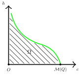
Figure 1: The green curve represents the mapping $c\mapsto m_{c}$ and the shadow region is the intersection of $\Omega$ and $(0,\infty)^{2}$, which corresponds to the set $\mathcal{A}$ due to Lemma 3.8 (ii).

Remark 3.7.

By modifying the arguments in [6, Lem. 5.6] and [38, Lem. 3.3] one is able to show

$$m_{0}=\infty,\quad m_{Q}=0.$$ (3.48)

Nevertheless, the precise values of $m_{0}$ and $m_{Q}$ have no impact on the scattering result; All we need here is the monotonicity and continuity of the curve $c\mapsto m_{c}$. We will therefore postpone the proof to A. ∎

We end this section by establishing some useful properties of the MEI-functional $\mathcal{D}$.

Lemma 3.8.

Suppose that $v\in H^{1}(\mathbb{R}^{2})$ and satisfies $\mathcal{K}(v)\geq 0$. Then

• $\mathcal{D}(v)=0$ if and only if $u=0$.

• $0<\mathcal{D}(v)<\infty$ if and only if $v\in\mathcal{A}$.

• If $u$ is a solution of (1.2) with $u(t_{0})\in\mathcal{A}$, then $\mathcal{D}(u(t))=\mathcal{D}(u(t_{0}))$ for all $t\in I_{\max}$.

• Let $u_{1},u_{2}\in\mathcal{A}$ with $\mathcal{M}(u_{1})\leq\mathcal{M}(u_{2})$ and $\mathcal{H}(u_{1})\leq\mathcal{H}(u_{2})$. Then $\mathcal{D}(u_{1})\leq\mathcal{D}(u_{2})$. If additionally either $\mathcal{M}(u_{1})<\mathcal{M}(u_{2})$ or $\mathcal{H}(u_{1})<\mathcal{H}(u_{2})$, then $\mathcal{D}(u_{1})<\mathcal{D}(u_{2})$.

• Let $\mathcal{D}_{0}\in(0,\infty)$. Then

  $$\|\nabla u\|^{2}_{2} \sim_{\mathcal{D}_{0}}\mathcal{H}(u),$$ (3.49)

  $$\|u\|^{2}_{H^{1}} \sim_{\mathcal{D}_{0}}\mathcal{H}(u)+\mathcal{M}(u)\sim_{\mathcal{D}_{0}}\mathcal{D}(u)$$ (3.50)

  uniformly for all $u\in\mathcal{A}$ with $\mathcal{D}(u)\leq\mathcal{D}_{0}$.

• Let $\mathcal{D}_{0}\in(0,\infty)$. Then

  $$m_{\mathcal{M}(u)}-\mathcal{H}(u)\gtrsim_{\mathcal{D}_{0}}1$$ (3.51)

  uniformly for all $u\in\mathcal{A}$ with $\mathcal{D}(u)\leq\mathcal{D}_{0}$.

Proof.

• It is trivial that $v=0$ implies $\mathcal{D}(v)=0$. Suppose now $\mathcal{D}(v)=0$. Since $\mathcal{K}(v)\geq 0$, we infer from Lemma 3.2 that $\mathcal{H}(v)\geq 0$. In this case, $\mathcal{D}(v)=0$ can only happen when $v=0$.

• It is trivial that $v\in\mathcal{A}$ implies $\mathcal{D}(v)<\infty$. By Lemma 3.2 we also know that $\mathcal{H}(v)>0$ for $v\in\mathcal{A}$, which implies $\mathcal{D}(v)>0$ by the definition of $\mathcal{D}$. Now let $0<\mathcal{D}(v)<\infty$. Then $\mathcal{M}(v)\in(0,{\mathcal{M}(Q)})$. By definition of $\mathcal{D}$ we also know that $\mathcal{H}(v)<m_{\mathcal{M}(v)}$. Using the definition of $m_{\mathcal{M}(v)}$ we conclude that $\mathcal{K}(v)>0$ (under the precondition $\mathcal{K}(v)\geq 0$) and therefore $v\in\mathcal{A}$.

• This follows immediately from the conservation of mass and energy of the NLS flow, the definition of $\mathcal{D}$ and Lemma 3.5.

• This follows from the fact that $c\mapsto m_{c}$ is monotone decreasing on $(0,{\mathcal{M}(Q)})$ and the definition of $\mathcal{D}$.

• Since $u\in\mathcal{A}$, we know that $\mathcal{M}(u)\in(0,\mathcal{M}(Q))$ and using Lemma 3.2 also $\mathcal{H}(u)\in(0,m_{\mathcal{M}(u)})$. Thus

  $$\,\mathrm{dist}\Big{(}(\mathcal{M}(u),\mathcal{H}(u)),\Omega^{c}\Big{)}$$

  $$\leq \,\mathrm{dist}\Big{(}(\mathcal{M}(u),\mathcal{H}(u)),(\mathcal{M}(Q),\mathcal{H}(u))\Big{)}=\mathcal{M}(Q)-\mathcal{M}(u).$$ (3.52)

  Since $\mathcal{H}(u)\geq 0$, we have

  $$\mathcal{D}(u)\geq\frac{\mathcal{M}(u)}{\mathcal{M}(Q)-\mathcal{M}(u)},$$ (3.53)

  which implies

  $$\frac{1}{\mathcal{D}(u)+1}\leq\frac{\mathcal{M}(Q)-\mathcal{M}(u)}{\mathcal{M}(Q)}=1-\frac{\mathcal{M}(u)}{\mathcal{M}(Q)}.$$ (3.54)

  Since $\mathcal{K}(u)>0$, we have

  $$\mathcal{D}(u)\geq \,\mathcal{H}(u)>\mathcal{H}(u)-\frac{1}{4}\mathcal{K}(u)$$

  $$= \,\frac{1}{8}(2\|\nabla u\|_{2}^{2}-\|u\|_{4}^{4})$$

  $$\geq \,\frac{1}{4}\Big{(}1-\frac{\mathcal{M}(u)}{{\mathcal{M}(Q)}}\Big{)}\|\nabla u\|_{2}^{2}$$

  $$\geq \,\frac{\|\nabla u\|_{2}^{2}}{4(\mathcal{D}(u)+1)},$$ (3.55)

  therefore $\|\nabla u\|_{2}^{2}\lesssim_{\mathcal{D}_{0}}\mathcal{H}(u)$. Combining with (3.9) and (iii) we have

  $$\|\nabla u\|_{2}^{2} \sim_{\mathcal{D}_{0}}\mathcal{H}(u),$$ (3.56)

  $$\|u\|_{H^{1}}^{2} \sim_{\mathcal{D}_{0}}\mathcal{H}(u)+\mathcal{M}(u).$$ (3.57)

  It remains to show $\mathcal{H}(u)+\mathcal{M}(u)\sim_{\mathcal{D}_{0}}\mathcal{D}(u)$. Using (3.53) and ((v)) we infer that

  $$\mathcal{H}(u)+\mathcal{M}(u)\sim_{\mathcal{D}_{0}}\|u\|^{2}_{H^{1}}\lesssim_{\mathcal{D}_{0}}\mathcal{D}(u).$$ (3.58)

  To show $\mathcal{D}(u)\lesssim_{\mathcal{D}_{0}}\mathcal{H}(u)+\mathcal{M}(u)$ we discuss the following different cases: If $\mathcal{M}(u)\geq\frac{1}{2}\mathcal{M}(Q)$, then using the fact that $\mathcal{H}(u)\geq 0$ we have

  $$\mathrm{dist}\Big{(}(\mathcal{M}(u),\mathcal{H}(u)),\Omega^{c}\Big{)}\geq\frac{\mathcal{M}(u)}{\mathcal{D}_{0}}\geq\frac{\mathcal{M}(Q)}{2\mathcal{D}_{0}},$$ (3.59)

  which implies

  $$\mathcal{D}(u)\leq\frac{2\mathcal{D}_{0}}{\mathcal{M}(Q)}\Big{(}\mathcal{M}(u)+\mathcal{H}(u)\Big{)}+\mathcal{H}(u).$$ (3.60)

  If $\mathcal{M}(u)\leq\frac{1}{2}\mathcal{M}(Q)$ and $\mathcal{H}(u)\geq\frac{1}{2}m_{\frac{1}{2}\mathcal{M}(Q)}$, then analogously we obtain

  $$\mathcal{D}(u)\leq\frac{2\mathcal{D}_{0}}{m_{\frac{1}{2}\mathcal{M}(Q)}}\Big{(}\mathcal{M}(u)+\mathcal{H}(u)\Big{)}+\mathcal{H}(u).$$ (3.61)

  If $\mathcal{M}(u)\leq\frac{1}{2}\mathcal{M}(Q)$ and $\mathcal{H}(u)\leq\frac{1}{2}m_{\frac{1}{2}\mathcal{M}(Q)}$, then using the monotonicity of $c\mapsto m_{c}$ we have

  $$\mathrm{dist}\Big{(}(\mathcal{M}(u),\mathcal{H}(u)),\Omega^{c}\Big{)}\geq\mathrm{dist}\Big{(}\Big{(}\frac{1}{2}\mathcal{M}(Q),\frac{1}{2}m_{\frac{1}{2}\mathcal{M}(Q)}\Big{)},\Omega^{c}\Big{)}=:\alpha_{0}>0.$$ (3.62)

  Therefore

  $$\mathcal{D}(u)\leq\frac{1}{\alpha_{0}}\Big{(}\mathcal{M}(u)+\mathcal{H}(u)\Big{)}+\mathcal{H}(u),$$ (3.63)

  which completes the proof of (v).

• If this were not the case, then we could find a sequence $(u_{n})_{n}\subset\mathcal{A}$ such that

  $$m_{\mathcal{M}(u_{n})}-\mathcal{H}(u_{n})=o_{n}(1),$$ (3.64)

  which implies

  $$\mathrm{dist}\Big{(}\Big{(}\mathcal{M}(u_{n}),\mathcal{H}(u_{n})\Big{)},\Omega^{c}\Big{)}\leq \,\mathrm{dist}\Big{(}\Big{(}\mathcal{M}(u_{n}),\mathcal{H}(u_{n})\Big{)},\Big{(}\mathcal{M}(u_{n}),m_{\mathcal{M}(u_{n})}\Big{)}\Big{)}$$

  $$= \,m_{\mathcal{M}(u_{n})}-\mathcal{H}(u_{n})=o_{n}(1).$$ (3.65)

  If $\mathcal{M}(u_{n})\gtrsim 1$, then

  $$\mathcal{D}(u_{n})\gtrsim\frac{1}{o_{n}(1)},$$ (3.66)

  contradicting $\mathcal{D}(u_{n})\leq\mathcal{D}_{0}$. If $\mathcal{M}(u_{n})=o_{n}(1)$, then by the monotonicity of $c\mapsto m_{c}$ and (3.64) we know that $\mathcal{H}(u_{n})\gtrsim 1$ and similarly we may again derive the contradiction (3.66).

∎

4 Existence of the minimal blow-up solution

We define

$$\tau(\mathcal{D}_{0}):=\sup\Big{\{} \|\langle\nabla\rangle^{\frac{1}{2}}\psi\|_{{L_{t,x}^{4}}(I_{\max})}:$$

$$\quad\quad\quad\quad\text{$\psi$ is solution of \eqref{NLS}, }\psi(0)\in{\mathcal{A}},\mathcal{D}(\psi(0))\leq\mathcal{D}_{0}\Big{\}}$$ (4.1)

and

$$\mathcal{D}^{*} :=\sup\{\mathcal{D}_{0}>0:\tau(\mathcal{D}_{0})<\infty\}.$$ (4.2)

By Lemma 2.1, Remark 2.2 and Lemma 3.8 (v) we know that $\tau(\mathcal{D}_{0})<\infty$ for sufficiently small $\mathcal{D}_{0}$. We therefore assume that $\mathcal{D}^{*}<\infty$ and aim to derive a contradiction, which will imply $\mathcal{D}^{*}=\infty$ and the desired proof is complete in view of Lemma 3.8 (ii). By the inductive hypothesis we may find a sequence $(\psi_{n})_{n}$ with $(\psi_{n}(0))_{n}\subset{\mathcal{A}}$ which are solutions of (1.2) with maximal lifespan $(I_{n})_{n}$ such that

$$\lim_{n\to\infty}\|\langle\nabla\rangle^{\frac{1}{2}}\psi_{n}\|_{{L_{t,x}^{4}}(I_{n})}=\infty,$$ (4.3)

$$\lim_{n\to\infty}\mathcal{D}(\psi_{n}(0))=\mathcal{D}^{*}.$$ (4.4)

Up to a subsequence we may also assume that

$$(\mathcal{M}(\psi_{n}(0)),\mathcal{H}(\psi_{n}(0)))\to(\mathcal{M}_{0},\mathcal{H}_{0})\quad\text{as $n\to\infty$}.$$ (4.5)

By continuity of $\mathcal{D}$ and finiteness of $\mathcal{D}^{*}$ we know that

$$\mathcal{D}^{*} =\mathcal{D}(\mathcal{M}_{0},\mathcal{H}_{0}),$$ (4.6)

$$\mathcal{M}_{0} \in(0,\mathcal{M}(Q)),$$ (4.7)

$$\mathcal{H}_{0} \in[0,m_{\mathcal{M}_{0}}).$$ (4.8)

By Lemma 3.8 (v) we deduce that $(\psi_{n}(0))_{n}$ is a bounded sequence in $H^{1}(\mathbb{R}^{2})$. Using Lemma 2.4 applied to $(\psi_{n}(0))_{n}$ we infer that there exist some number $K^{*}\in\mathbb{N}\cup\{\infty\}$, a sequence of nonzero linear profiles $(\phi^{j})_{1\leq j\leq K^{*}}\subset L^{2}(\mathbb{R}^{2})$, a sequence of symmetry parameters $(\lambda_{n}^{j},t_{n}^{j},x_{n}^{j},\xi_{n}^{j})_{n\in\mathbb{N},1\leq j\leq K^{*}}\subset(0,\infty)\times\mathbb{R}\times\mathbb{R}^{2}\times\mathbb{R}^{2}$ with $\sup_{n\in\mathbb{N}}|\xi_{n}^{j}|\lesssim_{j}1$ and a sequence of remainders $(w_{n}^{k})_{n\in\mathbb{N},1\leq k\leq K^{*}}\subset H^{1}(\mathbb{R}^{2})$ such that

• The parameters $(\lambda_{n}^{j},t_{n}^{j},x_{n}^{j},\xi_{n}^{j})_{n,j}$ satisfy

  $$\lim_{n\to\infty} \Big{\{}\Big{|}\log\frac{\lambda_{n}^{j}}{\lambda_{n}^{l}}\Big{|}+\frac{|t_{n}^{j}-t_{n}^{l}|}{(\lambda_{n}^{j})^{2}}$$

  $$\quad\quad\quad+\lambda_{n}^{j}|\xi_{n}^{j}-\xi_{n}^{l}|+\frac{|x_{n}^{j}-x_{n}^{l}+2t_{n}^{j}(\xi_{n}^{j}-\xi_{n}^{l})|}{\lambda_{n}^{j}}\Big{\}}=\infty$$ (4.9)

  for all finite $1\leq j,l\leq K^{*}$ with $j\neq l$. Moreover,

  $$\lim_{n\to\infty}\lambda_{n}^{j} =\lambda^{j}_{\infty}\in\{1,\infty\},$$ (4.10)

  $$\lambda_{n}^{j} \equiv 1\quad\text{if $\lambda_{\infty}^{j}=1$}.$$ (4.11)

• There exists some $\theta\in(0,1)$ such that for any finite $1\leq k\leq K^{*}$ we have the decomposition

  $$\psi_{n}(0)=\sum_{j=1}^{k}T_{n}^{j}P_{n}^{j}\phi^{j}+w_{n}^{k},$$ (4.12)

  where

  $$T_{n}^{j}u(x):=e^{ix\cdot\xi_{n}^{j}}e^{-t_{n}^{j}\Delta}(\lambda_{n}^{j})^{-1}u\Big{(}(\lambda_{n}^{j})^{-1}(\cdot-x_{n}^{j})\Big{)}(x)$$ (4.13)

  and

  $$P_{n}^{j}\phi^{j}=\left\{\begin{array}[]{ll}\phi^{j},&\text{if $\lambda_{\infty}^{j}=1$},\\ P_{\leq(\lambda_{n}^{j})^{\theta}}\phi^{j},&\text{if $\lambda_{\infty}^{j}=\infty$}.\end{array}\right.$$ (4.14)

  Moreover, if $\lambda^{j}_{\infty}=1$, then $\xi_{n}^{j}\equiv 0$ and $\phi^{j}\in H^{1}(\mathbb{R}^{2})$.

• The remainders $(w_{n}^{k})_{n,k}$ satisfy

  $$\lim_{k\to K^{*}}\lim_{n\to\infty}\|\langle\nabla\rangle^{\frac{1}{2}}e^{it\Delta}w_{n}^{k}\|_{{L_{t,x}^{4}}(\mathbb{R})}=0.$$ (4.15)

• The following orthogonal properties are satisfied: for $s\in\{0,1\}$ and finite $1\leq J\leq K^{*}$ we have

  $$\||\nabla|^{s}\psi_{n}\|_{2}^{2} =\sum_{j=1}^{J}\||\nabla|^{s}T_{n}^{j}P_{n}^{j}\phi^{j}\|_{2}^{2}+\||\nabla|^{s}w_{n}^{J}\|_{2}^{2}+o_{n}(1),$$ (4.16)

  $$\mathcal{H}(\psi_{n}) =\sum_{j=1}^{J}\mathcal{H}(T_{n}^{j}P_{n}^{j}\phi^{j})+\mathcal{H}(w_{n}^{J})+o_{n}(1),$$ (4.17)

  $$\mathcal{I}(\psi_{n}) =\sum_{j=1}^{J}\mathcal{I}(T_{n}^{j}P_{n}^{j}\phi^{j})+\mathcal{I}(w_{n}^{J})+o_{n}(1),$$ (4.18)

  $$\mathcal{K}(\psi_{n}) =\sum_{j=1}^{J}\mathcal{K}(T_{n}^{j}P_{n}^{j}\phi^{j})+\mathcal{K}(w_{n}^{J})+o_{n}(1).$$ (4.19)

Lemma 4.1.

There exists a global solution $u_{c}$ of (1.2) such that

$$(\mathcal{D}(u_{c}),\mathcal{M}(u_{c}),\mathcal{H}(u_{c}))=(\mathcal{D}^{*},\mathcal{M}_{0},\mathcal{H}_{0})$$ (4.20)

and

$$\|\langle\nabla\rangle^{\frac{1}{2}}u_{c}\|_{{L_{t,x}^{4}}(\mathbb{R})}=\infty.$$ (4.21)

Proof.

We first show that for a given nonzero linear profile $\phi^{j}$ we have

$$\mathcal{H}(T_{n}^{j}P_{n}^{j}\phi^{j}) >0,$$ (4.22)

$$\mathcal{K}(T_{n}^{j}P_{n}^{j}\phi^{j}) >0$$ (4.23)

for all sufficiently large $n=n(j)\in\mathbb{N}$. Since $\phi^{j}\neq 0$ we know that $T_{n}^{j}P_{n}^{j}\phi^{j}\neq 0$ for sufficiently large $n$. Suppose now that (4.23) does not hold. Up to a subsequence we may assume that $\mathcal{K}(T_{n}^{j}P_{n}^{j}\phi^{j})\leq 0$ for all sufficiently large $n$. By the non-negativity of $\mathcal{I}$, (4.18) and (3.51) we know that there exists some sufficiently small $\delta>0$ depending on $\mathcal{D}^{*}$ and some sufficiently large $N_{1}$ such that for all $n>N_{1}$ we have

$${\tilde{m}}_{\mathcal{M}(T_{n}^{j}P_{n}^{j}\phi^{j})} \leq\mathcal{I}(T_{n}^{j}P_{n}^{j}\phi^{j})\leq\mathcal{I}(\psi_{n}(0))+\delta$$

$$\leq\mathcal{H}(\psi_{n}(0))+\delta\leq m_{\mathcal{M}(\psi_{n}(0))}-2\delta,$$ (4.24)

where ${\tilde{m}}$ is the quantity defined by Lemma 3.6. By continuity of $c\mapsto m_{c}$ we also know that for sufficiently large $n$ we have

$$m_{\mathcal{M}(\psi_{n}(0))}-2\delta\leq m_{\mathcal{M}_{0}}-\delta.$$ (4.25)

Using (4.16) we deduce that for any $\varepsilon>0$ there exists some large $N_{2}$ such that for all $n>N_{2}$ we have

$$\mathcal{M}(T_{n}^{j}P_{n}^{j}\phi^{j})\leq\mathcal{M}_{0}+\varepsilon.$$ (4.26)

From the continuity and monotonicity of $c\mapsto m_{c}$ and Lemma 3.6, we may choose some sufficiently small $\varepsilon$ to see that

$${\tilde{m}}_{\mathcal{M}(T_{n}^{j}P_{n}^{j}\phi^{j})}=m_{\mathcal{M}(T_{n}^{j}P_{n}^{j}\phi^{j})}\geq m_{\mathcal{M}_{0}+\varepsilon}\geq m_{\mathcal{M}_{0}}-\frac{\delta}{2}.$$ (4.27)

Now (4), (4.25) and (4.27) yield a contradiction. Thus (4.23) holds, which combining with Lemma 3.2 also yields (4.22). Similarly, for each $j\in\mathbb{N}$ we have

$$\mathcal{H}(w_{n}^{j}) \geq 0,$$ (4.28)

$$\mathcal{K}(w_{n}^{j}) \geq 0$$ (4.29)

for sufficiently large $n$. Now using (4.5) we have for any $k\in\mathbb{N}$

$$\mathcal{M}_{0} =\sum_{j=1}^{k}\mathcal{M}(T_{n}^{j}P_{n}^{j}\phi^{j})+\mathcal{M}(w_{n}^{k})+o_{n}(1),$$ (4.30)

$$\mathcal{H}_{0} =\sum_{j=1}^{k}\mathcal{H}(T_{n}^{j}P_{n}^{j}\phi^{j})+\mathcal{H}(w_{n}^{k})+o_{n}(1).$$ (4.31)

From (4.30) and (4.31) we infer that two different scenarios will potentially take place: either

$$\sup_{j\in\mathbb{N}}\lim_{n\to\infty}\mathcal{M}(T_{n}^{j}P_{n}^{j}\phi^{j}) =\mathcal{M}_{0}\text{ and}$$

$$\sup_{j\in\mathbb{N}}\lim_{n\to\infty}\mathcal{H}(T_{n}^{j}P_{n}^{j}\phi^{j}) =\mathcal{H}_{0},$$ (4.32)

or there exists some $\delta>0$ such that

$$\sup_{j\in\mathbb{N}}\lim_{n\to\infty}\mathcal{M}(T_{n}^{j}P_{n}^{j}\phi^{j}) \leq\mathcal{M}_{0}-\delta\text{ or}$$

$$\sup_{j\in\mathbb{N}}\lim_{n\to\infty}\mathcal{H}(T_{n}^{j}P_{n}^{j}\phi^{j}) \leq\mathcal{H}_{0}-\delta.$$ (4.33)

We show that starting from (4.32) one is able to derive a minimal blow-up solution $u_{c}$ which satisfies (4.20) and (4.21), while from (4.33) we get a contradiction. We begin firstly with (4.32). In this case, since the summands in (4.30) and (4.31) are non-negative for fixed $j$ and sufficiently large $n$, it is necessary that there exists exactly one non-trivial linear profile $\phi^{j}=\phi^{1}$ and

$$\psi_{n}(0)=T_{n}^{1}P_{n}^{1}\phi^{1}+w_{n}^{1}.$$ (4.34)

Particularly, from (4.30) and (4.31) it follows

$$\lim_{n\to\infty}\mathcal{M}(T_{n}^{1}P_{n}^{1}\phi^{1}) =\mathcal{M}_{0},$$ (4.35)

$$\lim_{n\to\infty}\mathcal{H}(T_{n}^{1}P_{n}^{1}\phi^{1}) =\mathcal{H}_{0},$$ (4.36)

$$\lim_{n\to\infty}\|w_{n}^{1}\|_{2} =0,$$ (4.37)

$$\lim_{n\to\infty}\mathcal{H}(w_{n}^{1}) =0.$$ (4.38)

Combining with Lemma 3.8 (v), (4.38) also implies

$$\lim_{n\to\infty}\|\nabla w_{n}^{1}\|_{2}=0,$$ (4.39)

thus together with (4.37) we deduce that

$$\lim_{n\to\infty}\|w_{n}^{1}\|_{H^{1}}=0.$$ (4.40)

Using (4.16) we see that

$$\limsup_{n\to\infty}\|T_{n}^{1}P_{n}^{1}\phi^{1}\|_{H^{1}}<\infty.$$ (4.41)

From (4.40) we infer that

$$\limsup_{n\to\infty}\|\langle\nabla\rangle^{\frac{1}{2}}(\psi_{n}(0)-T_{n}^{1}P_{n}^{1}\phi^{1})\|_{2}\lesssim\lim_{n\to\infty}\|w_{n}^{1}\|_{H^{1}}=0.$$ (4.42)

Since $\mathcal{M}_{0}<\mathcal{M}(Q)$, we obtain from (4.30) that

$$\mathcal{M}(T_{n}^{1}P_{n}^{1}\phi^{1})\leq\frac{\mathcal{M}_{0}+\mathcal{M}(Q)}{2}<\mathcal{M}(Q)$$ (4.43)

for sufficiently large $n$, hence Lemma 2.5 is applicable. If $\lambda^{1}_{\infty}=\infty$, then using Lemma 2.5 we know that for sufficiently large $n$, there exists a global and scattering solution $v_{n}$ of (1.2) with

$$v_{n}(0)=T_{n}^{1}P_{n}^{1}\phi^{1}.$$ (4.44)

Finally, using Strichartz and (4.40) we see that

$$\lim_{n\to\infty}\|\langle\nabla\rangle^{\frac{1}{2}}e^{it\Delta}(\psi_{n}(0)-T_{n}^{1}P_{n}^{1}\phi^{1})\|_{L_{t,x}^{4}(\mathbb{R})}\lesssim\lim_{n\to\infty}\|w_{n}^{1}\|_{H^{1}}=0.$$ (4.45)

Therefore, the conditions (2.8) to (2.11) of Lemma 2.3 are satisfied and by setting the error term $e=0$ we infer that

$$\limsup_{n\to\infty}\|\langle\nabla\rangle^{\frac{1}{2}}\psi_{n}\|_{{L_{t,x}^{4}}(\mathbb{R})}<\infty,$$ (4.46)

which contradicts (4.3). Hence $\lambda^{1}_{\infty}=1$ and $T_{n}^{1}P_{n}^{1}\phi^{1}=T_{n}^{1}\phi^{1}$. Suppose that $\lim_{n\to\infty}t_{n}^{1}=t_{\infty}^{1}$. We then define $u_{c}$ as the solution of the integral equation

$$u_{c}(t)=e^{it\Delta}\phi^{1}+i\int_{-t_{\infty}^{1}}^{t}(|u_{c}|^{2}u_{c}+|u_{c}|^{4}u_{c})(s)\,ds,$$ (4.47)

whose local existence near $-t_{\infty}^{1}$ is guaranteed by Lemma 2.1. (4.20) follows already from (4.30), (4.31) and the continuity of $\mathcal{D}$. If (4.21) does not hold, then by Lemma 2.1 we know that $u_{c}$ must be a global solution. We can therefore define

$$\tilde{v}_{n}:=u_{c}(t-t_{n}^{1},x-x_{n}^{1}).$$ (4.48)

By time and space translation invariance we infer that $\tilde{v}_{n}$ is a solution of (1.2) and

$$\|\langle\nabla\rangle^{\frac{1}{2}}\tilde{v}_{n}\|_{{L_{t,x}^{4}}(\mathbb{R})}=\|\langle\nabla\rangle^{\frac{1}{2}}u_{c}\|_{{L_{t,x}^{4}}(\mathbb{R})}.$$ (4.49)

By the construction of $u_{c}$ we also know that

$$\lim_{n\to\infty}\|\hat{v}_{n}(0)-T_{n}^{1}\phi^{1}\|_{H^{1}}=0.$$ (4.50)

Now as argued previously, we arrive at the contradiction (4.46) again. Finally, we can mimic the proof of [2, Prop. 6.11], words by words, to show that $u_{c}$ is global. We omit the details here. The proof for the first scenario is done.

We now consider the second scenario (4.33). In this case, for each $j\in\mathbb{N}$ we must have

$$\mathcal{M}(T_{n}^{j}P_{n}^{j}\phi^{j}) \leq\mathcal{M}_{0}-\frac{\delta}{2}\text{ or }$$

$$\mathcal{H}(T_{n}^{j}P_{n}^{j}\phi^{j}) \leq\mathcal{H}_{0}-\frac{\delta}{2}$$ (4.51)

for sufficiently large $n$. Define

$$\mathcal{D}_{1} :=\mathcal{D}(\mathcal{M}_{0}-\frac{\delta}{2},\mathcal{H}_{0}+\varepsilon_{1}(\delta)),$$

$$\mathcal{D}_{2} :=\mathcal{D}(\mathcal{M}_{0}+\varepsilon_{2}(\delta),\mathcal{H}_{0}-\frac{\delta}{2})$$

for some $\varepsilon_{1}(\delta),\varepsilon_{2}(\delta)>0$ such that $\mathcal{D}_{1},\mathcal{D}_{2}<\mathcal{D}^{*}$. This is possible due to Lemma 3.8 (iv) and the continuity of $\mathcal{D}$. Thus by the inductive hypothesis (4.2) we infer that there exist nonlinear profiles $v_{n}^{j}$ which are global solutions of (1.2) with $v_{n}^{j}(0)=T_{n}^{j}P_{n}^{j}\phi^{j}$ and

$$\|\langle\nabla\rangle^{\frac{1}{2}}v_{n}^{j}\|_{L_{t,x}^{4}(\mathbb{R})}\leq\max\{\tau(\mathcal{D}_{1}),\tau(\mathcal{D}_{2})\}$$ (4.53)

for each $j\in\mathbb{N}$ and all sufficiently $n$, where $\tau$ is the quantity defined by (4). Having defined the nonlinear profiles $v_{n}^{j}$, we now define the proxy $\Psi_{n}^{K}$ by

$$\Psi_{n}^{K}:=\sum_{j=1}^{K}v_{n}^{j}+e^{it\Delta}w_{n}^{K},$$ (4.54)

with some sufficiently large $K$ and $n=n(K)$ to be chosen later. Since the error analysis is available for all models regardless of the signs of the nonlinearities, we are able to invoke the error analysis given in the proof of [15, Prop. 5.2] to see that (2.8) to (2.12) are satisfied for some sufficiently large $K$ and $n=n(K)$, where we also replace [15, Lem. 2.3] by Lemma 3.8 (v). Using Lemma 2.3 we conclude the contradiction (4.46) again. This completes the desired proof. ∎

5 Extinction of the minimal blow-up solution

We close in this section the proof of Theorem 1.2 by showing the contradiction that the minimal blow-up solution $u_{c}$ given by Lemma 4.1 must be zero. To proceed, we still need the following lemma which can be proved as in [20, 27] verbatim, so we omit the details of the proof here.

Lemma 5.1 ([20, 27]).

Let $u_{c}$ be the minimal blow-up solution given by Lemma 4.1. Then

• For each $\varepsilon>0$, there exists $R=R(\varepsilon)>0$ so that

  $$\int_{|x+x(t)|\geq R}|\nabla u_{c}(t)|^{2}+|u_{c}(t)|^{2}+|u_{c}|^{4}+|u_{c}|^{6}\,dx\leq\varepsilon\quad\forall\,t\in[0,\infty).$$ (5.1)

• The center function $x(t)$ obeys the decay condition $x(t)=o(t)$ as $t\to\infty$.

Proof of Theorem 1.2

We will show the contradiction that the minimal blow-up solution $u_{c}$ given by Lemma 4.1 is equal to zero, which will finally imply Theorem 1.2. Let $\chi$ be a smooth radial cut-off function satisfying

$$\chi(x)=\left\{\begin{array}[]{ll}|x|^{2},&\text{if $|x|\leq 1$},\\ 0,&\text{if $|x|\geq 2$}.\end{array}\right.$$ (5.4)

Define also the local virial action

$$z_{R}(t):=\int R^{2}\chi\Big{(}\frac{x}{R}\Big{)}|u_{c}(t,x)|^{2}\,dx.$$ (5.5)

Direct calculation yields

$$\partial_{t}z_{R}(t)= \,2\,\mathrm{Im}\int R\nabla\chi\Big{(}\frac{x}{R}\Big{)}\cdot\nabla u_{c}(t)\bar{u}_{c}(t)\,dx,$$ (5.6)

$$\partial_{tt}z_{R}(t)= \,4\int\partial^{2}_{jk}\chi\Big{(}\frac{x}{R}\Big{)}\partial_{j}u_{c}\partial_{k}\bar{u}_{c}-\frac{1}{R^{2}}\int\Delta^{2}\chi\Big{(}\frac{x}{R}\Big{)}|u_{c}|^{2}$$

$$\,-\int\Delta\chi\Big{(}\frac{x}{R}\Big{)}|u_{c}|^{4}\,dx-\frac{4}{3}\int\Delta\chi\Big{(}\frac{x}{R}\Big{)}|u_{c}|^{6}\,dx.$$ (5.7)

Here we used the Einstein summation for the repeated indices. We then obtain that

$$\partial_{tt}z_{R}(t)=8\mathcal{K}(u_{c})+A_{R}(u_{c}(t)),$$ (5.8)

where

$$A_{R}(u_{c}(t))= \,4\int\Big{(}\partial^{2}_{j}\chi\Big{(}\frac{x}{R}\Big{)}-2\Big{)}|\partial_{j}u_{c}|^{2}+4\sum_{j\neq k}\int_{R\leq|x|\leq 2R}\partial^{2}_{jk}\chi\Big{(}\frac{x}{R}\Big{)}\partial_{j}u_{c}\partial_{k}\bar{u}_{c}$$

$$\,-\frac{1}{R^{2}}\int\Delta^{2}\chi\Big{(}\frac{x}{R}\Big{)}|u_{c}|^{2}-\int\Big{(}\Delta\chi\Big{(}\frac{x}{R}\Big{)}-4\Big{)}|u_{c}|^{4}\,dx$$

$$\,-\frac{4}{3}\int\Big{(}\Delta\chi\Big{(}\frac{x}{R}\Big{)}-4\Big{)}|u_{c}|^{6}\,dx.$$ (5.9)

We can roughly estimate $A_{R}(u_{c}(t))$ by

$$|A_{R}(u_{c}(t))|\leq C_{1}\int_{|x|\geq R}|\nabla u_{c}(t)|^{2}+\frac{1}{R^{2}}|u_{c}(t)|^{2}+|u_{c}|^{4}+|u_{c}|^{6}$$ (5.10)

for some $C_{1}>0$. Since $\mathcal{M}(u_{c})=\mathcal{M}_{0}<\mathcal{M}(Q)$, we may assume that $\mathcal{M}(u_{c})=(1-\delta)\mathcal{M}(Q)$ for some $\delta\in(0,1)$. Using (3.26) we obtain that

$$\mathcal{K}(u_{c}(t)) \geq\min\Big{\{}\delta\mathcal{H}(u_{c}(0)),\,\Big{(}\Big{(}\frac{2}{\delta}\Big{)}^{{\frac{1}{2}}}-1\Big{)}^{-1}\Big{(}m_{\mathcal{M}(u_{c}(0))}-\mathcal{H}(u_{c}(0))\Big{)}\Big{\}}$$

$$=:4^{-1}\eta_{1}$$ (5.11)

for all $t\in\mathbb{R}$. Using Lemma 5.1 (i) we know that there exists some $R_{0}\geq 1$ such that

$$\int_{|x+x(t)|\geq R_{0}}|\nabla u_{c}|^{2}+|u_{c}|^{2}+|u_{c}|^{4}+|u_{c}|^{6}\,dx\leq\frac{\eta}{C_{1}}.$$ (5.12)

Thus for any $R\geq R_{0}+\sup_{t\in[t_{0},t_{1}]}|x(t)|$ with some to be determined $t_{0},t_{1}\in[0,\infty)$, we obtain that

$$\partial_{tt}z_{R}(t)\geq\eta_{1}$$ (5.13)

for all $t\in[t_{0},t_{1}]$. By Lemma 5.1 (ii), for some to be determined small $\eta_{2}$ we can choose sufficiently large $t_{0}$ such that $|x(t)|\leq\eta_{2}t$ for all $t\geq t_{0}$. Now set $R=R_{0}+\eta_{2}t_{1}$. Integrating (5.13) over $[t_{0},t_{1}]$ yields

$$\partial_{t}z_{R}(t_{1})-\partial_{t}z_{R}(t_{0})\geq\eta_{1}(t_{1}-t_{0}).$$ (5.14)

Using (5.6), Cauchy-Schwarz and Lemma 3.8 (v) we have

$$|\partial_{t}z_{R}(t)|\leq C_{2}\mathcal{D}^{*}R=C_{2}\mathcal{D}^{*}(R_{0}+\eta_{2}t_{1})$$ (5.15)

for some $C_{2}=C_{2}(\mathcal{D}^{*})>0$. (5.14) and (5.15) give us

$$2C_{2}\mathcal{D}^{*}(R_{0}+\eta_{2}t_{1})\geq\eta_{1}(t_{1}-t_{0}).$$ (5.16)

Setting $\eta_{2}=(4C_{2}\mathcal{D}^{*})^{-1}$ and then sending $t_{1}$ to infinity we obtain a contradiction unless $\eta_{1}=0$, which implies $\mathcal{H}_{0}=\mathcal{H}(u_{c})=0$. From Lemma 3.8 (v) we conclude that $\nabla u_{c}=0$, which implies $u_{c}=0$. This completes the proof. $\square$

6 A solely mass-determining scattering threshold for the problem (1.7)

In this section we continue our discussion on the NLS (1.7). Our aim is to impose a solely mass-determining scattering threshold for (1.7) which is similar to the one given in Theorem 1.2. Our starting point is the following result given in [35, 38]:

Theorem 6.1 ([35, 38]).

Let $d\geq 3$. Then

• Existence of ground state: For any $c\in(0,\infty)$ the variational problem (1.5) corresponding to (1.7) has a minimizer $S_{c}$ with $\mathcal{H}(S_{c})=m_{c}\in(0,d^{-1}\mathcal{S}^{\frac{d}{2}})$. Moreover, $S_{c}$ is a solution of (1.4) with some $\omega>0$. In addition, $S_{c}$ can be chosen to be positive and radially symmetric.

• Blow-up criterion: Assume that $u_{0}\in H^{1}(\mathbb{R}^{d})$ satisfies the conditions $\mathcal{H}(u_{0})<m_{\mathcal{M}(u_{0})}$ and $\mathcal{K}(u_{0})<0$. Assume also that $|x|u_{0}\in L^{2}(\mathbb{R}^{d})$. Then the solution $u$ of (1.7) with $u(0)=u_{0}$ blows-up in finite time.

The scattering result can now be formulated as follows:

Theorem 6.2.

Define the set

$$\mathcal{B} :=\{u\in H^{1}(\mathbb{R}^{d}):\mathcal{H}(u)<m_{\mathcal{M}(u)},\mathcal{K}(u)>0\}$$ (6.1)

and assume that $u_{0}\in\mathcal{B}$. Additionally we assume that $u_{0}$ is radially symmetric in the case $d=3$. Then the solution $u$ of (1.7) with $u(0)=u_{0}$ is global and scatters in time.

The proof is a straightforward modification and combination of the variational arguments given in Section 3 and the nonlinear estimates in [2], we therefore omit the details here.

Acknowledgments

The author acknowledges the funding by Deutsche Forschungsgemeinschaft (DFG) through the Priority Programme SPP-1886 (No. NE 21382-1). The author also thanks the anonymous referee sincerely for her/his thorough reading of the manuscript and for many important corrections.

Appendix A Precise values of $m_{0}$ and $m_{Q}$

Proposition A.1.

We have $m_{0}=\infty$ and $m_{Q}=0$.

Proof.

From Theorem 1.1 we know that for any $c\in(0,\mathcal{M}(Q))$, $m_{c}$ has a minimizer $S_{c}$. Therefore

$$\mathcal{H}(S_{c})=m_{c},\quad\mathcal{K}(S_{c})=0,\quad\mathcal{M}(S_{c})=c.$$ (A.1)

Using $\mathcal{K}(S_{c})=0$ and Gagliardo-Nirenberg we infer that

$$\|\nabla S_{c}\|_{2}^{2}=\frac{1}{2}\|S_{c}\|_{4}^{4}+\frac{2}{3}\|S_{c}\|_{6}^{6}\leq c\mathcal{M}(Q)^{-1}\|\nabla S_{c}\|_{2}^{2}+\frac{2c\,{\widehat{\mathrm{C}}_{\mathrm{GN}}}^{-1}}{3}\|\nabla S_{c}\|_{2}^{4},$$ (A.2)

which implies

$$\|\nabla S_{c}\|_{2}^{2}\geq\frac{3{\widehat{\mathrm{C}}_{\mathrm{GN}}}}{2}\Big{(}\frac{1}{c}-\frac{1}{\mathcal{M}(Q)}\Big{)}.$$ (A.3)

Therefore $\|\nabla S_{c}\|_{2}^{2}\to\infty$ as $c\to 0$. Now we obtain

$$\mathcal{H}(S_{c}) =\mathcal{H}(S_{c})-\frac{1}{4}\mathcal{K}(S_{c})$$

$$=\frac{1}{4}(\|\nabla S_{c}\|_{2}^{2}-\frac{1}{2}\|S_{c}\|_{4}^{4})$$

$$\geq\frac{1}{4}(1-c\mathcal{M}(Q)^{-1})\|\nabla S_{c}\|_{2}^{2}\to\infty$$ (A.4)

as $c\to 0$, which implies $m_{0}=\infty$. Next we show $m_{Q}=0$. Let $(u_{n})_{n}$ be a minimizing sequence for (1.12). By rescaling we may assume that $\mathcal{M}(u_{n})=\delta^{2}\mathcal{M}(Q)$ for $\delta\in(1/2,1)$ which will be sended to one later, and $\|u_{n}\|_{4}\equiv 1$. Then combining with (1.13) we obtain that $\|\nabla u_{n}\|_{2}^{2}=(2\delta^{2})^{-1}+o_{n}(1)$. We then conclude that

$$\mathcal{K}(T_{\lambda}u_{n})=\frac{\lambda^{2}}{2}\Big{(}\frac{1}{\delta^{2}}-1+o_{n}(1)\Big{)}-\frac{2\lambda^{4}}{3}\|u_{n}\|_{6}^{6}.$$ (A.5)

By setting

$$\lambda_{n,\delta}=\Big{(}\frac{3}{4\|u_{n}\|_{6}^{6}}\Big{(}\frac{1}{\delta^{2}}-1+o_{n}(1)\Big{)}\Big{)}^{\frac{1}{2}}$$ (A.6)

we see that $\mathcal{K}(T_{\lambda_{n,\delta}}u_{n})=0$. By Hölder we obtain that

$$\|u_{n}\|_{6}^{6}\geq\mathcal{M}(u_{n})^{-1}\|u_{n}\|_{4}^{8}=\delta^{-2}\mathcal{M}(Q)^{-1}.$$ (A.7)

We now choose $N=N(\delta)\in\mathbb{N}$ such that $|o_{n}(1)|\leq\delta^{-2}-1$ for all $n>N$. Summing up and using the definition of $m_{c}$ we finally conclude that

$$m_{\delta^{2}\mathcal{M}(Q)} \leq\sup_{n>N}\mathcal{H}(T_{\lambda_{n,\delta}}u_{n})=\sup_{n>N}\Big{(}\mathcal{H}(T_{\lambda_{n,\delta}}u_{n})-\frac{1}{2}\mathcal{K}(T_{\lambda_{n,\delta}}u_{n})\Big{)}$$

$$=\sup_{n>N}\frac{1}{6}\|T_{\lambda_{n,\delta}}u_{n}\|_{6}^{6}=\sup_{n>N}\frac{\lambda_{n,\delta}^{4}}{6}\|u_{n}\|_{6}^{6}$$

$$\leq\frac{9}{24}\mathcal{M}(Q)\delta^{-2}(1-\delta^{2})^{2}\to 0$$ (A.8)

as $\delta\to 1$. This proves $m_{Q}=0$. ∎

References

- [1] Akahori, T., Ibrahim, S., Kikuchi, H., and Nawa, H. Existence of a ground state and blow-up problem for a nonlinear Schrödinger equation with critical growth. Differential Integral Equations 25, 3-4 (2012), 383–402.
- [2] Akahori, T., Ibrahim, S., Kikuchi, H., and Nawa, H. Existence of a ground state and scattering for a nonlinear Schrödinger equation with critical growth. Selecta Math. (N.S.) 19, 2 (2013), 545–609.
- [3] Akahori, T., Ibrahim, S., Kikuchi, H., and Nawa, H. Global dynamics above the ground state energy for the combined power type nonlinear Schrödinger equations with energy critical growth at low frequencies, 2019.
- [4] Bégout, P., and Vargas, A. Mass concentration phenomena for the -critical nonlinear Schrödinger equation. Trans. Amer. Math. Soc. 359, 11 (2007), 5257–5282.
- [5] Bellazzini, J., and Jeanjean, L. On dipolar quantum gases in the unstable regime. SIAM J. Math. Anal. 48, 3 (2016), 2028–2058.
- [6] Bellazzini, J., Jeanjean, L., and Luo, T. Existence and instability of standing waves with prescribed norm for a class of Schrödinger-Poisson equations. Proc. Lond. Math. Soc. (3) 107, 2 (2013), 303–339.
- [7] Berestycki, H., and Lions, P.-L. Nonlinear scalar field equations. I. Existence of a ground state. Arch. Rational Mech. Anal. 82, 4 (1983), 313–345.
- [8] Berestycki, H., and Lions, P.-L. Nonlinear scalar field equations. II. Existence of infinitely many solutions. Arch. Rational Mech. Anal. 82, 4 (1983), 347–375.
- [9] Brézis, H., and Nirenberg, L. Positive solutions of nonlinear elliptic equations involving critical Sobolev exponents. Comm. Pure Appl. Math. 36, 4 (1983), 437–477.
- [10] Carles, R., and Keraani, S. On the role of quadratic oscillations in nonlinear Schrödinger equations. II. The -critical case. Trans. Amer. Math. Soc. 359, 1 (2007), 33–62.
- [11] Carles, R., Klein, C., and Sparber, C. On soliton (in-)stability in multi-dimensional cubic-quintic nonlinear schrödinger equations, 2020.
- [12] Carles, R., and Sparber, C. Orbital stability vs. scattering in the cubic-quintic Schrödinger equation. Rev. Math. Phys. 33, 3 (2021), 2150004, 27.
- [13] Cazenave, T. Semilinear Schrödinger equations, vol. 10 of Courant Lecture Notes in Mathematics. New York University, Courant Institute of Mathematical Sciences, New York; American Mathematical Society, Providence, RI, 2003.
- [14] Cazenave, T., and Lions, P.-L. Orbital stability of standing waves for some nonlinear Schrödinger equations. Comm. Math. Phys. 85, 4 (1982), 549–561.
- [15] Cheng, X. Scattering for the mass super-critical perturbations of the mass critical nonlinear Schrödinger equations. Illinois J. Math. 64, 1 (2020), 21–48.
- [16] Cheng, X., Miao, C., and Zhao, L. Global well-posedness and scattering for nonlinear Schrödinger equations with combined nonlinearities in the radial case. J. Differential Equations 261, 6 (2016), 2881–2934.
- [17] Cowan, S., Enns, R. H., Rangnekar, S. S., and Sanghera, S. S. Quasi-soliton and other behaviour of the nonlinear cubic-quintic schrödinger equation. Canadian Journal of Physics 64, 3 (Mar. 1986), 311–315.
- [18] Dodson, B. Global well-posedness and scattering for the mass critical nonlinear Schrödinger equation with mass below the mass of the ground state. Adv. Math. 285 (2015), 1589–1618.
- [19] Dodson, B. Global well-posedness and scattering for the focusing, cubic Schrödinger equation in dimension . Ann. Sci. Éc. Norm. Supér. (4) 52, 1 (2019), 139–180.
- [20] Duyckaerts, T., Holmer, J., and Roudenko, S. Scattering for the non-radial 3D cubic nonlinear Schrödinger equation. Math. Res. Lett. 15, 6 (2008), 1233–1250.
- [21] Gagnon, L. Exact traveling-wave solutions for optical models based on the nonlinear cubic-quintic schrödinger equation. Journal of the Optical Society of America A 6, 9 (Sept. 1989), 1477.
- [22] Jeanjean, L. On the existence of bounded Palais-Smale sequences and application to a Landesman-Lazer-type problem set on . Proc. Roy. Soc. Edinburgh Sect. A 129, 4 (1999), 787–809.
- [23] Keel, M., and Tao, T. Endpoint Strichartz estimates. Amer. J. Math. 120, 5 (1998), 955–980.
- [24] Kenig, C. E., and Merle, F. Global well-posedness, scattering and blow-up for the energy-critical, focusing, non-linear Schrödinger equation in the radial case. Invent. Math. 166, 3 (2006), 645–675.
- [25] Keraani, S. On the defect of compactness for the Strichartz estimates of the Schrödinger equations. J. Differential Equations 175, 2 (2001), 353–392.
- [26] Killip, R., Murphy, J., and Visan, M. Scattering for the cubic-quintic NLS: crossing the virial threshold. SIAM J. Math. Anal. 53, 5 (2021), 5803–5812.
- [27] Killip, R., Oh, T., Pocovnicu, O., and Vişan, M. Solitons and scattering for the cubic-quintic nonlinear Schrödinger equation on . Arch. Ration. Mech. Anal. 225, 1 (2017), 469–548.
- [28] Kwong, M. K. Uniqueness of positive solutions of in . Arch. Rational Mech. Anal. 105, 3 (1989), 243–266.
- [29] Merle, F., and Vega, L. Compactness at blow-up time for solutions of the critical nonlinear Schrödinger equation in 2D. Internat. Math. Res. Notices 1998, 8 (1998), 399–425.
- [30] Miao, C., Xu, G., and Zhao, L. The dynamics of the 3D radial NLS with the combined terms. Comm. Math. Phys. 318, 3 (2013), 767–808.
- [31] Miao, C., Xu, G., and Zhao, L. The dynamics of the NLS with the combined terms in five and higher dimensions. In Some topics in harmonic analysis and applications, vol. 34 of Adv. Lect. Math. (ALM). Int. Press, Somerville, MA, 2016, pp. 265–298.
- [32] Miao, C., Zhao, T., and Zheng, J. On the 4D nonlinear Schrödinger equation with combined terms under the energy threshold. Calc. Var. Partial Differential Equations 56, 6 (2017), Paper No. 179, 39.
- [33] Murphy, J. Threshold scattering for the 2d radial cubic-quintic NLS. Comm. Partial Differential Equations (2021), 1–22.
- [34] Soave, N. Normalized ground states for the NLS equation with combined nonlinearities. J. Differential Equations 269, 9 (2020), 6941–6987.
- [35] Soave, N. Normalized ground states for the NLS equation with combined nonlinearities: the Sobolev critical case. J. Funct. Anal. 279, 6 (2020), 108610, 43.
- [36] Tang, X.-Y., and Shukla, P. K. Solution of the one-dimensional spatially inhomogeneous cubic-quintic nonlinear schrödinger equation with an external potential. Phys. Rev. A 76 (Jul 2007), 013612.
- [37] Tao, T., Visan, M., and Zhang, X. The nonlinear Schrödinger equation with combined power-type nonlinearities. Comm. Partial Differential Equations 32, 7-9 (2007), 1281–1343.
- [38] Wei, J., and Wu, Y. Normalized solutions for Schrödinger equations with critical Sobolev exponent and mixed nonlinearities, 2021.
- [39] Weinstein, M. I. Nonlinear Schrödinger equations and sharp interpolation estimates. Comm. Math. Phys. 87, 4 (1982/83), 567–576.
- [40] Xie, J. Scattering for focusing combined power-type NLS. Acta Math. Sin. (Engl. Ser.) 30, 5 (2014), 805–826.
- [41] Xu, G. X., and Yang, J. W. Long time dynamics of the 3D radial NLS with the combined terms. Acta Math. Sin. (Engl. Ser.) 32, 5 (2016), 521–540.