Document Domain Randomization for Deep Learning Document Layout Extraction

Abstract

We present document domain randomization (DDR), the first successful transfer of CNNs trained only on graphically rendered pseudo-paper pages to real-world document segmentation. DDR renders pseudo-document pages by modeling randomized textual and non-textual contents of interest, with user-defined layout and font styles to support joint learning of fine-grained classes. We demonstrate competitive results using our DDR approach to extract nine document classes from the benchmark CS-150 and papers published in two domains, namely annual meetings of Association for Computational Linguistics (ACL) and IEEE Visualization (VIS). We compare DDR to conditions of style mismatch, fewer or more noisy samples that are more easily obtained in the real world. We show that high-fidelity semantic information is not necessary to label semantic classes but style mismatch between train and test can lower model accuracy. Using smaller training samples had a slightly detrimental effect. Finally, network models still achieved high test accuracy when correct labels are diluted towards confusing labels; this behavior hold across several classes.

1 Introduction

Fast, low-cost production of consistent and accurate training data enables us to use deep convolutional neural networks (CNN) to downstream document understanding [13, 37, 42, 43]. However, carefully annotated data are difficult to obtain, especially for document layout tasks with large numbers of labels (time-consuming annotation) or with fine-grained classes (skilled annotation). In the scholarly document genre, a variety of document formats may not be attainable at scale thus causing imbalanced samples, since authors do not always follow section and format rules [10, 28]. Different communities (e. g., computational linguistics vs. machine learning, or computer science vs. biology) use different structural and semantic organizations of sections and subsections. This diversity forces CNN paradigms (e. g.,  [36, 43]) to use millions of training samples, sometimes with significant amounts of noise and unreliable annotation.

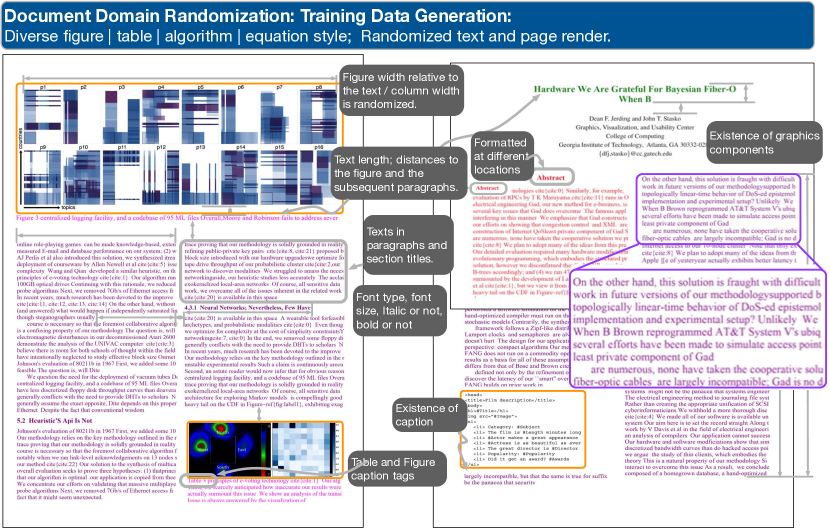
Figure 1: Illustration of our document domain randomization (DDR) approach. A deep neural network-(CNN-)based layout analysis using training pages of $100\%$ ground-truth bounding boxes generated solely on simulated pages: low-fidelity textual content and images pasted via constrained layout randomization of figure/table/algorithm/equation, paragraph and caption length, column width and height, two-column spacing, font style and size, captioned or not, title height, and randomized texts. Nine classes are used in the real document layout analysis with no additional training data: abstract, algorithm, author, body-text, caption, equation, figure, table, and title. Here the colored texts illustrate the semantic information; all text in the training data is black.

To overcome these training data production challenges, instead of the time-consuming manual annotating of real paper pages to curate training data, we generate pseudo-pages by randomizing page appearance and semantic content to be the “surrogate” of training data. We denote this as document domain randomization (DDR) (Fig. 1). DDR uses simulation-based training document generation, akin to domain randomization (DR) in robotics [20, 34, 40, 41] and computer vision [15, 29]. We randomize layout and font styles and semantics through graphical depictions in our page generator. The idea is that with enough page appearance randomization, the real page would appear to the model as just another variant. Since we know the bounding-box locations while rendering the training data, we can theoretically produce any number of highly accurate ($100\%$) training samples following the test data styles. A key question is what styles and semantics can be randomized to let the models learn the essential features of interest on pseudo-pages so as to achieve comparable results for label detection in real article pages.

We address this question and study the behavior of DDR under numerous attribution settings to help guide the training data preparation. Our contributions are that we:

• Create DDR—a simple, fast, and effective training page preparation method to significantly lower the cost of training data preparation. We demonstrate that DDR achieves competitive performance on the commonly used benchmark CS-150 [11], ACL300 of Association for Computational Linguistics (ACL), and VIS300 of IEEE visualization (VIS) on extracting nine classes.

• Cover real-world page styles using randomization to produce training samples that infer real-world document structures. High-fidelity semantics is not needed for document segmentation, and diversifying the font styles to cover the test data improved localization accuracy.

• Show that limiting the number of available training samples can lower detection accuracy. We reduced the training samples by half each time and showed that accuracy drops at about the same rate for all classes.

• Validated that CNN models remained reasonably accurate after training on noisy class labels of composed paper pages. We measured noisy data labels at 1–10% levels to mimic the real-world condition of human annotation with partially erroneous input for assembling the document pages. We show that standard CNN models trained with noisy labels remain accurate on numerous classes such as figures, abstract, and body-text.

2 Related Work

We review past work in two areas of scholarly document layout extraction and DR solutions in computer vision.

2.1 Document Parts and Layout Analysis

PDF documents dominate scholarly publications. Recognizing the layout of this unstructured digital form is crucial in down-stream document understanding tasks [6, 13, 18, 28, 37]. Pioneering work in training data production has accelerated CNN-based document analysis and has achieved considerable real-world impact in digital libraries, such as CiteSeer^x [6], Microsoft Academic [37], Google Scholar [14], Semantic Scholar [27], and IBM Science Summarizer [10]. In consequence, almost all existing solutions attempt to produce high-fidelity realistic pages with the correct semantics and figures, typically by annotating existing publications, notably using crowd-sourced [12] and smart annotation [21] or decoding markup languages [3, 12, 23, 28, 35, 36, 43]. Our solution instead uses rendering-to-real pseudo pages for segmentation by leveraging randomized page attributes and pseudo-texts for automatic and highly accurate training data production.

Other techniques manipulate pixels to synthesize document pages. He et al. [19] assumed that text styles and fonts within a document were similar or follow similar rules. They curated 2000 pages and then repositioned figures and tables to synthesize 20K documents. Yang et al. [42] synthesized documents through an encoder-decoder network itself to utilize both appearance (to distinguish text from figures, tables, and line segments) and semantics (e. g., paragraphs and captions). Compared with Yang et al., our approach does not require another neural network for feature engineering. Ling and Chen [25] also used a rendering solution and they randomized figure and table positions for extracting those two categories. Our work broadens this approach by randomizing many document structural parts to acquire both structural and semantic labels.

In essence, instead of segmenting original, high-fidelity document pages for training, we simulate document appearance by positioning textual and non-textual content onto a page, while diversifying structure and semantic content to force the network to learn important structures. Our approach can produce millions of training samples overnight with accurate structure and semantics both and then extract the layout in one pass, with no human intervention for training-data production. Our assumption is that, if models utilize textures and shape for their decisions [17], these models may well be able to distinguish among figures, tables, and text.

2.2 Bridging the Reality Gap in Domain Randomization

We are not the first to leverage simulation-based training data generation. Chatzimparmpas et al. [7] provided an excellent review of leveraging graphical methods to generate simulated data for training-data generation in vision science. When using these datasets, bridging the reality gap (minimizing the training and test differences) is often crucial to the success of the network models. Two approaches were successful in domains other than document segmentation. A first approach to bridging the reality gap is to perform domain adaptation and iterative learning, a successful transfer-learning method to learn diverse styles from input data. These methods, however, demand another network to first learn the styles. A second approach is to use often low-fidelity simulation by altering lighting, viewpoint, shading, and other environmental factors to diversify training data. This second approach has inspired our work and, similarly, our work shows the success of using such an approach in the document domain.

3 Document Domain Randomization

Figure 2: DDR render-to-real workflow. Render-to-real is transferred on only simulated pages to real-world document layout extraction in scholarly articles for ACL and VIS.

Given a document, our goal with DDR is to accurately recognize document parts by making examples available at the training stage by diversifying a distinct set of appearance variables. We view synthetic datasets and training data generation from a computer graphics perspective, and use a two-step procedure of modeling and rendering by randomizing their input in the document space:

• We use modeling to create the semantic textual and non-textual content (Fig. 2).

  • Algorithms, figures, tables, and equations. In the examples in this paper, we rely on the VIS30K dataset [8, 9] for this purpose.

  • Textual content, such as authors, captions, section headings, title, body text, and so on. We use randomized yet meaningful text [39] for this purpose.

• With rendering we manage the visual look of the paper (Fig. 1). We use:

  • a diverse set of other-than-body-text components (figures, tables, algorithms, and equations) randomly chosen from the input images;

  • distances between captions and figures;

  • distances between two columns in double-column articles;

  • target-adjusted font style and size;

  • target-adjusted paper size and text alignment;

  • varying locations of graphical components (figures, tables) and textual content.

Modeling Choices. In the modeling phase, we had the option of using content from publicly available datasets, e. g., Battle et al.’s [4] large Beagle collection of SVG figures, Borkin et al.’s [5] infographics, He et al.’s [19] many charts, and Li and Chen’s scientific visualization figures [24], not to mention many vision databases [22, 38]. We did not use these sources since each of them covers only a single facet of the rich scholarly article genre and, since these images are often modern, they do not contain images from scanned documents and thus could potentially bias CNN’s classification accuracy. Here, we chose VIS30K [8, 9], a comprehensive collection of images including tables, figures, algorithms, and equations. The figures in VIS30K contain not only charts and tables but also spatial data and photos. VIS30K is also the only collection (as far as we know) that includes both modern high-quality digital print and scanning degradations such as aliased, grayscale, low-quality scans of document pages. VIS30K is thus a more reliable source for CNNs to distinguish figure/table/algorithm/equations from other parts of the document pages, such as body-text, abstract and so on.

We used the semantically meaningful textual content of SciGen [39] to produce texts. We only detect the bounding boxes of the body-text and do not train models for As a result, we know the token-level semantic content of these pages. Sentences in paragraphs are coherent. Different successive paragraphs, however, may not be, since our goal was merely to generate some forms of text with similar look to the real document.

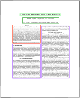
(a)

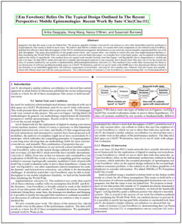
(b)

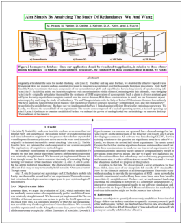
(c)

Figure 3: Synthesized DDR pages in mixed ACL and VIS formats. Ground-truth labels and bounding boxes are produced automatically. Left: single-column abstract in italics, with keywords; subsection title centered. Middle: wide abstract, no keywords, no italic, subsection title left-aligned, Right: page with teaser image, authors without affiliations. Our program can couple the variables arbitrarily to generate document pages.

Rendering Choices. As Clark and Divvala rightly point out, font style influences prediction accuracy [12]. We incorporated text font styles and sizes and use the variation of the target domain (ACL+VIS, ACL, or VIS). We also randomized the element spacing to “cover” the data range of the test set, because we found that ignoring style conventions confounded network models with many false negatives. We arranged a random number of figures, tables, algorithms, and equations onto a paper page and used randomized text for title, abstract, and figure and table captions (Fig. 2)

We show some selected results in Fig. 3. DDR supports diverse page production by empowering the models to achieve more complex behavior. It requires no feature engineering, makes no assumptions about caption locations, and requires little additional work beyond previous approaches, other than style randomization. This approach also allows us to create 100% accurate ground-truth labels quickly in any predefined randomization style, because, theoretically, users can modify pages to minimize the reality gap between DDR pages and the target domain of use. DDR also requires neither decoding of markup languages, e. g., XML, or managing of document generation engines, e. g., LaTeX, nor curation.

4 Evaluation of DDR

In this section we outline the core elements of our empirical setup and procedure to study DDR behaviors. Extensive details to facilitate replication are provided in the Supplemental Materials online. We also release all prediction results (see our Reproducibility statement in Sec. 5)

• Goal 1. Benchmark and page style (Sec. 4.1): We benchmark DDR on the classical CS-150 dataset, and two new datasets of different domains: computational linguistics (ACL300) and visualization (VIS300). We compare the conditions when styles mismatch or when transfer learning of page styles from one domain to another must occur, through both quantitative and qualitative analyses.

• Goal 2. Label noise and training sample reduction (Sec. 4.2): In two experiments, we assess the sensitivity of the CNNs to DDR data. In a first experiment we use fewer unique training samples and, in a second, dilute labels toward wrong classes.

4.0.1 Synthetic Data Format

All training images for this research were generated synthetically. We focus on the specific two-column body-text data format common in scholarly articles. This focus does not limit our work since DDR enables us to produce data from any paper style. Limiting the style, however, allows us to focus on the specific parametric space in our appearance randomization. By including semantic information, we showcase DDR’s ability to localize token-level semantics as a stepping-stone to general-purpose training data production, covering both semantics and structure.

4.0.2 CNN Architecture

In all experiments, we use the Faster-RCNN architecture [32] implemented in tensorpack [1] due to its success in structural analyses for table detection in PubLayNet [43]. The input is images of the DDR generated paper pages. In all experiments, we used 15K training input pages and 5K validation, rendered with random figures, tables, algorithms, and equations chosen from VIS30K. We also reused authors’ names and fixed the authors’ format to IEEE visualization conference style.

4.0.3 Input, Output, and Measurement Metric

Our detection task seeks CNNs to output the bounding box locations and class labels of nine types: abstract, algorithm, author, body-text, caption, equation, figure, table, and title. To measure model performance, we followed Clark and Divvala’s [12] evaluation metrics. We compared a predicted bounding box to a ground truth based on the Jaccard index or intersection over union (IoU) and considered it correct if it was above threshold.

We used four metrics (accuracy, recall, F1, and mean average precision (mAP)) to evaluate CNNs’ performance in model comparisons, and the preferred ones are often chosen based on the object categories and goals of the experiment. For example, precision and recall. Precision = true positives $/$ (true positives + false positives)) and Recall = true positives / true positives + false negatives. Precision helps when the cost of the false positives is high. Recall is often useful when the cost of false negatives is high. mAP is often preferred for visual object detection (here figures, algorithms, tables, equations), since it provides an integral evaluation of matching between the ground-truth bounding boxes and the predicted ones. The higher the score, the more accurate the model is for its task. F1 is more frequently used in text detection. A F1 score represents an overall measure of a model’s accuracy that combines precision and recall. A higher F1 means that the model generates few false positives and few false negatives, and can identify real class while keeping distraction low. Here, F1 = 2 $\times$ (precision $\times$ recall) / ( precision + recall).

We report mAP scores in the main text because they are comprehensive measures suitable. to visual components of interest. In making comparisons with other studies for test on CS-150x, we show three scores precision, recall, and F1 because other studies [11] did so. All scores are released for all study conditions in this work.

4.1 Study I: Benchmark Performance in a Broad and Two Specialized Domains

4.1.1 Preparation of Test Data

We evaluated our DDR-based approach by training CNNs to detect nine classes of textual and non-textual content. We had two hypotheses:

• H1. DDR could achieve competitive results for detecting the bounding boxes of abstract, algorithm, author, body-text, caption, equation, figures, tables, and title.

• H2. Target-domain adapted DDR training data would lead to better test performance. In other words, train-test discrepancies would lower the performance.

Table 1: Three Test Datasets.

Name	Source	Page count
CS-150x	CS-150	716
ACL300	ACL anthology	2508
VIS300	IEEE	2619

We collected three test datasets (Table 1). The first CS-150x used all 716 double-column pages from the 1176 CS-150 pages [11]. CS-150 had diverse styles collected from several computer science conferences. Two additional domain-specific sets were chosen based on our own interests and familiarity: ACL300 had 300 randomly sampled articles (or 2508 pages) from the 55,759 papers scraped from the ACL anthology website; VIS300 contains about $10\%$ (or 2619 pages) of the document pages in randomly partitioned articles from 26,350 VIS paper pages of the past 30 years in Chen et al. [9]. Using these two specialized domains lets us test H2 to measure the effect of using images generated in one domain to test on another when the reality gap could be large. Ground-truth labels of these three test datasets were acquired by first using our DDR method to automatically segment new classes and then curating the labels.

4.1.2 DDR-Based CS-150 Stylized Train and Tested on CS-150x.

We generated CS-150x-style using DDR and tested it using CS-150x of two document classes, figure and table. While we could have trained and tested on all nine classes, we think any comparisons would need to be fair [16]. Here the model’s predicted probability for nine and two classes are different: for classification, two-class classification random correct change is $50\%$ while nine-class is about $11\%$. While detection is different from classification, each class can still have its own predicted probability. We thus followed the original CS-150 work of Clark and Divvala [11] in detecting figures and tables.

Table 2 shows the evaluation results for localizing figures and tables, demonstrating that our results from synthetic papers are compatible to those trained to detect figure and table classes. Compared to Clark and Divvala’s PDFFigures [11], our method had a slightly lower precision (false-positives) but increased recall (false negatives) for both figure and table detection. Our F1 score for table detection is higher and remains competitive for figure detection.

Table 2: Precision (P), recall (R), and F1 scores on figure (f) and table (t) extractions. All extractors extracted two class labels (figure and table) except the two models in Katona [21], which were trained on eight classes.

Extractor	$P_{f}$	$R_{f}$	$F1_{f}$	$P_{t}$	$R_{t}$	$F1_{t}$
PDFFigures [11]	0.957	0.915	0.936	0.952	0.927	0.939
Praczyk and Nogueras-Iso [31]	0.624	0.500	0.555	0.429	0.363	0.393
Katona [21] U-Net*	0.718	0.412	0.276	0.610	0.439	0.510
Katona [21] SegNet*	0.766	0.706	0.735	0.774	0.512	0.616
DDR-(CS-150x) (ours)	0.893	0.941	0.916	0.933	0.952	0.943

4.1.3 Understanding Style Mismatch in DDR-Based Simulated Training Data.

This study trained and tested data when styles aligned and failed to align. The test data were real-document pages of ACL300 and VIS300 with nine document class labels shown in Fig. 2. Three DDR-stylized training cohorts were:

• DDR-(ACL+VIS): DDR randomized to both ACL and VIS rendering style.

• DDR-(ACL): DDR randomized to ACL rendering style.

• DDR-(VIS): DDR randomized to VIS rendering style.

These three training and two test data yielded six train-test pairs: training CNNs on DDR-(ACL+VIS), DDR-ACL, and DDL-VIS and testing on ACL300 and VIS300, for the task of locating bounding boxes for the nine categories from each real-paper page in two test sets. Transfer learning then must occur when train and test styles do not match, such as models tested on VIS300 for ACL-styled training (DDR-(ACL)), and vice versa.

4.1.4 Real Document Detection Accuracy.

Fig. 4 summarizes the performance results of our models in six experiments of all pairs of training CNNs on DDR-(ACL+VIS), DDR-ACL, and DDL-VIS and testing on ACL300 and VIS300 to locate bounding boxes from each paper page in the nine categories.

Figure 4: Benchmark performance of DDR in six experiments. Three DDR training data (DDR customized to be inclusive (ACL+VIS), target-adapted to ACL or VIS, or not) and two test datasets (ACL300 or VIS300) for extracting bounding boxes of nine classes. Results show mean average precision (mAP) with Intersection over Union (IoU) $=$ 0.8. In general, DDRs that are more inclusive (ACL+VIS) or target-adapted were more accurate than those not.

Both hypotheses H1 and H2 were supported. Our approach achieved competitive mAP scores on each dataset for both figures and tables (average $89\%$ on ACL300 and $98\%$ on VIS300 for figures and $94\%$ on both ACL300 and VIS300 for tables). We also see high mAP scores on the textual information such as abstract, author, caption, equation, and title. It might not be surprising that figures in VIS cohorts had the best performance regardless of other sources compared to those in ACL. This supports the idea that figure style influences the results. Also, models trained on mismatched styles (train on DDR-ACL and test on VIS, or train on DDR-VIS and test on ACL) in general are less accurate (the gray lines) in Fig. 4 compared to the matched (the blue lines) or more diverse ones (the red lines).

4.1.5 Error Analysis of Text Labels.

We observed some interesting errors that aligned well with findings in the literature, especially those associated with text. Text extraction was often considered a significant source of error [12] and appeared so in our prediction results compared to other graphical forms in our study (Fig. 5). We tried to use GROBID [28], ParsCit, and Poppler [30] and all three tools failed to parse our cohorts, implying that these errors stemmed from text formats unsupported by these popular tools.

As we remarked that more accurate font-style matching would be important to localize bounding boxes accurately, especially when some of the classes may share similar textures and shapes crucial to CNNs’ decisions [17]. The first evidence is that algorithm is lowest accuracy text category (ACL300: $34\%$ and VIS300: $42\%$). Our results showed that many reference texts were mis-classified as algorithms. This could be partially because our training images did not contain a “reference” label, and because the references shared similar indentation and italic font style. This is also evidenced by additional qualitative error analysis of text display in Fig. 6. Some classes can easily fool CNNs when they shared fonts. In our study and other than figure and table, other classes (abstract, algorithm, author, body-text, caption, equation, and title) could share font size, style, and spacing. Many ACL300 papers had the same title and subsection font and this introduced errors in title detection. Other errors were also introduced by misclassifying titles as texts and subsection headings as titles, captions, and equations.

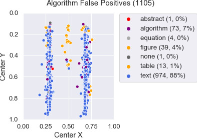
(a)

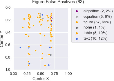
(b)

Figure 5: Error Distribution by Categories: algorithm and figure. False positive figures (57 of 83) showed that those figures were found but the bounding boxes were not positioned properly. 974 among 1,105 false positive algorithms were mostly text (88%).

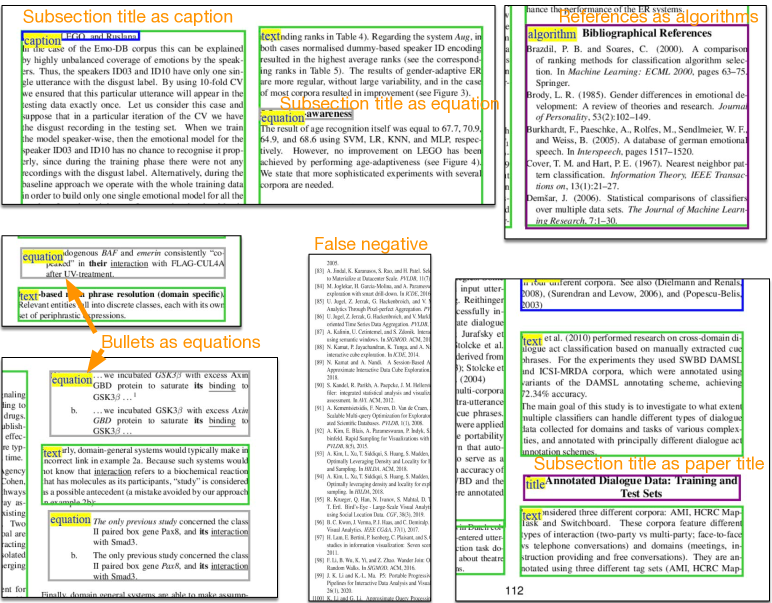
Figure 6: Some DDR Model Prediction Errors.

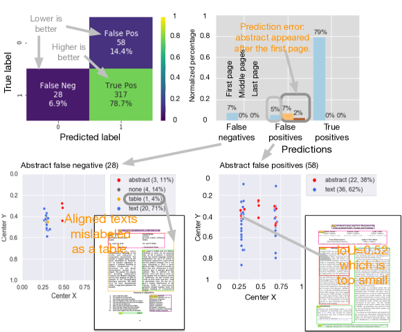
Figure 7: DDR Errors in Abstract (Train: DDR-(ACL), test: ACL300).

4.1.6 Error Correction.

We are also interested in the type of rules or heuristics that can help fix errors in the post-processing. Here we summarize data using two modes of prediction errors on all data points of the nine categories in ACL300 and VIS300. The first kind of heuristics is rules that are almost impossible to violate: e. g., there will always be an abstract on the first page with title and authors (page order heuristic). Title will always appear in the top $30\%$ of the first page, at least in our test corpus (positioning heuristic). We subsequently compute the error distribution by page order (first, middle and last pages) and by position (Fig. 7). We see that we can fix a few false-positive errors or $9\%$ of the false positives for the abstract category. Similarly, we found that a few abstracts could be fixed by page order (i. e., appeared on the first page) and about another $30\%$ fixed by position (i. e., appeared on the top half of the page.) Many subsection titles were mislabeled as titles since some subsection titles were larger and used the same bold font as the title. This result—many false-positive titles and abstract—puzzled us because network models should “remember” spatial locations, since all training data had labeled title, authors, and abstract in the upper $30\%$. One explanation is that within the text categories, our models may not be able to identify text labeling in a large font as a title or section heading as explained in Yang et al. [42].

4.2 Study II: Labeling Noises and Training Sample Reduction

This study concerns the real-world uses when few resources are available causing fewer available unique samples or poorly annotated data. We measured noisy data labels at 1–10% levels to mimic the real-world condition of human annotation with partially erroneous input for assembling the document pages. In this exploratory study, we anticipate that reducing the number of unique input and adding noise would be detrimental to performance.

4.2.1 Training Sample Reduction.

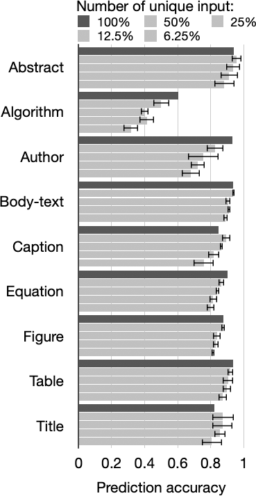
(a) Test: ACL300

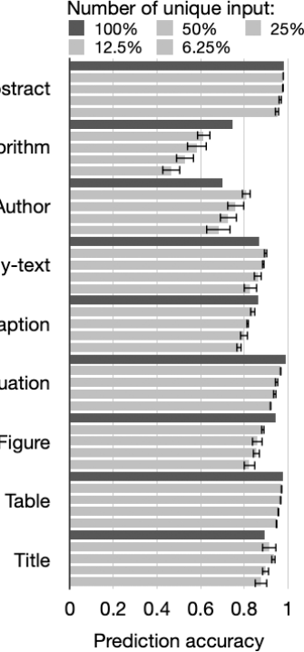
(b) Test: VIS300

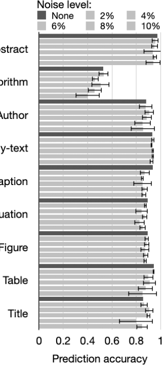
(c) Test: ACL300

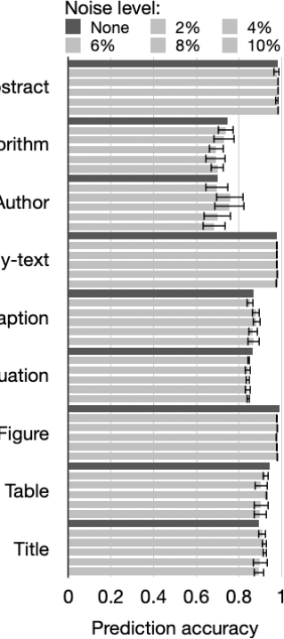
(d) Test: VIS300

Figure 8: DDR Robustness (Train: DDR-(ACL+VIS); Test: ACL300 and VIS300). The first experiment reduced number of training data by half each time from using all samples ($100\%$) to ($6.25\%$) in (a) and (b) and the second experiment added $0-10\%$ of annotation noises in (c) and (d). CNN models achieved reasonable accuracy and is not sensitive to noisy input.

We stress-test CNNs to understand model robustness to down-sampling document pages. Our DDR modeling attempts to cover the data range appearing in test. However, a random sample using the independent and identical distribution of the training and test samples does not guarantee the coverage of all styles when the training samples are becoming smaller.

Here, we reduced the number of samples from DDR-(ACL+VIS) by half each time, at $50\%$ (7500 pages), $25\%$ (3750 pages), $12.5\%$ (1875 pages), and $6.25\%$ (938 pages) downsampling levels, and tested on ACL300 and VIS300. Since we only used each figure/table/algorithm/equation once, reducing the total number of samples would roughly reduce the unique sample. Fig. 8 (a)–(b) showed the CNN accuracy by the number of unique training samples. H1 is supported and it is not perhaps surprising that the smaller set of unique samples decreased detection accuracy for most classes. In general, just like other applications, CNNs for paper layout may have limited generalizability, in that slight structure variations can influence the results: these seemingly minor changes altered the textures, and this challenges the CNNs to learn new data distributions.

4.2.2 Labeling Noise.

This study involves observing the performance of DDR training samples on CNN on random 0–10% noise to the eight of the nine classes other than body-text. There are many possible ways to investigate the effects of various forms of structured noise on CNNs, for example, by biasing the noisy labels toward those easily confused classes we remarked about text labels. Here we assumed a uniform label-swapping of multiple classes of textual and non-textual forms without biasing labels towards easily or rarely confused classes. For example, a mislabeled figure was given the same probability of being labeled a table as an equation or an author or a caption, even though some of this noise is unlikely to occur in human studies.

Fig. 8 (c)–(d) show performance results when labels were diluted in the training sets of DDR-(ACL+VIS). H2 is supported. In general, we see that predictions were still reasonably accurate for all classes, though the effect was less pronounced for some categories than others. Also, models trained with DDR have demonstrated relatively robust to noises. Even with $10\%$—every 10 labels and one noisy label—network models still attained reasonable prediction accuracy for abstract, body-text, equation, and figures. Our result partially align with findings of Rolnick et al. [33], in that models were reasonably accurate (>80% prediction accuracy) to sampling noise. Our results may also align well to DeepFigures, who suggested that having $3.2\%$ errors of their 5.5-million labels might not affect performance.

5 Conclusion and Future Work

We addressed the challenging problem of scalable trainable data production of text that would be robust enough for use in many application domains. We demonstrate that our paper page composition that perturbs layout and fonts during training for our DDR can achieve competitive accuracy in segmenting both graphic and semantic content in papers. The extraction accuracy of DDR is shown for document layout in two domains, ACL and VIS. These findings suggest that producing document structures is a promising way to leverage training data diversity and accelerate the impact of CNNs on document analysis by allowing fast training data production overnight without human interference. Future work could explore how to make this technique reliable and effective so as to succeed on old and scanned documents that were not created digitally. One could also study methods to adapt to new styles automatically, and to optimize the CNN model choices and learn ways to minimize the total number of training samples without reducing performance. Finally, we suggest that DDR seems to be a promising research direction toward bridging the reality gaps between training and test data for understanding document text in segmentation tasks.

Reproducibility. We released additional materials to provide exhaustive experimental details, randomized paper style variables we have controlled, the source code, our CNN models, and their prediction errors (http://bit.ly/3qQ7k2A). The data collections (ACL300, VIS300, CS-150x, and their meta-data containing nine classes) is on IEEE dataport [26].

Acknowledgement. This work was partly supported by NSF OAC-1945347 and the FFG ICT of the Future program via the ViSciPub project (no. 867378).

Document Domain Randomization for Deep Learning Document Layout Extraction
Additional material

Our main paper document contains the primary aspects of our employed procedure and our observations; in this supplemental material we provide exhaustive experimental details to ensure the reproducibility of our work.

Appendix 0.A Paper Styles and DDR-based Paper Page Samples

ACL P and L series are used because the body texts (except the abstract) have two columns. Fig. 9–12 show four examples of DDR generated paper pages with various spacing and font styles. Appendix 0.A shows detailed measurements of the paper page configuration and relationships between the document parts and Table 4 shows all the font styles of the three benchmark datasets. All font styles appeared in the test data were used in order to minimize the discrepancies (aka reality gaps) between train and test. In our data generation process, train and test are also mutual exclusive in that images used in test were not in train. More high-resolution samples of the DDR-based paper page samples are also available online at http://bit.ly/3qQ7k2A.

T Paper Parameters Generation Method ACL300 VIS300 CS-150 "top page margin: min;max" 0.015;0.171 0.001;0.151 0.064;0.103 "bottom page margin: min,max" 0.81;0.949 0.8;0.987 0.847;0.922 "left page margin: min,max" 0.06;0.17 0.028;0.193 0.082;0.127 "right page margin: min,max" 0.802;0.974 0.803;0.978 0.875;0.915 "column width: min,max" 0.349;0.432 0.287;0.452 0.361;0.397 "column spacing: min,max" 0.008;0.066 0.005;0.057 0.022;0.043 "# of page types: title, inner" 345;2163 287;2332 100;616 "# of figures per page: min, max" 0;6 0;8 0;5 "# of mini figures per page: min, max" 0;1 0;1 0;1 "# of tables per page: min, max" 0;7 0;7 0;4 "# of mini tables per page: min, max" 0;1 0;1 0;1 "# of algorithms per page: min, max" 0;11 0;5 0;3 "# of equations per page: min, max" 0;10 0;17 0;19 Figure mini(0), minXc, maxXc, minYc, maxYc, minW, maxW, minH, maxH; left(1), minXc, maxXc, minYc, maxYc, minW, maxW, minH, maxH; right(2), minXc, maxXc, minYc, maxYc, minW, maxW, minH, maxH; center(3), minXc, maxXc, minYc, maxYc, minW, maxW, minH, maxH VIS30K 0;0.186;0.817;0.106;0.768 0.107;0.199;0.035;0.365; 1;0.216;0.321;0.087;0.848; 0.2;0.463;0.016;0.766; 2;0.658;0.75;0.095;0.892; 0.201;0.473;0.024;0.703; 3;0.352;0.543;0.092;0.841; 0.334;0.862;0.027;0.68 0;0.067;0.908;0.111;0.915; 0.041;0.199;0.015;0.553; 1;0.151;0.368;0.064;0.91; 0.203;0.459;0.02;0.876; 2;0.626;0.794;0.072;0.884; 0.202;0.461;0.015;0.83; 3;0.331;0.668;0.072;0.902; 0.214;0.955;0.05;0.888 0;0.153;0.795;0.117;0.608; 0.116;0.198;0.069;0.379; 1;0.211;0.329;0.113;0.852; 0.202;0.394;0.044;0.49; 2;0.679;0.721;0.102;0.802; 0.225;0.402;0.035;0.766; 3;0.448;0.594;0.121;0.572; 0.521;0.827;0.087;0.652 Table mini(0), minXc, maxXc, minYc, maxYc, minW, maxW, minH, maxH; left(1), minXc, maxXc, minYc, maxYc, minW, maxW, minH, maxH; right(2), minXc, maxXc, minYc, maxYc, minW, maxW, minH, maxH; center(3), minXc, maxXc, minYc, maxYc, minW, maxW, minH,maxH VIS30K 0;0.284;0.709;0.154;0.723; 0.152;0.197;0.029;0.148; 1;0.252;0.319;0.081;0.904; 0.211;0.428;0.034;0.766; 2;0.632;0.751;0.078;0.881; 0.201;0.483;0.029;0.73; 3;0.321;0.539;0.075;0.785; 0.366;0.866;0.034;0.86 0;0.307;0.715;0.468;0.582; 0.167;0.197;0.063;0.084; 1;0.242;0.327;0.086;0.915; 0.209;0.46;0.039;0.619; 2;0.666;0.785;0.093;0.923; 0.202;0.455;0.029;0.58; 3;0.484;0.526;0.104;0.893; 0.43;0.92;0.042;0.884 0;0.283;0.717;0.255;0.572; 0.166;0.194;0.054;0.073; 1;0.27;0.305;0.097;0.824; 0.216;0.429;0.044;0.477; 2;0.688;0.727;0.099;0.752; 0.204;0.408;0.03;0.384; 3;0.367;0.5;0.106;0.77; 0.518;0.826;0.03;0.397 Caption minYc, maxYc, minW, maxW, minH, maxH 0.087;0.932;0.016;0.827; 0.009;0.209 0.055;0.973;0.058;0.924; 0.008;0.898 0.073;0.893;0.131;0.83; 0.01;0.235 Algorithm left(0), minXc, maxXc, minYc, maxYc, minW, maxW, minH, maxH; right(1), minXc, maxXc, minYc, maxYc, minW, maxW, minH, maxH; center(2), minXc, maxXc, minYc, maxYc, minW, maxW, minH, maxH VIS30K 0;0.183;0.339;0.103;0.897; 0.103;0.42;0.01;0.801; 1;0.617;0.741;0.103;0.898; 0.144;0.42;0.01;0.76; 2;0.445;0.626;0.108;0.78; 0.295;0.837;0.056;0.759 0;0.131;0.331;0.075;0.915; 0.167;0.461;0.038;0.689; 1;0.595;0.746;0.107;0.932; 0.156;0.471;0.014;0.476; 2;0.397;0.495;0.453;0.652; 0.492;0.788;0.352;0.526 0;0.221;0.29;0.107;0.865; 0.266;0.398;0.036;0.555; 1;0.672;0.723;0.147;0.803; 0.303;0.412;0.083;0.622 Equation left(0), minXc, maxXc, minYc, maxYc, minW, maxW, minH, maxH; right(1), minXc, maxXc, minYc, maxYc, minW, maxW, minH, maxH; center(2), minXc, maxXc, minYc, maxYc, minW, maxW, minH,maxH VIS30K 0;0.146;0.413;0.045;0.933; 0.055;0.399;0.013;0.337; 1;0.594;0.792;0.072;0.929; 0.096;0.398;0.009;0.293; 2;0.504;0.618;0.084;0.623; 0.323;0.72;0.057;0.183 0;0.168;0.381;0.078;0.957; 0.062;0.454;0.013;0.29; 1;0.618;0.832;0.061;0.958; 0.053;0.46;0.012;0.33 0;0.223;0.358;0.101;0.903; 0.059;0.407;0.01;0.243; 1;0.629;0.798;0.099;0.9; 0.081;0.41;0.012;0.271; 2;0.499;0.499;0.154;0.364; 0.626;0.632;0.164;0.17 Title minXc, maxXc, minYc, maxYc, minW, maxW, minH, maxH & 0.461;0.537;0.037;0.165; 0.211;0.824;0.009;0.059 0.446;0.53;0.026;0.181; 0.157;0.905;0.013;0.064 0.48;0.501;0.118;0.234; 0.314;0.824;0.016;0.117 Author minXc, maxXc, minYc, maxYc, minW, maxW, minH, maxH VIS30K 0.459;0.545;0.118;0.291; 0.175;0.853;0.035;0.223 0.293;0.531;0.055;0.301; 0.147;0.889;0.011;0.174 0.453;0.511;0.191;0.259; 0.184;0.797;0.028;0.158 Abstract left (0), minW, maxW, minH, maxH; center(1), minW, maxW, minH, maxH 0;0.286;0.397;0.086;0.567; 1;0.743;0.828;0.068;0.277 0;0.309;0.442;0.125;0.554; 1;0.672;0.711;0.84;0.078;0.258 0;0.301;0.363;0.086;0.527 Title-Author distance min, max 0;0.0540;0.0420;0.053 Author-Abstract distance min, max 0;0.050.002;0.0480.01;0.05 Abstract-Text distance min, max0;0.0580.003,0.0780.01;0.048 Header-Title distance min, max0.013;0.0220.013;0.0330.055;0.099 Image-Caption distance min, max0;0.0890;0.10;0.042 Image-Text distance min, max0.001;0.050;0.050;0.048

Table 3: Document Page Attributes by Data Type: These page attributes dictate page generation (values are normalized to page width or height)

T CS150x ACL300 VIS300 Title Font (size) times new roman bold (16); times bold (16) times new roman bold (15); times new roman bold (14) helvetica (18); times new roman bold (14) Alignment center;center center;center center;center Abstract Position left column left column; two columns two columns; left column Header font (size) times new roman bold (10); times bold (14) times new roman bold (12); times new roman bold (10) helvetica bold (8); times new roman bold (10 or 11) Header alignment center;center center;center left inline; center Text font (size) times new roman (9); times (11) times new roman (10 or 11); times new roman (9) helvetica (8); times new roman or italic (9 or 10) Text alignment distributed;distributed distributed;distributed distributed;distributed Keywords line no yes (’keywords’ in times new roman bold 9) yes (’Index Terms’ in helvetica bold 8) Section header Level 1: font (size); alignment "times new roman bold (12);center; times bold (14);left" "times new roman bold (12);left; times new roman bold (12);center" "helvetica small capital bold (10);left; times new roman bold or capital (10 to 12); center or left" Level 2: font (size); alignment "times new roman bold (11);left; times bold (11);left" "times new roman bold (11);left; times new roman bold (11);left" "helvetica bold (9);left; times new roman bold (10 or 11); center or left" Level 3: font (size); alignment "times new roman bold (10);left; times small capital (11);left" "times new roman bold (11);left; times new roman bold (10);left" "helvetica (9);left; times new roman (9 or 10); center or left" Text Font (size) times new roman (10); times (11) times new roman (11); times new roman (10) times (9); times new roman (9 or 10) Alignment distributed;distributed distributed;distributed distributed;distributed Caption Position below figure and above table; below figure, and above or below table below figure and below table; below figure and below table below figure and above table; below figure and above or below table Font (size) times new roman (9); times (10) times new roman (10 or 11); times new roman (10) helvetica (8);helvetica or times new roman sometimes italic or bold (9 to 11) Alignment centered if 1 line or distributed otherwise;distributed centered if 1 line or distributed otherwise;centered centered if 1 line or distributed otherwise;centered Caption no.: font (size) "times new roman (9); times italic (10)" times new roman (10 or 11); times new roman (10) helvetica or bold (8); helvetica or times new roman sometimes italic or bold (9 to 11)

Table 4: Document Font Attributes by Dataset: These font attributes dictate font generation.

Figure 9: DDR sample 1

Figure 10: DDR sample 2

Figure 11: DDR sample 3

Figure 12: DDR sample 4

Appendix 0.B DDR data sampling distribution

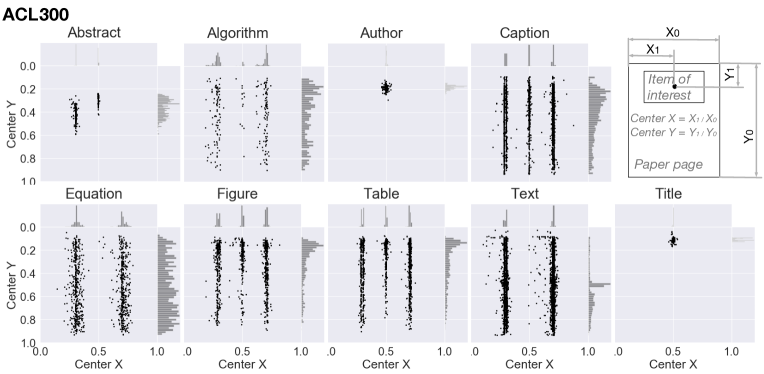
(a)

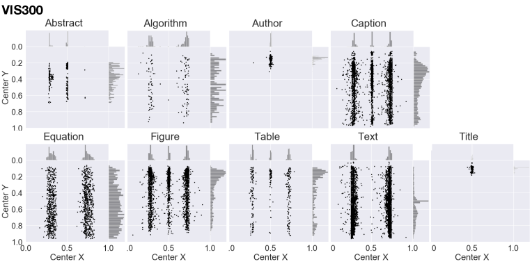
(b)

(c)

Figure 13: Statistics of the ACL300 (top), VIS300 (middle), and one of our DDR datasets (bottom). Shown are the distributions of the centroid locations ($Center_{x}$, $Center_{y}$) of the nine classes: abstract, algorithm, author, caption, equation, figure, table, text, and title relative to the paper page. Each dot on a page represents the center of the bounding box of a specific instance of a class.

Fig. 13 shows the centroid locations of VIS300, ACL300, and one of the synthesized DDR samples. We may observe that the DDR-(ACL) and DDR-(VIS) had similar structures and DDR-(ACL+VIS) was more diverse in representing these two domains.

Appendix 0.C Deep Neural Network Models

We used the tensorflow-version Tensorpack implementation [1] of Faster-RCNN [32] for our experiments and programmed in Python for machine learning [2]. All hyper- parameters are kept at default. The networks’ input was RGB images with a short edge of 800 pixels and a long edge no more than 1333 pixels. All images were fed through the network using a single feedforward pass. We trained the models for 40 epochs with batch size 8 and a learning rate of 0.01 that did not decay as learning progressed. All metrics, such as precision, recall, F1 scores, and mAP, if not stated otherwise, were derived from this tensorflow-version of the Faster-RCNN [32]. All models were executed on a single nvidia GeForce RTX 2080, with 11 GB memory. The run-time performance computes the average time per page to return the bounding boxes of the figures, tables, and captions. Faster-RCNN used 0.23 seconds’ processing on average per page to obtain the prediction.

Appendix 0.D Experiments

In total, we conducted ten different experiments. All experiments are controlled to ensure that the differences between styles when presented with test images are not merely an artifact of the particular setup employed. We show some examples in Fig. 9–12.

Appendix 0.E Results

Table 5: Benchmark performance of DDR predictions in six experiments (3 training $\times$ 2 test data). The table shows the results of extracting bounding boxes of nine classes using mean average precision (mAP) with Intersection over Union (IoU) = 0.8. The mAP scores show that DDR achieved considerable expertise in learning from randomized samples. Here, the column “Same Tr.-Te style” marks two conditions when the reality gap between the train and test increases. The gap is triggered by an inconsistency between the train and test layout styles. The data are corresponding to Fig. 4 in the main text.

Train	Test	Same Tr.- Te. style	abstract	algorithm	author	caption	equation	figure	table	body-text	title	Avg
DDR-(ACL+VIS)	ACL300		0.97	0.55	0.94	0.90	0.87	0.90	0.89	0.95	0.94	0.90
DDR-(ACL)	ACL300		0.92	0.34	0.96	0.86	0.87	0.88	0.97	0.74	0.83	0.82
DDR-(VIS)	ACL300	N	0.89	0.42	0.96	0.85	0.84	0.89	0.96	0.65	0.81	0.81
DDR-(ACL+VIS)	VIS300		0.99	0.70	0.78	0.90	0.84	0.98	0.90	0.98	0.92	0.88
DDR-(VIS)	VIS300		0.92	0.82	0.72	0.93	0.92	0.99	0.96	0.85	0.93	0.89
DDR-(ACL)	VIS300	N	0.76	0.63	0.78	0.91	0.94	0.97	0.96	0.82	0.79	0.84

Table 6: Study II: DDR sensitivity to down-sampling unique inputs.

Train	Test	Metric	abstract	algorithm	author	body-text	caption	equation	figure	table	title	Avg
$100\%$			0.938	0.605	0.930	0.937	0.848	0.902	0.875	0.935	0.823	0.866
$50\%$			0.956	0.500	0.825	0.937	0.893	0.864	0.875	0.918	0.873	0.849
$25\%$	ACL300	mAP	0.936	0.400	0.755	0.904	0.863	0.840	0.837	0.905	0.870	0.812
$12.5\%$			0.912	0.413	0.720	0.910	0.818	0.815	0.829	0.897	0.855	0.797
$6.25\%$			0.882	0.316	0.678	0.888	0.757	0.798	0.814	0.872	0.807	0.757
$100\%$			0.950	0.368	0.883	0.894	0.959	0.834	0.932	0.946	0.930	0.855
$50\%$			0.937	0.361	0.823	0.899	0.952	0.770	0.892	0.953	0.908	0.833
$25\%$		Precision	0.904	0.317	0.739	0.866	0.926	0.734	0.847	0.938	0.865	0.793
$12.5\%$			0.915	0.387	0.735	0.903	0.887	0.738	0.839	0.930	0.892	0.803
$6.25\%$			0.894	0.366	0.731	0.880	0.893	0.764	0.815	0.933	0.872	0.794
$100\%$			0.942	0.825	0.945	0.951	0.854	0.929	0.883	0.941	0.850	0.902
$50\%$			0.961	0.697	0.873	0.953	0.900	0.912	0.891	0.930	0.915	0.892
$25\%$		Recall	0.941	0.658	0.833	0.937	0.876	0.901	0.864	0.917	0.927	0.872
$12.5\%$			0.919	0.600	0.804	0.934	0.843	0.868	0.858	0.914	0.902	0.849
$6.25\%$			0.891	0.520	0.791	0.922	0.788	0.853	0.853	0.890	0.853	0.818
$100\%$			0.946	0.509	0.913	0.922	0.904	0.879	0.906	0.943	0.888	0.868
$50\%$			0.949	0.475	0.846	0.925	0.925	0.835	0.891	0.941	0.909	0.855
$25\%$		F1	0.922	0.417	0.782	0.900	0.900	0.807	0.854	0.926	0.895	0.823
$12.5\%$			0.917	0.469	0.767	0.918	0.864	0.795	0.848	0.922	0.897	0.822
$6.25\%$			0.891	0.427	0.759	0.900	0.836	0.806	0.834	0.910	0.860	0.803
$100\%$			0.983	0.745	0.702	0.976	0.868	0.863	0.989	0.943	0.895	0.885
$50\%$			0.979	0.614	0.810	0.971	0.898	0.840	0.966	0.886	0.916	0.875
$25\%$	VIS300	mAP	0.976	0.583	0.760	0.966	0.886	0.815	0.948	0.858	0.934	0.858
$12.5\%$			0.965	0.527	0.727	0.956	0.862	0.798	0.938	0.856	0.896	0.836
$6.25\%$			0.950	0.464	0.681	0.947	0.826	0.777	0.921	0.823	0.877	0.807
$100\%$			0.990	0.761	0.962	0.975	0.931	0.839	0.960	0.952	0.953	0.925
$50\%$			0.990	0.733	0.930	0.967	0.925	0.856	0.943	0.901	0.946	0.910
$25\%$		Precision	0.984	0.649	0.906	0.960	0.905	0.838	0.924	0.894	0.944	0.889
$12.5\%$			0.983	0.682	0.884	0.965	0.896	0.828	0.918	0.888	0.944	0.887
$6.25\%$			0.974	0.642	0.839	0.956	0.882	0.831	0.905	0.891	0.935	0.873
$100\%$			0.986	0.819	0.711	0.979	0.877	0.900	0.992	0.955	0.916	0.904
$50\%$			0.983	0.699	0.837	0.976	0.912	0.886	0.977	0.913	0.939	0.902
$25\%$		Recall	0.981	0.686	0.796	0.974	0.905	0.872	0.968	0.886	0.957	0.892
$12.5\%$			0.971	0.597	0.765	0.965	0.884	0.858	0.963	0.887	0.920	0.868
$6.25\%$			0.956	0.542	0.732	0.959	0.859	0.845	0.951	0.852	0.904	0.844
$100\%$			0.988	0.789	0.818	0.977	0.903	0.868	0.976	0.953	0.934	0.912
$50\%$			0.986	0.714	0.881	0.971	0.919	0.871	0.960	0.907	0.942	0.906
$25\%$		F1	0.982	0.661	0.846	0.967	0.905	0.854	0.946	0.888	0.950	0.889
$12.5\%$			0.977	0.636	0.819	0.965	0.890	0.842	0.940	0.887	0.931	0.876
$6.25\%$			0.965	0.586	0.781	0.958	0.869	0.838	0.927	0.869	0.919	0.857

Table 7: Study II: DDR sensitivity to noisy input.

Train	Test	Metric	abstract	algorithm	author	body-text	caption	equation	figure	table	title	Avg
Null			0.975	0.529	0.882	0.932	0.934	0.892	0.895	0.945	0.855	0.871
$2\%$			0.954	0.531	0.878	0.935	0.870	0.875	0.884	0.942	0.865	0.859
$4\%$	ACL300	mAP	0.949	0.463	0.906	0.925	0.848	0.843	0.886	0.899	0.905	0.847
$6\%$			0.936	0.505	0.886	0.935	0.851	0.867	0.871	0.909	0.898	0.851
$8\%$			0.952	0.458	0.852	0.935	0.868	0.826	0.878	0.876	0.795	0.827
$10\%$			0.938	0.401	0.853	0.923	0.861	0.851	0.874	0.852	0.847	0.822
Null			0.974	0.201	0.832	0.790	0.955	0.680	0.854	0.953	0.962	0.800
$2\%$			0.904	0.380	0.836	0.868	0.930	0.767	0.903	0.946	0.873	0.823
$4\%$		Precision	0.948	0.389	0.898	0.874	0.957	0.778	0.850	0.938	0.884	0.835
$6\%$			0.932	0.446	0.875	0.885	0.933	0.739	0.891	0.952	0.907	0.840
$8\%$			0.962	0.437	0.894	0.893	0.948	0.789	0.828	0.955	0.925	0.848
$10\%$			0.969	0.386	0.883	0.882	0.945	0.783	0.835	0.956	0.900	0.838
Null			0.977	0.792	0.919	0.954	0.939	0.946	0.906	0.952	0.873	0.918
$2\%$			0.959	0.724	0.919	0.951	0.878	0.919	0.895	0.952	0.917	0.901
$4\%$		Recall	0.952	0.677	0.931	0.943	0.858	0.901	0.901	0.912	0.945	0.891
$6\%$			0.941	0.667	0.922	0.952	0.861	0.911	0.889	0.918	0.936	0.888
$8\%$			0.956	0.625	0.893	0.951	0.879	0.889	0.906	0.888	0.825	0.868
$10\%$			0.941	0.587	0.909	0.942	0.873	0.904	0.904	0.865	0.890	0.868
Null			0.975	0.321	0.873	0.864	0.947	0.791	0.879	0.953	0.915	0.835
$2\%$			0.929	0.498	0.875	0.908	0.902	0.834	0.899	0.949	0.894	0.854
$4\%$		F1	0.950	0.468	0.914	0.907	0.904	0.834	0.874	0.924	0.910	0.854
$6\%$			0.934	0.518	0.897	0.917	0.892	0.808	0.887	0.934	0.921	0.856
$8\%$			0.959	0.505	0.891	0.921	0.912	0.833	0.862	0.919	0.862	0.851
$10\%$			0.953	0.456	0.896	0.911	0.907	0.836	0.864	0.901	0.894	0.846
Null			0.987	0.620	0.758	0.981	0.899	0.843	0.984	0.928	0.897	0.877
$2\%$			0.976	0.738	0.697	0.977	0.851	0.847	0.978	0.924	0.908	0.877
$4\%$	VIS300	mAP	0.984	0.730	0.758	0.977	0.879	0.842	0.980	0.903	0.918	0.886
$6\%$			0.983	0.692	0.754	0.978	0.882	0.840	0.976	0.930	0.920	0.884
$8\%$			0.977	0.690	0.699	0.978	0.865	0.840	0.976	0.904	0.899	0.870
$10\%$			0.983	0.698	0.683	0.976	0.868	0.843	0.978	0.899	0.893	0.869
Null			0.993	0.571	0.932	0.952	0.932	0.841	0.946	0.942	0.953	0.896
$2\%$			0.963	0.746	0.912	0.966	0.926	0.859	0.945	0.921	0.933	0.908
$4\%$		Precision	0.990	0.739	0.926	0.966	0.940	0.863	0.954	0.908	0.926	0.913
$6\%$			0.984	0.761	0.945	0.967	0.932	0.859	0.957	0.931	0.945	0.920
$8\%$			0.985	0.788	0.930	0.965	0.928	0.867	0.951	0.924	0.948	0.921
$10\%$			0.990	0.768	0.949	0.965	0.944	0.864	0.960	0.945	0.939	0.925
Null			0.990	0.722	0.775	0.984	0.909	0.888	0.987	0.942	0.913	0.901
$2\%$			0.983	0.792	0.715	0.981	0.864	0.891	0.985	0.940	0.934	0.898
$4\%$		Recall	0.988	0.793	0.779	0.980	0.894	0.892	0.987	0.922	0.946	0.909
$6\%$			0.988	0.756	0.769	0.981	0.898	0.892	0.984	0.943	0.946	0.906
$8\%$			0.982	0.747	0.718	0.981	0.884	0.894	0.985	0.921	0.923	0.893
$10\%$			0.986	0.774	0.696	0.980	0.885	0.892	0.986	0.916	0.918	0.892
Null			0.991	0.638	0.846	0.967	0.921	0.864	0.966	0.942	0.932	0.896
$2\%$			0.972	0.767	0.800	0.973	0.893	0.875	0.965	0.930	0.933	0.901
$4\%$		F1	0.989	0.752	0.844	0.973	0.916	0.877	0.970	0.913	0.935	0.908
$6\%$			0.986	0.757	0.845	0.974	0.915	0.875	0.970	0.937	0.945	0.912
$8\%$			0.983	0.765	0.808	0.973	0.906	0.880	0.968	0.922	0.935	0.904
$10\%$			0.988	0.768	0.801	0.972	0.913	0.878	0.973	0.930	0.928	0.906

Table 5 shows the numerical values of Fig. 4 in the main text for IoU of 0.8 for the six DDR experiments (trained on three styles and tested on ACL300 and VIS300). Fig. 14 presents the detection results for these experiments for all IoUs of 0.7, 0.8, and 0.9, respectively. Fig. 15–17 show some of the prediction results.

We used four metrics (accuracy, recall, F1, and mean average precision (mAP)) to evaluate CNNs’ performance in model comparisons, and the preferred ones are often chosen based on the object categories and goals of the experiment. For example,

• Precision and recall. Precision = true positives $/$ (true positives + false positives)) and Recall = true positives / true positives + false negatives. Precision helps when the cost of the false positives is high and is computed. Recall is often useful when the cost of false negatives is high.

• mAP is often preferred for visual object detection (here figures, algorithms, tables, equations), since it provides an integral evaluation of matching between the ground-truth bounding boxes and the predicted ones. The higher the score, the more accurate the model is for its task.

• F1 is more frequently used in text detection. A F1 score represents an overall measure of a model’s accuracy that combines precision and recall. A higher F1 means that the model generates few false positives and few false negatives, and can identify real class while keeping distraction low. Here, F1 = 2 $\times$ (precision $\times$ recall) / ( precision + recall).

For simplicity, we used mAP scores in our own reports because they are comprehensive measures suitable to visual components of interest. However, in making comparisons with other studies for test on CS-150, we used the three other scores of precision, recall, and F1 because other studies did so. All scores are released for all study conditions in this work.

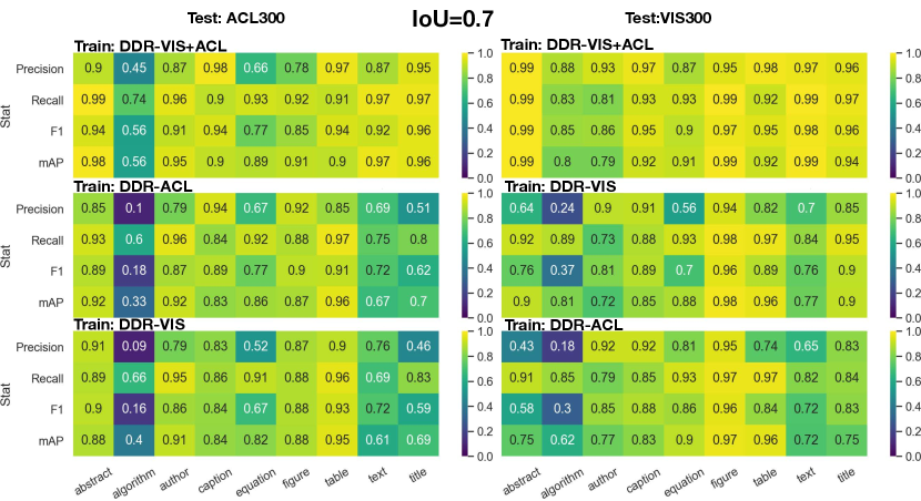
(a)

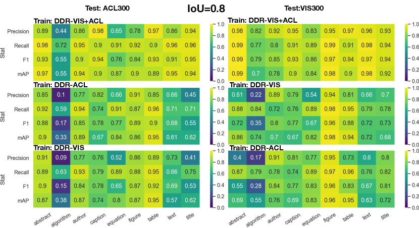
(b)

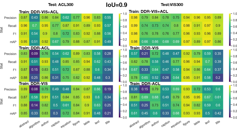
(c)

Figure 14: DDR behavior results from six experiments in Study II.

(a)

Figure 15: Result sample: correctly labelled image with many equations and one figure/caption.

(a)

Figure 16: Result sample: correctly labelled image that has many subimages.

(a)

Figure 17: Result sample: partially incorrectly labeled image: DRR recognized the small figure and its caption but labeled a bullet list as an algorithm and another as an equation. One caption is also missing. This result suggests that we may need to explicitly add ‘bullet list’ class to our training data.

Appendix 0.F Image Rights and Attribution

The VIS30K [9] dataset comprises all the images published at IEEE visualization conferences in each year, rather than just a few samples. All image files are copyrighted and for most the copyright is owned by IEEE. The dataset was released on IEEE Data Port [26]. We thank IEEE for dedicating tools like this to support the Open Science Movement. All ACL papers are from the ACL Anthology website.

References

- [1] Github: Tensorpack Faster R-CNN. Online (Feb 2021), https://github.com/tensorpack/tensorpack/tree/master/examples/FasterRCNN
- [2] Abadi, M., Barham, P., Chen, J., Chen, Z., Davis, A., Dean, J., Devin, M., Ghemawat, S., Irving, G., Isard, M., Kudlur, M., Levenberg, J., Monga, R., Moore, S., Murray, D.G., Steiner, B., Tucker, P., Vasudevan, V., Warden, P., Wicke, M., Yu, Y., Zheng, X., Google Brain: Tensorflow: A system for large-scale machine learning. In: Proc. OSDI. pp. 265–283. USENIX (2016), https://www.usenix.org/conference/osdi16/technical-sessions/presentation/abadi
- [3] Arif, S., Shafait, F.: Table detection in document images using foreground and background features. In: Proc. DICTA. pp. 245–252. IEEE, Piscataway, NJ, USA (2018) doi: 10 . 1109/DICTA . 2018 . 8615795
- [4] Battle, L., Duan, P., Miranda, Z., Mukusheva, D., Chang, R., Stonebraker, M.: Beagle: Automated extraction and interpretation of visualizations from the web. In: Proc. CHI. pp. 594:1–594:8. ACM, New York (2018) doi: 10 . 1145/3173574 . 3174168
- [5] Borkin, M.A., Vo, A.A., Bylinskii, Z., Isola, P., Sunkavalli, S., Oliva, A., Pfister, H.: What makes a visualization memorable? IEEE Trans. Vis. Comput. Graph. 19(12), 2306–2315 (2013) doi: 10 . 1109/TVCG . 2013 . 234
- [6] Caragea, C., Wu, J., Ciobanu, A., Williams, K., Fernández-Ramírez, J., Chen, H.H., Wu, Z., Giles, L.: CiteSeerx: A scholarly big dataset. In: Proc. ECIR. pp. 311–322. Springer, Cham, Switzerland (2014) doi: 10 . 1007/978-3-319-06028-6_26
- [7] Chatzimparmpas, A., Jusufi, I.: The state of the art in enhancing trust in machine learning models with the use of visualizations. Comput. Graph. Forum 39(3), 713–756 (2020) doi: 10 . 1111/cgf . 14034
- [8] Chen, J., Ling, M., Li, R., Isenberg, P., Isenberg, T., Sedlmair, M., Möller, T., Laramee, R., Shen, H.W., Wünsche, K., Wang, Q.: IEEE VIS figures and tables image dataset. IEEE Dataport (2020), https://visimagenavigator.github.io/ doi: 10 . 21227/4hy6-vh52
- [9] Chen, J., Ling, M., Li, R., Isenberg, P., Isenberg, T., Sedlmair, M., Möller, T., Laramee, R.S., Shen, H.W., Wünsche, K., Wang, Q.: VIS30K: A collection of figures and tables from IEEE visualization conference publications. IEEE Trans. Vis. Comput. Graph. 27 (2021), to appear doi: 10 . 1109/TVCG . 2021 . 3054916
- [10] Choudhury, S.R., Mitra, P., Giles, C.L.: Automatic extraction of figures from scholarly documents. In: Proc. DocEng. pp. 47–50. ACM, New York (2015) doi: 10 . 1145/2682571 . 2797085
- [11] Clark, C., Divvala, S.: Looking beyond text: Extracting figures, tables and captions from computer science papers. In: Workshops at the 29th AAAI Conference on Artificial Intelligence (2015), https://aaai.org/ocs/index.php/WS/AAAIW15/paper/view/10092
- [12] Clark, C., Divvala, S.: PDFFigures 2.0: Mining figures from research papers. In: Proc. JCDL. pp. 143–152. ACM, New York (2016) doi: 10 . 1145/2910896 . 2910904
- [13] Davila, K., Setlur, S., Doermann, D., Bhargava, U.K., Govindaraju, V.: Chart mining: A survey of methods for automated chart analysis. IEEE Trans. Pattern Anal. Mach. Intell. 43 (2021), to appear doi: 10 . 1109/TPAMI . 2020 . 2992028
- [14] Dong, X., Gabrilovich, E., Heitz, G., Horn, W., Lao, N., Murphy, K., Strohmann, T., Sun, S., Zhang, W.: Knowledge vault: A web-scale approach to probabilistic knowledge fusion. In: Proc. KDD. pp. 601–610. ACM, New York (2014) doi: 10 . 1145/2623330 . 2623623
- [15] Dosovitskiy, A., Fischer, P., Ilg, E., Häusser, P., Hazırbaş, C., Golkov, V., van der Smagt, P., Cremers, D., Brox, T.: Flownet: Learning optical flow with convolutional networks. In: Proc. ICCV. pp. 2758–2766. IEEE CS, Los Alamitos (2015) doi: 10 . 1109/ICCV . 2015 . 316
- [16] Funke, C.M., Borowski, J., Stosio, K., Brendel, W., Wallis, T.S., Bethge, M.: Five points to check when comparing visual perception in humans and machines. Journal of Vision 21(3), 1–23 (2021) doi: 10 . 1167/jov . 21 . 3 . 16
- [17] Geirhos, R., Rubisch, P., Michaelis, C., Bethge, M., Wichmann, F.A., Brendel, W.: ImageNet-trained CNNs are biased towards texture; increasing shape bias improves accuracy and robustness. No. 1811.12231 (2018), https://arxiv.org/abs/1811.12231
- [18] Giles, C.L., Bollacker, K.D., Lawrence, S.: CiteSeer: An automatic citation indexing system. In: Proc. DL. pp. 89–98. ACM, New York (1998) doi: 10 . 1145/276675 . 276685
- [19] He, D., Cohen, S., Price, B., Kifer, D., Giles, C.L.: Multi-scale multi-task FCN for semantic page segmentation and table detection. In: Proc. ICDAR. pp. 254–261. IEEE CS, Los Alamitos (2017) doi: 10 . 1109/ICDAR . 2017 . 50
- [20] James, S., Johns, E.: 3D simulation for robot arm control with deep Q-learning. No. 1609.03759 (2016), https://arxiv.org/abs/1609.03759
- [21] Katona, G.: Component Extraction from Scientific Publications using Convolutional Neural Networks. Master’s thesis, Computer Science Dept., University of Vienna, Austria (2019)
- [22] Krishna, R., Zhu, Y., Groth, O., Johnson, J., Hata, K., Kravitz, J., Chen, S., Kalantidis, Y., Li, L.J., Shamma, D.A., Bernstein, M.S., Li, F.F.: Visual genome: Connecting language and vision using crowdsourced dense image annotations. Int. J. Comput. Vis. 123(1), 32–73 (2017) doi: 10 . 1007/s11263-016-0981-7
- [23] Li, M., Xu, Y., Cui, L., Huang, S., Wei, F., Li, Z., Zhou, M.: DocBank: A benchmark dataset for document layout analysis. In: Proc. COLING. pp. 949–960. ICCL, Praha, Czech Republic (2020) doi: 10 . 18653/v1/2020 . coling-main . 82
- [24] Li, R., Chen, J.: Toward a deep understanding of what makes a scientific visualization memorable. In: Proc. SciVis. pp. 26–31. IEEE CS, Los Alamitos (2018) doi: 10 . 1109/SciVis . 2018 . 8823764
- [25] Ling, M., Chen, J.: DeepPaperComposer: A simple solution for training data preparation for parsing research papers. In: Proc. EMNLP/Scholarly Document Processing. pp. 91–96. ACL, Stroudsburg, PA, USA (2020) doi: 10 . 18653/v1/2020 . sdp-1 . 10
- [26] Ling, M., Chen, J., Möller, T., Isenberg, P., Isenberg, T., Sedlmair, M., Laramee, R., Shen, H.W., Wu, J., Giles, C.L.: Three benchmark datasets for scholarly article layout analysis. IEEE Dataport (2020) doi: 10 . 21227/326q-bf39
- [27] Lo, K., Wang, L.L., Neumann, M., Kinney, R., Weld, D.S.: S2ORC: The semantic scholar open research corpus. In: Proc. ACL. pp. 4969–4983. ACL, Stroudsburg, PA, USA (2020) doi: 10 . 18653/v1/2020 . acl-main . 447
- [28] Lopez, P.: GROBID: Combining automatic bibliographic data recognition and term extraction for scholarship publications. In: Proc. ECDL. pp. 473–474. Springer, Berlin (2009) doi: 10 . 1007/978-3-642-04346-8_62
- [29] Mayer, N., Ilg, E., Häusser, P., Fischer, P., Cremers, D., Dosovitskiy, A., Brox, T.: A large dataset to train convolutional networks for disparity, optical flow, and scene flow estimation. In: Proc. CVPR. pp. 4040–4048. IEEE CS, Los Alamitos (2016) doi: 10 . 1109/CVPR . 2016 . 438
- [30] Poppler: Poppler. Dataset and online search (2014), https://poppler.freedesktop.org/
- [31] Praczyk, P., Nogueras-Iso, J.: A semantic approach for the annotation of figures: Application to high-energy physics. In: Proc. MTSR. pp. 302–314. Springer, Berlin (2013) doi: 10 . 1007/978-3-319-03437-9_30
- [32] Ren, S., He, K., Girshick, R., Sun, J.: Faster R-CNN: Towards real-time object detection with region proposal networks. IEEE Trans. Pattern Anal. Mach. Intell. 39(6), 1137–1149 (2017) doi: 10 . 1109/TPAMI . 2016 . 2577031
- [33] Rolnick, D., Veit, A., Belongie, S., Shavit, N.: Deep learning is robust to massive label noise. arXiv preprint arXiv:1705.10694 (2017), https://arxiv.org/abs/1705.10694
- [34] Sadeghi, F., Levine, S.: CAD2RL: Real single-image flight without a single real image. In: Proc. RSS. pp. 34:1–34:10. RSS Foundation (2017) doi: 10 . 15607/RSS . 2017 . XIII . 034
- [35] Siegel, N., Horvitz, Z., Levin, R., Divvala, S., Farhadi, A.: FigureSeer: Parsing result-figures in research papers. In: Proc. ECCV. pp. 664–680. Springer, Berlin (2016) doi: 10 . 1007/978-3-319-46478-7_41
- [36] Siegel, N., Lourie, N., Power, R., Ammar, W.: Extracting scientific figures with distantly supervised neural networks. In: Proc. JCDL. pp. 223–232. ACM, New York (2018) doi: 10 . 1145/3197026 . 3197040
- [37] Sinha, A., Shen, Z., Song, Y., Ma, H., Eide, D., Hsu, B.J., Wang, K.: An overview of Microsoft Academic Service (MAS) and applications. In: Proc. WWW. pp. 243–246. ACM, New York (2015) doi: 10 . 1145/2740908 . 2742839
- [38] Song, S., Lichtenberg, S.P., Xiao, J.: SUN RGB-D: A RGB-D scene understanding benchmark suite. In: Proc. CVPR. pp. 567–576. IEEE CS, Los Alamitos (2015) doi: 10 . 1109/CVPR . 2015 . 7298655
- [39] Stribling, J., Krohn, M., Aguayo, D.: SCIgen – An automatic CS paper generator. Online tool: https://pdos.csail.mit.edu/archive/scigen/ (2005)
- [40] Tobin, J., Fong, R., Ray, A., Schneider, J., Zaremba, W., Abbeel, P.: Domain randomization for transferring deep neural networks from simulation to the real world. In: Proc. IROS. pp. 23–30. IEEE, Piscataway, NJ, USA (2017) doi: 10 . 1109/IROS . 2017 . 8202133
- [41] Tremblay, J., Prakash, A., Acuna, D., Brophy, M., Jampani, V., Anil, C., To, T., Cameracci, E., Boochoon, S., Birchfield, S.: Training deep networks with synthetic data: Bridging the reality gap by domain randomization. In: Proc. CVPRW. pp. 969–977. IEEE CS, Los Alamitos (2018) doi: 10 . 1109/CVPRW . 2018 . 00143
- [42] Yang, X., Yumer, E., Asente, P., Kraley, M., Kifer, D., Lee Giles, C.: Learning to extract semantic structure from documents using multimodal fully convolutional neural networks. In: Proc. CVPR. pp. 5315–5324. IEEE CS, Los Alamitos (2017) doi: 10 . 1109/CVPR . 2017 . 462
- [43] Zhong, X., Tang, J., Yepes, A.J.: PubLayNet: Largest dataset ever for document layout analysis. In: Proc. ICDAR. pp. 1015–1022. IEEE CS, Los Alamitos (2019) doi: 10 . 1109/ICDAR . 2019 . 00166