Abstract

Reparameterization (RP) and likelihood ratio (LR) gradient estimators are used to estimate gradients of expectations throughout machine learning and reinforcement learning; however, they are usually explained as simple mathematical tricks, with no insight into their nature. We use a first principles approach to explain that LR and RP are alternative methods of keeping track of the movement of probability mass, and the two are connected via the divergence theorem. Moreover, we show that the space of all possible estimators combining LR and RP can be completely parameterized by a flow field ${\bm{u}}({\bm{x}})$ and an importance sampling distribution $q({\bm{x}})$. We prove that there cannot exist a single-sample estimator of this type outside our characterized space, thus, clarifying where we should be searching for better Monte Carlo gradient estimators.

1 INTRODUCTION

Both likelihood ratio (LR) gradients (Glynn,, 1990; Williams,, 1992) and reparameterization (RP) gradients (Rezende et al.,, 2014; Kingma and Welling,, 2013) give unbiased estimates of the gradient of an expectation w.r.t. the parameters of the distribution: $\frac{\textup{d}\hfill}{\textup{d}\theta\hfill}\mathbb{E}_{p\left(x;\theta\right)}\left[\phi(x)\right]$. This gradient estimation problem is fundamental in machine learning (Mohamed et al.,, 2019), where the gradients are used for optimization. LR is the basis of many reinforcement learning (RL) (Sutton and Barto,, 1998; Schulman et al., 2015b, ; Schulman et al.,, 2017; Sutton et al.,, 2000; Peters and Schaal,, 2008) and evolutionary algorithms (Wierstra et al.,, 2008; Salimans et al.,, 2017; Ha and Schmidhuber,, 2018; Conti et al.,, 2018). In RL, $\phi(x)$ represents the sum of rewards, and $\theta$ are the policy parameters. RP, on the other hand, is the backbone of stochastic variational inference (Hoffman et al.,, 2013), where $\phi(x)$ is the evidence lower bound, and $\theta$ are the variational parameters. For example, RP is used in autoencoders (Kingma and Welling,, 2013). There is a vast body of research on both estimators (App. A), and there is no clear winner among RP and LR—both have advantages and disadvantages.

LR uses samples of the value of the function $\phi(x)$ to estimate the gradient, and is usually derived as

$$\frac{\textup{d}\hfill}{\textup{d}\theta\hfill}\mathbb{E}_{p\left(x;\theta\right)}\left[\phi(x)\right] =\int\frac{\textup{d}p\left(x;\theta\right)\hfill}{\textup{d}\theta\hfill}\phi(x)\textup{d}x$$ (1)

$$=\int p\left(x;\theta\right)\frac{1}{p\left(x;\theta\right)}\frac{\textup{d}p\left(x;\theta\right)\hfill}{\textup{d}\theta\hfill}\phi(x)\textup{d}x$$

$$=\int p\left(x;\theta\right)\frac{\textup{d}\log p\left(x;\theta\right)\hfill}{\textup{d}\theta\hfill}\phi(x)\textup{d}x$$

$$=\mathbb{E}_{p\left(x;\theta\right)}\left[\frac{\textup{d}\log p\left(x;\theta\right)\hfill}{\textup{d}\theta\hfill}\phi(x)\right].$$

On the other hand, RP uses samples of the gradient of the function $\frac{\textup{d}\phi(x)\hfill}{\textup{d}x\hfill}$, and it is derived by defining a mapping $g(\epsilon;\theta)=x$, where $\epsilon$ is sampled from a fixed simple distribution, $p(\epsilon)$, independent of $\theta$, but $x$ ends up being sampled from the desired distribution. For example, if $x$ is Gaussian, $x~{}\sim~{}\mathcal{N}(\mu,\sigma)$, then the required mapping is $g(\epsilon;\theta)=\mu+\sigma\epsilon$, where $\epsilon~{}\sim~{}\mathcal{N}(0,1)$, and the RP gradient is derived as

$$\frac{\textup{d}\hfill}{\textup{d}\theta\hfill}\mathbb{E}_{p\left(x;\theta\right)}\left[\phi(x)\right] =\frac{\textup{d}\hfill}{\textup{d}\theta\hfill}\mathbb{E}_{\epsilon\sim\mathcal{N}(0,1)}\left[\phi\left(g(\epsilon;\theta)\right)\right]$$ (2)

$$=\mathbb{E}_{\epsilon\sim\mathcal{N}(0,1)}\left[\frac{\textup{d}\phi\left(g(\epsilon;\theta)\right)\hfill}{\textup{d}\theta\hfill}\right]$$

$$=\mathbb{E}_{\epsilon\sim\mathcal{N}(0,1)}\left[\frac{\textup{d}\phi\left(g(\epsilon;\theta)\right)\hfill}{\textup{d}g\hfill}\frac{\textup{d}g(\epsilon;\theta)\hfill}{\textup{d}\theta\hfill}\right],$$

where $\theta=[\mu,\sigma]$, $\frac{\textup{d}g\hfill}{\textup{d}\mu\hfill}=1$, $\frac{\textup{d}g\hfill}{\textup{d}\sigma\hfill}=\epsilon$ and $\frac{\textup{d}\phi\left(g(\epsilon;\theta)\right)\hfill}{\textup{d}g\hfill}=\frac{\textup{d}\phi\left(x\right)\hfill}{\textup{d}x\hfill}$.

What do these derivations mean, and what is the relationship between the two methods? We give two possible answers to this question: (i) we give a first principles explanation that these are different methods of keeping track of the movement of probability mass (Sec. 3), (ii) we show that RP and LR are duals under the divergence theorem when considering the integral of a probability mass flow (Sec. 4). Our theory gives a physical insight by analogy to fluid dynamics, and allows for intuitive visualizations. Our main technical result is in Thm. 3, where we formalize a generalized estimator that includes all previous LR and RP gradients as special cases, and we prove that there cannot exist an estimator of this type outside our characterized space. Finally, we advocate for a systematic approach in the search for novel gradient estimators (Sec. 5).

2 PRELIMINARIES

We introduce some preliminaries. In Eq. (4) we introduce a general form of all gradient estimators of the LR–RP type. Sec. 2.2 explains that the introduced equation indeed includes RP as a special case. Sec. 2.3 introduces the Monte Carlo (MC) integration principle, which provides a link between integral expressions and the corresponding gradient estimators. Sec. 2.4 introduces previous works on the relationship between LR and RP, and the limitations of these works. Sec. 2.5 gives basic knowledge about fluid dynamics and the divergence theorem necessary for understanding Sec. 4.

2.1 Setup

Problem statement.

Given one sample ${\bm{x}}\sim q({\bm{x}})$, and while being allowed to evaluate $\phi({\bm{x}})$ and $\nabla_{{\bm{x}}}\phi({\bm{x}})$, construct an estimator, $E_{\theta_{i}}$, which may depend on ${\bm{x}},\phi({\bm{x}})$ and $\nabla_{{\bm{x}}}\phi({\bm{x}})$, s.t.

$$\mathbb{E}_{q({\bm{x}})}\left[E_{\theta_{i}}\right]=\frac{\textup{d}\hfill}{\textup{d}\theta_{i}\hfill}\mathbb{E}_{p({\bm{x}})}\left[\phi({\bm{x}})\right].$$ (3)

To obtain an estimator for the full gradient w.r.t. $\theta$ (as opposed to the derivative w.r.t. one element of the parameters $\theta_{i}$), we can stack the estimators together: $E_{\theta}=[E_{\theta_{1}},E_{\theta_{2}},\ldots]$. Note that, while in the problem statement we consider one sample, ${\bm{x}}\sim q({\bm{x}})$, the estimators can also be used with multiple samples in a batch by averaging the estimates together. The main reason we explicitly write out this problem statement is to emphasize the format based on having access to $\phi({\bm{x}})$ and $\nabla_{{\bm{x}}}\phi({\bm{x}})$. We will further restrict our discussion to estimators having the following product form:

$$E_{\theta_{i}}={\bm{u}}_{\theta_{i}}({\bm{x}})\cdot\nabla_{{\bm{x}}}\phi({\bm{x}})+\psi_{\theta_{i}}({\bm{x}})\phi({\bm{x}}),$$ (4)

where ${\bm{u}}_{\theta_{i}}({\bm{x}})$ is an arbitrary vector field, and $\psi_{\theta_{i}}({\bm{x}})$ is an arbitrary scalar field (a function). Essentially, this equation is taking a weighted sum of the partial derivatives and value of $\phi({\bm{x}})$, with a different weighting defined at each ${\bm{x}}$. Both LR and RP belong to this class of gradient estimators. Assuming that the sampling distribution is $q({\bm{x}})=p({\bm{x}};\theta)$, we obtain LR by setting ${\bm{u}}_{\theta_{i}}({\bm{x}})={\bm{0}}$, and $\psi_{\theta_{i}}({\bm{x}})=\frac{\textup{d}\log p\left({\bm{x}};\theta\right)\hfill}{\textup{d}\theta_{i}\hfill}$. Note, that in Eq. (2), RP also has a $\frac{\textup{d}\phi(x)\hfill}{\textup{d}x\hfill}$ term, so it seems that it may also be described by the class of estimators in Eq. (4); however, there is a coordinate transformation to the $\epsilon$-space, which may cause some confusion. In Sec. 2.2, we clear this confusion and show that, indeed, RP also belongs to the given class of estimators.

2.2 Coordinate Transformations

In Eq. (2), $\frac{\textup{d}\phi\left(g(\epsilon;\theta)\right)\hfill}{\textup{d}g\hfill}=\frac{\textup{d}\phi\left(x\right)\hfill}{\textup{d}x\hfill}$ requires no reference to $\epsilon$, and could be computed by just knowing the $x$ corresponding to the $\epsilon$. Moreover, each $\epsilon$ is always in a one-to-one correspondence with a particular $x$. Therefore, the whole estimator $\frac{\textup{d}\phi\left(g(\epsilon;\theta)\right)\hfill}{\textup{d}g\hfill}\frac{\textup{d}g(\epsilon;\theta)\hfill}{\textup{d}\theta\hfill}$ could be computed by directly sampling $x\sim p(x;\theta)$, converting it to the corresponding $\epsilon$, and computing the estimator. We denote the mapping from $x$ to $\epsilon$ with $\epsilon=S(x;\theta)$, and call $S$ the standardization function. This function is the inverse of the RP transformation, $x=g(\epsilon;\theta)$, defined in the introduction. The standardization function was used in implicit reparameterization gradients (Figurnov et al.,, 2018) to create an estimator without reference to $\epsilon$ that is applicable to a broader class of distributions than typical reparameterizations. The main point we wanted to emphasize here is that there is no need to refer to coordinate transformations at all to define RP gradients, and the $\epsilon$-space is just a convenience that makes it easier to apply RP using automatic differentiation. In particular, given a sample $x\sim p(x;\theta)$, the RP estimator can be written as $\frac{\textup{d}\phi(x)\hfill}{\textup{d}x\hfill}\left.\frac{\partial g(\epsilon;\theta)\hfill}{\partial\theta\hfill}\right|_{\epsilon=S(x;\theta)}$, where $\left.\frac{\partial g(\epsilon;\theta)\hfill}{\partial\theta_{i}\hfill}\right|_{\epsilon=S(x;\theta)}$ corresponds to ${\bm{u}}_{\theta_{i}}({\bm{x}})$.

2.3 Importance Sampling/MC Integration

Definition 1 (Integral expression).

An integral expression is denoted by $\int_{\Omega}f(x)\textup{d}x$, and it comprises the domain of integration $\Omega$, the function $f(x)$, and the measure of integration corresponding to $\textup{d}x$.

The reason we make such a seemingly trivial definition is to distinguish between the integral expression and the value of the integral. For example, the integral expressions corresponding to the LR gradient (Eq. (1)) and the RP gradient (Eq. (2)) are different, but they evaluate to the same quantity. Thus, there is a duality between the integrals; however, it is not clear how this duality arises. In Sec. 4 we explain that the integrals are duals under the divergence theorem. Next, we explain how these integral expressions are related to the gradient estimators via importance sampling.

MC integration:

Any integral $\int f(x)~{}\textup{d}x$ can be estimated using Monte Carlo integration as follows:

$$\int f(x)~{}\textup{d}x =\int q(x)\frac{f(x)}{q(x)}\textup{d}x$$ (5)

$$=\mathbb{E}_{q(x)}\left[\frac{f(x)}{q(x)}\right],$$

where we are importance sampling from $x\sim q(x)$. From this method, we see that the LR gradient estimator $E_{\mathrm{LR}}=\left.\frac{\textup{d}p(x;\theta)\hfill}{\textup{d}\theta\hfill}\phi(x)\middle/q(x)\right.$ arises by applying the MC integration principle to the integral expression $I_{\mathrm{LR}}=\int\frac{\textup{d}p(x;\theta)\hfill}{\textup{d}\theta\hfill}\phi(x)\textup{d}x$, when $q(x)=p(x;\theta)$. Moreover, the integral expression corresponding to RP is given by $I_{\mathrm{RP}}=\int p(x;\theta)\frac{\textup{d}\phi(x)\hfill}{\textup{d}x\hfill}\left.\frac{\partial g(\epsilon;\theta)\hfill}{\partial\theta\hfill}\right|_{\epsilon=S(x;\theta)}\textup{d}x$, and the gradient estimator for general $q(x)$ is $E_{\mathrm{RP}}~{}=~{}\frac{p(x;\theta)}{q(x)}\frac{\textup{d}\phi(x)\hfill}{\textup{d}x\hfill}\left.\frac{\partial g(\epsilon;\theta)\hfill}{\partial\theta\hfill}\right|_{\epsilon=S(x;\theta)}$. In general, given an integral expression for a gradient estimator, one can always construct the estimator by directly applying MC integration. But the reverse is also true—given an estimator, $E$, one can always construct the integral expression as $I=\int E\textup{d}q$, where the $\textup{d}q$ indicates that we are integrating w.r.t. the measure corresponding to $q$ ($\textup{d}q$ can be considered as being equivalent to $q(x)\textup{d}x$). Thus, there is a one-to-one correspondence between the estimator and the integral expression, given the sampling distribution, $q(x)$. Previously, in machine learning (ML), importance sampling was suggested as a principle for LR (Jie and Abbeel,, 2010), but the link to RP has not been discussed in ML. We on the other hand, suggest importance sampling as a key component of any gradient estimator, including RP.

2.4 Prior Work on the Relationship between LR and RP Gradient Estimators

Measure theoretic view:

LR and RP gradients are well-studied in operations research (L’Ecuyer,, 1991), where their relationship has been described in terms of measure theory (L’Ecuyer,, 1990). They defined the problem as finding the gradient of an expectation of a function $\phi(\omega;\theta)$ where the expectation is taken w.r.t. a probability measure $P_{\theta}$. Here, $\omega$ represents a sample in this space, and, unlike our previous definition, $\phi$ may also depend on $\theta$. Then, by sampling w.r.t. a different probability measure $G$, independent of $\theta$, on the same space, the expectation can be written as

$$\int\phi(\omega;\theta)\textup{d}P_{\theta}=\int\phi(\omega;\theta)\frac{\textup{d}P_{\theta}\hfill}{\textup{d}G\hfill}\textup{d}G=\int\phi(\omega;\theta)L_{\theta}\textup{d}G,$$ (6)

where $L_{\theta}=\frac{\textup{d}P_{\theta}\hfill}{\textup{d}G\hfill}$ is the Radon-Nikodym derivative, a function $f$, s.t. $P_{\theta}(A)=\int_{A}f\textup{d}G$, where $P_{\theta}(A)$ denotes the measure of set $A$. If $p(\omega;\theta)$ and $q(\omega)$ are the pdf’s of $P_{\theta}$ and $G$ respectively, then we simply have $L_{\theta}=\frac{p\left(\omega;\theta\right)}{q(\omega)}$ is the likelihood ratio. Differentiating w.r.t. $\theta$ gives

$$\frac{\textup{d}\hfill}{\textup{d}\theta\hfill}\int\phi(\omega;\theta)L_{\theta}\textup{d}G=\int\frac{\textup{d}\phi(\omega;\theta)\hfill}{\textup{d}\theta\hfill}L_{\theta}+\phi(\omega;\theta)\frac{\textup{d}L_{\theta}\hfill}{\textup{d}\theta\hfill}\textup{d}G.$$ (7)

Now, depending on how the probability space $P_{\theta}$ is defined, one obtains either the likelihood ratio gradient or the reparameterization gradient. If $\omega\coloneqq x$, then $\phi$ is independent of $\theta$, so $\frac{\textup{d}\phi(\omega;\theta)\hfill}{\textup{d}\theta\hfill}=0$, and one obtains the likelihood ratio gradient term $\frac{\textup{d}L_{\theta}\hfill}{\textup{d}\theta\hfill}=\frac{\textup{d}p\left(x;\theta\right)\hfill}{\textup{d}\theta\hfill}/q(x)$, which is the same as in Eq. (1), except that importance sampling from $q$ is used (set $q=p$ to get exactly the LR gradient). On the other hand, if $\omega\coloneqq\epsilon$, and $\phi(\epsilon;\theta)$ is defined as $\phi\left(g(\epsilon;\theta)\right)$, then $L$ is independent of $\theta$, and one is left with only the reparameterization gradient term $\frac{\textup{d}\phi(\epsilon;\theta)\hfill}{\textup{d}\theta\hfill}$, as in Eq. (2).

A strength of this view is that it shows that LR and RP lie at opposite ends of a spectrum of estimators using both derivative and value information of $\phi$. However, the additional intuition is still limited, as the theory does not explain how these opposite ends are related, and how to convert between the two—the theory only says that if one can choose probability spaces with specific properties, one obtains either RP or LR, but it does not explain how to achieve the desired properties.

Stein’s identity/integration by parts:

Another work on policy gradients (Liu et al.,, 2017) showed a connection between RP and LR via Stein’s identity:

$$\int p\left(x;\theta\right)\left(\frac{\textup{d}\log p\left(x;\theta\right)\hfill}{\textup{d}x\hfill}\phi(x)+\frac{\textup{d}\phi(x)\hfill}{\textup{d}x\hfill}\right)\textup{d}x=0;$$ (8)

however, note that the derivative here is w.r.t. $x$, not $\theta$. They showed algebraically that it generalizes to derivatives w.r.t. $\theta$, but to do so, they put infinitesimal Gaussian noise on $x$, and the additional intuition from their work is still limited.

Ranganath et al., (2016) presented a derivation based on integration by parts, which can be seen as a generalized view compared to Stein’s identity. We present this derivation and discuss it below.

Integration by parts is described by the identity:

$$\int_{a}^{b}f(x)h(x)\textup{d}x$$ (9)

$$=\left[\int_{a}^{x}f(z)\textup{d}z~{}h(x)\right]_{a}^{b}-\int_{a}^{b}\int_{a}^{x}f(z)\textup{d}z~{}\frac{\textup{d}h(x)\hfill}{\textup{d}x\hfill}\textup{d}x.$$

We apply this identity on the integral for LR:

$$\int_{-\infty}^{+\infty}\frac{\textup{d}p(x;\theta)\hfill}{\textup{d}\theta\hfill}\phi(x)\textup{d}x=\left[\int_{-\infty}^{x}\frac{\textup{d}p(z;\theta)\hfill}{\textup{d}\theta\hfill}\textup{d}z~{}\phi(x)\right]_{-\infty}^{+\infty}$$ (10)

$$-\int_{-\infty}^{+\infty}\int_{-\infty}^{x}\frac{\textup{d}p(z;\theta)\hfill}{\textup{d}\theta\hfill}\textup{d}z~{}\frac{\textup{d}\phi(x)\hfill}{\textup{d}x\hfill}\textup{d}x.$$

We can simplify as follows:

$$\int_{-\infty}^{x}\frac{\textup{d}p(z;\theta)\hfill}{\textup{d}\theta\hfill}\textup{d}z=\frac{\textup{d}\hfill}{\textup{d}\theta\hfill}\int_{-\infty}^{x}p(z;\theta)\textup{d}z=\frac{\textup{d}Q(x;\theta)\hfill}{\textup{d}\theta\hfill},$$ (11)

where $Q(x;\theta)$ is the cumulative density function. The first term in Eq. (10) disappears because $\frac{\textup{d}Q(x;\theta)\hfill}{\textup{d}\theta\hfill}=0$ at $x=\pm\infty$, and we end up with

$$\int p(x;\theta)\left(\frac{-1}{p(x;\theta)}\frac{\textup{d}Q(x;\theta)\hfill}{\textup{d}\theta\hfill}\right)\frac{\textup{d}\phi(x)\hfill}{\textup{d}x\hfill}\textup{d}x.$$ (12)

We can see that $\frac{-1}{p(x;\theta)}\frac{\textup{d}Q(x;\theta)\hfill}{\textup{d}\theta\hfill}$ is equivalent to ${\bm{u}}_{\theta_{i}}({\bm{x}})$ in Eq. (4). In the one-dimensional case, it turns out that this estimation method is the same as RP; however, the theory is still limited in several ways: (i) the derivation only considers one particular ${\bm{u}}_{\theta_{i}}({\bm{x}})$ as opposed to an arbitrary one, (ii) in multiple dimensions, there are other RP gradients not conforming to this equation (Jankowiak and Obermeyer,, 2018), (iii) the additional intuition from the derivation is limited—it appears to be just another “trick”. It was suggested that the derivation is insightful, because the analytic computation of the zero term, $\left[\int_{-\infty}^{x}\frac{\textup{d}p(z;\theta)\hfill}{\textup{d}\theta\hfill}\textup{d}z~{}\phi(x)\right]_{-\infty}^{+\infty}=0$, is a reason for why RP has lower variance than LR (Ranganath et al.,, 2016; Cong et al.,, 2019). However, this argument is unsound because, on the contrary, adding a negatively correlated 0-mean random variable to the estimator, known as a control variate, is a common technique to reduce the variance (Greensmith et al., 2004a, ). Moreover, RP is not guaranteed to have lower variance than LR. For example, Parmas et al., (2018) showed a practical situation where LR is $10^{6}$ more accurate than RP due to chaotic dynamics in the system. Other works showed toy problems where LR outperforms RP (Gal,, 2016; Mohamed et al.,, 2019). Finally, it is unclear why analytically integrating a variable added to the integral expression should be related to the variance to begin with (as opposed to integrating a random variable in the estimator, a technique known as conditioning/Rao-Blackwellization (Owen,, 2013)).

In conclusion, previous theories of the connection between RP and LR are still limited.

2.5 Vector Calculus and Fluid Dynamics

Our unified theory in Sec. 4 relies on considering a “flow” of probability mass, so we give some background information. We illustrate the background in the 3-dimensional case, but it generalizes straightforwardly to higher dimensions.

Notation:

${\bm{F}}=[F_{x}(x,y,z),F_{y}(x,y,z),F_{z}(x,y,z)]$ is a vector field.
$\phi(x,y,z)$ is a scalar field (a scalar function).
Divergence operator: $\nabla\cdot{\bm{F}}=\frac{\partial F_{x}\hfill}{\partial x\hfill}+\frac{\partial F_{y}\hfill}{\partial y\hfill}+\frac{\partial F_{z}\hfill}{\partial z\hfill}$.
Gradient operator: $\nabla\phi=\left[\frac{\partial\phi\hfill}{\partial x\hfill},\frac{\partial\phi\hfill}{\partial y\hfill},\frac{\partial\phi\hfill}{\partial z\hfill}\right]$.

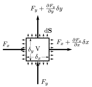
Figure 1: Illustration of the divergence theorem.

The vector field ${\bm{F}}$ could be, for example, thought of as a local flow velocity of some fluid. If ${\bm{F}}$ is the density flow rate, then the divergence operator essentially measures how much the density is decreasing at a point. If the outflow is larger than the inflow, then the density decreases and vice versa. The divergence theorem, illustrated in Fig. 1, shows how this change in density can be measured in two equivalent ways: one could integrate the divergence across the volume, or one could integrate the inflow and outflow across the surface.

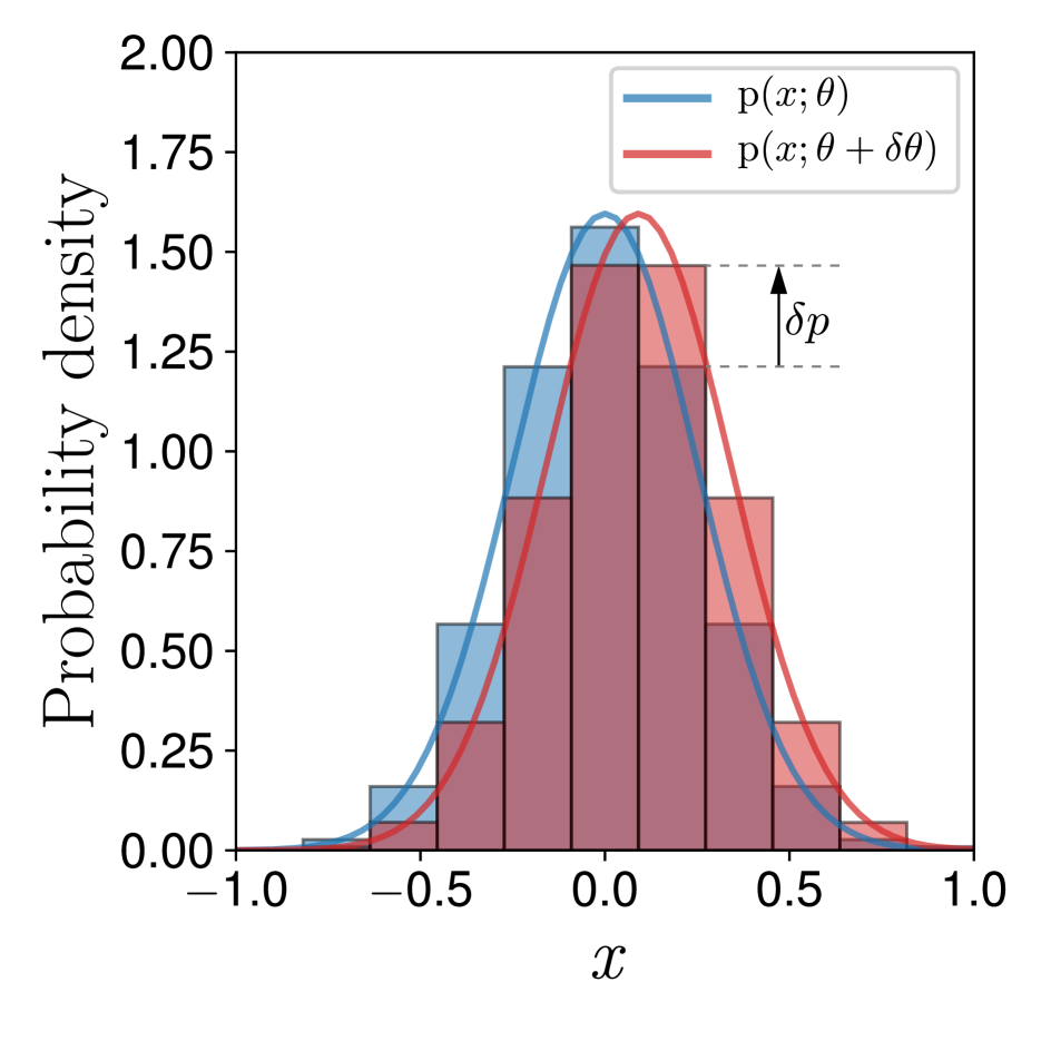
(a) LR probability “boxes”

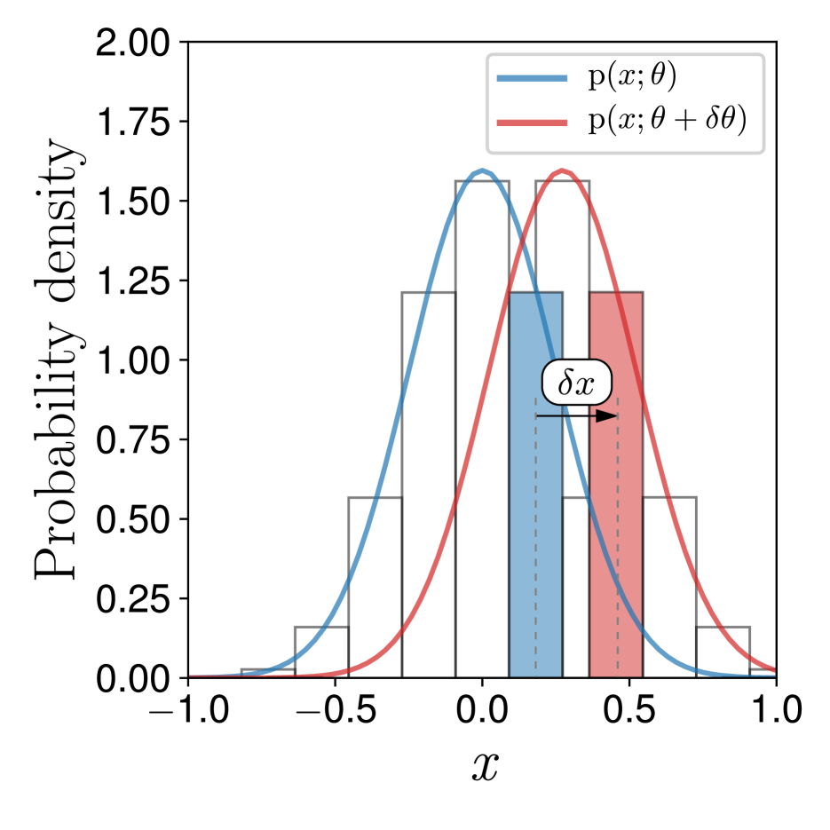
(b) RP probability “boxes”

Figure 2: LR keeps the boundaries of the “boxes” fixed, while RP keeps the probability mass fixed.

Theorem 1 (Divergence theorem).

$$\int_{V}\nabla\cdot{\bm{F}}\textup{d}V=\int_{S}{\bm{F}}\cdot\textup{d}{\bm{S}}.$$ (13)

Proof.

To prove the claim, consider the infinitesimal box in Fig. 1. The divergence can be calculated as

$$\int_{V}\nabla\cdot{\bm{F}}\textup{d}V=\delta x\delta y\left(\frac{\partial F_{x}\hfill}{\partial x\hfill}+\frac{\partial F_{y}\hfill}{\partial y\hfill}\right).$$ (14)

On the other hand, to take the integral across the surface, note that the surface normals point outwards, and the integral becomes

$$\int_{S}{\bm{F}}\cdot\textup{d}{\bm{S}} =\delta_{y}\left(-F_{x}+F_{x}-\frac{\partial F_{x}\hfill}{\partial x\hfill}\delta x\right)$$ (15)

$$~{}~{}~{}+\delta x\left(-F_{y}+F_{y}+\frac{\partial F_{y}\hfill}{\partial y\hfill}\delta y\right)$$

$$=\delta x\delta y\left(\frac{\partial F_{x}\hfill}{\partial x\hfill}+\frac{\partial F_{y}\hfill}{\partial y\hfill}\right),$$

which is the same as the divergence. To generalize this to arbitrarily large volumes, notice that if one stacks the boxes next to each other, then the surface integral across the area where the boxes meet cancels out, and only the integral across the outer surface remains. ∎

For an incompressible flow, the density at any point does not change, and the divergence must be zero.

3 A PROBABILITY “BOXES” VIEW OF LR AND RP GRADIENTS

Here we give our first explanation of the link between LR and RP gradients, illustrated in Fig. 2. In short, LR gradients estimate the change in expectation by measuring how the probability mass assigned to each $\phi(x)$ located at a fixed $x$ changes, whereas RP gradients define “boxes” of fixed probability mass, keep track of where this “box” moves as the parameters $\theta$ change, and measure how the value $\phi$ corresponding to this “box” changes. For the ease of the explanation, consider a discrete space, where $x\sim P(x;\theta)$ can take $N$ possible values. The continuous case can be recovered by letting $N\to\infty$. Fundamentally, the expectation, $\mathbb{E}_{P(x;\theta)}\left[\phi(x)\right]$, is a weighted average of function values $\sum_{i=1}^{N}P(x_{i})\phi(x_{i})$, where the weights sum to one: $\sum_{i=1}^{N}P(x_{i})=1$. Therefore, to determine the expectation, we must determine how the probability mass is allocated to the different $\phi(x_{i})$ values. We can envision two different allocation procedures: (i) for each $\phi(x_{i})$ at a fixed $x_{i}$, we determine how much probability mass $P_{i}$ we assign to it; (ii) we predetermine the sizes of the “boxes” of fixed probability mass $P_{j}$, then, for each box with weight $P_{j}$ we assign one of the available $\phi(x_{i})$ values. Now, to measure the gradient of the expectation, $\frac{\textup{d}\hfill}{\textup{d}\theta\hfill}\mathbb{E}_{P(x;\theta)}\left[\phi(x)\right]$, one must measure how the probability mass is reallocated as the parameters $\theta$ are perturbed. We will see that allocation procedure (i) corresponds to LR gradients, whereas (ii) corresponds to RP gradients. A full formal derivation is given in App. C, but reading it should not be necessary to understand the concept, which we explain intuitively below. To perform the estimation, first note that the gradient is given by $\frac{\textup{d}\hfill}{\textup{d}\theta\hfill}\sum_{i=1}^{N}P(x_{i})\phi(x_{i})=\sum_{i=1}^{N}\frac{\textup{d}\hfill}{\textup{d}\theta\hfill}\bigl{(}P(x_{i})\phi(x_{i})\bigr{)}$.

LR estimator:

In case (i): $\phi(x_{i})$ is fixed, so $\frac{\textup{d}\hfill}{\textup{d}\theta\hfill}\bigl{(}P(x_{i})\phi(x_{i})\bigr{)}=\frac{\textup{d}P(x_{i})\hfill}{\textup{d}\theta\hfill}\phi(x_{i})$, and to estimate the gradient, one must measure how the weight assigned to each particular $\phi(x_{i})$ changes. This corresponds precisely to what the LR gradient estimator does. To see this, first consider that any integral can be estimated by importance sampling from a distribution $q(x)$, and using MC integration, as shown in Eq. (5). Now, we set $q(x)=P(x;\theta)$, sample $x_{i}\sim P(x;\theta)$, and use the gradient estimator $E=\frac{1}{P(x_{i};\theta)}\frac{\textup{d}P(x_{i})\hfill}{\textup{d}\theta\hfill}\phi(x_{i})$. Then this will satisfy $\mathbb{E}_{x_{i}\sim P(x;\theta)}\left[E\right]=\sum_{i=1}^{N}\frac{\textup{d}\hfill}{\textup{d}\theta\hfill}\bigl{(}P(x_{i})\phi(x_{i})\bigr{)}$. Note that $\frac{1}{P(x_{i};\theta)}\frac{\textup{d}P(x_{i};\theta)\hfill}{\textup{d}\theta\hfill}=\frac{\textup{d}\hfill}{\textup{d}\theta\hfill}\log P(x_{i};\theta),$ and we see that it is the same as the LR gradient in Eq. (1). The transformation to the log term is known as the log-derivative trick, and it may appear to be the essence behind the LR gradient. However, actually the multiplication and division by $P(x;\theta)$ is just a special case of the more general MC integration principle. Rather than thinking of the LR gradient in terms of the log-derivative term, it may be better to think of it as simply estimating the integral of the probability gradient by applying the appropriate importance weights. Sometimes, the LR gradient is described as being “kind of like a finite difference gradient” (Salimans et al.,, 2017; Mania et al.,, 2018), but here we see that it is a different concept that does not rely on fitting a straight line between differences of $\phi$ (App. B), but estimates how probability mass is reallocated among different $\phi$ values.

RP estimator:

In case (ii): $P(x_{i})$ is fixed, but $\phi(x_{i})$ may change—such a situation can occur when one has a fixed amount of probability mass $P_{i}$ in the “box”, but the location, $x_{i}$, changes. In this case, we have $\frac{\textup{d}\hfill}{\textup{d}\theta\hfill}\bigl{(}P(x_{i})\phi(x_{i})\bigr{)}=P(x_{i})\frac{\textup{d}\phi(x_{i})\hfill}{\textup{d}\theta\hfill}=P(x_{i})\frac{\textup{d}\phi(x_{i})\hfill}{\textup{d}x_{i}\hfill}\frac{\textup{d}x_{i}\hfill}{\textup{d}\theta\hfill}$, and to estimate the gradient, one must measure how the function value $\phi$ in the “box” changes. For example, consider shifting the mean location of a Gaussian distribution by $\delta\mu$, hence, also shifting the location of each of the “boxes” by the same quantity, as depicted in Fig. 2. The probability inside the box would stay fixed, but the function value $\phi$ would change. This situation corresponds to the RP gradient in Eq. (2). In this case, the position of the “box” is defined by $x_{i}:=g(\epsilon_{i};\theta)$, and the probability density assigned to $\epsilon_{i}$ stays fixed at $p(\epsilon_{i})$. Finally, note that we can construct an estimator $E=\frac{\textup{d}\phi(x_{i})\hfill}{\textup{d}x_{i}\hfill}\frac{\textup{d}x_{i}\hfill}{\textup{d}\theta\hfill}$ by sampling from $x_{i}\sim P(x_{i})$, and this will be unbiased: $\mathbb{E}_{x_{i}\sim P(x;\theta)}\left[E\right]=\sum_{i=1}^{N}\frac{\textup{d}\hfill}{\textup{d}\theta\hfill}\bigl{(}P(x_{i})\phi(x_{i})\bigr{)}$.

We see that LR and RP are estimating the same quantity; the difference lies just in the way how one keeps track of the movement of the probability mass: LR measures how the probability mass assigned to a fixed location $x_{i}$ changes, whereas RP measures how the function value $\phi$ corresponding to a moving “box” of probability mass changes.

4 A UNIFIED PROBABILITY FLOW VIEW OF LR AND RP GRADIENTS

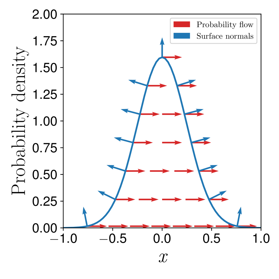
(a) $\mu$ flow lines

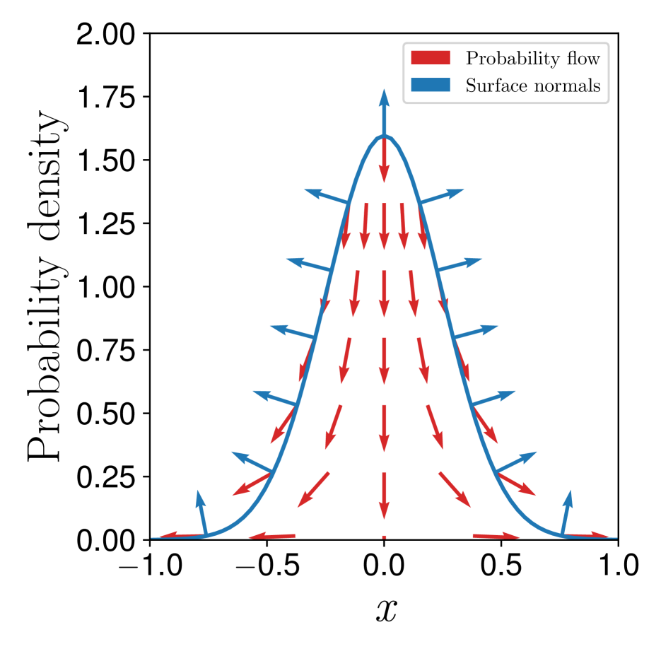
(b) $\sigma$ flow lines

Figure 3: Probability flow lines when $\mu$ and $\sigma$ are perturbed.

Here we give another explanation of LR and RP. In this theory, both LR and RP come out of the same derivation, thus showing a link between the two. In particular, we define an incompressible flow of probability mass imposed by perturbing the parameters $\theta$ of $p\left(x;\theta\right)$, which can be used to express the derivative of the expectation as an integral over this flow. LR and RP estimators correspond to duals of this integral under the well-known divergence theorem (Thm. 1).

The main idea resembles RP, but in addition to sampling ${\bm{x}}$, we sample a height $h$ for each point: $h~{}=~{}\epsilon_{h}p\left({\bm{x}};\theta\right)$, where $\epsilon_{h}\sim\textup{unif}(0,1)$, i.e., the sampling space is extended with an additional dimension for the height $\tilde{{\bm{x}}}:=[{\bm{x}}^{T},h]^{T}$, and we are uniformly sampling in the volume under $p\left({\bm{x}};\theta\right)$. The definition of $g$ in the introduction is extended, s.t. $\tilde{g}(\epsilon_{x},\epsilon_{h}):=\tilde{{\bm{x}}}=[g(\epsilon_{x})^{T},\epsilon_{h}p\left({\bm{x}};\theta\right)]^{T}$. The expectation turns into

$$\frac{\textup{d}\hfill}{\textup{d}\theta\hfill}\int p\left({\bm{x}};\theta\right)\phi({\bm{x}})\textup{d}{\bm{x}}$$ (16)

$$=\frac{\textup{d}\hfill}{\textup{d}\theta\hfill}\int_{\epsilon_{x}}\int_{\epsilon_{h}}p\left(\epsilon_{x}\right)p\left(\epsilon_{h}\right)\phi\left(\tilde{g}(\epsilon_{x},\epsilon_{h})\right)\textup{d}\epsilon_{x}\textup{d}\epsilon_{h}$$

$$=\int_{V}\nabla_{\theta}\phi(\tilde{g}(\epsilon_{x},\epsilon_{h}))\textup{d}V=\int_{V}\nabla_{\tilde{{\bm{x}}}}\phi(\tilde{{\bm{x}}})\nabla_{\theta}\tilde{g}(\epsilon_{x},\epsilon_{h})\textup{d}V.$$

In Eq. (16), $V$ is the volume under the curve of $p({\bm{x}};\theta)$, and $\phi([{\bm{x}}^{T},h]^{T})\coloneqq\phi({\bm{x}})$ ignores the $h$-component. Each column $i$ of $\nabla_{\theta}\tilde{g}(\epsilon_{x},\epsilon_{h})$ corresponds to a vector field induced by perturbing the $i^{\textup{th}}$ component of $\theta$. The red lines in Fig. 3 show the flow fields for a Gaussian distribution as the mean and variance are perturbed. The other term, $\nabla_{\tilde{{\bm{x}}}}\phi(\tilde{{\bm{x}}})$, is the gradient of the scalar field $\phi(\tilde{{\bm{x}}})$. As $\phi$ is independent of $h$, the gradient is parallel to the ${\bm{x}}$ axes with magnitude $\frac{\textup{d}\phi\hfill}{\textup{d}{\bm{x}}\hfill}$.

According to the divergence theorem in Eq. (13), the volume integral in Eq. (16) can be turned into a surface integral over the boundary ${\bm{S}}$ ($\textup{d}{\bm{S}}$ is a shorthand for $\hat{{\bm{n}}}\textup{d}S$, where $\hat{{\bm{n}}}$ is the surface normal vector), depicted by the blue lines in Fig. 3.

In Eq. (13), ${\bm{F}}$ is any vector field. A common corollary arises by picking ${\bm{F}}=\phi{\bm{v}}$, where $\phi$ is a scalar field, and ${\bm{v}}$ is a vector field. We choose ${\bm{v}}=\nabla_{\theta}\tilde{g}(\epsilon_{x},\epsilon_{h})\delta\theta$, where $\delta\theta$ is an arbitrary perturbation in $\theta$, so that ${\bm{F}}=\phi(\tilde{{\bm{x}}})\nabla_{\theta}\tilde{g}(\epsilon_{x},\epsilon_{h})\delta\theta$, in which case $\nabla_{\tilde{{\bm{x}}}}\cdot{\bm{F}}=\nabla_{\tilde{{\bm{x}}}}\cdot\left(\phi(\tilde{{\bm{x}}})\nabla_{\theta}\tilde{g}(\epsilon_{x},\epsilon_{h})\delta\theta\right)=\nabla_{\tilde{{\bm{x}}}}\phi(\tilde{{\bm{x}}})\nabla_{\theta}\tilde{g}(\epsilon_{x},\epsilon_{h})\delta\theta+\phi(\tilde{{\bm{x}}})\nabla_{\tilde{{\bm{x}}}}\cdot\nabla_{\theta}\tilde{g}(\epsilon_{x},\epsilon_{h})\delta\theta$. Note that the term $\nabla_{\theta}\tilde{g}(\epsilon_{x},\epsilon_{h})\delta\theta$ corresponds to an incompressible flow (because the probability density does not change at any point in the augmented space). As the divergence of an incompressible flow is 0, $\nabla_{\tilde{{\bm{x}}}}\cdot\nabla_{\theta}\tilde{g}(\epsilon_{x},\epsilon_{h})\delta\theta=0$, and the second term disappears. Noting that $\delta\theta$ can be canceled, because it is arbitrary, we are left with the equation:

$$\int_{V}\nabla_{\tilde{{\bm{x}}}}\phi(\tilde{{\bm{x}}})\nabla_{\theta}\tilde{g}(\epsilon_{x},\epsilon_{h})\textup{d}V =\int_{S}\phi(\tilde{{\bm{x}}})\nabla_{\theta}\tilde{g}(\epsilon_{x},\epsilon_{h})\cdot\textup{d}{\bm{S}}.$$ (17)

Now we explain how the left-hand side of Eq. (17) gives rise to the RP gradient estimator, while the right-hand side corresponds to the LR gradient estimator.

RP estimator:

Consider the $\nabla_{\tilde{{\bm{x}}}}\phi(\tilde{{\bm{x}}})\nabla_{\theta}\tilde{g}(\epsilon_{x},\epsilon_{h})$ term. As the scalar field $\phi(\tilde{{\bm{x}}})$ is independent of the height location $h$, the component of the gradient in that direction is 0, and $\nabla_{\tilde{{\bm{x}}}}\phi(\tilde{{\bm{x}}})=[\nabla_{{\bm{x}}}\phi({\bm{x}}),0]$. As the $h$-component is 0, the value of $\tilde{g}$ in the $h$-direction is multiplied by 0, and is irrelevant for the product, so $\nabla_{\tilde{{\bm{x}}}}\phi(\tilde{{\bm{x}}})\nabla_{\theta}\tilde{g}(\epsilon_{x},\epsilon_{h})=\nabla_{{\bm{x}}}\phi({\bm{x}})\nabla_{\theta}g(\epsilon_{x})$, which is just the term used in the RP estimator. Hence, the left-hand side of Eq. (17) corresponds to the RP gradient.

LR estimator:

We will show that the LR estimator tries to integrate $\int_{S}\phi(\tilde{{\bm{x}}})\nabla_{\theta}\tilde{g}(\epsilon_{x},\epsilon_{h})\cdot\textup{d}{\bm{S}}$. To do so, note that $\textup{d}{\bm{S}}=\hat{{\bm{n}}}\textup{d}S$. It is necessary to express the normalized surface vector $\hat{{\bm{n}}}$, and then perform the integral over the surface. The derivation is in App. D.2, and the final result is

$$\int_{S}\phi(\tilde{{\bm{x}}})\nabla_{\theta}\tilde{g}(\epsilon_{x},\epsilon_{h})\cdot\textup{d}{\bm{S}}=\int_{X}\phi({\bm{x}})\frac{\textup{d}p\left({\bm{x}};\theta\right)\hfill}{\textup{d}\theta\hfill}~{}\textup{d}{\bm{x}}.$$ (18)

We have already seen that MC integration of the right-hand side of Eq. (18) using samples from $p\left({\bm{x}};\theta\right)$ yields the LR estimator. Thus, RP and LR are duals under the divergence theorem. To further strengthen this claim we prove that the LR gradient estimator is the unique estimator that takes weighted averages of the function values $\phi({\bm{x}})$.

Theorem 2 (Uniqueness of LR estimator).

$\psi({\bm{x}})=p\left({\bm{x}};\theta\right)\frac{\textup{d}\log p\left({\bm{x}};\theta\right)\hfill}{\textup{d}\theta\hfill}$ is the unique function $\psi$, s.t. $\int\psi({\bm{x}})\phi({\bm{x}})\textup{d}{\bm{x}}=\frac{\textup{d}\hfill}{\textup{d}\theta\hfill}\int p\left({\bm{x}};\theta\right)\phi({\bm{x}})\textup{d}{\bm{x}}$ for all $\phi$.

Proof.

Suppose that there exist $\psi\neq f$, s.t. $\int\phi({\bm{x}})\psi({\bm{x}})~{}\textup{d}{\bm{x}}=\int\phi({\bm{x}})f({\bm{x}})~{}\textup{d}{\bm{x}}$ for all $\phi$. Rearrange the equation into $\int\phi({\bm{x}})\left(\psi({\bm{x}})-f({\bm{x}})\right)~{}\textup{d}{\bm{x}}=0$, then pick $\phi({\bm{x}})=\psi({\bm{x}})-f({\bm{x}})$ from which we get $\int\left(\psi({\bm{x}})-f({\bm{x}})\right)^{2}~{}\textup{d}{\bm{x}}=0$. This leads to $\psi=f$, which is a contradiction. Therefore, there cannot exist such $\psi\neq f$ that satisfy the condition for all $\phi$. ∎

The result also follows from the Riesz representation theorem (Riesz,, 1907). From the theorem, we see that Eq. (18) was immediately clear without having to go through the derivation in App. D.2. The same analysis does not work for RP (App. E.1). Indeed, there are infinitely many RP gradients (Jankowiak and Obermeyer,, 2018).

Characterizing the space of all LR and RP estimators:

Now we can derive a concrete form of all estimators in the abstract class in Eqs. (4) and (7). The flow theory assumed that the flow is aligned with the change of the probability density. We can lift this restriction by subtracting the excess probability mass (App. E.2), giving a general gradient estimator combining both $\phi({\bm{x}})$ and $\nabla_{{\bm{x}}}\phi({\bm{x}})$. This characterization is formalized in the theorem below.

Theorem 3 (The probability flow gradient estimator characterizes the space of all LR–RP gradient estimators).

Given a sample, ${\bm{x}}\sim q({\bm{x}})$, every unbiased gradient estimator, $E_{\theta_{i}}$, s.t. $\mathbb{E}_{q({\bm{x}})}\left[E_{\theta_{i}}\right]=\frac{\textup{d}\hfill}{\textup{d}\theta_{i}\hfill}\mathbb{E}_{p({\bm{x}};\theta)}\left[\phi({\bm{x}})\right]$, of the product form in Eq. (4),

$$E_{\theta_{i}}={\bm{v}}({\bm{x}})\cdot\nabla_{{\bm{x}}}\phi({\bm{x}})+\psi({\bm{x}})\phi({\bm{x}}),$$

where $\phi$ is an arbitrary function, and assuming $p({\bm{x}};\theta){\bm{v}}({\bm{x}})\phi({\bm{x}})\to 0$ as $\lVert x\rVert\to\infty$, is a special case of the estimator characterized by

$$E_{\theta_{i}}=\frac{p\left({\bm{x}};\theta\right)}{q\left({\bm{x}}\right)}{\bm{u}}_{\theta_{i}}({\bm{x}})\cdot\nabla_{{\bm{x}}}\phi({\bm{x}})$$ (19)

$$+\frac{1}{q\left({\bm{x}}\right)}\biggl{(}\nabla_{{\bm{x}}}\cdot\bigl{(}p\left({\bm{x}};\theta\right){\bm{u}}_{\theta_{i}}({\bm{x}})\bigr{)}+\frac{\textup{d}p\left({\bm{x}};\theta\right)\hfill}{\textup{d}\theta_{i}\hfill}\biggr{)}\phi({\bm{x}}),$$

where ${\bm{u}}_{\theta_{i}}$ is an arbitrary vector field. Note that, for simplicity, we also assumed continuity of $p$, $\phi$ and ${\bm{u}}_{\theta_{i}}$; however, this is unnecessary, and discontinuities are handled in App. E.4.

Proof.

It is analogous to Thm 2. See App. E.2.∎

The theorem says that given ${\bm{v}}$, one can derive the unique $\psi$ necessary for unbiasedness. Thus, the probability flow gradient in Eq. (19) generalizes all previous LR–RP gradients in the literature, as well as all possible gradient estimators having the product form in Eq. (4). By setting ${\bm{u}}_{\theta_{i}}({\bm{x}})={\bm{0}}$ one recovers LR; by setting $\nabla_{{\bm{x}}}\cdot\bigl{(}p\left({\bm{x}};\theta\right){\bm{u}}_{\theta_{i}}({\bm{x}})\bigr{)}+\frac{\textup{d}p\left({\bm{x}};\theta\right)\hfill}{\textup{d}\theta_{i}\hfill}=0$, one recovers the pathwise estimators described by Jankowiak and Obermeyer, (2018). Estimators combining both $\phi({\bm{x}})$ and $\nabla_{{\bm{x}}}\phi({\bm{x}})$, such as the generalized RP gradient (Ruiz et al., 2016b, ), also conform to Eq. (19) (App. E.3). Moreover, estimators in discontinuous situations, such as the GO gradient (Cong et al.,, 2019) or RP gradients for discontinuous models (Lee et al.,, 2018) also conform to this equation when taking into account for the discontinuities (App. E.4).

The terms in Eq. (19) can be readily interpreted. First note that $q({\bm{x}})$ is just a factor due to MC integration by sampling from $q$ (Sec. 2.3). The remaining terms can be made analogous to fluid motion. In the analogy, perturbing $\theta_{i}$ is equivalent to perturbing time measured in seconds (s), $p({\bm{x}};\theta)$ is equivalent to the density measured in $\frac{\textup{kg}\hfill}{\textup{m}^{3}}$, and ${\bm{u}}_{\theta_{i}}$ is equivalent to the flow velocity measured in $\frac{\textup{m}}{\textup{s}}$. The term, $p({\bm{x}};\theta){\bm{u}}_{\theta_{i}}({\bm{x}})$, is the probability mass flow rate per unit area, as is clear from multiplying the units: $\frac{\textup{kg}\hfill}{\textup{m}^{3}}\times\frac{\textup{m}}{\textup{s}}=\frac{\nicefrac{{\textup{kg}}}{{\textup{s}}}\hfill}{\textup{m}^{2}}$. The term $\nabla_{{\bm{x}}}\cdot\bigl{(}p\left({\bm{x}};\theta\right){\bm{u}}_{\theta_{i}}({\bm{x}})\bigr{)}$ is the divergence of the probability mass flow rate, and it tells us the rate of change of density at ${\bm{x}}$ with a corresponding $\phi({\bm{x}})$ caused by the probability flow, $p({\bm{x}};\theta){\bm{u}}_{\theta_{i}}({\bm{x}})$ (see Sec. 2.5). The $p\left({\bm{x}};\theta\right){\bm{u}}_{\theta_{i}}({\bm{x}})\cdot\nabla_{{\bm{x}}}\phi({\bm{x}})$ term, on the other hand, gives the rate of change of the $\phi({\bm{x}})$ corresponding to a point moving on the probability flow. Integrated across the whole volume, the two terms involving ${\bm{u}}_{\theta_{i}}$ cancel out, leaving only the $\frac{\textup{d}p({\bm{x}};\theta)\hfill}{\textup{d}\theta_{i}\hfill}$ term. The probability flow estimator could thus also be interpreted as adding a control variate to the standard LR gradient estimator.

Our explanation of the principle behind LR and RP gradients improves over previous explanations based on two main criteria: (i) greater generality, (ii) requiring fewer assumptions. In particular, Occam’s razor states that given competing explanations, one should prefer the one with fewer assumptions. Our explanation does not require the reparameterization assumption used in many previous explanations of RP gradients. Instead, we argue that reparameterization is just a trick that allows implementing the estimator easily using automatic differentiation, but has little to do with the principle behind its operation. Moreover, the sufficient conditions for the probability flow gradient estimator are also necessary, so the explanation of the principle cannot be improved without expanding the class of estimators to go beyond Eq. (4).

Our characterization showed that the flow field ${\bm{u}}_{\theta_{i}}({\bm{x}})$ and importance sampling distribution $q({\bm{x}})$, together, fully describe the space of estimators; one remaining question is how to pick ${\bm{u}}_{\theta_{i}}({\bm{x}})$ and $q({\bm{x}})$, s.t. the variance of the estimator is low. Jankowiak and Obermeyer, (2018) discussed how to pick ${\bm{u}}_{\theta_{i}}({\bm{x}})$ when the $\phi({\bm{x}})$ term disappears (i.e., for RP). In our concurrent work (Parmas and Sugiyama,, 2019), we are discussing how to pick $q({\bm{x}})$ when the $\nabla_{{\bm{x}}}\phi({\bm{x}})$ term disappears (i.e., for LR). The general question of the best combination of ${\bm{u}}_{\theta_{i}}({\bm{x}})$ and $q({\bm{x}})$ remains an open problem.

5 BENEFIT OF CHARACTERIZING THE SPACE OF ESTIMATORS

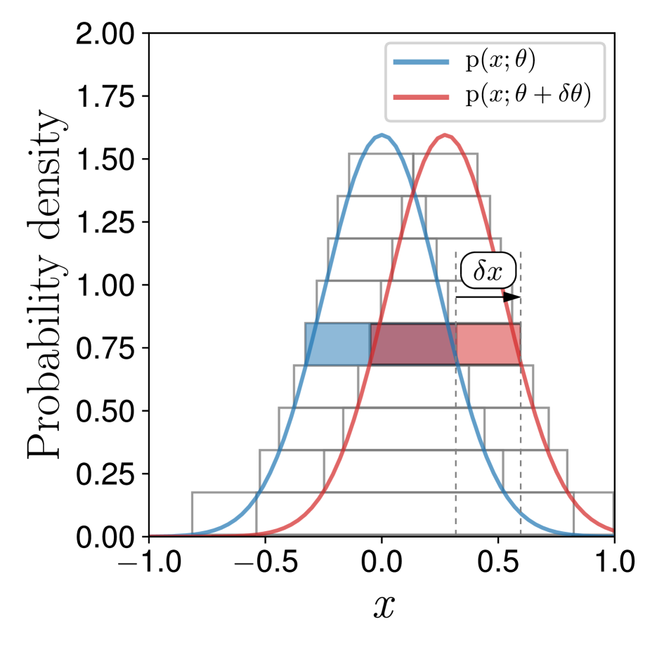
(a) Probability slices

(b) Probability density

Figure 4: Motivation for slice integral sampling and the importance distribution for a Gaussian base distribution.

Characterizing the space of estimators via uniqueness claims is highly useful because it clarifies where we should be searching for new gradient estimators. In particular, often a new idea might appear promising at first sight, but uniqueness claims could immediately say that the idea will not lead to something novel, and will instead be a special case of the characterized space. We illustrate this concept with two case studies below.

Case study 1 (Height reparameterization).

Consider the example with a height reparameterization explained in Sec. 4. After some derivations, we reached Eq. (17), which we repeat below:

$$\int_{V}\nabla_{\tilde{{\bm{x}}}}\phi(\tilde{{\bm{x}}})\nabla_{\theta}\tilde{g}(\epsilon_{x},\epsilon_{h})\textup{d}V =\int_{S}\phi(\tilde{{\bm{x}}})\nabla_{\theta}\tilde{g}(\epsilon_{x},\epsilon_{h})\cdot\textup{d}{\bm{S}}.$$

This equation looks promising because the left-hand side is known to correspond to RP, which is an unbiased gradient estimator. Therefore, we know that the right-hand side must also be unbiased, and it could potentially lead to some new interesting estimator using the $\phi({\bm{x}})$ information. However, to compute the estimator, we have to perform the tedious error-prone derivations in App. D.2. Instead, based on the uniqueness claim in Thm. 2 we can immediately say that this approach cannot possibly lead to a new estimator, because it has the same form as LR (product with $\phi({\bm{x}})$), saving us the trouble of going through the derivation.

Case study 2 (Horizontal slice integral sampling).

Consider an algorithm that would sample horizontal slices of probability mass, illustrated in Fig. 4(a), and motivated by flipping the vertical slices in Sec. 3. One could integrate the expectation over the slice, and try to estimate the gradient w.r.t. a parameter $\theta$.

Such an approach appears attractive, because if the location of the slice is moved by modifying the parameters of the distribution (e.g., by changing the mean, $\mu$), then the derivative of the expected value of the integral over the slice will depend only on the value at the edges of the slice (because the probability density in the middle would not change). To clarify, consider a uniform distribution $p(x;\mu)$ between $\mu\pm\Delta$. The derivative is $\frac{\textup{d}\hfill}{\textup{d}\mu\hfill}\int_{\mu-\Delta}^{\mu+\Delta}p(x;\mu)\phi(x)\textup{d}x=C\left(\phi(\mu+\Delta)-\phi(\mu-\Delta)\right)$, where $C$ is a constant. We could use importance sampling to sample on one of the two edges of the slice, to obtain an unbiased gradient estimator. However, at this point, it is clear that the estimator will belong to the same class as LR, as it will be averaging some value multiplied with $\phi(x)$, so we can already say that this idea is not promising. At best, it would lead to an LR gradient with a different sampling distribution $q(x)$—this is indeed the case, and the distribution is plotted in Fig. 4(b). The full derivation is in App. F.

Systematic approach to deriving estimators:

Rather than pursuing an ad hoc approach as in the two case studies, we propose that we should be using a more systematic approach in the search for new gradient estimators. It is not enough to find one novel estimator; one should find all estimators of a given novel class. Our proposed 3-step approach is below.

1. Find a new principle for a novel gradient estimator.
   In the case of LR and RP, the principle is to measure the movement of probability mass, as described in Sec. 3.

2. Parameterize the class of estimators that encloses all estimators embodying the said principle.
   In our case, this parameterization is in Eq. (4).

3. Find necessary and sufficient conditions for the estimator to be unbiased.
   In our case, these conditions were given in Sec. 4.

6 CONCLUSIONS

We introduced a complete unified theory of LR and RP gradients, and characterized the space of all unbiased single sample gradient estimators taking a weighted sum of $\phi({\bm{x}})$ and $\nabla_{{\bm{x}}}\phi({\bm{x}})$. Each estimator is defined by a vector field ${\bm{u}}_{\theta_{i}}({\bm{x}})$ and an importance sampling distribution $q({\bm{x}})$ that represent two “knobs” one can tune to improve gradient accuracy. We hope our work may lead to a systematic pursuit to characterizing all possible gradient estimators based on different principles of Monte Carlo gradient estimation.

Acknowledgements

PP was supported by KAKENHI Grants 16H06561, 16H06563 and 16K21738, by the research support of the Okinawa Institute of Science and Technology Graduate University for the Neural Computation Unit, by RIKEN during an internship, and by the Cyborg-AI project supported by NEDO, Japan. MS was supported by KAKENHI 17H00757.

 

A unified view of likelihood ratio and reparameterization gradients:
Supplementary Materials

 

[sections] [sections]l1

Appendix A Additional background literature on LR and RP

See the work by Mohamed et al., (2019) for a recent extensive general review of Monte Carlo gradient estimators, such as LR and RP. Here we discuss the main points about LR and RP in the literature, and how these are related to our work.

Advantages and disadvantages of LR and RP:

The variance of LR and RP gradients has been of central importance in their research. Typically, RP is said to be more accurate and scale better with the sampling dimension (Rezende et al.,, 2014)—this claim is also backed by theory (Xu et al.,, 2019; Nesterov and Spokoiny,, 2017); however, there is no guarantee that RP outperforms LR. In particular, for multimodal $\phi(x)$ (Gal,, 2016) or chaotic systems (Parmas et al.,, 2018), LR can be arbitrarily better than RP (e.g., the latter showed that LR can be $10^{6}$ more accurate in practice). Moreover, RP is not directly applicable to discrete sampling spaces, but requires continuous relaxations (Maddison et al.,, 2016; Jang et al.,, 2016; Tucker et al.,, 2017). Differentiable RP is also not always possible, but implicit RP gradients have increased the number of usable distributions (Figurnov et al.,, 2018). Because LR and RP both have advantages and disadvantages, optimal estimation techniques will require a combination of LR and RP as considered in the flow gradients.

Variance reduction techniques:

Techniques for variance reduction have been extensively studied, including control variates/baselines (Grathwohl et al.,, 2017; Greensmith et al., 2004b, ; Tucker et al.,, 2018; Gu et al.,, 2015; Geffner and Domke,, 2018; Gu et al.,, 2016) as well as Rao-Blackwellization (Titsias and Lázaro-Gredilla,, 2015; Ciosek and Whiteson,, 2018; Asadi et al.,, 2017). One can also combine the best of both LR and RP gradients by dynamically reweighting them (Parmas et al.,, 2018; Metz et al.,, 2019).

LR and RP on computational graphs:

Several methods for computing LR and RP gradients on graphs of computations exist (Schulman et al., 2015a, ; Weber et al.,, 2019; Parmas,, 2018; Foerster et al.,, 2018; Mao et al.,, 2019; Farquhar et al.,, 2019). Among these works, Schulman et al., 2015a provided a simple way to obtain the gradient estimators using automatic differentiation of a surrogate objective on stochastic computation graphs; Weber et al., (2019) extended this work to be also applicable for gradient estimators using critics; Parmas, (2018) provided an intuitive abstract framework for reasoning about gradient estimators by turning the stochastic graph deterministic through considering gradients of the marginal distributions w.r.t. the distributions at the other nodes, thus allowing to apply the total derivative rule; Foerster et al., (2018) extended the surrogate loss concept for higher order derivatives; Mao et al., (2019) provided a baseline for higher order LR estimators, and Farquhar et al., (2019) derived a way to trade off bias and variance.

Importance sampling:

Importance sampling for reducing LR gradient variance was previously considered in variational inference (Ruiz et al., 2016a, ), who proposed to sample from the same distribution while tuning the variance. In reinforcement learning, importance sampling has been studied for sample reuse via off-policy policy evaluation (Thomas and Brunskill,, 2016; Jiang and Li,, 2016; Gu et al.,, 2017; Munos et al.,, 2016; Jie and Abbeel,, 2010), but modifying the policy to improve gradient accuracy has not been considered.

Other:

The flow theory in Sec. 4 was concurrently derived by (Jankowiak and Obermeyer,, 2018), but their work focused on deriving new RP gradient estimators, and they do not discuss the duality. Our derivation is also more visual. We discuss the relationship between their work and ours in more detail in App. E.2. The flow gradient estimator in Eq. (19) was also presented in a work in progress by Wu, (2019) slightly earlier, but in their derivation they do not use the divergence theorem, and assume that ${\bm{u}}_{\theta_{i}}({\bm{x}})$ belongs to a reparameterizable variable, whereas we do not make such an assumption, and argue that the flow is a more fundamental concept than the reparameterization of the variable. An advantage of their work is that they show a new polynomial-based gradient estimator, whereas we focus on characterizing the space of estimators. One point is that there always exists a flow corresponding to a reparameterization; however, it is an open question whether there exists a reparameterization corresponding to each flow ${\bm{u}}_{\theta_{i}}({\bm{x}})$. Our main contribution regarding this estimator is the discussion around it, which claims that the flow ${\bm{u}}_{\theta_{i}}({\bm{x}})$ is a fundamental concept that characterizes the space of all possible single sample estimators, as well as the visualizations and physical intuitions that we provide.

Appendix B Likelihood ratio gradient basics

The likelihood ratio (LR) gradient estimator is given by

$$\frac{\textup{d}\hfill}{\textup{d}\theta\hfill}\mathbb{E}_{x\sim p\left(x;\theta\right)}\left[\phi(x)\right]=\mathbb{E}_{x\sim p\left(x;\theta\right)}\left[\frac{\textup{d}\log p\left(x;\theta\right)\hfill}{\textup{d}\theta\hfill}\phi(x)\right].$$ (20)

For a Gaussian $p\left(x;\theta\right)$:

$$\log p\left(x;\theta\right) =-\frac{1}{2}\log(2\pi)-\log(\sigma)-\frac{(x-\mu)^{2}}{2\sigma^{2}},$$ (21)

$$\frac{\textup{d}\log p\left(x;\theta\right)\hfill}{\textup{d}\mu\hfill} =\frac{x-\mu}{\sigma^{2}}=\frac{\epsilon}{\sigma},$$

$$\frac{\textup{d}\log p\left(x;\theta\right)\hfill}{\textup{d}\sigma\hfill} =\frac{(x-\mu)^{2}}{\sigma^{3}}-\frac{1}{\sigma}=\frac{\epsilon^{2}}{\sigma}-\frac{1}{\sigma},$$

where $$x=\mu+\epsilon\sigma\textup{ and }\epsilon\sim\mathcal{N}(0,1).$$

Baselines to reduce gradient variance:

The LR gradient estimator on its own has a large variance, and techniques have to be used to stabilize it. A common technique is to subtract a constant baseline $b$ from the $\phi(x)$ values, so that the gradient estimator becomes

$$\frac{\textup{d}\hfill}{\textup{d}\theta\hfill}\mathbb{E}_{x\sim p\left(x;\theta\right)}\left[\frac{\textup{d}\log p\left(x;\theta\right)\hfill}{\textup{d}\theta\hfill}\left(\phi(x)-b\right)\right].$$ (22)

In practice, using $b=\mathbb{E}_{x\sim p\left(x;\theta\right)}\left[\phi(x)\right]$ works well, but one can also derive an optimal baseline (Weaver and Tao,, 2001). We outline the derivation below. The gradient variance when a baseline is used can be expressed as

$$\mathbb{V}_{x\sim p\left(x;\theta\right)}\left[\frac{\textup{d}\log p\left(x;\theta\right)\hfill}{\textup{d}\theta\hfill}\left(\phi(x)-b\right)\right] =~{}~{}\mathbb{E}_{x\sim p\left(x;\theta\right)}\left[\left(\frac{\textup{d}\log p\left(x;\theta\right)\hfill}{\textup{d}\theta\hfill}\phi(x)\right)^{2}\right]$$ (23)

$$-2\mathbb{E}_{x\sim p\left(x;\theta\right)}\left[\left(\frac{\textup{d}\log p\left(x;\theta\right)\hfill}{\textup{d}\theta\hfill}\right)^{2}\phi(x)b\right]$$

$$+\mathbb{E}_{x\sim p\left(x;\theta\right)}\left[\left(\frac{\textup{d}\log p\left(x;\theta\right)\hfill}{\textup{d}\theta\hfill}b\right)^{2}\right].$$

Taking the derivative of Eq. (23) w.r.t. $b$ and setting to zero gives the optimal baseline as

$$b_{opt}=\frac{\mathbb{E}_{x\sim p\left(x;\theta\right)}\left[\left(\frac{\textup{d}\log p\left(x;\theta\right)\hfill}{\textup{d}\theta\hfill}\right)^{2}\phi(x)\right]}{\mathbb{E}_{x\sim p\left(x;\theta\right)}\left[\left(\frac{\textup{d}\log p\left(x;\theta\right)\hfill}{\textup{d}\theta\hfill}\right)^{2}\right]}.$$ (24)

In practice, for example if $\phi(x)$ is linear and $p\left(x;\theta\right)$ is Gaussian then $b_{opt}=\mathbb{E}_{x\sim p\left(x;\theta\right)}\left[\phi(x)\right]$, so the gain from trying to use an optimal baseline is often small.

Antithetic sampling:

An often used technique is to sample points $x$ in pairs opposite to each other, s.t. $x_{+}=\mu+\sigma\epsilon$ and $x_{-}=\mu-\sigma\epsilon$. This technique is particularly often used in evolution strategies’ research (Salimans et al.,, 2017; Mania et al.,, 2018). We will explain that when this technique is used, then a baseline has no effect because it cancels. The derivation is easy to see by considering that for a Gaussian: $\frac{\textup{d}\log p\left(x;\theta\right)\hfill}{\textup{d}\mu\hfill}=\frac{\epsilon}{\sigma}$, so

$$\frac{\textup{d}\log p\left(x_{+};\theta\right)\hfill}{\textup{d}\mu\hfill}(\phi(x_{+})-b)+\frac{\textup{d}\log p\left(x_{-};\theta\right)\hfill}{\textup{d}\mu\hfill}(\phi(x_{-})-b)$$

$$=\frac{\epsilon}{\sigma}\left(\phi(x_{+})-b-(\phi(x_{-})-b)\right)=\frac{\epsilon}{\sigma}\left(\phi(x_{+})-\phi(x_{-})\right).$$

Relationship to finite difference methods:

Finite difference methods also use the function values $\phi(x)$ to estimate a derivative, so it may appear that the LR gradient estimator is a finite difference estimator. Finite difference estimators work by estimating the slope of the function, by evaluating the change between two points, i.e.

$$\frac{\textup{d}\phi(x)\hfill}{\textup{d}x\hfill}\approx\frac{\phi(x_{+})-\phi(x_{-})}{\Delta x}.$$ (25)

In the antithetic sampling case, $\Delta x=2\sigma\epsilon$, so the estimator is

$$\frac{\textup{d}\phi(x)\hfill}{\textup{d}x\hfill}\approx\frac{\phi(x_{+})-\phi(x_{-})}{2\sigma\epsilon}.$$ (26)

Clearly, this is different to the LR gradient estimator averaged over one pair of samples $\frac{1}{2}\left(\frac{\epsilon}{\sigma}\phi(x_{+})+\frac{-\epsilon}{\sigma}\phi(x_{-})\right)$:

$$\frac{\epsilon\left(\phi(x_{+})-\phi(x_{-})\right)}{2\sigma},$$ (27)

because the $\epsilon$ is in the wrong place. In Sec. 3 we explain that the LR gradient estimator is a different concept to finite differences, which is not trying to fit a linear function onto $\phi(x)$.

Appendix C Probability boxes formal derivation

Here we give a more formal derivation of the “probability boxes” explanation in Sec. 3. In the theory, we explained that the expectation can be written as a weighted average $\sum_{i=1}^{N}P(x_{i})\phi(x_{i})$ of function values, where the weight is given by the probabilities. Then, the LR gradient estimated the derivative of this expectation w.r.t. $\theta$ by differentiating the $P(x_{i})$ term, whereas the RP gradient worked by differentiating the $\phi(x_{i})$ term. In this section, we will formally define the locations and edges of the “boxes” when a continuous integral is discretized, and show that in the LR case, indeed $\phi(x_{i})$ in the “box” stays fixed, whereas in the RP case, indeed the probability mass $P(x_{i})$ in the “box” stays fixed as the parameters $\theta$ are perturbed.

The explanation relies on a first principles thinking about the effect that changing the parameters of a probability distribution $\theta$ has on infinitesimal “boxes” of probability mass (Fig. 2). Both LR and RP are trying to estimate

$$\frac{\textup{d}\hfill}{\textup{d}\theta\hfill}\int p\left(x;\theta\right)\phi(x)\textup{d}x.$$ (28)

A typical finite explanation of Riemann integrals is performed by discretizing the integrand into “boxes” of size $\Delta x$, and summing:

$$\frac{\textup{d}\hfill}{\textup{d}\theta\hfill}\sum_{i=1}^{N}p\left(x_{i};\theta\right)\Delta x_{i}\phi(x_{i}).$$ (29)

Taking the limit as $N\rightarrow\infty$ recovers the true integral. In this equation, $P(x_{i})=p\left(x_{i};\theta\right)\Delta x_{i}$ is the amount of probability mass inside the “box”, and $\phi(x_{i})$ is the function value inside the “box”.

RP estimator:

Such a view can be used to explain RP gradients. In this case, the boundaries of the “box” are fixed with reference to the shape of the probability distribution, i.e. for each $i$ we define the center of the box as

$$x_{i}=g(\epsilon_{i};\theta),$$ (30)

and the boundaries as

$$g(\epsilon_{i}\pm\Delta\epsilon/2;\theta),$$ (31)

where $\epsilon_{i}$ is the reference position on a fixed simple distribution, $p\left(\epsilon\right)$. The amount of probability mass assigned to each “box” stays fixed at

$$P_{i}=p\left(\epsilon\right)\Delta\epsilon~{};$$ (32)

however, the center of the “box” moves, so the function value $\phi(x_{i})$ inside each “box” changes by

$$\delta\phi_{i}=\phi\left(g(\epsilon_{i};\theta+\delta\theta)\right)~{}-~{}\phi\left(g(\epsilon_{i};\theta)\right)=\phi(x_{i}~{}+~{}\delta x_{i})~{}-~{}\phi(x_{i}).$$ (33)

The full derivative can then be expressed as

$$\frac{\textup{d}\hfill}{\textup{d}\theta\hfill}\mathbb{E}_{x\sim p\left(x;\theta\right)}\left[\phi(x)\right]\approx\frac{1}{\delta\theta}\sum_{i=1}^{N}P_{i}\delta\phi_{i}=\sum_{i=1}^{N}P_{i}\frac{\delta\phi_{i}}{\delta x_{i}}\frac{\delta x_{i}}{\delta\theta}.$$ (34)

Taking the infinitesimal limit $N\rightarrow\infty$, and noting $P_{i}=p\left(x_{i};\theta\right)\Delta x_{i}$, we obtain the RP estimator

$$\int p\left(x;\theta\right)\frac{\textup{d}\phi(x)\hfill}{\textup{d}x\hfill}\frac{\textup{d}x\hfill}{\textup{d}\theta\hfill}~{}\textup{d}x.$$ (35)

We see that RP essentially estimates the gradient by keeping the probability mass inside each “box” fixed, but estimating how the function value $\phi$ inside the “box” changes as the parameters $\theta$ are perturbed.

LR estimator:

The LR gradient, on the other hand, keeps the boundaries of the “boxes” fixed, i.e. the center of the box is at $x_{i}$, and the boundaries at

$$x_{i}\pm\Delta x_{i}/2.$$ (36)

Now, as the boundaries are independent of $\theta$, the function value $\phi(x_{i})$ inside the box stays fixed, even as $\theta$ is perturbed by $\delta\theta$; however, the probability mass inside the box changes, because the density changes by

$$\delta p_{i}=p\left(x_{i};\theta+\delta\theta\right)-p\left(x_{i};\theta\right).$$ (37)

The full derivative can be expressed as

$$\frac{\textup{d}\hfill}{\textup{d}\theta\hfill}\mathbb{E}_{x\sim p\left(x;\theta\right)}\left[\phi(x)\right]\approx\frac{1}{\delta\theta}\sum_{i=1}^{N}\Delta x_{i}\delta p_{i}\phi(x_{i})=\sum_{i=1}^{N}p\left(x_{i};\theta\right)\Delta x_{i}\frac{\delta p_{i}/\delta\theta}{p\left(x_{i};\theta\right)}\phi(x_{i}).$$ (38)

Where we have multiplied and divided by $p\left(x_{i};\theta\right)$. Taking the infinitesimal limit recovers the LR gradient

$$\int p\left(x;\theta\right)\frac{\frac{\textup{d}p\left(x;\theta\right)\hfill}{\textup{d}\theta\hfill}}{p\left(x;\theta\right)}\phi(x)~{}\textup{d}x=\mathbb{E}_{x\sim p\left(x;\theta\right)}\left[\frac{\frac{\textup{d}p\left(x;\theta\right)\hfill}{\textup{d}\theta\hfill}}{p\left(x;\theta\right)}\phi(x)\right].$$ (39)

The transformation

$$p\left(x;\theta\right)\frac{\frac{\textup{d}p\left(x;\theta\right)\hfill}{\textup{d}\theta\hfill}}{p\left(x;\theta\right)}=p\left(x;\theta\right)\frac{\textup{d}\log p\left(x;\theta\right)\hfill}{\textup{d}\theta\hfill}$$ (40)

is known as the log-derivative trick, and it may appear to be the essence behind the LR gradient, but actually the multiplication and division by $p(x;\theta)$ is just a special case of the more general Monte Carlo integration principle. Any integral $\int f(x)~{}\textup{d}x$ can be approximated by sampling from a distribution $q(x)$ as

$$\int f(x)~{}\textup{d}x=\int q(x)\frac{f(x)}{q(x)}~{}\textup{d}x=\mathbb{E}_{x\sim q(x)}\left[\frac{f(x)}{q(x)}\right].$$ (41)

Rather than thinking of the LR gradient in terms of the log-derivative term, it may be better to think of it as simply estimating the integral $\int\frac{\textup{d}p\left(x;\theta\right)\hfill}{\textup{d}\theta\hfill}\phi(x)~{}\textup{d}x$ by applying the appropriate importance weights to samples from $p(x;\theta)$. Thus, we see that in the discretized case, the LR gradient picks $q(x)=p\left(x;\theta\right)$ (Jie and Abbeel,, 2010) and performs Monte Carlo integration to approximate $\frac{1}{\delta\theta}\sum_{i=1}^{N}\Delta x_{i}\delta p_{i}\phi(x_{i})$ by sampling from $P(x_{i})=\Delta x_{i}p\left(x_{i};\theta\right)$. To summarize: LR estimates the gradient by keeping the boundaries of the boxes fixed, measuring the change in probability mass in each box, and weighting by the function value: $\phi(x_{i})\delta p$.

Sometimes, the LR gradient is described as being “kind of like a finite difference gradient” (Salimans et al.,, 2017; Mania et al.,, 2018), but here we see that it is a different concept, which does not rely on fitting a straight line between differences of $\phi$ (App. B), but estimates how probability mass is reallocated among different $\phi$ values via Monte Carlo integration by sampling from $p\left(x;\theta\right)$.

Appendix D Derivations for the probability flow theory

(The notation and divergence theorem proof are the same as in the main paper, and provided here for reference.) We illustrate the background information in 3 dimensions, but it generalizes straightforwardly to higher dimensions.

Notation:

${\bm{F}}=[F_{x}(x,y,z),F_{y}(x,y,z),F_{z}(x,y,z)]$ is a vector field.
$\phi(x,y,z)$ is a scalar field (a scalar function).
Div operator: $\nabla\cdot{\bm{F}}=\frac{\partial F_{x}\hfill}{\partial x\hfill}+\frac{\partial F_{y}\hfill}{\partial y\hfill}+\frac{\partial F_{z}\hfill}{\partial z\hfill}$.
Grad operator: $\nabla\phi=[\frac{\partial\phi\hfill}{\partial x\hfill},\frac{\partial\phi\hfill}{\partial y\hfill},\frac{\partial\phi\hfill}{\partial z\hfill}]$.

D.1 Basic vector calculus and fluid mechanics

Figure 5: Illustration of the divergence theorem.

The vector field ${\bm{F}}$ could be for example thought of as a local flow velocity for some fluid. If ${\bm{F}}$ is the density flow rate, then the div operator essentially measures how much the density is decreasing at a point. If the outflow is larger than the inflow, the density would decrease and vice versa. The divergence theorem, illustrated in Fig. 5 illustrates how this change in density can be measured in two separate ways: one could integrate the divergence across the volume, or one could integrate the inflow and outflow across the surface. The divergence theorem states:

$$\int_{V}\nabla\cdot{\bm{F}}\textup{d}V=\int_{S}{\bm{F}}\cdot\textup{d}{\bm{S}}.$$ (42)

To prove the claim, consider the infinitesimal box in Fig. 5. The divergence can be calculated as $\delta x\delta y(\frac{\partial F_{x}\hfill}{\partial x\hfill}+\frac{\partial F_{y}\hfill}{\partial y\hfill})$. On the other hand, to take the integral across the surface, note that the surface normals point outwards, and the integral becomes $\delta_{y}(-F_{x}+F_{x}-\frac{\partial F_{x}\hfill}{\partial x\hfill}\delta x)+\delta x(-F_{y}+F_{y}+\frac{\partial F_{y}\hfill}{\partial y\hfill}\delta y)=\delta x\delta y(\frac{\partial F_{x}\hfill}{\partial x\hfill}+\frac{\partial F_{y}\hfill}{\partial y\hfill})$, which is the same as the divergence. To generalize this to arbitrarily large volumes, notice that if one stacks the boxes next to each other, then the surface integral across the area where the boxes meet cancels out, and only the integral across the outer surface remains. For an incompressible flow, the density does not change, and the divergence must be zero.

D.2 Derivation of probability surface integral

We will show that the LR estimator tries to integrate $\int_{S}\phi(\tilde{{\bm{x}}})\nabla_{\theta}\tilde{g}(\epsilon_{x},\epsilon_{h})\textup{d}{\bm{S}}$. First, note that $\textup{d}{\bm{S}}=\hat{{\bm{n}}}\textup{d}S$, and it is necessary to express the normalized surface vector $\hat{{\bm{n}}}$. To do so, we first express the tangent vectors ${\bm{t}}$, then find the vector perpendicular to all of them (this is exactly the normal vector).

All tangent vectors are characterized by the equation ${\bm{t}}=\left[{\bm{r}},\frac{\textup{d}p\hfill}{\textup{d}{\bm{x}}\hfill}\cdot{\bm{r}}\right]$, where ${\bm{r}}$ is an arbitrary vector. The normal vector ${\bm{n}}$ is such that ${\bm{t}}\cdot{\bm{n}}=0$ for all tangent vectors. Therefore, the normal vector ${\bm{n}}=\left[-\frac{\textup{d}p\hfill}{\textup{d}{\bm{x}}\hfill},1\right]$, satisfies the equation, because ${\bm{n}}\cdot{\bm{t}}=-\frac{\textup{d}p\hfill}{\textup{d}{\bm{x}}\hfill}\cdot{\bm{r}}+1\cdot\frac{\textup{d}p\hfill}{\textup{d}{\bm{x}}\hfill}\cdot{\bm{r}}=0$. Finally, we normalize the vector:

$$\hat{{\bm{n}}}=\nicefrac{{\left[-\frac{\textup{d}p\hfill}{\textup{d}{\bm{x}}\hfill},1\right]}}{{\sqrt{\left(\frac{\textup{d}p\hfill}{\textup{d}{\bm{x}}\hfill}\right)\left(\frac{\textup{d}p\hfill}{\textup{d}{\bm{x}}\hfill}\right)^{T}+1}}}~{}.$$ (43)

Next, we perform a change of coordinates from the surface elements $\textup{d}S$ to cartesian coordinates $\textup{d}{\bm{x}}$. When projecting a surface element $\textup{d}S$ with unit normal $\hat{{\bm{n}}}$ to a plane with unit normal $\hat{{\bm{m}}}$, the projected area is given by $\textup{d}{\bm{x}}=\left|\hat{{\bm{n}}}\cdot\hat{{\bm{m}}}\right|\textup{d}S$, therefore, as $\hat{{\bm{m}}}=[{\bm{0}},1]$ for the ${\bm{x}}$-plane, we have $\textup{d}{\bm{x}}~{}=~{}\textup{d}S\left|\frac{1}{\sqrt{\left(\frac{\textup{d}p\hfill}{\textup{d}{\bm{x}}\hfill}\right)\left(\frac{\textup{d}p\hfill}{\textup{d}{\bm{x}}\hfill}\right)^{T}+1}}\left[-\frac{\textup{d}p\hfill}{\textup{d}{\bm{x}}\hfill},1\right]\cdot[{\bm{0}},1]\right|=\nicefrac{{\textup{d}S}}{{\sqrt{\left(\frac{\textup{d}p\hfill}{\textup{d}{\bm{x}}\hfill}\right)\left(\frac{\textup{d}p\hfill}{\textup{d}{\bm{x}}\hfill}\right)^{T}+1}}}$, which leads to

$$\textup{d}S=\sqrt{\left(\frac{\textup{d}p\hfill}{\textup{d}{\bm{x}}\hfill}\right)\left(\frac{\textup{d}p\hfill}{\textup{d}{\bm{x}}\hfill}\right)^{T}+1}~{}~{}\textup{d}{\bm{x}}.$$ (44)

Plugging Eqs. (43) and (44) into the right-hand side of Eq. (17) we get

$$\int_{X}\phi(\tilde{{\bm{x}}})\nabla_{\theta}\tilde{g}(\epsilon_{x},\epsilon_{h})\cdot\frac{\left[-\frac{\textup{d}p\hfill}{\textup{d}{\bm{x}}\hfill},1\right]}{\sqrt{\left(\frac{\textup{d}p\hfill}{\textup{d}{\bm{x}}\hfill}\right)\left(\frac{\textup{d}p\hfill}{\textup{d}{\bm{x}}\hfill}\right)^{T}+1}}\sqrt{\left(\frac{\textup{d}p\hfill}{\textup{d}{\bm{x}}\hfill}\right)\left(\frac{\textup{d}p\hfill}{\textup{d}{\bm{x}}\hfill}\right)^{T}+1}~{}~{}\textup{d}{\bm{x}}=\int_{X}\phi(\tilde{{\bm{x}}})\nabla_{\theta}\tilde{g}(\epsilon_{x},\epsilon_{h})\cdot\left[-\frac{\textup{d}p\hfill}{\textup{d}{\bm{x}}\hfill},1\right]~{}\textup{d}{\bm{x}}.$$ (45)

Recall that the last element of $\tilde{g}(\epsilon_{x},\epsilon_{h})$ is $\epsilon_{h}p\left(g(\epsilon_{x});\theta\right)$, and that at the boundary surface $\epsilon_{h}=1$, then the scalar product term $\nabla_{\theta}\tilde{g}(\epsilon_{x},\epsilon_{h})\cdot\left[-\frac{\textup{d}p\hfill}{\textup{d}{\bm{x}}\hfill},1\right]$ turns into $-\nabla_{\theta}g(\epsilon_{x})\cdot\frac{\textup{d}p\hfill}{\textup{d}{\bm{x}}\hfill}+\left.\frac{\partial\epsilon_{h}p\left(g(\epsilon_{x});\theta\right)\hfill}{\partial\theta\hfill}\right|_{\epsilon_{x}=const,\epsilon_{h}=1}$. The last term $\left.\frac{\partial p\left(g(\epsilon_{x});\theta\right)\hfill}{\partial\theta\hfill}\right|_{\epsilon_{x}=const}$ can be thought of as the rate of change of the probability density while following a point moving in the flow induced by perturbing $\theta$. This quantity can be expressed with the material derivative $\left.\frac{\partial p\left(g(\epsilon_{x});\theta\right)\hfill}{\partial\theta\hfill}\right|_{\epsilon_{x}=const}=\frac{\textup{d}p\left({\bm{x}};\theta\right)\hfill}{\textup{d}\theta\hfill}+\nabla_{\theta}g(\epsilon_{x})\cdot\frac{\textup{d}p\hfill}{\textup{d}{\bm{x}}\hfill}$. Finally, substituting into Eq. (45):

$$\int_{S}\phi(\tilde{{\bm{x}}})\nabla_{\theta}\tilde{g}(\epsilon_{x},\epsilon_{h})~{}\textup{d}{\bm{S}}=\int_{X}\phi({\bm{x}})\frac{\textup{d}p\left({\bm{x}};\theta\right)\hfill}{\textup{d}\theta\hfill}~{}\textup{d}{\bm{x}}.$$ (46)

Appendix E Characterizing the space of all likelihood ratio and reparameterization gradients

E.1 Reparameterization gradients are not unique

What happens if we perform the same kind of analysis as in Theorem 2 for the RP gradient? To examine this idea, first we extend the argumentation in the main paper to include non-invertible $g(\epsilon;\theta)$, i.e., consider the case when multiple different $\epsilon$ lead to the same $x$ via $x=g(\epsilon;\theta)$. In Sec. 2.2 we argued that if $g$ is invertible, we can write the RP gradient as $\frac{\textup{d}\phi(x)\hfill}{\textup{d}x\hfill}\left.\frac{\partial g(\epsilon;\theta)\hfill}{\partial\theta\hfill}\right|_{\epsilon=S(x;\theta)}$, where $\left.\frac{\partial g(\epsilon;\theta)\hfill}{\partial\theta_{i}\hfill}\right|_{\epsilon=S(x;\theta)}$ corresponds to ${\bm{u}}_{\theta_{i}}({\bm{x}})$, which is a vector field. In the non-invertible case, similarly denote $S(x;\theta)$ is the set of $\epsilon$, s.t. $x=g(\epsilon;\theta)$. For each x, we can employ Bayes’ rule to derive the posterior distribution of the $\epsilon$ that generated $x$, and integrate across this distribution to obtain the Rao-Blackwellized estimator $\frac{\textup{d}\phi(x)\hfill}{\textup{d}x\hfill}\left.\int_{S(x;\theta)}p(\epsilon)\left.\frac{\partial g(\epsilon;\theta)\hfill}{\partial\theta\hfill}\right|_{\epsilon\in S(x;\theta)}\textup{d}\epsilon\middle/\int_{S(x;\theta)}p(\epsilon)\textup{d}\epsilon\right.$, where $\left.\int_{S(x;\theta)}p(\epsilon)\left.\frac{\partial g(\epsilon;\theta)\hfill}{\partial\theta_{i}\hfill}\right|_{\epsilon\in S(x;\theta)}\textup{d}\epsilon\middle/\int_{S(x;\theta)}p(\epsilon)\textup{d}\epsilon\right.$ corresponds to ${\bm{u}}_{\theta_{i}}({\bm{x}})$, which is a vector field. Thus, even in the non-invertible case, the reparameterization gradient can be expressed as a dot product between $\nabla_{{\bm{x}}}\phi({\bm{x}})$ and a vector field ${\bm{u}}({\bm{x}})$.

Now we show that the type of analysis in Thm. 2 does not lead to a uniqueness claim for RP gradients. Similarly, suppose that there exist ${\bm{u}}({\bm{x}})$ and ${\bm{v}}({\bm{x}})$, s.t. $\int\nabla\phi({\bm{x}})\cdot{\bm{u}}({\bm{x}})~{}\textup{d}{\bm{x}}=\int\nabla\phi({\bm{x}})\cdot{\bm{v}}({\bm{x}})~{}\textup{d}{\bm{x}}$ for any $\phi({\bm{x}})$. Rearrange the equation into $\int\nabla\phi({\bm{x}})\cdot\left({\bm{u}}({\bm{x}})-{\bm{v}}({\bm{x}})\right)~{}\textup{d}{\bm{x}}=0$. Then, if we can pick $\nabla\phi({\bm{x}})={\bm{u}}({\bm{x}})-{\bm{v}}({\bm{x}})$ it would lead to ${\bm{u}}={\bm{v}}$, which would show the uniqueness. In the one-dimensional case, this is possible, and in this case all pure reparameterization or pathwise gradients are equivalent. However, in higher dimensions, it is not necessarily possible to pick such $\phi({\bm{x}})$. In particular, the integral of $\nabla\phi({\bm{x}})$ over any closed path is 0, but this is not necessarily the case for ${\bm{u}}-{\bm{v}}$. Therefore, the same kind of analysis does not lead to a claim of uniqueness. Indeed, concurrent work (Jankowiak and Obermeyer,, 2018) showed that there are an infinite amount of possible reparameterization gradients, and the minimum variance is achieved by the optimal transport flow.

E.2 Flow gradient estimator

In this section, we provide the derivations and proofs for the flow gradient estimator in Eq. (19). While our derivation with a height reparameterization in Sec. 4 shows the duality between LR and RP, and allows for intuitive visualizations, the method of derivations by Jankowiak and Obermeyer, (2018) is algebraically easier to work with, so we adopt their style in the following sections. Recall the divergence theorem $\int_{V}\nabla_{{\bm{x}}}\cdot{\bm{F}}\textup{d}V=\int_{S}{\bm{F}}\cdot\textup{d}{\bm{S}},$ where ${\bm{F}}$ is an arbitrary continuous piecewise differentiable vector field. We can pick ${\bm{F}}=p\left({\bm{x}};\theta\right){\bm{u}}_{\theta_{i}}({\bm{x}})\phi({\bm{x}})$, and a surface $S$ at infinity, enclosing the whole volume, which leads to the equation

$$\int_{V}\nabla_{{\bm{x}}}\cdot\left(p\left({\bm{x}};\theta\right){\bm{u}}_{\theta_{i}}({\bm{x}})\phi({\bm{x}})\right)\textup{d}V=\int_{S}p\left({\bm{x}};\theta\right)\phi({\bm{x}}){\bm{u}}_{\theta_{i}}({\bm{x}})\cdot\textup{d}{\bm{S}}.$$ (47)

Note that the boundary $S$ is at $\lVert{\bm{x}}\rVert\rightarrow\infty$, and in this case $p\left({\bm{x}};\theta\right)\rightarrow 0$, meaning that $\int_{S}p\left({\bm{x}};\theta\right)\phi({\bm{x}}){\bm{u}}_{\theta_{i}}({\bm{x}})\cdot\textup{d}{\bm{S}}=0$, as long as $\phi({\bm{x}}){\bm{u}}_{\theta_{i}}({\bm{x}})$ does not go to infinity faster than $p\left({\bm{x}};\theta\right)$ goes to $0$. Hence,

$$\int_{V}\nabla_{{\bm{x}}}\cdot\left(p\left({\bm{x}};\theta\right){\bm{u}}_{\theta_{i}}({\bm{x}})\phi({\bm{x}})\right)\textup{d}V=0$$ (48)

$$\Rightarrow\int_{V}\biggl{(}p\left({\bm{x}};\theta\right){\bm{u}}_{\theta_{i}}({\bm{x}})\cdot\nabla_{{\bm{x}}}\phi({\bm{x}})+\phi({\bm{x}})\nabla_{{\bm{x}}}\cdot\bigl{(}p\left({\bm{x}};\theta\right){\bm{u}}_{\theta_{i}}({\bm{x}})\bigr{)}\biggr{)}\textup{d}V=0.$$

As the integral in Eq. (48) is 0, we can add it to the integral of $\frac{\textup{d}p\left({\bm{x}};\theta\right)\hfill}{\textup{d}\theta_{i}\hfill}\phi({\bm{x}})$ without changing the expectation:

$$\frac{\textup{d}\hfill}{\textup{d}\theta_{i}\hfill}\mathbb{E}_{{\bm{x}}\sim p\left({\bm{x}};\theta\right)}\left[\phi({\bm{x}})\right]$$ (49)

$$=\int_{X}\biggl{(}p\left({\bm{x}};\theta\right){\bm{u}}_{\theta_{i}}({\bm{x}})\cdot\nabla_{{\bm{x}}}\phi({\bm{x}})+\phi({\bm{x}})\nabla_{{\bm{x}}}\cdot\bigl{(}p\left({\bm{x}};\theta\right){\bm{u}}_{\theta_{i}}({\bm{x}})\bigr{)}\biggr{)}+\frac{\textup{d}p\left({\bm{x}};\theta\right)\hfill}{\textup{d}\theta_{i}\hfill}\phi({\bm{x}})~{}\textup{d}{\bm{x}}$$

$$=\int_{X}p\left({\bm{x}};\theta\right){\bm{u}}_{\theta_{i}}({\bm{x}})\cdot\nabla_{{\bm{x}}}\phi({\bm{x}})\textup{d}{\bm{x}}+\int_{X}\biggl{(}\nabla_{{\bm{x}}}\cdot\bigl{(}p\left({\bm{x}};\theta\right){\bm{u}}_{\theta_{i}}({\bm{x}})\bigr{)}+\frac{\textup{d}p\left({\bm{x}};\theta\right)\hfill}{\textup{d}\theta_{i}\hfill}\biggr{)}\phi({\bm{x}})\textup{d}{\bm{x}}.$$

By importance sampling from $q({\bm{x}})$, the estimator is characterized by the equation:

$$\frac{\textup{d}\hfill}{\textup{d}\theta_{i}\hfill}\mathbb{E}_{{\bm{x}}\sim p\left({\bm{x}};\theta\right)}\left[\phi({\bm{x}})\right]$$ (50)

$$=\mathbb{E}_{{\bm{x}}\sim q({\bm{x}})}\left[\frac{p\left({\bm{x}};\theta\right)}{q\left({\bm{x}}\right)}{\bm{u}}_{\theta_{i}}({\bm{x}})\cdot\nabla_{{\bm{x}}}\phi({\bm{x}})+\frac{1}{q\left({\bm{x}}\right)}\biggl{(}\nabla_{{\bm{x}}}\cdot\bigl{(}p\left({\bm{x}};\theta\right){\bm{u}}_{\theta_{i}}({\bm{x}})\bigr{)}+\frac{\textup{d}p\left({\bm{x}};\theta\right)\hfill}{\textup{d}\theta_{i}\hfill}\biggr{)}\phi({\bm{x}})\right].$$

Next, we show that the estimator in Eq. (50) characterizes the space of all possible single sample unbiased gradient estimators that combine the function value $\phi({\bm{x}})$ and function derivative $\nabla_{{\bm{x}}}\phi({\bm{x}})$ information, and have the product form given in Eq. (4). The proof is analogous to the proof of uniqueness of the LR gradient estimator in Theorem 2. Remember that ${\bm{u}}_{\theta_{i}}({\bm{x}})$ is a completely arbitrary vector field (and hence covers all possible ways to multiply with $\nabla_{{\bm{x}}}\phi({\bm{x}})$ ); we show that for each ${\bm{u}}_{\theta_{i}}({\bm{x}})$ the corresponding weighting function $\psi({\bm{x}})$ for $\phi({\bm{x}})$ that gives an unbiased gradient estimator is unique, i.e.

$$\psi({\bm{x}})=\frac{1}{q\left({\bm{x}}\right)}\biggl{(}\nabla_{{\bm{x}}}\cdot\bigl{(}p\left({\bm{x}};\theta\right){\bm{u}}_{\theta_{i}}({\bm{x}})\bigr{)}+\frac{\textup{d}p\left({\bm{x}};\theta\right)\hfill}{\textup{d}\theta_{i}\hfill}\biggr{)}.$$

Theorem 4 (The flow gradient estimator characterizes the space of all single sample unbiased LR–RP estimators).

Every unbiased gradient estimator of the form

$$\frac{\textup{d}\hfill}{\textup{d}\theta_{i}\hfill}\mathbb{E}_{{\bm{x}}\sim p\left({\bm{x}};\theta\right)}\left[\phi({\bm{x}})\right]=\mathbb{E}_{{\bm{x}}\sim q({\bm{x}})}\left[{\bm{v}}({\bm{x}})\cdot\nabla_{{\bm{x}}}\phi({\bm{x}})+\psi({\bm{x}})\phi({\bm{x}})\right],$$

where $\phi({\bm{x}})$ is an arbitrary function, is a special case of the estimator characterized by

$$\frac{\textup{d}\hfill}{\textup{d}\theta_{i}\hfill}\mathbb{E}_{{\bm{x}}\sim p\left({\bm{x}};\theta\right)}\left[\phi({\bm{x}})\right]=\mathbb{E}_{{\bm{x}}\sim q({\bm{x}})}\biggl{[} \frac{p\left({\bm{x}};\theta\right)}{q\left({\bm{x}}\right)}{\bm{u}}_{\theta_{i}}({\bm{x}})\cdot\nabla_{{\bm{x}}}\phi({\bm{x}})$$

$$+\frac{1}{q\left({\bm{x}}\right)}\biggl{(}\nabla_{{\bm{x}}}\cdot\bigl{(}p\left({\bm{x}};\theta\right){\bm{u}}_{\theta_{i}}({\bm{x}})\bigr{)}+\frac{\textup{d}p\left({\bm{x}};\theta\right)\hfill}{\textup{d}\theta_{i}\hfill}\biggr{)}\phi({\bm{x}})\biggr{]}.$$

Proof.

Note that there is a corresponding ${\bm{u}}_{\theta_{i}}({\bm{x}})$ for an arbitrary ${\bm{v}}({\bm{x}})$ given by ${\bm{u}}_{\theta_{i}}({\bm{x}})~{}=~{}{\bm{v}}({\bm{x}})\frac{q\left({\bm{x}}\right)}{p\left({\bm{x}};\theta\right)}$. We will show that $\psi({\bm{x}})=\frac{1}{q\left({\bm{x}}\right)}\biggl{(}\nabla_{{\bm{x}}}\cdot\bigl{(}p\left({\bm{x}};\theta\right){\bm{u}}_{\theta_{i}}({\bm{x}})\bigr{)}+\frac{\textup{d}p\left({\bm{x}};\theta\right)\hfill}{\textup{d}\theta_{i}\hfill}\biggr{)}$ is the unique function, s.t. the estimator with ${\bm{v}}({\bm{x}})$ is unbiased. Suppose that there exist $\psi({\bm{x}})$ and $f({\bm{x}})$, s.t.

$$\int q({\bm{x}})\left({\bm{v}}({\bm{x}})\cdot\nabla_{{\bm{x}}}\phi({\bm{x}})+\psi({\bm{x}})\phi({\bm{x}})\right)~{}\textup{d}{\bm{x}}=\int q({\bm{x}})\left({\bm{v}}({\bm{x}})\cdot\nabla_{{\bm{x}}}\phi({\bm{x}})+f({\bm{x}})\phi({\bm{x}})\right)~{}\textup{d}{\bm{x}}$$

for any $\phi({\bm{x}})$. Rearrange the equation into

$$\int q({\bm{x}})\phi({\bm{x}})\left(\psi({\bm{x}})-f({\bm{x}})\right)~{}\textup{d}{\bm{x}}=0,$$

then pick $\phi({\bm{x}})=\psi({\bm{x}})-f({\bm{x}})$ from which we get

$$\int q({\bm{x}})\left(\psi({\bm{x}})-f({\bm{x}})\right)^{2}~{}\textup{d}{\bm{x}}=0.$$

Therefore, $\psi=f$. As ${\bm{v}}({\bm{x}})$ was arbitrary, and there is exactly one corresponding $\psi({\bm{x}})$ for each ${\bm{v}}({\bm{x}})$, then the flow gradient estimator characterizes all possible single sample unbiased gradient estimators. ∎

A corollary of Theorem 4 is that the estimator is independent of $\phi({\bm{x}})$ if and only if

$$\nabla_{{\bm{x}}}\cdot\bigl{(}p\left({\bm{x}};\theta\right){\bm{u}}_{\theta_{i}}({\bm{x}})\bigr{)}+\frac{\textup{d}p\left({\bm{x}};\theta\right)\hfill}{\textup{d}\theta_{i}\hfill}=0,$$

which is the transport equation required by the work of Jankowiak and Obermeyer, (2018). This means that the work by Jankowiak and Obermeyer, (2018) characterized the space of all possible RP gradients. On the other hand, if ${\bm{u}}_{\theta_{i}}({\bm{x}})={\bm{0}}$, then we recover the unique LR gradient estimator.

E.3 A few examples of other estimators as special cases of the flow gradient

Notation:

$g(\epsilon;\theta)={\bm{x}}$ is the reparameterization transformation.
$S({\bm{x}};\theta)=\epsilon$ is the standardization function (the inverse of $g(\epsilon;\theta)$).
$\lvert X\rvert$ is the determinant of a matrix $X$.

Weighted average of LR and RP:

Consider a gradient estimator given by

$$\mathbb{E}_{{\bm{x}}\sim p\left(x;\theta\right)}\left[k\nabla_{{\bm{x}}}\phi({\bm{x}})\nabla_{\theta}g({\bm{x}})+(1-k)\frac{\textup{d}\log p\left(x;\theta\right)\hfill}{\textup{d}\theta\hfill}\phi({\bm{x}})\right],$$ (51)

where $k\in[0,1]$ is a weighting factor for the two gradient estimators, and the gradient w.r.t. one parameter, $\nabla_{\theta_{i}}g({\bm{x}})$, is defined as $\left.\frac{\partial g(\epsilon;\theta)\hfill}{\partial\theta_{i}\hfill}\right|_{\epsilon=S({\bm{x}};\theta)}$, where $g(\epsilon;\theta)$ is a typical reparameterization. We will show that this estimator belongs to the flow estimator class in Eq. (50). The corresponding flow field for any $\theta_{i}$ is ${\bm{u}}_{\theta_{i}}({\bm{x}})~{}=~{}k\nabla_{\theta_{i}}g({\bm{x}})~{}=~{}k\left.\frac{\partial g(\epsilon;\theta)\hfill}{\partial\theta\hfill}\right|_{\epsilon=S({\bm{x}};\theta)}$. Because $g$ is a reparameterization, the flow without the $k$ factor, $\tilde{{\bm{u}}}_{\theta_{i}}=\nabla_{\theta_{i}}g({\bm{x}})$, satisfies the transport equation (i.e. the $\phi({\bm{x}})$ term would disappear), $\nabla_{{\bm{x}}}\cdot~{}\bigl{(}p\left({\bm{x}};\theta\right)\tilde{{\bm{u}}}_{\theta_{i}}({\bm{x}})\bigr{)}+\frac{\textup{d}p\left({\bm{x}};\theta\right)\hfill}{\textup{d}\theta_{i}\hfill}=0$, and hence, $\nabla_{{\bm{x}}}\cdot\bigl{(}p\left({\bm{x}};\theta\right){\bm{u}}_{\theta_{i}}({\bm{x}})\bigr{)}=-k\frac{\textup{d}p\left({\bm{x}};\theta\right)\hfill}{\textup{d}\theta_{i}\hfill}$, which gives the desired result when plugging into Eq. (50).

For clarity, we will show a specific example with a Gaussian distribution, and considering the gradient w.r.t. one of the mean parameters $\mu_{i}$, in which case $g=\mu+\sigma\epsilon$ and $\nabla_{\mu_{i}}g({\bm{x}})=[0,...,1,0,...,0]$, where the $1$ is at the $i^{\textup{th}}$ dimension. In this case, $\nabla_{{\bm{x}}}\cdot\bigl{(}p\left({\bm{x}};\theta\right){\bm{u}}_{\theta_{i}}({\bm{x}})\bigr{)}=\nabla_{\mu_{i}}g({\bm{x}})\cdot\nabla_{{\bm{x}}}p\left({\bm{x}};\theta\right)+p\left({\bm{x}};\theta\right)\nabla_{{\bm{x}}}\cdot\nabla_{\mu_{i}}g({\bm{x}})$. Note that $\nabla_{{\bm{x}}}\cdot\nabla_{\mu_{i}}g({\bm{x}})=0$ because $\nabla_{\mu_{i}}g({\bm{x}})$ is constant, and $\nabla_{\mu_{i}}g({\bm{x}})\cdot\nabla_{{\bm{x}}}p\left({\bm{x}};\theta\right)=\left[0,...,1,...,0\right]\cdot\left[\frac{\textup{d}p\left({\bm{x}};\theta\right)\hfill}{\textup{d}x_{1}\hfill},...,\frac{\textup{d}p\left({\bm{x}};\theta\right)\hfill}{\textup{d}x_{i}\hfill},...,\frac{\textup{d}p\left({\bm{x}};\theta\right)\hfill}{\textup{d}x_{D}\hfill}\right]=\frac{\textup{d}p\left({\bm{x}};\theta\right)\hfill}{\textup{d}x_{i}\hfill}$. Finally, note that $\frac{\textup{d}p\left({\bm{x}};\theta\right)\hfill}{\textup{d}x_{i}\hfill}=-\frac{\textup{d}p\left({\bm{x}};\theta\right)\hfill}{\textup{d}\mu_{i}\hfill}$, which gives the desired result.

Reparameterization gradient:

Here, we show explicitly that the reparameterization flow, ${\bm{u}}_{\theta_{i}}({\bm{x}})~{}=~{}\left.\frac{\partial g(\epsilon;\theta)\hfill}{\partial\theta\hfill}\right|_{\epsilon=S({\bm{x}};\theta)}$, satisfies the transport equation, i.e.

$$\nabla_{{\bm{x}}}\cdot\left(p\left({\bm{x}};\theta\right)\left.\frac{\partial g(\epsilon;\theta)\hfill}{\partial\theta_{i}\hfill}\right|_{\epsilon=S({\bm{x}};\theta)}\right)+\frac{\textup{d}p\left({\bm{x}};\theta\right)\hfill}{\textup{d}\theta_{i}\hfill}=0.$$ (52)

First, we expand the divergence:

$$\nabla_{{\bm{x}}}\cdot\left(p\left({\bm{x}};\theta\right)\left.\frac{\partial g(\epsilon;\theta)\hfill}{\partial\theta_{i}\hfill}\right|_{\epsilon=S({\bm{x}};\theta)}\right)= \nabla_{{\bm{x}}}p\left({\bm{x}};\theta\right)\cdot\left.\frac{\partial g(\epsilon;\theta)\hfill}{\partial\theta_{i}\hfill}\right|_{\epsilon=S({\bm{x}};\theta)}$$ (53)

$$+p\left({\bm{x}};\theta\right)\textup{Tr}\left[\left.\frac{\partial^{2}g(\epsilon;\theta)}{\partial\theta_{i}\partial{\bm{\epsilon}}\hfill}\right|_{\epsilon=S({\bm{x}};\theta)}\frac{\textup{d}S({\bm{x}};\theta)\hfill}{\textup{d}{\bm{x}}\hfill}\right].$$

Consider the equation

$$p\left(\epsilon\right)=p\left({\bm{x}};\theta\right)\left\lvert\frac{\textup{d}g(\epsilon;\theta)\hfill}{\textup{d}\epsilon\hfill}\right\rvert=p\left(g(\epsilon;\theta);\theta\right)\left\lvert\frac{\textup{d}g(\epsilon;\theta)\hfill}{\textup{d}\epsilon\hfill}\right\rvert,$$ (54)

where the determinant factor comes from the change of coordinates. When differentiating Eq. (54) w.r.t. $\theta$, it becomes $0$, because $p\left(\epsilon\right)$ does not depend on $\theta$, and we will show that this gives rise to the transport condition in Eq. (52).

$$\frac{\textup{d}\hfill}{\textup{d}\theta_{i}\hfill}\left(p\left(g(\epsilon;\theta);\theta\right)\left\lvert\frac{\textup{d}g(\epsilon;\theta)\hfill}{\textup{d}\epsilon\hfill}\right\rvert\right)=0$$ (55)

$$=\left(\left.\frac{\partial p\left(g(\epsilon;\theta);\theta\right)\hfill}{\partial\theta_{i}\hfill}\right|_{g={\bm{x}}}+\frac{\partial p\left({\bm{x}};\theta\right)\hfill}{\partial{\bm{x}}\hfill}\frac{\partial g(\epsilon;\theta)\hfill}{\partial\theta_{i}\hfill}\right)\left\lvert\frac{\textup{d}g(\epsilon;\theta)\hfill}{\textup{d}\epsilon\hfill}\right\rvert+p\left(g(\epsilon;\theta);\theta\right)\frac{\partial\hfill}{\partial\theta_{i}\hfill}\left(\left\lvert\frac{\textup{d}g(\epsilon;\theta)\hfill}{\textup{d}\epsilon\hfill}\right\rvert\right)$$

$$=\left(\frac{\partial p\left({\bm{x}};\theta\right)\hfill}{\partial\theta_{i}\hfill}+\frac{\partial p\left({\bm{x}};\theta\right)\hfill}{\partial{\bm{x}}\hfill}\frac{\partial g(\epsilon;\theta)\hfill}{\partial\theta_{i}\hfill}\right)\left\lvert\frac{\textup{d}g(\epsilon;\theta)\hfill}{\textup{d}\epsilon\hfill}\right\rvert+p\left(g(\epsilon;\theta);\theta\right)\left\lvert\frac{\textup{d}g(\epsilon;\theta)\hfill}{\textup{d}\epsilon\hfill}\right\rvert\textup{Tr}\left[\frac{\textup{d}g(\epsilon;\theta)\hfill}{\textup{d}\epsilon\hfill}^{-1}\frac{\partial^{2}g(\epsilon;\theta)\hfill}{\partial\theta_{i}\partial\epsilon\hfill}\right]$$

$$=\frac{\partial p\left({\bm{x}};\theta\right)\hfill}{\partial\theta_{i}\hfill}+\frac{\partial p\left({\bm{x}};\theta\right)\hfill}{\partial{\bm{x}}\hfill}\frac{\partial g(\epsilon;\theta)\hfill}{\partial\theta_{i}\hfill}+p\left({\bm{x}};\theta\right)\textup{Tr}\left[\frac{\textup{d}g(\epsilon;\theta)\hfill}{\textup{d}\epsilon\hfill}^{-1}\frac{\partial^{2}g(\epsilon;\theta)\hfill}{\partial\theta_{i}\partial\epsilon\hfill}\right],$$

where we used the matrix identity $\frac{\partial\lvert X\rvert\hfill}{\partial y\hfill}=\lvert X\rvert\textup{Tr}\left[X^{-1}\frac{\partial X\hfill}{\partial y\hfill}\right]$, e.g. see the matrix cookbook (Petersen and Pedersen,, 2012). Also, note that we canceled the $\left\lvert\frac{\textup{d}g(\epsilon;\theta)\hfill}{\textup{d}\epsilon\hfill}\right\rvert$ term, because the total sum is $0$, so division by a constant does not affect the equation. Further, note that $\frac{\textup{d}g(\epsilon;\theta)\hfill}{\textup{d}\epsilon\hfill}^{-1}=\frac{\textup{d}S({\bm{x}};\theta)\hfill}{\textup{d}{\bm{x}}\hfill}$ from the inverse function theorem, because $g$ and $S$ are inverses. Finally, note that $\textup{Tr}\left[\frac{\textup{d}S({\bm{x}};\theta)\hfill}{\textup{d}{\bm{x}}\hfill}\frac{\partial^{2}g(\epsilon;\theta)\hfill}{\partial\theta_{i}\partial\epsilon\hfill}\right]=\textup{Tr}\left[\frac{\partial^{2}g(\epsilon;\theta)\hfill}{\partial\theta_{i}\partial\epsilon\hfill}\frac{\textup{d}S({\bm{x}};\theta)\hfill}{\textup{d}{\bm{x}}\hfill}\right]$ because $\textup{Tr}\left[AB\right]=\textup{Tr}\left[BA\right]$ for arbitrary matrices $A$ and $B$. Combining the results in Eqs. (52) and (53) we see that they are the same as Eq. (LABEL:eq:pepszero); hence, reparameterization gradients satisfy the transport equation for arbitrary invertible transformations $g$ and $S$.

Implicit reparameterization gradient:

The flow field for implicit reparameterization gradients (Figurnov et al.,, 2018) is given by

$${\bm{u}}_{\theta_{i}}({\bm{x}})=-\left(\nabla_{{\bm{x}}}S({\bm{x}};\theta)\right)^{-1}\nabla_{\theta_{i}}S({\bm{x}};\theta)=-\left(\frac{\partial S({\bm{x}};\theta)\hfill}{\partial{\bm{x}}\hfill}\right)^{-1}\frac{\partial S({\bm{x}};\theta)\hfill}{\partial\theta_{i}\hfill}.$$ (56)

We will show that the transport equation is satisfied by showing the equivalence to the flow field for the explicit reparameterization gradient case. We perform the reverse of the implicit reparameterization gradient derivation by Figurnov et al., (2018). We can write ${\bm{x}}=g(S({\bm{x}};\theta);\theta)$. Then, by taking the derivative w.r.t. $\theta_{i}$ of both sides, the left-hand side will be $0$, because it is independent of $\theta_{i}$, and the right-hand side will give us our desired equation:

$$\frac{\textup{d}\hfill}{\textup{d}\theta_{i}\hfill}\biggl{(}g(S({\bm{x}};\theta);\theta)\biggr{)} =\left.\frac{\partial g(\epsilon;\theta)\hfill}{\partial\theta_{i}\hfill}\right|_{\epsilon=S({\bm{x}};\theta)}+\frac{\partial g(\epsilon;\theta)\hfill}{\partial\epsilon\hfill}\frac{\partial S({\bm{x}};\theta)\hfill}{\partial\theta_{i}\hfill}=0$$ (57)

$$\Rightarrow\left.\frac{\partial g(\epsilon;\theta)\hfill}{\partial\theta_{i}\hfill}\right|_{\epsilon=S({\bm{x}};\theta)} =-\frac{\partial g(\epsilon;\theta)\hfill}{\partial\epsilon\hfill}\frac{\partial S({\bm{x}};\theta)\hfill}{\partial\theta_{i}\hfill}.$$

Now, note that based on the inverse function theorem $\left(\frac{\partial S({\bm{x}};\theta)\hfill}{\partial{\bm{x}}\hfill}\right)^{-1}=\frac{\partial g(\epsilon;\theta)\hfill}{\partial\epsilon\hfill}$, so Eqs. (56) and (57) are the same. Note that $\left.\frac{\partial g(\epsilon;\theta)\hfill}{\partial\theta_{i}\hfill}\right|_{\epsilon=S({\bm{x}};\theta)}$ was the flow ${\bm{u}}_{\theta_{i}}({\bm{x}})$ for the explicit reparameterization gradient in the previous section. Therefore, the implicit reparameterization gradient also explicitly satisfies the transport equation.

Generalized reparameterization gradient:

Our work also generalizes the generalized reparameterization gradient (GRP) (Ruiz et al., 2016b, ). Unlike standard RP, in GRP, the distribution for $\epsilon$ may also depend on $\theta$, i.e. $p\left(\epsilon;\theta\right)$. Ruiz et al., 2016b showed that GRP can be written with the equation:

$$\frac{\textup{d}\hfill}{\textup{d}\theta_{i}\hfill}\mathbb{E}_{{\bm{x}}\sim p\left({\bm{x}};\theta\right)}\left[\phi({\bm{x}})\right]=\mathbb{E}_{{\bm{x}}\sim p({\bm{x}};\theta)}\biggl{[}{\bm{h}}_{\theta_{i}}\bigl{(}S(x;\theta);\theta\bigr{)}\cdot\nabla_{{\bm{x}}}\phi({\bm{x}})$$ (58)

$$+\biggl{(}\nabla_{{\bm{x}}}\log p\left({\bm{x}};\theta\right)\cdot{\bm{h}}_{\theta_{i}}\left(S({\bm{x}};\theta);\theta\right)+\frac{\partial\log p\left({\bm{x}};\theta\right)\hfill}{\partial\theta_{i}\hfill}+ u_{\theta_{i}}(S({\bm{x}};\theta);\theta)\biggr{)}\phi({\bm{x}})\biggr{]}$$

$$=\mathbb{E}_{{\bm{x}}\sim p({\bm{x}};\theta)}\biggl{[}{\bm{h}}_{\theta_{i}}\bigl{(}S(x;\theta);\theta\bigr{)}\cdot\nabla_{{\bm{x}}}\phi({\bm{x}})$$

$$+\frac{1}{p\bigl{(}{\bm{x}};\theta\bigr{)}}\biggl{(}\nabla_{{\bm{x}}}p\left({\bm{x}};\theta\right)\cdot{\bm{h}}_{\theta_{i}}\left(S({\bm{x}};\theta);\theta\right)+p\left({\bm{x}};\theta\right)u_{\theta_{i}}(S({\bm{x}}; \theta);\theta)+\frac{\partial p\left({\bm{x}};\theta\right)\hfill}{\partial\theta_{i}\hfill}\biggr{)}\phi({\bm{x}})\biggr{]},$$

where ${\bm{h}}_{\theta_{i}}(\epsilon;\theta)=\frac{\partial g(\epsilon;\theta)\hfill}{\partial\theta_{i}\hfill}$, $u_{\theta_{i}}(\epsilon;\theta)=\frac{\partial\log J(\epsilon;\theta)\hfill}{\partial\theta_{i}\hfill}$, and $J(\epsilon;\theta)=\left\lvert\frac{\partial g(\epsilon;\theta)\hfill}{\partial\epsilon\hfill}\right\rvert$. Note that $u_{\theta_{i}}(\epsilon;\theta)~{}\neq~{}{\bm{u}}_{\theta_{i}}({\bm{x}})$ as in our previous notation, and the cause of the confusing notation is that we chose to use the same notation in Eq. (58) as the work by Ruiz et al., 2016b . Comparing the $\nabla_{{\bm{x}}}\phi({\bm{x}})$ terms in Eqs. (58) and (50) it is clear that we must have

$${\bm{u}}_{\theta_{i}}({\bm{x}})~{}=~{}{\bm{h}}_{\theta_{i}}(S({\bm{x}};\theta);\theta)~{}=~{}\left.\frac{\partial g(\epsilon;\theta)\hfill}{\partial\theta_{i}\hfill}\right|_{\epsilon=S({\bm{x}};\theta)}.$$ (59)

By expanding the divergence term in Eq. (50), $\nabla_{{\bm{x}}}\cdot~{}\bigl{(}p\left({\bm{x}};\theta\right){\bm{u}}_{\theta_{i}}({\bm{x}})\bigr{)}~{}=~{}\nabla_{{\bm{x}}}p\left({\bm{x}};\theta\right)\cdot{\bm{u}}_{\theta_{i}}({\bm{x}})~{}+~{}p\left({\bm{x}};\theta\right)\nabla_{{\bm{x}}}\cdot{\bm{u}}_{\theta_{i}}({\bm{x}})$, and comparing the $\phi({\bm{x}})$ terms, one sees that to achieve equivalence between the two equations, we must have

$$u_{\theta_{i}}(S({\bm{x}};\theta);\theta)=\nabla_{{\bm{x}}}\cdot{\bm{u}}_{\theta_{i}}({\bm{x}})=\nabla_{{\bm{x}}}\cdot{\bm{h}}_{\theta_{i}}(S({\bm{x}};\theta);\theta).$$ (60)

The left-hand side term is

$$u_{\theta_{i}}(S({\bm{x}};\theta);\theta)=\left.\frac{\partial\log J(\epsilon;\theta)\hfill}{\partial\theta_{i}\hfill}\right|_{\epsilon=S({\bm{x}};\theta)} =\left.\frac{\partial\hfill}{\partial\theta_{i}\hfill}\left(\log\left\lvert\frac{\partial g(\epsilon;\theta)\hfill}{\partial\epsilon\hfill}\right\rvert\right)\right\rvert_{\epsilon=S({\bm{x}};\theta)}$$ (61)

$$=\textup{Tr}\biggl{[}\frac{\partial g(\epsilon;\theta)\hfill}{\partial\epsilon\hfill}^{-1}\left.\frac{\partial^{2}g(\epsilon;\theta)}{\partial\theta_{i}\partial\epsilon\hfill}\right|_{\epsilon=S({\bm{x}};\theta)}\biggr{]}$$

$$=\textup{Tr}\biggl{[}\left.\frac{\partial^{2}g(\epsilon;\theta)}{\partial\theta_{i}\partial\epsilon\hfill}\right|_{\epsilon=S({\bm{x}};\theta)}\frac{\partial S({\bm{x}};\theta)\hfill}{\partial{\bm{x}}\hfill}\biggr{]},$$

where we used the fact that $\frac{\partial g(\epsilon;\theta)\hfill}{\partial\epsilon\hfill}^{-1}=\frac{\partial S({\bm{x}};\theta)\hfill}{\partial{\bm{x}}\hfill}$ from the inverse function theorem, as well as the matrix identities $\frac{\partial\hfill}{\partial y\hfill}\log|X|=\textup{Tr}[X^{-1}\frac{\partial X\hfill}{\partial y\hfill}]$ and $\textup{Tr}[AB]=\textup{Tr}[BA]$, e.g. see the matrix cookbook (Petersen and Pedersen,, 2012). We will show that the right-hand side term is the same:

$$\nabla_{{\bm{x}}}\cdot{\bm{h}}_{\theta_{i}}(S({\bm{x}};\theta);\theta)=\nabla_{{\bm{x}}}\cdot\left.\frac{\partial g(\epsilon;\theta)\hfill}{\partial\theta_{i}\hfill}\right|_{\epsilon=S({\bm{x}};\theta)}=\textup{Tr}\biggl{[}\left.\frac{\partial^{2}g(\epsilon;\theta)}{\partial\theta_{i}\partial\epsilon\hfill}\right|_{\epsilon=S({\bm{x}};\theta)}\frac{\partial S({\bm{x}};\theta)\hfill}{\partial{\bm{x}}\hfill}\biggr{]},$$ (62)

which is the desired result. Therefore, the GRP gradient is a special case of the flow gradient estimator in Eq. (50). Note that in the standard reparameterization gradient derivation, we used the fact that $\frac{\textup{d}p\left(\epsilon\right)\hfill}{\textup{d}\theta_{i}\hfill}=0$ to show that the transport equation holds, and hence that the multiplier for $\phi({\bm{x}})$ disappears, but in the GRP case, the distribution for $\epsilon$ depends on $\theta$, so $\frac{\textup{d}p\left(\epsilon;\theta\right)\hfill}{\textup{d}\theta_{i}\hfill}\neq 0$, and the $\phi({\bm{x}})$ term does not disappear. Finally, note that it is an open question whether the reverse may also be true—could it be that the GRP and flow gradient estimator spaces are equal? To show that they are equal, one would have to find a generalized reparameterization corresponding to each arbitrary ${\bm{u}}_{\theta_{i}}({\bm{x}})$. However, we believe that if at all possible, the reparameterization corresponding to some complicated flow field may be quite bizarre, while in the flow framework, one just has to do a dot product between the flow and the gradient to compute the estimator.

E.4 Flow gradients with discontinuities

In Eq. (47) when applying the divergence theorem, we assumed that ${\bm{F}}=p\left({\bm{x}};\theta\right){\bm{u}}_{\theta_{i}}({\bm{x}})\phi({\bm{x}})$ is a continuous piecewise differentiable vector field, so that the divergence theorem would hold. Moreover, in Eq. (49), we assumed that $\frac{\textup{d}\hfill}{\textup{d}\theta\hfill}\int~{}p\left({\bm{x}};\theta\right)\phi({\bm{x}})\textup{d}{\bm{x}}~{}=~{}\int~{}\frac{\textup{d}p\left({\bm{x}};\theta\right)\hfill}{\textup{d}\theta\hfill}\phi({\bm{x}})\textup{d}{\bm{x}}$, which will not be true when $p\left({\bm{x}};\theta\right)$ has discontinuities. Here, we extend the theory to all possible discontinuities. Our work casts previous work on RP gradients for discontinuous functions $\phi({\bm{x}})$ into the flow gradient framework (Lee et al.,, 2018; Cong et al.,, 2019), but also characterizes all other possible discontinuities, which have not been considered in the literature yet. We consider first what to do about discontinuities in ${\bm{F}}$, then discuss discontinuities in $p\left({\bm{x}};\theta\right)$ (which would automatically mean that ${\bm{F}}$ is also discontinuous).

Discontinuities in ${\bm{F}}=p\left({\bm{x}};\theta\right){\bm{u}}_{\theta_{i}}({\bm{x}})\phi({\bm{x}})$:

A well-known result states that if there are discontinuities in ${\bm{F}}$ appearing on the surface $M$, then the divergence theorem has to be modified by adding the jump across the surface, giving the equation

$$\int_{V}\nabla_{{\bm{x}}}\cdot{\bm{F}}\textup{d}V=\int_{S}{\bm{F}}\cdot\textup{d}{\bm{S}}+\int_{M}\Delta{\bm{F}}\cdot\textup{d}{\bm{M}},$$ (63)

where $S$ is the surface enclosing the volume $V$, $M$ is the surface inside $V$ where the discontinuities occur, and $\Delta{\bm{F}}$ is the difference in the vector field ${\bm{F}}$ between the two sides of the discontinuity. We give a short proof of this claim:

Partition the volume $V$ into $K$ disjoint regions, s.t. ${\bm{F}}$ is continuous in each region $V_{i}$, and the discontinuity surface $M$ is contained at the surface boundaries of the disjoint regions. In this case, because ${\bm{F}}$ is continuous in each region $V_{i}$, we can apply the divergence theorem for each region separately, and sum the results.

$$\sum_{i=1}^{K}\int_{V_{i}}\nabla_{{\bm{x}}}\cdot{\bm{F}}\textup{d}V=\sum_{i=1}^{K}\int_{S_{i}}{\bm{F}}\cdot\textup{d}{\bm{S}}.$$ (64)

It will turn out, that the flow across the inner surfaces will cancel, unless there is a discontinuity, which gives the additional term in Eq. (63). We write the surface integral, as the sum over the outer surfaces $S_{out,i}$ (i.e. exterior to $V$), which add up to $S$, and the inner surfaces $S_{in,i}$ (i.e. interior to $V$), which enclose $M$ as well as the other region boundaries. Then, the right-hand side term becomes:

$$\sum_{i=1}^{K}\int_{S_{i}}{\bm{F}}\cdot\textup{d}{\bm{S}} =\sum_{i=1}^{K}\int_{S_{out,i}}{\bm{F}}\cdot\textup{d}{\bm{S}}+\sum_{i=1}^{K}\int_{S_{in,i}}{\bm{F}}\cdot\textup{d}{\bm{S}}$$ (65)

$$=\int_{S}{\bm{F}}\cdot\textup{d}{\bm{S}}+\int_{M}\Delta{\bm{F}}\cdot\textup{d}{\bm{M}},$$

where each outer surface only appears for one of the volumes $V_{i}$, and gives the first term, while each inner surface belongs to two regions $V_{j}$ and $V_{k}$, which gives rise to the difference in the vector fields because the surface normal pointing outward from the volume is in opposite directions for the two separate volumes. Note that if there is no discontinuity at an inner surface, then the difference in vector fields is $0$, and it can be ignored, so only the integral across $M$ matters. Finally, note that $\sum_{i=1}^{K}\int_{V_{i}}\nabla_{{\bm{x}}}\cdot{\bm{F}}\textup{d}V=\int_{V}\nabla_{{\bm{x}}}\cdot{\bm{F}}\textup{d}V,$ which concludes the proof. To estimate the surface integral, one could sample additional points on the surface $M$, and apply importance sampling to estimate the integral, e.g. as done by Lee et al., (2018). Once, we have estimated the surface integral across $M$, the flow gradient estimator in Eq. (50), which we denote here by $E$, has to be modified to make it unbiased. In particular, in Eq. (48) we assumed that the divergence will be $0$, but in the discontinuous case, it will instead equal $G=\int_{M}\Delta{\bm{F}}\cdot\textup{d}{\bm{M}}$, so we must subtract it from the estimator, to make it unbiased, i.e. we use the estimator $E-G$, or in practice, not exactly $G$, but an estimator for $G$:

$$\frac{\textup{d}\hfill}{\textup{d}\theta_{i}\hfill}\mathbb{E}_{{\bm{x}}\sim p\left({\bm{x}};\theta\right)}\left[\phi({\bm{x}})\right]$$ (66)

$$=\mathbb{E}_{{\bm{x}}\sim q({\bm{x}})}\left[\frac{p\left({\bm{x}};\theta\right)}{q\left({\bm{x}}\right)}{\bm{u}}_{\theta_{i}}({\bm{x}})\cdot\nabla_{{\bm{x}}}\phi({\bm{x}})+\frac{1}{q\left({\bm{x}}\right)}\biggl{(}\nabla_{{\bm{x}}}\cdot\bigl{(}p\left({\bm{x}};\theta\right){\bm{u}}_{\theta_{i}}({\bm{x}})\bigr{)}+\frac{\textup{d}p\left({\bm{x}};\theta\right)\hfill}{\textup{d}\theta_{i}\hfill}\biggr{)}\phi({\bm{x}})\right]$$

$$-\mathbb{E}_{{\bm{x}}\sim q_{M}({\bm{x}})}\left[\frac{1}{q_{M}({\bm{x}})}\Delta\biggl{(}p\left({\bm{x}};\theta\right)\phi({\bm{x}}){\bm{u}}_{\theta_{i}}({\bm{x}})\biggr{)}\cdot\hat{{\bm{m}}}({\bm{x}})\right],$$

where $q_{M}$ is a probability distribution on the surface $M$, where the discontinuity occurs, $\Delta(\cdot)$ computes the change across the discontinuity, and $\hat{{\bm{m}}}({\bm{x}})$ is the surface normal vector on $M$ pointing in the opposite direction in which $\Delta$ is computed.

Another intuitive way to prove the claim in Eq. (63) would be to define a parameterized smooth relaxation of the vector field ${\bm{F}}({\bm{x}})$, where the discontinuous steps are swapped with smooth transitions, given by $\tilde{{\bm{F}}}({\bm{x}};\gamma)$, where $\lim_{\gamma\to\infty}\tilde{{\bm{F}}}({\bm{x}};\gamma)={\bm{F}}({\bm{x}})$. In this case, the divergence theorem can be applied on $\tilde{{\bm{F}}}$, and taking the limit will give the theorem for ${\bm{F}}$. It would turn out that the integral of $\nabla_{{\bm{x}}}\cdot\tilde{{\bm{F}}}$ over the discontinuous regions $M$ would not disappear as the tightness of the smooth transitions is increased, because while the region of integration shrinks, the magnitude of the gradient would also increase, and the integral across the discontinuity will tend to the change in ${\bm{F}}$.

We can now cast previous works (Lee et al.,, 2018; Cong et al.,, 2019) about discontinuities into the flow gradient framework, and show that they arise by considering a discontinuity in ${\bm{F}}$. In particular, they consider the special case of a discontinuity in $\phi({\bm{x}})$, which we will explain next.

Discontinuities in $\phi({\bm{x}})$:

When $\phi({\bm{x}})$, has discontinuities with jumps $\Delta\phi({\bm{x}})$ at the surface $M$, then $\Delta{\bm{F}}$ in Eq. (63) is $\Delta(p\left({\bm{x}};\theta\right){\bm{u}}_{\theta_{i}}({\bm{x}})\phi({\bm{x}}))=p\left({\bm{x}};\theta\right){\bm{u}}_{\theta_{i}}({\bm{x}})\Delta\phi({\bm{x}})$. We will explain that this gives rise to the reparameterization gradients with discontinuous models by Lee et al., (2018). In their Theorem 1, they gave the equation

$$\nabla_{\theta_{i}}\textup{ELBO}=\mathbb{E}_{\epsilon\sim p\left(\epsilon\right)}\left[\nabla_{\theta}h(\epsilon;\theta)\right]+\sum_{i=1}^{K}\int_{S_{i}}p\left(\epsilon\right)h(\epsilon;\theta){\bm{V}}(\epsilon;\theta)\cdot\textup{d}{\bm{S}}_{\epsilon},$$ (67)

where $\textup{ELBO}=\mathbb{E}_{\epsilon\sim p\left(\epsilon\right)}\left[h(\epsilon;\theta)\right]$, the $S_{i}$ are the surfaces of $K$ disjoint continuous volumes (similar to our proof of the discontinuous divergence theorem in Eq. (64) ), $h(\epsilon;\theta)=\phi(g(\epsilon;\theta))$, and $V(\epsilon;\theta)=\left.\frac{\partial S({\bm{x}};\theta)\hfill}{\partial\theta_{i}\hfill}\right|_{{\bm{x}}=g(\epsilon;\theta)}$. To compare their equation to our derivation, we must change the coordinates from the $\epsilon$ space to the ${\bm{x}}$ space. The main difference is the change in the direction of the surface normal $\hat{{\bm{n}}}_{\epsilon}$ on each $S_{i}$ to $\hat{{\bm{n}}}_{{\bm{x}}}$, as well as the change in the vector field ${\bm{V}}(\epsilon;\theta)$. In our derivation, we will first transform the surface integral into a volume integral by using the divergence theorem, and then perform the change in coordinates, as this allows to ignore the change in orientation of the surface normal. The surface integral is equal to the volume integral of the divergence:

$$\int_{S_{i}}p\left(\epsilon\right)h(\epsilon;\theta){\bm{V}}(\epsilon;\theta)\cdot\textup{d}{\bm{S}}_{\epsilon}=\int_{V_{i}}\nabla\cdot\biggl{(}p\left(\epsilon\right)h(\epsilon;\theta){\bm{V}}(\epsilon;\theta)\biggr{)}\textup{d}V_{\epsilon}.$$ (68)

The vector field ${\bm{V}}(\epsilon;\theta)$ denotes a rate of change in the $\epsilon$ space; to change the coordinates to the ${\bm{x}}$ space, we apply the chain rule:

$${\bm{u}}({\bm{x}};\theta)=\frac{\partial g(\epsilon;\theta)\hfill}{\partial\epsilon\hfill}{\bm{V}}(\epsilon;\theta)=\frac{\partial g(\epsilon;\theta)\hfill}{\partial\epsilon\hfill}\left.\frac{\partial S({\bm{x}};\theta)\hfill}{\partial\theta_{i}\hfill}\right|_{{\bm{x}}=g(\epsilon;\theta)}=-\left.\frac{\partial g(\epsilon;\theta)\hfill}{\partial\theta_{i}\hfill}\right|_{\epsilon=S({\bm{x}};\theta)},$$

from Eq. (57).

When performing a change of coordinates for the divergence, we can apply the Voss-Weyl formula (Grinfeld,, 2013)

$$\nabla_{\epsilon}\cdot{\bm{V}}(\epsilon;\theta)=\frac{1}{|J|}\nabla_{{\bm{x}}}\cdot\left(|J|{\bm{u}}({\bm{x}};\theta)\right),$$ (69)

where $|J|$ is the determinant of the Jacobian $J=\frac{\partial S({\bm{x}})\hfill}{\partial{\bm{x}}\hfill}$. Similarly, the change in coordinates for the volume element is given by $\textup{d}V_{\epsilon}=|J|\textup{d}V_{{\bm{x}}}$. Combining the results, we have

$$\int_{V_{i}}\nabla_{\epsilon}\cdot\biggl{(}p\left(\epsilon\right)h(\epsilon;\theta){\bm{V}}(\epsilon;\theta)\biggr{)}\textup{d}V_{\epsilon} =-\int_{V_{i}}\nabla_{{\bm{x}}}\cdot\biggl{(}\left\lvert\frac{\partial S({\bm{x}})\hfill}{\partial{\bm{x}}\hfill}\right\rvert p\left(\epsilon\right)\phi({\bm{x}})\left.\frac{\partial g(\epsilon;\theta)\hfill}{\partial\theta_{i}\hfill}\right|_{\epsilon=S({\bm{x}};\theta)}\biggr{)}\textup{d}V_{{\bm{x}}}$$ (70)

$$=-\int_{V_{i}}\nabla_{{\bm{x}}}\cdot\biggl{(}p\left({\bm{x}};\theta\right)\phi({\bm{x}})\left.\frac{\partial g(\epsilon;\theta)\hfill}{\partial\theta_{i}\hfill}\right|_{\epsilon=S({\bm{x}};\theta)}\biggr{)}\textup{d}V_{{\bm{x}}},$$

where $\phi({\bm{x}})=h(S({\bm{x}}))$, as $h(\epsilon;\theta):=\phi(g(\epsilon;\theta))$, and $\left\lvert\frac{\partial S({\bm{x}})\hfill}{\partial{\bm{x}}\hfill}\right\rvert p\left(\epsilon\right)=p\left({\bm{x}};\theta\right)$, and the minus sign comes because ${\bm{u}}({\bm{x}};\theta)=-\left.\frac{\partial g(\epsilon;\theta)\hfill}{\partial\theta_{i}\hfill}\right|_{\epsilon=S({\bm{x}};\theta)}$. Finally, we apply the divergence theorem again:

$$-\int_{V_{i}}\nabla_{{\bm{x}}}\cdot\biggl{(}p\left({\bm{x}};\theta\right)\phi({\bm{x}})\left.\frac{\partial g(\epsilon;\theta)\hfill}{\partial\theta_{i}\hfill}\right|_{\epsilon=S({\bm{x}};\theta)}\biggr{)}\textup{d}V_{{\bm{x}}}=-\int_{S_{i}}p\left({\bm{x}};\theta\right)\phi({\bm{x}})\left.\frac{\partial g(\epsilon;\theta)\hfill}{\partial\theta_{i}\hfill}\right|_{\epsilon=S({\bm{x}};\theta)}\cdot\textup{d}{\bm{S}}_{{\bm{x}}}.$$ (71)

Note that $\left.\frac{\partial g(\epsilon;\theta)\hfill}{\partial\theta_{i}\hfill}\right|_{\epsilon=S({\bm{x}};\theta)}={\bm{u}}_{\theta_{i}}({\bm{x}})$ is the flow for the reparameterization gradient in Eq. (52). Therefore, we have

$$-\sum_{i=1}^{K}\int_{S_{i}}p\left({\bm{x}};\theta\right)\phi({\bm{x}})\left.\frac{\partial g(\epsilon;\theta)\hfill}{\partial\theta_{i}\hfill}\right|_{\epsilon=S({\bm{x}};\theta)}\cdot\textup{d}{\bm{S}}_{{\bm{x}}}=-\int_{M}p\left({\bm{x}};\theta\right)\Delta\phi({\bm{x}}){\bm{u}}_{\theta_{i}}({\bm{x}})\cdot\textup{d}{\bm{M}},$$ (72)

where the change to $\Delta\phi({\bm{x}})$ instead of summing the flow through each surface is analogous to what we explained in Eq. (65): the integral across the inner surfaces occurs in two of the disjoint volumes, which gives rise to integrating the change in the vector field. We can now see that their estimator, given in Eq. (67), is analogous to our estimator for the discontinuous case in Eq. (66), but performed in the $\epsilon$ space, and while assuming a perfect reparameterization.

GO gradient estimator:

Next, we show that the GO gradient estimator for discrete variables (Cong et al.,, 2019) can also be derived from our framework. We illustrate the equivalence on a simplified 1-dimensional case, which is straightforward to generalize to arbitrary dimensions. Cong et al., (2019) consider a discrete variable $y\in\{0,...,\infty\}$, a function $\phi(y)$, and a probability distribution $p(y;\theta)$. Moreover, they define $Q(y;\theta)=\sum_{i=0}^{y}p(i;\theta)$. Then, they provide the gradient estimator:

$$\frac{\textup{d}\hfill}{\textup{d}\theta\hfill}\mathbb{E}_{y\sim p\left(y;\theta\right)}\left[\phi(y)\right]=\mathbb{E}_{y\sim p\left(y;\theta\right)}\left[\frac{-1}{p\left(y;\theta\right)}\frac{\textup{d}Q(y;\theta)\hfill}{\textup{d}\theta\hfill}\biggl{(}\phi(y+1)-\phi(y)\biggr{)}\right],$$ (73)

We will show that this estimator can be derived from the flow theory. Consider a continuous space of $x$, with $\phi(x)=\phi(y)$, when $y\leq x<y+1$, and $\int_{y}^{y+1}p\left(x;\theta\right)\textup{d}x=p\left(y;\theta\right)$, which occurs when $p\left(x;\theta\right)=p\left(y;\theta\right)$ if $y\leq x<y+1$, then the expectation over $x$ and $y$ give the same results. Next, we define a flow field ${\bm{u}}_{\theta_{i}}(x)$ that satisfies the transport equation, i.e. the $\phi(x)$ term in the flow gradient estimator will disappear, and only the $\nabla_{{\bm{x}}}\phi(x)$ terms will remain. But $\nabla_{{\bm{x}}}\phi(x)=0$ everywhere, so that term also disappears. It will only be necessary to estimate the flow ${\bm{u}}_{\theta_{i}}(x)$ through the discontinuous boundaries at each $x=y+1$, i.e. the $q_{M}$ term in Eq. (66). We apply the divergence theorem on $\nabla_{{\bm{x}}}\cdot\left(p\left(x;\theta\right){\bm{u}}_{\theta_{i}}(x)\right)$:

$$\int_{0}^{y+1}\nabla_{{\bm{x}}}\cdot\left(p\left(x;\theta\right){\bm{u}}_{\theta_{i}}(x)\right)\textup{d}x=\int_{S}p\left(x;\theta\right){\bm{u}}_{\theta_{i}}(x)\cdot\textup{d}{\bm{S}}$$ (74)

$$=p\left(x=y+1;\theta\right){\bm{u}}_{\theta_{i}}(x=y+1)=p\left(y;\theta\right){\bm{u}}_{\theta_{i}}(y+1),$$

where the equation comes from the fact that the only exterior surface with non-zero ${\bm{u}}_{\theta_{i}}(x)$ is at $x=y+1$, and by definition $p\left(x=y+1;\theta\right)=p\left(y;\theta\right)$. Moreover, note that because of the transport equation $\nabla_{{\bm{x}}}\cdot\left(p\left(x;\theta\right){\bm{u}}_{\theta_{i}}(x)\right)=-\frac{\textup{d}p\left(x;\theta\right)\hfill}{\textup{d}\theta\hfill}$, and hence, we can obtain another expression for $p\left(y;\theta\right){\bm{u}}_{\theta_{i}}(y+1)$ by computing the integral

$$\int_{0}^{y+1}\nabla_{{\bm{x}}}\cdot\left(p\left(x;\theta\right){\bm{u}}_{\theta_{i}}(x)\right)\textup{d}x=\sum_{i=0}^{y}-\frac{\textup{d}p\left(i;\theta\right)\hfill}{\textup{d}\theta\hfill}=-\frac{\textup{d}Q(y;\theta)\hfill}{\textup{d}\theta\hfill}.$$ (75)

Therefore, we have $p\left(y;\theta\right){\bm{u}}_{\theta_{i}}(y+1)=-\frac{\textup{d}Q(y;\theta)\hfill}{\textup{d}\theta\hfill}$. Now, noting that the jump across the surface at $x=y+1$ is given by $\phi(y+1)-\phi(y)$, and taking into account of the opposite direction of $\hat{{\bm{m}}}$ we have that

$$\Delta{\bm{F}}(x=y+1)\cdot\hat{{\bm{m}}}(x=y+1)=\frac{\textup{d}Q(y;\theta)\hfill}{\textup{d}\theta\hfill}\biggl{(}\phi(y+1)-\phi(y)\biggr{)}.$$

Plugging into Eq. (66), while noting that $q_{M}(x=y+1):=p\left(y;\theta\right)$, we obtain the GO gradient estimator. In the original derivation of Cong et al., (2019), they used an algebraic derivation based on integration by parts. The difficulty was how to extend the derivation for discrete variables. They extended it by using an Abel transformation (Abel,, 1895) and summation by parts. Our derivation, on the other hand, casts this gradient estimator into the flow gradient framework, and provides a physical insight into the principle behind the estimator.

Discontinuities in $p\left({\bm{x}};\theta\right)$:

When there are discontinuities in $p\left({\bm{x}};\theta\right)$, then ${\bm{F}}$ will be discontinuous, which is straightforward to deal with based on our previous example; however, that is not enough, because $\int\frac{\textup{d}p\left({\bm{x}};\theta\right)\hfill}{\textup{d}\theta\hfill}\phi({\bm{x}})\textup{d}{\bm{x}}~{}\neq~{}\frac{\textup{d}\hfill}{\textup{d}\theta\hfill}\mathbb{E}_{{\bm{x}}\sim p\left({\bm{x}};\theta\right)}\left[\phi({\bm{x}})\right]$ in general. To deal with the mismatch, it becomes necessary to split the domain of integration into piecewise continuous domains, then perform the integration by taking into account the movement of the discontinuous boundary. In general, when differentiating an integral of a function $f({\bm{x}};\theta)$ in a moving domain $D(\theta)$, the integral is given by

$$\frac{\textup{d}\hfill}{\textup{d}\theta\hfill}\int_{D(\theta)}f({\bm{x}};\theta)\textup{d}{\bm{x}}=\int_{D(\theta)}\frac{\textup{d}f({\bm{x}};\theta)\hfill}{\textup{d}\theta\hfill}\textup{d}{\bm{x}}+\int_{S}f({\bm{x}};\theta){\bm{v}}({\bm{x}})\cdot\textup{d}{\bm{S}},$$ (76)

where $S$ is the surface around the domain and ${\bm{v}}({\bm{x}})$ is the velocity of the location of the point on the domain, i.e. $\frac{\textup{d}{\bm{x}}\hfill}{\textup{d}\theta\hfill}$, where ${\bm{x}}\in S$. Performing the usual split of the domain of integration into piecewise continuous domains, and applying the rule for integration under moving boundaries gives the equation

$$\frac{\textup{d}\hfill}{\textup{d}\theta\hfill}\int p\left({\bm{x}};\theta\right)\phi({\bm{x}})\textup{d}{\bm{x}}=\int\frac{\textup{d}p\left({\bm{x}};\theta\right)\hfill}{\textup{d}\theta\hfill}\phi({\bm{x}})\textup{d}{\bm{x}}+\int_{C}\phi({\bm{x}})\Delta p\left({\bm{x}};\theta\right){\bm{v}}({\bm{x}})\cdot\textup{d}{\bm{S}},$$ (77)

where $C$ is the surface where the discontinuities occur, and $\Delta p\left({\bm{x}};\theta\right)$ is the change in the probability density across the surfaces, computed in the opposite direction to the surface normal $\textup{d}{\bm{S}}$. Adding the correction factor based on an estimate of the integral across $C$ will unbias the gradient estimator. The same trick was applied for deriving the estimator for RP gradients under discontinuities (Lee et al.,, 2018).

Appendix F Slice integral importance sampling

(a) Probability slices

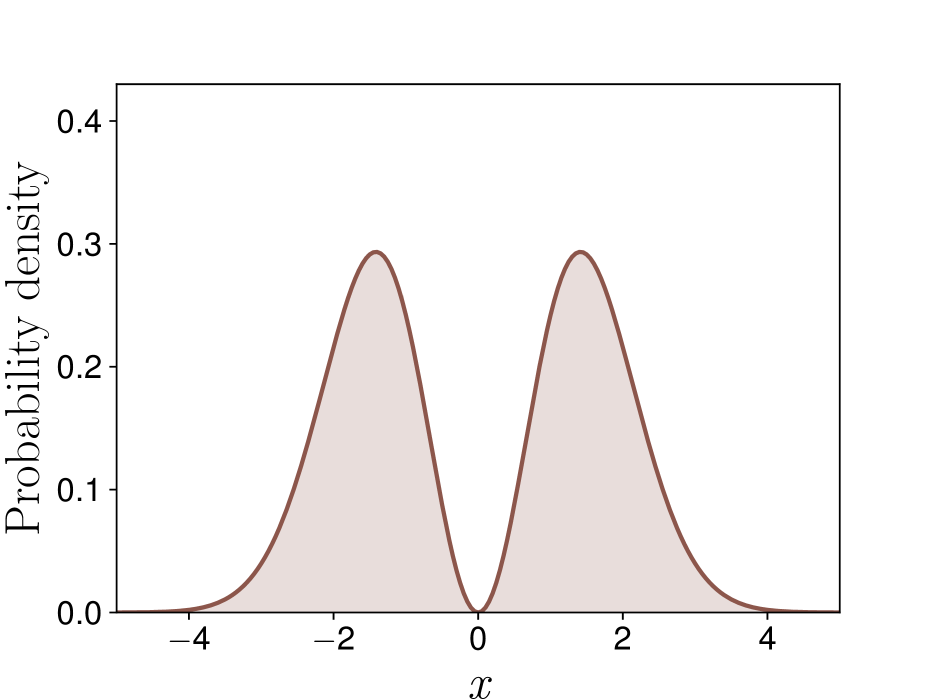
(b) Probability density

Figure 6: Slice integral sampling motivation and distribution for a Gaussian base distribution.

From Theorem 2 we saw that unlike the RP gradient case, the weighting $\psi$ for function values $\phi({\bm{x}})$ with ${\bm{x}}\sim p\left({\bm{x}};\theta\right)$ to obtain an unbiased estimator for the gradient $\frac{\textup{d}\hfill}{\textup{d}\theta\hfill}\mathbb{E}\left[\phi({\bm{x}})\right]$ is unique. The only option to reduce the variance by changing the weighting would then be to sample from a different distribution $q({\bm{x}})$ via importance sampling. Motivated by the resemblance of the “boxes” theory in Sec. 3 to the Riemann integral, we propose to sample horizontal slices of probability mass resembling the Lebesgue integral. Such an approach appears attractive, because if the location of the slice is moved by modifying the parameters of the distribution (e.g., by changing the mean), then the derivative of the expected value of the integral over the slice will depend only on the value at the edges of the slice (because the probability density in the middle would not change). To obtain the gradient estimator, it will only be necessary to compute the probability density $q_{L}({\bm{x}};\theta)$. We derive such a “slice integral” distribution corresponding to the Gaussian distribution. The method resembles the seminal work by Neal, (2003) on slice sampling in Markov chain Monte Carlo methods. We call our new distribution the L-distribution, and it is plotted in Fig. 6(b). In retrospect, it turned out that this distribution is optimal under the assumption that $\phi(x)$ is linear.

Derivation of the pdf of the L-distribution:

One way to sample whole slices of a probability distribution would be to sample a height $h$ between 0 and $p_{\mathrm{max}}$ proportionally to the probability mass at that height. The probability mass at a height $h$ is just given by $2|x-\mu|$ where $x$ is such that $p\left(x;\mu,\sigma\right)=h$, i.e., $2|x-\mu|$ is the distance between the edges of $p\left(x;\mu,\sigma\right)$. The probability mass corresponding to $x$ is then given by $2|x-\mu|\textup{d}h$. Performing a change of coordinates to the $x$-domain, and splitting the mass between the two edges of the slice, we get $|x-\mu|\textup{d}h=|x-\mu|\left|\frac{\textup{d}p\left(x;\mu,\sigma\right)\hfill}{\textup{d}x\hfill}\right|\textup{d}x$. This gives a closed-form normalized pdf for the L-distribution:

$$q_{L}(x;\mu,\sigma)=|x-\mu|\left|\frac{\textup{d}p\left(x;\mu,\sigma\right)\hfill}{\textup{d}x\hfill}\right| =|x-\mu|p\left(x;\mu,\sigma\right)\frac{|x-\mu|}{\sigma^{2}}$$ (78)

$$=\frac{|x-\mu|^{2}}{\sqrt{2\pi}~{}\sigma^{3}}\exp\left(\frac{-(x-\mu)^{2}}{2\sigma^{2}}\right).$$

One can recognize that Eq. (78) is actually just a Maxwell-Boltzmann distribution reflected about the origin with the probability mass split between the two sides.

Sampling from the L-distribution:

To sample from this distribution, it is necessary to sample points proportionally to the length of the slices. It suffices to sample uniformly in the area under the curve in the space augmented with the height dimension $h$, then selecting the slice on which the sampled point lies. This can be achieved with the three steps: 1) sample a point from the base distribution: $x_{s}\sim p\left(x;\mu,\sigma\right)$, 2) sample a height: $h\sim\textup{unif}\left(0,p\left(x_{s};\mu,\sigma\right)\right)$, 3) sample $x$ from one of the two edges of the slice $p^{-1}(h;\mu,\sigma)=\{x:p\left(x;\theta\right)=h\}$, where $p^{-1}(h)$ inverts the pdf, and computes the locations of $x$ that give a probability density $h$. For the L-distribution, this can be achieved by sampling $\epsilon_{x}\sim\mathcal{N}(0,1)$ and $\epsilon_{h}\sim\textup{unif}(0,1)$ and transforming these by the equation:

$$x=\mu\pm\sigma\sqrt{-2\log(\epsilon_{h})+\epsilon_{x}^{2}}~{}.$$ (79)

Now it is straightforward to obtain the LR gradient estimator:

$$\frac{\textup{d}\hfill}{\textup{d}\mu\hfill}\mathbb{E}_{x\sim p\left(x;\theta\right)}\left[\phi(x)\right]=\mathbb{E}_{x\sim q(x;\theta)}\left[\frac{\frac{\textup{d}p\hfill}{\textup{d}\mu\hfill}}{q(x;\theta)}\phi(x)\right] =\mathbb{E}_{x\sim q(x;\theta)}\left[\frac{1}{x-\mu}\phi(x)\right]$$ (80)

$$=\mathbb{E}\left[\frac{\textup{sgn}(x-\mu)}{\sigma\sqrt{-2\log(\epsilon_{h})+\epsilon_{x}^{2}}}\phi(x)\right].$$

References

- Abel, (1895) Abel, N. H. (1895). Untersuchungen über die Reihe: 1+(m/1) x+ m·(m-1)/(1· 2)· x2+ m·(m-1)·(m-2)/(1· 2· 3)· x3+… Number 71. W. Engelmann.
- Asadi et al., (2017) Asadi, K., Allen, C., Roderick, M., Mohamed, A.-r., Konidaris, G., and Littman, M. (2017). Mean actor critic. stat, 1050:1.
- Ciosek and Whiteson, (2018) Ciosek, K. and Whiteson, S. (2018). Expected policy gradients. In Thirty-Second AAAI Conference on Artificial Intelligence.
- Cong et al., (2019) Cong, Y., Zhao, M., Bai, K., and Carin, L. (2019). Go gradient for expectation-based objectives. arXiv preprint arXiv:1901.06020.
- Conti et al., (2018) Conti, E., Madhavan, V., Such, F. P., Lehman, J., Stanley, K., and Clune, J. (2018). Improving exploration in evolution strategies for deep reinforcement learning via a population of novelty-seeking agents. In Advances in Neural Information Processing Systems, pages 5027–5038.
- Farquhar et al., (2019) Farquhar, G., Whiteson, S., and Foerster, J. (2019). Loaded dice: Trading off bias and variance in any-order score function estimators for reinforcement learning. arXiv preprint arXiv:1909.10549.
- Figurnov et al., (2018) Figurnov, M., Mohamed, S., and Mnih, A. (2018). Implicit reparameterization gradients. In Advances in Neural Information Processing Systems, pages 441–452.
- Foerster et al., (2018) Foerster, J., Farquhar, G., Al-Shedivat, M., Rocktäschel, T., Xing, E., and Whiteson, S. (2018). Dice: The infinitely differentiable Monte Carlo estimator. In International Conference on Machine Learning, pages 1529–1538.
- Gal, (2016) Gal, Y. (2016). Uncertainty in deep learning. PhD thesis, PhD thesis, University of Cambridge.
- Geffner and Domke, (2018) Geffner, T. and Domke, J. (2018). Using large ensembles of control variates for variational inference. In Advances in Neural Information Processing Systems, pages 9960–9970.
- Glynn, (1990) Glynn, P. W. (1990). Likelihood ratio gradient estimation for stochastic systems. Communications of the ACM, 33(10):75–84.
- Grathwohl et al., (2017) Grathwohl, W., Choi, D., Wu, Y., Roeder, G., and Duvenaud, D. (2017). Backpropagation through the void: Optimizing control variates for black-box gradient estimation. arXiv preprint arXiv:1711.00123.
- (13) Greensmith, E., Bartlett, P. L., and Baxter, J. (2004a). Variance reduction techniques for gradient estimates in reinforcement learning. Journal of Machine Learning Research, 5(Nov):1471–1530.
- (14) Greensmith, E., Bartlett, P. L., and Baxter, J. (2004b). Variance reduction techniques for gradient estimates in reinforcement learning. Journal of Machine Learning Research, 5(Nov):1471–1530.
- Grinfeld, (2013) Grinfeld, P. (2013). Introduction to tensor analysis and the calculus of moving surfaces. Springer.
- Gu et al., (2015) Gu, S., Levine, S., Sutskever, I., and Mnih, A. (2015). MuProp: Unbiased backpropagation for stochastic neural networks. arXiv preprint arXiv:1511.05176.
- Gu et al., (2016) Gu, S., Lillicrap, T., Ghahramani, Z., Turner, R. E., and Levine, S. (2016). Q-prop: Sample-efficient policy gradient with an off-policy critic. arXiv preprint arXiv:1611.02247.
- Gu et al., (2017) Gu, S. S., Lillicrap, T., Turner, R. E., Ghahramani, Z., Schölkopf, B., and Levine, S. (2017). Interpolated policy gradient: Merging on-policy and off-policy gradient estimation for deep reinforcement learning. In Advances in Neural Information Processing Systems, pages 3846–3855.
- Ha and Schmidhuber, (2018) Ha, D. and Schmidhuber, J. (2018). Recurrent world models facilitate policy evolution. In Advances in Neural Information Processing Systems, pages 2450–2462.
- Hoffman et al., (2013) Hoffman, M. D., Blei, D. M., Wang, C., and Paisley, J. (2013). Stochastic variational inference. The Journal of Machine Learning Research, 14(1):1303–1347.
- Jang et al., (2016) Jang, E., Gu, S., and Poole, B. (2016). Categorical reparameterization with Gumbel-Softmax. arXiv preprint arXiv:1611.01144.
- Jankowiak and Karaletsos, (2019) Jankowiak, M. and Karaletsos, T. (2019). Pathwise derivatives for multivariate distributions. In The 22nd International Conference on Artificial Intelligence and Statistics, pages 333–342.
- Jankowiak and Obermeyer, (2018) Jankowiak, M. and Obermeyer, F. (2018). Pathwise derivatives beyond the reparameterization trick. In International Conference on Machine Learning, pages 2240–2249.
- Jiang and Li, (2016) Jiang, N. and Li, L. (2016). Doubly robust off-policy value evaluation for reinforcement learning. In International Conference on Machine Learning, pages 652–661.
- Jie and Abbeel, (2010) Jie, T. and Abbeel, P. (2010). On a connection between importance sampling and the likelihood ratio policy gradient. In Advances in Neural Information Processing Systems, pages 1000–1008.
- Kingma and Welling, (2013) Kingma, D. P. and Welling, M. (2013). Auto-encoding variational Bayes. arXiv preprint arXiv:1312.6114.
- L’Ecuyer, (1990) L’Ecuyer, P. (1990). A unified view of the IPA, SF, and LR gradient estimation techniques. Management Science, 36(11):1364–1383.
- L’Ecuyer, (1991) L’Ecuyer, P. (1991). An overview of derivative estimation. In 1991 Winter Simulation Conference Proceedings., pages 207–217. IEEE.
- Lee et al., (2018) Lee, W., Yu, H., and Yang, H. (2018). Reparameterization gradient for non-differentiable models. In Advances in Neural Information Processing Systems, pages 5553–5563.
- Liu et al., (2017) Liu, H., Feng, Y., Mao, Y., Zhou, D., Peng, J., and Liu, Q. (2017). Action-depedent control variates for policy optimization via stein’s identity. arXiv preprint arXiv:1710.11198.
- Maddison et al., (2016) Maddison, C. J., Mnih, A., and Teh, Y. W. (2016). The concrete distribution: A continuous relaxation of discrete random variables. arXiv preprint arXiv:1611.00712.
- Mania et al., (2018) Mania, H., Guy, A., and Recht, B. (2018). Simple random search of static linear policies is competitive for reinforcement learning. In Advances in Neural Information Processing Systems, pages 1800–1809.
- Mao et al., (2019) Mao, J., Foerster, J., Rocktäschel, T., Al-Shedivat, M., Farquhar, G., and Whiteson, S. (2019). A baseline for any order gradient estimation in stochastic computation graphs. In International Conference on Machine Learning, pages 4343–4351.
- Metz et al., (2019) Metz, L., Maheswaranathan, N., Nixon, J., Freeman, C. D., and Sohl-Dickstein, J. (2019). Understanding and correcting pathologies in the training of learned optimizers. In International Conference on Machine Learning.
- Mohamed et al., (2019) Mohamed, S., Rosca, M., Figurnov, M., and Mnih, A. (2019). Monte Carlo gradient estimation in machine learning. arXiv preprint arXiv:1906.10652.
- Munos et al., (2016) Munos, R., Stepleton, T., Harutyunyan, A., and Bellemare, M. (2016). Safe and efficient off-policy reinforcement learning. In Advances in Neural Information Processing Systems, pages 1054–1062.
- Neal, (2003) Neal, R. M. (2003). Slice sampling. The annals of statistics, 31(3):705–767.
- Nesterov and Spokoiny, (2017) Nesterov, Y. and Spokoiny, V. (2017). Random gradient-free minimization of convex functions. Foundations of Computational Mathematics, 17(2):527–566.
- Owen, (2013) Owen, A. B. (2013). Monte Carlo theory, methods and examples.
- Parmas, (2018) Parmas, P. (2018). Total stochastic gradient algorithms and applications in reinforcement learning. In Advances in Neural Information Processing Systems, pages 10204–10214.
- Parmas et al., (2018) Parmas, P., Rasmussen, C. E., Peters, J., and Doya, K. (2018). PIPPS: Flexible model-based policy search robust to the curse of chaos. In International Conference on Machine Learning, pages 4062–4071.
- Parmas and Sugiyama, (2019) Parmas, P. and Sugiyama, M. (2019). A unified view of likelihood ratio and reparameterization gradients and an optimal importance sampling scheme. arXiv preprint arXiv:1910.06419.
- Peters and Schaal, (2008) Peters, J. and Schaal, S. (2008). Reinforcement learning of motor skills with policy gradients. Neural networks, 21(4):682–697.
- Petersen and Pedersen, (2012) Petersen, K. B. and Pedersen, M. S. (2012). The matrix cookbook (version: November 15, 2012).
- Ranganath et al., (2016) Ranganath, R., Tran, D., and Blei, D. (2016). Hierarchical variational models. In International Conference on Machine Learning, pages 324–333.
- Rezende et al., (2014) Rezende, D. J., Mohamed, S., and Wierstra, D. (2014). Stochastic backpropagation and approximate inference in deep generative models. In International Conference on Machine Learning, pages 1278–1286.
- Riesz, (1907) Riesz, F. (1907). Sur une espèce de géométrie analytique des systèmes de fonctions sommables. Gauthier-Villars.
- (48) Ruiz, F., Titsias, M., and Blei, D. (2016a). Overdispersed black-box variational inference. In 32nd Conference on Uncertainty in Artificial Intelligence 2016, UAI 2016, pages 647–656.
- (49) Ruiz, F. J., Titsias, M. K., and Blei, D. (2016b). The generalized reparameterization gradient. In Advances in Neural Information Processing Systems, pages 460–468.
- Salimans et al., (2017) Salimans, T., Ho, J., Chen, X., Sidor, S., and Sutskever, I. (2017). Evolution strategies as a scalable alternative to reinforcement learning. arXiv preprint arXiv:1703.03864.
- (51) Schulman, J., Heess, N., Weber, T., and Abbeel, P. (2015a). Gradient estimation using stochastic computation graphs. In Advances in Neural Information Processing Systems, pages 3528–3536.
- (52) Schulman, J., Levine, S., Abbeel, P., Jordan, M., and Moritz, P. (2015b). Trust region policy optimization. In International Conference on Machine Learning, pages 1889–1897.
- Schulman et al., (2017) Schulman, J., Wolski, F., Dhariwal, P., Radford, A., and Klimov, O. (2017). Proximal policy optimization algorithms. arXiv preprint arXiv:1707.06347.
- Sutton and Barto, (1998) Sutton, R. S. and Barto, A. G. (1998). Reinforcement learning: An introduction, volume 1. MIT press Cambridge.
- Sutton et al., (2000) Sutton, R. S., McAllester, D. A., Singh, S. P., and Mansour, Y. (2000). Policy gradient methods for reinforcement learning with function approximation. In Advances in neural information processing systems, pages 1057–1063.
- Thomas and Brunskill, (2016) Thomas, P. and Brunskill, E. (2016). Data-efficient off-policy policy evaluation for reinforcement learning. In International Conference on Machine Learning, pages 2139–2148.
- Titsias and Lázaro-Gredilla, (2015) Titsias, M. K. and Lázaro-Gredilla, M. (2015). Local expectation gradients for black box variational inference. In Advances in neural information processing systems, pages 2638–2646.
- Tucker et al., (2018) Tucker, G., Bhupatiraju, S., Gu, S., Turner, R., Ghahramani, Z., and Levine, S. (2018). The mirage of action-dependent baselines in reinforcement learning. In International Conference on Machine Learning, pages 5022–5031.
- Tucker et al., (2017) Tucker, G., Mnih, A., Maddison, C. J., Lawson, J., and Sohl-Dickstein, J. (2017). REBAR: Low-variance, unbiased gradient estimates for discrete latent variable models. In Advances in Neural Information Processing Systems, pages 2627–2636.
- Walder et al., (2019) Walder, C. J., Nock, R., Ong, C. S., and Sugiyama, M. (2019). New tricks for estimating gradients of expectations. arXiv preprint arXiv:1901.11311.
- Weaver and Tao, (2001) Weaver, L. and Tao, N. (2001). The optimal reward baseline for gradient-based reinforcement learning. In Proceedings of the Seventeenth conference on Uncertainty in artificial intelligence, pages 538–545. Morgan Kaufmann Publishers Inc.
- Weber et al., (2019) Weber, T., Heess, N., Buesing, L., and Silver, D. (2019). Credit assignment techniques in stochastic computation graphs. In The 22nd International Conference on Artificial Intelligence and Statistics, pages 2650–2660.
- Wierstra et al., (2008) Wierstra, D., Schaul, T., Peters, J., and Schmidhuber, J. (2008). Natural evolution strategies. In 2008 IEEE Congress on Evolutionary Computation (IEEE World Congress on Computational Intelligence), pages 3381–3387. IEEE.
- Williams, (1992) Williams, R. J. (1992). Simple statistical gradient-following algorithms for connectionist reinforcement learning. Machine learning, 8(3-4):229–256.
- Wu, (2019) Wu, A. (2019). Generalized transformation-based gradient. arXiv preprint arXiv:1911.02681.
- Xu et al., (2019) Xu, M., Quiroz, M., Kohn, R., and Sisson, S. A. (2019). Variance reduction properties of the reparameterization trick. In International Conference on Artificial Intelligence and Statistics.

References

- Abel, (1895) Abel, N. H. (1895). Untersuchungen über die Reihe: 1+(m/1) x+ m·(m-1)/(1· 2)· x2+ m·(m-1)·(m-2)/(1· 2· 3)· x3+… Number 71. W. Engelmann.
- Asadi et al., (2017) Asadi, K., Allen, C., Roderick, M., Mohamed, A.-r., Konidaris, G., and Littman, M. (2017). Mean actor critic. stat, 1050:1.
- Ciosek and Whiteson, (2018) Ciosek, K. and Whiteson, S. (2018). Expected policy gradients. In Thirty-Second AAAI Conference on Artificial Intelligence.
- Cong et al., (2019) Cong, Y., Zhao, M., Bai, K., and Carin, L. (2019). Go gradient for expectation-based objectives. arXiv preprint arXiv:1901.06020.
- Conti et al., (2018) Conti, E., Madhavan, V., Such, F. P., Lehman, J., Stanley, K., and Clune, J. (2018). Improving exploration in evolution strategies for deep reinforcement learning via a population of novelty-seeking agents. In Advances in Neural Information Processing Systems, pages 5027–5038.
- Farquhar et al., (2019) Farquhar, G., Whiteson, S., and Foerster, J. (2019). Loaded dice: Trading off bias and variance in any-order score function estimators for reinforcement learning. arXiv preprint arXiv:1909.10549.
- Figurnov et al., (2018) Figurnov, M., Mohamed, S., and Mnih, A. (2018). Implicit reparameterization gradients. In Advances in Neural Information Processing Systems, pages 441–452.
- Foerster et al., (2018) Foerster, J., Farquhar, G., Al-Shedivat, M., Rocktäschel, T., Xing, E., and Whiteson, S. (2018). Dice: The infinitely differentiable Monte Carlo estimator. In International Conference on Machine Learning, pages 1529–1538.
- Gal, (2016) Gal, Y. (2016). Uncertainty in deep learning. PhD thesis, PhD thesis, University of Cambridge.
- Geffner and Domke, (2018) Geffner, T. and Domke, J. (2018). Using large ensembles of control variates for variational inference. In Advances in Neural Information Processing Systems, pages 9960–9970.
- Glynn, (1990) Glynn, P. W. (1990). Likelihood ratio gradient estimation for stochastic systems. Communications of the ACM, 33(10):75–84.
- Grathwohl et al., (2017) Grathwohl, W., Choi, D., Wu, Y., Roeder, G., and Duvenaud, D. (2017). Backpropagation through the void: Optimizing control variates for black-box gradient estimation. arXiv preprint arXiv:1711.00123.
- (13) Greensmith, E., Bartlett, P. L., and Baxter, J. (2004a). Variance reduction techniques for gradient estimates in reinforcement learning. Journal of Machine Learning Research, 5(Nov):1471–1530.
- (14) Greensmith, E., Bartlett, P. L., and Baxter, J. (2004b). Variance reduction techniques for gradient estimates in reinforcement learning. Journal of Machine Learning Research, 5(Nov):1471–1530.
- Grinfeld, (2013) Grinfeld, P. (2013). Introduction to tensor analysis and the calculus of moving surfaces. Springer.
- Gu et al., (2015) Gu, S., Levine, S., Sutskever, I., and Mnih, A. (2015). MuProp: Unbiased backpropagation for stochastic neural networks. arXiv preprint arXiv:1511.05176.
- Gu et al., (2016) Gu, S., Lillicrap, T., Ghahramani, Z., Turner, R. E., and Levine, S. (2016). Q-prop: Sample-efficient policy gradient with an off-policy critic. arXiv preprint arXiv:1611.02247.
- Gu et al., (2017) Gu, S. S., Lillicrap, T., Turner, R. E., Ghahramani, Z., Schölkopf, B., and Levine, S. (2017). Interpolated policy gradient: Merging on-policy and off-policy gradient estimation for deep reinforcement learning. In Advances in Neural Information Processing Systems, pages 3846–3855.
- Ha and Schmidhuber, (2018) Ha, D. and Schmidhuber, J. (2018). Recurrent world models facilitate policy evolution. In Advances in Neural Information Processing Systems, pages 2450–2462.
- Hoffman et al., (2013) Hoffman, M. D., Blei, D. M., Wang, C., and Paisley, J. (2013). Stochastic variational inference. The Journal of Machine Learning Research, 14(1):1303–1347.
- Jang et al., (2016) Jang, E., Gu, S., and Poole, B. (2016). Categorical reparameterization with Gumbel-Softmax. arXiv preprint arXiv:1611.01144.
- Jankowiak and Karaletsos, (2019) Jankowiak, M. and Karaletsos, T. (2019). Pathwise derivatives for multivariate distributions. In The 22nd International Conference on Artificial Intelligence and Statistics, pages 333–342.
- Jankowiak and Obermeyer, (2018) Jankowiak, M. and Obermeyer, F. (2018). Pathwise derivatives beyond the reparameterization trick. In International Conference on Machine Learning, pages 2240–2249.
- Jiang and Li, (2016) Jiang, N. and Li, L. (2016). Doubly robust off-policy value evaluation for reinforcement learning. In International Conference on Machine Learning, pages 652–661.
- Jie and Abbeel, (2010) Jie, T. and Abbeel, P. (2010). On a connection between importance sampling and the likelihood ratio policy gradient. In Advances in Neural Information Processing Systems, pages 1000–1008.
- Kingma and Welling, (2013) Kingma, D. P. and Welling, M. (2013). Auto-encoding variational Bayes. arXiv preprint arXiv:1312.6114.
- L’Ecuyer, (1990) L’Ecuyer, P. (1990). A unified view of the IPA, SF, and LR gradient estimation techniques. Management Science, 36(11):1364–1383.
- L’Ecuyer, (1991) L’Ecuyer, P. (1991). An overview of derivative estimation. In 1991 Winter Simulation Conference Proceedings., pages 207–217. IEEE.
- Lee et al., (2018) Lee, W., Yu, H., and Yang, H. (2018). Reparameterization gradient for non-differentiable models. In Advances in Neural Information Processing Systems, pages 5553–5563.
- Liu et al., (2017) Liu, H., Feng, Y., Mao, Y., Zhou, D., Peng, J., and Liu, Q. (2017). Action-depedent control variates for policy optimization via stein’s identity. arXiv preprint arXiv:1710.11198.
- Maddison et al., (2016) Maddison, C. J., Mnih, A., and Teh, Y. W. (2016). The concrete distribution: A continuous relaxation of discrete random variables. arXiv preprint arXiv:1611.00712.
- Mania et al., (2018) Mania, H., Guy, A., and Recht, B. (2018). Simple random search of static linear policies is competitive for reinforcement learning. In Advances in Neural Information Processing Systems, pages 1800–1809.
- Mao et al., (2019) Mao, J., Foerster, J., Rocktäschel, T., Al-Shedivat, M., Farquhar, G., and Whiteson, S. (2019). A baseline for any order gradient estimation in stochastic computation graphs. In International Conference on Machine Learning, pages 4343–4351.
- Metz et al., (2019) Metz, L., Maheswaranathan, N., Nixon, J., Freeman, C. D., and Sohl-Dickstein, J. (2019). Understanding and correcting pathologies in the training of learned optimizers. In International Conference on Machine Learning.
- Mohamed et al., (2019) Mohamed, S., Rosca, M., Figurnov, M., and Mnih, A. (2019). Monte Carlo gradient estimation in machine learning. arXiv preprint arXiv:1906.10652.
- Munos et al., (2016) Munos, R., Stepleton, T., Harutyunyan, A., and Bellemare, M. (2016). Safe and efficient off-policy reinforcement learning. In Advances in Neural Information Processing Systems, pages 1054–1062.
- Neal, (2003) Neal, R. M. (2003). Slice sampling. The annals of statistics, 31(3):705–767.
- Nesterov and Spokoiny, (2017) Nesterov, Y. and Spokoiny, V. (2017). Random gradient-free minimization of convex functions. Foundations of Computational Mathematics, 17(2):527–566.
- Owen, (2013) Owen, A. B. (2013). Monte Carlo theory, methods and examples.
- Parmas, (2018) Parmas, P. (2018). Total stochastic gradient algorithms and applications in reinforcement learning. In Advances in Neural Information Processing Systems, pages 10204–10214.
- Parmas et al., (2018) Parmas, P., Rasmussen, C. E., Peters, J., and Doya, K. (2018). PIPPS: Flexible model-based policy search robust to the curse of chaos. In International Conference on Machine Learning, pages 4062–4071.
- Parmas and Sugiyama, (2019) Parmas, P. and Sugiyama, M. (2019). A unified view of likelihood ratio and reparameterization gradients and an optimal importance sampling scheme. arXiv preprint arXiv:1910.06419.
- Peters and Schaal, (2008) Peters, J. and Schaal, S. (2008). Reinforcement learning of motor skills with policy gradients. Neural networks, 21(4):682–697.
- Petersen and Pedersen, (2012) Petersen, K. B. and Pedersen, M. S. (2012). The matrix cookbook (version: November 15, 2012).
- Ranganath et al., (2016) Ranganath, R., Tran, D., and Blei, D. (2016). Hierarchical variational models. In International Conference on Machine Learning, pages 324–333.
- Rezende et al., (2014) Rezende, D. J., Mohamed, S., and Wierstra, D. (2014). Stochastic backpropagation and approximate inference in deep generative models. In International Conference on Machine Learning, pages 1278–1286.
- Riesz, (1907) Riesz, F. (1907). Sur une espèce de géométrie analytique des systèmes de fonctions sommables. Gauthier-Villars.
- (48) Ruiz, F., Titsias, M., and Blei, D. (2016a). Overdispersed black-box variational inference. In 32nd Conference on Uncertainty in Artificial Intelligence 2016, UAI 2016, pages 647–656.
- (49) Ruiz, F. J., Titsias, M. K., and Blei, D. (2016b). The generalized reparameterization gradient. In Advances in Neural Information Processing Systems, pages 460–468.
- Salimans et al., (2017) Salimans, T., Ho, J., Chen, X., Sidor, S., and Sutskever, I. (2017). Evolution strategies as a scalable alternative to reinforcement learning. arXiv preprint arXiv:1703.03864.
- (51) Schulman, J., Heess, N., Weber, T., and Abbeel, P. (2015a). Gradient estimation using stochastic computation graphs. In Advances in Neural Information Processing Systems, pages 3528–3536.
- (52) Schulman, J., Levine, S., Abbeel, P., Jordan, M., and Moritz, P. (2015b). Trust region policy optimization. In International Conference on Machine Learning, pages 1889–1897.
- Schulman et al., (2017) Schulman, J., Wolski, F., Dhariwal, P., Radford, A., and Klimov, O. (2017). Proximal policy optimization algorithms. arXiv preprint arXiv:1707.06347.
- Sutton and Barto, (1998) Sutton, R. S. and Barto, A. G. (1998). Reinforcement learning: An introduction, volume 1. MIT press Cambridge.
- Sutton et al., (2000) Sutton, R. S., McAllester, D. A., Singh, S. P., and Mansour, Y. (2000). Policy gradient methods for reinforcement learning with function approximation. In Advances in neural information processing systems, pages 1057–1063.
- Thomas and Brunskill, (2016) Thomas, P. and Brunskill, E. (2016). Data-efficient off-policy policy evaluation for reinforcement learning. In International Conference on Machine Learning, pages 2139–2148.
- Titsias and Lázaro-Gredilla, (2015) Titsias, M. K. and Lázaro-Gredilla, M. (2015). Local expectation gradients for black box variational inference. In Advances in neural information processing systems, pages 2638–2646.
- Tucker et al., (2018) Tucker, G., Bhupatiraju, S., Gu, S., Turner, R., Ghahramani, Z., and Levine, S. (2018). The mirage of action-dependent baselines in reinforcement learning. In International Conference on Machine Learning, pages 5022–5031.
- Tucker et al., (2017) Tucker, G., Mnih, A., Maddison, C. J., Lawson, J., and Sohl-Dickstein, J. (2017). REBAR: Low-variance, unbiased gradient estimates for discrete latent variable models. In Advances in Neural Information Processing Systems, pages 2627–2636.
- Walder et al., (2019) Walder, C. J., Nock, R., Ong, C. S., and Sugiyama, M. (2019). New tricks for estimating gradients of expectations. arXiv preprint arXiv:1901.11311.
- Weaver and Tao, (2001) Weaver, L. and Tao, N. (2001). The optimal reward baseline for gradient-based reinforcement learning. In Proceedings of the Seventeenth conference on Uncertainty in artificial intelligence, pages 538–545. Morgan Kaufmann Publishers Inc.
- Weber et al., (2019) Weber, T., Heess, N., Buesing, L., and Silver, D. (2019). Credit assignment techniques in stochastic computation graphs. In The 22nd International Conference on Artificial Intelligence and Statistics, pages 2650–2660.
- Wierstra et al., (2008) Wierstra, D., Schaul, T., Peters, J., and Schmidhuber, J. (2008). Natural evolution strategies. In 2008 IEEE Congress on Evolutionary Computation (IEEE World Congress on Computational Intelligence), pages 3381–3387. IEEE.
- Williams, (1992) Williams, R. J. (1992). Simple statistical gradient-following algorithms for connectionist reinforcement learning. Machine learning, 8(3-4):229–256.
- Wu, (2019) Wu, A. (2019). Generalized transformation-based gradient. arXiv preprint arXiv:1911.02681.
- Xu et al., (2019) Xu, M., Quiroz, M., Kohn, R., and Sisson, S. A. (2019). Variance reduction properties of the reparameterization trick. In International Conference on Artificial Intelligence and Statistics.