Bounds on charged-lepton flavor violations via resonant scattering

Abstract

We explore the possibility of probing flavor violations in the charged-lepton sector by means of high-luminosity lepton-photon and electron-muon collisions, by inverting initial and final states in a variety of decay channels presently used to bound such violations. In particular, we analyse the resonant lepton, $\gamma\,\ell\to\ell^{\prime}$, and neutral-meson, $e^{\scriptscriptstyle-}\!\mu^{\scriptscriptstyle+}\to\phi,\eta,\pi^{0}\!$, scattering channels, whose cross sections are critically dependent on the colliding-beams energy spread, being particularly demanding in the case of leptonic processes. For these processes, we compute upper bounds to the cross-section corresponding to present limits on the inverse decay channel rates. In order to circumvent the beam energy spread limitations we extend the analysis to processes in which a photon accompanies the resonance in the final state, compensating the off-shellness effects by radiative return. These processes might be studied at future facilities with moderate energies, in case lepton-photon and electron-muon collisions with sufficiently high luminosity will be available.

I Introduction

Processes with violations of the generational leptonic number play a crucial role to test the standard model and to collect hints towards its possible extensions. While neutrino oscillations have been evidenced, lepton flavor violations for charged particles (CLFV hereafter) have not yet been observed. Some contribution to CLFV is expected in the standard model incorporating massive and mixing neutrinos, but at a level beyond the detectability for any foreseeable future Marciano:1977wx ; Petcov:1976ff ; BWLee1 ; BWLee2 ; Langacker:1988up . Extensions of the standard model such as supersymmetric models or grand unified theories instead provide ranges for CLFV rates which can be of phenomenological interest  IHLee1 ; IHLee2 ; Barbieri:1995tw ; ArkaniHamed:1995fs ; Kosmas:1993ch ; Raidal:2008jk . After earlier attempts to detect such effects in the muon decay channel $\mu\rightarrow e\gamma$ Brooks:1999pu , the currently more stringent test is provided by the MEG experiment, which finds at 90%C.L. a branching-ratio (BR) bound ${\rm BR}(\mu\to e\gamma)<4.2\times 10^{-13}\,$ TheMEG:2016wtm ; Adam:2013gfn . A factor 10 sensitivity improvement is expected after the MEG II upgrade Baldini:2018nnn . Further improved constraints will be provided by muon electron conversion $\mu N\to eN$ experiments Bernstein:2019fyh ; Diociaiuti:2020yvo ; Yucel:2021vir ; Adamov:2018vin and electron-ion colliders Cirigliano:2021img .

In this letter we discuss a complementary method to constrain possible CLFV, obtained by time reversal from a typical two-body CLFV decay channel. For example, in the $\mu\to e\gamma$ case, one can consider the inverse resonant production of a muon by the fusion of an electron and a photon of appropriate energy, in the $\gamma e\to\mu$ scattering. This process takes advantage from the possibility to control the beam intensities of electrons and photons. In principle, high intensity electron beams, as the one used in synchrotron radiation sources, and high intensity photon sources might provide a higher sensitivity, and allow, in the absence of detected events, for more stringent CLFV bounds. While we will see that, due to the extremely narrow linewidth of the process, the $\gamma e^{\scriptscriptstyle-}\to\mu^{\scriptscriptstyle-}$ case is not viable, we will discuss in detail more promising processes with broader resonances as the ones involving the $\tau$ lepton and pseudoscalar/vector mesons.

As a possible way to cope with the critical limitations connected to the finite beam-energy spread, we will then extend the above discussion by analyzing non-resonant channels derived by radiative return from the previous class of resonant processes.

The plan of the letter is as follows. In Section II, we discuss the production cross sections for resonant lepton ($\gamma\,\ell\to\ell^{\prime}$) and neutral-meson ($e^{\scriptscriptstyle-}\!\mu^{\scriptscriptstyle+}\to\phi,\eta,\pi^{0}\!$) scattering channels, including beam energy-spread effects on which the results are critically dependent. Cross-section upper bounds are computed on the basis of present experimental limits on the corresponding inverse decay channels. In Section III, we go beyond the leading-order resonant cross sections, and present analytical results for the corresponding radiative-return channels assuming a lepton-flavor violating Lagrangian in the effective field theory (EFT) approach. Finally, in Section IV, we present our conclusions.

II CLFV processes as resonant phenomena

The observation of CLFV events in resonant production may proceed under very strict kinematic conditions, as discussed in the following by recalling quite general considerations. Let consider a generic resonant process induced by the scattering of the $a$ and $b$ states $a+b\to R\to f$, where $R$ is a resonance, and $f$ its decay final state. The $R$ production in $a\,b$ collisions, in the reference frame where the $a$ and $b$ momenta are parallel but opposite, occurs when the following condition is fulfilled

$$E_{a}E_{b}\;(1+\beta_{a}\beta_{b})=\frac{1}{2}(m_{R}^{2}-m_{a}^{2}-m_{b}^{2})\,,$$ (1)

with $\beta_{a,b}=p_{a,b}/E_{a,b}$, where $E_{a,b}$ and $p_{a,b}$ are the energies and corresponding (modulus of) momenta respectively, that for $E_{a,b}\gg m_{a,b}$ can be approximated as $E_{a}E_{b}\simeq(m_{R}^{2}-m_{a}^{2}-m_{b}^{2})/4$.

In order for the $R$ resonance to go on-shell, one in general needs an excellent control on the energy spread of the colliding beams. The beam energy distribution can usually be described by a Gaussian function (see for instance Greco:2016izi )

$$G(E,\Delta E) = \frac{1}{\sqrt{2\pi}\Delta E}\exp\left[-\frac{(E-E_{0})^{2}}{2\Delta E^{2}}\right]\,,$$ (2)

where $E_{0}$ is the energy for which the beam intensity is maximum and $\Delta E$ the beam energy spread. Then, the cross section which takes into account the effect of the beam broadening is obtained as a convolution integral in the beam energy $E$ of the Breit-Wigner (BW) distribution of the resonance with the Gaussian distribution of the beams in Eq. (2).

Before including possible beams energy spread, the resonant cross section, for center-of-mass energies $E$ close to the resonance rest energy $m_{R}$, and in the non-relativistic limit, is given by

$$\sigma(E)=\frac{(2J+1)\,{\mbox{BR\,}}_{\!i}{\mbox{BR\,}}_{\!f}}{(2S_{a}+1)(2S_{b}+1)}\frac{4\pi}{p^{2}}\frac{\Gamma_{R}^{2}}{4(E-m_{R})^{2}+\Gamma_{R}^{2}}\,,$$ (3)

where $J$ is the total angular momentum of the resonance, $S_{a(b)}$ the spin of the initial $a(b)$ state, ${\mbox{BR\,}}_{\!i}$ and ${\mbox{BR\,}}_{\!f}$ are the branching ratios of the resonance decays into the initial ($R\to a\,b$) and final ($R\to f$) state, respectively, and $p$ is the $a,b$ momentum in the $a+b$ center-of-mass frame.

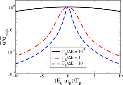
Figure 1: Reduction of the integrated cross-section due to the mismatching between the peak of the beams energy distribution and the resonance mass. The integrated cross-section normalized to the maximum of the cross-section $\bar{\sigma}_{\rm peak}$ is depicted versus the detuning factor $(E_{0}-m_{R})/\Gamma_{R}$, for three different values of the $\Gamma_{R}/\Delta E$ ratio, $10^{-1}$ (black, continuous), $1$(red, dot-dashed), and $10$ (blue, dotted).

Then, the integrated or averaged cross-section over the beam energy spread at $E\simeq m_{R}$ is given by

$$\bar{\sigma} \equiv \int_{-\infty}^{\infty}G(E,\Delta E)\sigma(E)dE\,.$$ (4)

In the case of a narrow resonance $\Gamma_{R}\ll m_{R}$ the last term in Eq. (3) can be well approximated by a Dirac delta-function distribution, namely

$$\frac{\Gamma_{R}^{2}}{4(E-m_{R})^{2}+\Gamma_{R}^{2}}\to\pi\frac{\Gamma_{R}}{2}\delta(E-m_{R})\,.$$ (5)

Then, in the narrow resonance approximation and for $\Gamma_{R}/\Delta E\ll 1$, by means of Eq. (5), the cross section in Eq. (4) simplifies to

$$\bar{\sigma} \simeq (2\pi)^{3/2}\frac{2J+1}{(2S_{a}+1)(2S_{b}+1)}\frac{{\mbox{BR\,}}_{\!i}{\mbox{BR\,}}_{\!f}}{2\,p_{R}^{2}}\,\frac{\Gamma_{R}}{\Delta E}\,,$$ (6)

with, neglecting initial particle masses, $p_{R}\simeq m_{R}/2$. Likewise, if the resonance is broad, the energy distribution of the beams can be approximated with a Dirac delta-function distribution.

In a generic intermediate case, that is when $\Gamma_{R}$ and $\Delta E$ are of the same order, one needs to numerically integrate the observable resonant cross section. In this case, we evaluate the averaged cross section in Eq.(4) by retaining the whole energy dependence in Eq. (3), except for the momentum $p$, which has been replaced by its value $p\sim m_{R}/2$ at the resonant energy $E=m_{R}$, a condition valid in the $\Gamma_{R}/m_{R}\ll 1$ limit. In Fig. 1 we show the integrated resonant cross-section $\bar{\sigma}$ in this general case, normalized to its peak value – that is relative to the case of an ideal tuning with a beam of negligible width – as a function of the energy detuning relative to the process linewidth, for different values of the ratio $\Gamma_{R}/\Delta E$. Notice that, by construction, the ratio plotted in Fig. 1 does not depend by the resonant mass $m_{R}$. As expected, the suppression is negligible if the resonance is narrower that the spread of the energy beam, as evidenced in the $\Gamma_{R}/\Delta E=10^{-1}$ case. However, in the opposite case of $\Gamma_{R}/\Delta E=10$, the reduction is considerable, for instance about two orders of magnitude for a detuning $|E_{0}-m_{R}|=5\Gamma_{R}$.

II.1 The $\gamma\ell\to\ell^{\prime}$ processes

We specialize here the considerations developed in the former section to the class of resonant FCNC processes in the charged lepton sector

$$\gamma\ell\to\ell^{\prime}\,,$$ (7)

for $\ell\neq\ell^{\prime}$, with $\ell=e,\mu$ and $\ell^{\prime}=\mu,\tau$. By taking into account the beam-energy broadening effect in Eq. (2), setting $E_{0}=m_{\ell^{\prime}}$ and $\Gamma=\Gamma_{\ell^{\prime}}$, with $m_{\ell^{\prime}}$ and $\Gamma_{\ell^{\prime}}$ the $\ell^{\prime}$ mass and width, respectively, and neglecting $m_{\ell}$, we obtain for the integrated resonant cross section

$$\bar{\sigma}(\gamma\ell\to\ell^{\prime}) \simeq \frac{(2\pi)^{3/2}}{m_{\ell^{\prime}}^{2}}\frac{\Gamma_{\ell^{\prime}}}{\Delta E}\;{\mbox{BR\,}}(\ell^{\prime}\to\ell\gamma)\,.$$ (8)

where in Eq. (6) we have replaced ${\mbox{BR\,}}_{\!i}\to{\mbox{BR\,}}(\ell^{\prime}\to\ell\gamma)$, and assumed ${\mbox{BR\,}}_{\!f}=1$.

We analyze first the most promising $\ell^{\prime}=\tau$ case, in particular the processes $\gamma e\to\tau$ and $\gamma\mu\to\tau$. By taking into account the $\tau$ total width $\Gamma_{\tau}\simeq 2.27\times 10^{-3}\,{\rm eV}$ and the present limits at 90% C.L. on the branching ratios for these processes, namely Aubert:2009ag

$${\rm BR}(\tau\to e\gamma)<3.3\times 10^{-8},\,{\rm BR}(\tau\to\mu\gamma)<4.4\times 10^{-8},$$ (9)

we get the following upper bounds for the corresponding resonant cross sections

$$\bar{\sigma}(\gamma e\to\tau) \;\stackrel{{\scriptstyle\textstyle<}}{{\sim}}\; 1.4\left(\frac{{\rm 100\,keV}}{\Delta E}\right)~{}{\rm ab}\,,$$ (10)

$$\bar{\sigma}(\gamma\mu\to\tau) \;\stackrel{{\scriptstyle\textstyle<}}{{\sim}}\; 1.9\left(\frac{{\rm 100\,keV}}{\Delta E}\right)~{}{\rm ab}\,.$$ (11)

Hence, assuming a beam energy spread $\Delta E\sim{\rm 100\,keV}$ in $\gamma e$ and $\gamma\mu$ collisions, measurements of the $\gamma\ell\to\tau$ cross sections of the order or smaller than $1\,{\rm ab}$ are required to achieve sensitivities on the branching ratios for the CLFV $\tau\to e\gamma$ and $\tau\to\mu\gamma$ decays which are comparable or stronger than the corresponding upper limits in Eq. (9).

It is also interesting to compare the latter cases with the more challenging resonant $\gamma e\to\mu$ production. With a muon lifetime of $\tau_{\mu}=2.2\times 10^{-6}$ s (corresponding to a total width $\Gamma_{\mu}=3.0\times 10^{-10}$ eV), muon production would require an unrealistic beam energy spread. Moreover, the extremely constraining MEG bound on the $\mu\rightarrow e\gamma$ decay (${\rm BR}(\mu\to e\gamma)\lower 4.30554pt\hbox{$\;\stackrel{{\scriptstyle\textstyle<}}{{\sim}}\;$}4.2\times 10^{-13}\,$ at 90% C.L. TheMEG:2016wtm ) implies an upper bound on the muon resonant cross section

$$\bar{\sigma}(\gamma e\to\mu) \;\stackrel{{\scriptstyle\textstyle<}}{{\sim}}\; 6.9\times 10^{-10}\left(\frac{{\rm 100\,keV}}{\Delta E}\right)~{}{\rm ab}\,.$$ (12)

which is beyond any realistic experimental performance by many orders of magnitude.

In preparation for the discussion presented in the next sections, it is useful to introduce an effective Lagrangian responsible for the CLFV $\ell^{\prime}\to\ell\gamma$ decay. This effective Lagrangian will be written in terms of the lowest (gauge-invariant) dimensional local operator given by the magnetic-dipole like interactions

$${\cal L}_{CLFV} = \sum_{\ell,\ell^{\prime}}\frac{1}{2\Lambda_{\ell^{\prime}\!\ell}}\bar{\psi}_{\ell}\sigma^{\alpha\beta}\psi_{\ell^{\prime}}~{}F_{\alpha\beta}+h.c.\,,$$ (13)

where $\Lambda_{\ell^{\prime}\!\ell}$ is the associated mass effective scale, $\psi_{\ell^{\prime}}$ and $\psi_{\ell}$ stand for the initial and final heavier lepton fields respectively, $F_{\alpha\beta}=\partial_{\alpha}A_{\beta}-\partial_{\beta}A_{\alpha}$ is the usual electromagnetic tensor operator, with $A_{\alpha}$ the photon field, and $\sigma^{\alpha\beta}\equiv i/2[\gamma^{\alpha},\gamma^{\beta}]$. In a potential UV completion for the new physics (NP) scenario, the effective interaction in Eq. (13) could arise for instance at one loop. In this case, the effective $\Lambda_{\ell^{\prime}\!\ell}$ scale is expected to be related to the mass and couplings of the NP scenario as $1/\Lambda_{\ell^{\prime}\!\ell}\sim g_{\ell^{\prime}\!\ell}^{2}/(16\pi^{2}M_{\rm NP})$, where $M_{\rm NP}$ stand for the smallest mass relevant to new physics running in the loop, and $g_{\ell^{\prime}\!\ell}\ll 1$ parametrizes the corresponding dimensionless CLFV coupling.

The decay width for $\ell^{\prime}\to\ell\gamma$ then becomes Gabrielli:2016cut

$$\Gamma(\ell^{\prime}\to\ell\gamma)=\frac{m_{\ell^{\prime}}^{3}}{8\pi\Lambda_{\ell^{\prime}\!\ell}^{2}}\left(1-r_{\ell}\right)^{3}\,,$$ (14)

with $r_{\ell}=m_{\ell}^{2}/m_{\ell^{\prime}}^{2}$. For instance, in the case of the CLFV $\mu\to e\gamma$ decay, by using the upper bound ${\mbox{BR\,}}(\mu\to e\gamma)<4.2\times 10^{-13}$, from Eq. (14) we obtain $\Lambda_{\mu e}\lower 4.30554pt\hbox{$\;\stackrel{{\scriptstyle\textstyle>}}{{\sim}}\;$}2\times 10^{10}~{}{\rm TeV}$ that, for $M_{\rm NP}\!\sim 10$ TeV, would imply for the relevant CLFV coupling $g_{\mu e}\!\lower 4.30554pt\hbox{$\;\stackrel{{\scriptstyle\textstyle<}}{{\sim}}\;$}3\times 10^{-4}$.

II.2 The $e^{\scriptscriptstyle-}\!\mu^{\scriptscriptstyle+}\to\phi,\eta,\pi^{0}$ processes

The severe bounds on the cross section for inverse CLFV processes like $e(\mu)\gamma\to\tau$ or $e\gamma\to\mu$ are due to both the extremely narrow width of the final state, and the strong experimental bound on the related branching ratios, especially in the $\mu\to e\gamma$ case. These two conditions are not satisfied for processes involving broader resonant states and less stringent experimental constraints on CLFV branching ratios (see Nussinov:2000nm for model-independent bounds based on unitarity).

In order to consider less constrained setups, we then extend our discussion to CLFV inverse processes involving neutral mesons, hence replacing $\gamma\ell$ initial states by opposite-charge leptons of different flavor. In particular, we will analyze the resonant CLFV production of a neutral meson $\rm M$, via the channel $e^{\pm}\mu^{\mp}\to\rm M\,$. Among many possibilities, we restrict the choice to the pseudoscalar mesons such as the neutral pion $\pi^{0}$ and the $\eta$, as well as the vector meson $\phi$. The considered mesons have widths much smaller than their mass, even in the broader $\phi$ case ($\Gamma_{\phi}/m_{\phi}\simeq 0.5\%$), and Eq. (6) still gives a proper description for the effective $e\mu\to\rm M$ cross sections.

The resonant $\rm M=\pi^{0}\!,\eta,\phi$ cross section averaged over the beam energy spread is then, analogously to Eq. (8) but retaining the exact muon mass ($m_{\mu}$) dependence,

$$\bar{\sigma}({e^{\scriptscriptstyle-}\!\mu^{\scriptscriptstyle+}\to\rm M})\simeq\frac{C_{\rm M}(2\pi)^{3/2}}{m_{\rm M}^{2}(1-r_{\mu})^{2}}\;\frac{\Gamma_{\rm M}}{\Delta E}\,\mbox{BR\,}(\rm M\to\mathnormal{e}^{-}\mu^{+}),\;\;\;\;\;$$ (15)

with $m_{\rm M}$ and $\Gamma_{\rm M}$ the $\rm M$ meson mass and width, respectively, while the coefficient $C_{\rm M}$ ($C_{\pi^{0}\!,\eta}=1/2$, and $C_{\phi}=3/2$) accounts for the $\rm M$ spin degeneracy, and $r_{\mu}=m_{\mu}^{2}/m^{2}_{\rm M}$.

By using the corresponding meson widths, $\Gamma_{\phi}\simeq 4.25~{}{\rm MeV}$, $\Gamma_{\eta}\simeq 1.31~{}{\rm keV}$, and $\Gamma_{\pi^{0}}\simeq 7.72~{}{\rm eV}$, and the present experimental upper limits on the CLFV branching ratios at 90% C.L.,

$${\rm BR}(\phi\to e\,\mu) \;\stackrel{{\scriptstyle\textstyle<}}{{\sim}}\; 2\times 10^{-6},~{}~{}~{}~{}~{}~{}\text{\cite[cite]{\@@bibref{Authors Phrase1YearPhrase2}{Achasov:2009en}{\@@citephrase{(}}{\@@citephrase{)}}}}$$

$${\rm BR}(\eta\to e\,\mu) \;\stackrel{{\scriptstyle\textstyle<}}{{\sim}}\; 6\times 10^{-6},~{}~{}~{}~{}~{}~{}\text{\cite[cite]{\@@bibref{Authors Phrase1YearPhrase2}{White:1995jc}{\@@citephrase{(}}{\@@citephrase{)}}}}$$

$${\rm BR}(\pi^{0}\!\to e\,\mu) \;\stackrel{{\scriptstyle\textstyle<}}{{\sim}}\; 3.6\times 10^{-10},~{}~{}~{}\text{\cite[cite]{\@@bibref{Authors Phrase1YearPhrase2}{Abouzaid:2007aa}{\@@citephrase{(}}{\@@citephrase{)}}}}$$ (16)

we obtain from Eq. (15) the following upper bounds on the cross sections

$$\bar{\sigma}(e^{\scriptscriptstyle-}\!\mu^{\scriptscriptstyle+}\to\phi) \;\stackrel{{\scriptstyle\textstyle<}}{{\sim}}\; 3.8\times 10^{2}\left(\frac{{\rm 100\,keV}}{\Delta E}\right){\rm nb}\,,$$ (17)

$$\bar{\sigma}(e^{\scriptscriptstyle-}\!\mu^{\scriptscriptstyle+}\to\eta) \;\stackrel{{\scriptstyle\textstyle<}}{{\sim}}\; 4.3\times 10^{2}\left(\frac{{\rm 100\,keV}}{\Delta E}\right){\rm pb}\,,$$ (18)

$$\bar{\sigma}(e^{\scriptscriptstyle-}\!\mu^{\scriptscriptstyle+}\to\pi^{0}) \;\stackrel{{\scriptstyle\textstyle<}}{{\sim}}\; 1.5\times 10^{-2}\!\left(\frac{{\rm 100\,keV}}{\Delta E}\right){\rm pb}\,.$$ (19)

In the latter equations, which include only one charge combination for the colliding particles, we use half of the BR’s experimental upper limits in Eqs. (16).

Electron-muon collisions in the energy range needed for the latter processes are indeed presently under consideration. The fixed target experiment MUonE plans to explore electron-muon scattering at $\sqrt{s}\simeq$ 400 MeV Banerjee:2020tdt . By running a similar experiment at lower $\sqrt{s}$, one in principle could cover the CLFV channel $e^{\scriptscriptstyle-}\!\mu^{\scriptscriptstyle+}\rightarrow\pi^{0}$, which has been investigated in the decay mode Krolak:1994aj ; Appel:2000tc , but has an expected $\pi^{0}\!\to e\,\mu$ partial width which is less than about $3\times 10^{-9}$ eV. With a modest boost in the energy with respect to MUonE, one could also reach the significantly broader $\eta$ resonance.

Notice that muon beams are expected to have a relative energy spread much smaller than their electron counterpart, due to the low impact of bremsstrahlung and synchrotron radiation, which is estimated to be at the Higgs-boson peak of the order of $\Delta E/E\simeq 10^{-5}$ Ankenbrandt:1999cta ; Raja:1998ip .

A different possibility might be provided by non fixed-target electron-muon setups. For instance, in order to go on the $\eta$ resonance, assuming an electron beam with $E_{e}$=50 MeV, one would need a muon beam with $E_{\mu}=$1.4 GeV. This combination could match the use of a high intensity electron beam from a van der Graaf accelerator (with order of $\mu$A currents) and a relatively high-energy muon beam with beam energy spread $\Delta E\simeq$ 15 keV, with a comparatively negligible electron beam energy spread.

In analogy to the purely leptonic channels, it is convenient to parametrize the effective CLFV coupling between the generic meson $\rm M$ (with $\rm M=\pi^{0},\eta$ for the case of scalar mesons, and $\rm M=\phi$ for the vector meson $\phi$) and the leptons. We assume the effective Lagrangian to be dominated by lowest dimensional operators of dimension 4. In particular, for the neutral scalar mesons $\rm M=\eta,\pi^{0}$, we parametrize it with operators of scalar Yukawa-type interaction

$${\cal L}^{S}_{\rm CLFV}=\left(Y^{L}_{\mu e}\bar{\psi}_{\mu}P_{L}\psi_{e}+Y^{R}_{\mu e}\bar{\psi}_{\mu}P_{R}\psi_{e}\right)\varphi_{M}+h.c.\,,~{}$$ (20)

where we assume the most general parity-violating couplings $Y^{L,R}_{\mu e}$ to the scalar meson $\rm M$ induced by some new physics, with the chiral projectors defined as $P_{L/R}=(1\mp\gamma_{5})/2$, and $\varphi$ stands generically for the scalar field associated to the scalar meson $\rm M$. On the other hand, for the vector meson $\phi$, we can parametrize the corresponding interaction as

$${\cal L}^{V}_{\rm CLFV}=\left(Y^{L}_{\mu e}\bar{\psi}_{\mu}\gamma^{\alpha}P_{L}\psi_{e}+Y^{R}_{\mu e}\bar{\psi}_{\mu}\gamma^{\alpha}P_{R}\psi_{e}\right)V_{\alpha}+h.c.\,,~{}$$ (21)

where $V_{\alpha}$ stands for the massive spin-1 field associated to the $\phi$ meson. To simplify the notations the same symbols for the couplings as in Eq.(20) have been adopted.

The effective couplings appearing in Eqs. (20,21) can originate at the fundamental level of quark and lepton interactions, via CLFV dimension 6 operators induced for instance by the exchange of some heavy new physics particle like

$${\cal L}_{\rm eff}\sim\frac{1}{\Lambda^{2}}[\bar{q}\Gamma_{i}q][\bar{\mu}\Gamma_{i}e]+h.c.\,,$$ (22)

where $q=u,d,s$ are the light quark fields, and $\Gamma_{i}$ generically indicate matrices of the Clifford basis (contraction over Lorentz indices is understood). For instance, in the case of a vectorial exchange, $\Gamma_{i}=\gamma_{\mu}$ or $\Gamma_{i}=\gamma_{\mu}\gamma_{5}$, one can easily relate the scale $\Lambda$ to the effective Yukawa coupling $Y^{L,R}_{\mu e}$ by making use of Lorentz invariance to compute the hadronic matrix element of the $\bar{q}\gamma_{\mu}\gamma_{5}q$ operator between the vacuum and the meson states. In particular, for the $\pi^{0}$ we have

$$Y^{L,R}_{\mu e}\sim\frac{f_{\pi}m_{\mu}}{\Lambda^{2}}\,,$$ (23)

with $f_{\pi}$ the pion decay constant, that for a new physics scale of the order of $\Lambda\simeq 1~{}{\rm TeV}$ yields $Y^{L,R}_{\mu e}\sim 10^{-8}$. Analogous results can be obtained for the $\eta$ and $\phi$ mesons, by applying the same considerations. Then, due to the short-distance nature of the quark-lepton interaction in Eq. (22), the validity of the effective meson interactions in Eqs. (20,21), is up to energies of the order of the scale $\Lambda$.

By using the effective Lagrangians in Eqs. (20,21), and by neglecting contributions proportional to $m_{e}$, we obtain, for the total width for the CLFV meson decay $\rm M\to\mathnormal{e}^{-}\!\mu^{+}$

$$\Gamma(\rm M\to\mathnormal{e}^{-}\!\mu^{+}) = \frac{S_{\rm M}|Y_{\mu e}|^{2}\;m_{\rm M}}{8\pi}\left(1-r_{\mu}\right)^{2}\,,$$ (24)

where $|Y_{\mu e}|^{2}\equiv\left(|Y^{L}_{\mu e}|^{2}+|Y^{R}_{\mu e}|^{2}\right)/2$, with spin factors $S_{\eta,\pi^{0}}=1$, $S_{\phi}=\left(2+r_{\mu}\right)/3$.

By using the bounds in Eq. (16) we can derive the upper limits at 90% C.L. on the corresponding CLFV couplings $Y_{\mu e}$ associated to the meson $\rm M$. In particular, we have

$$|Y_{\mu e}| < 4.0\times 10^{-4}\,,~{}~{}~{}\rm M=\phi$$

$$|Y_{\mu e}| < 1.4\times 10^{-5}\,,~{}~{}~{}\rm M=\eta$$

$$|Y_{\mu e}| < 4.2\times 10^{-8}\,,~{}~{}~{}\rm M=\pi^{0}\,.$$ (25)

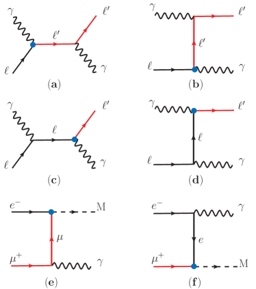
Figure 2: Tree-level Feynman diagrams for the radiative return processes $\gamma\ell\to\gamma\ell^{\prime}$ with $\ell\neq\ell^{\prime}$ (a-d), and $e^{\scriptscriptstyle-}\!\mu^{\scriptscriptstyle+}\to\rm M\gamma\,$ (e,f) with $\rm M=\phi,\eta,\pi^{0}$. The bubble vertex represents the proper effective CLFV interaction.

III Radiative return effects

It is clear from Eq. (8) that the $\Gamma_{\mu}/\Delta E$ ratio is a crucial factor affecting the resonant cross section, which can be particularly demanding in the case of a very narrow resonance, most notably in the leptonic cases considered above. This limitation can be circumvented by considering the radiative photon emission (giving rise, for instance, to the $\gamma e\rightarrow\gamma\mu$ process in the $\gamma e\rightarrow\mu$ case), an effect known as radiative return Yennie:1961ad ; Barger:1996jm . This has been mainly studied for the production of neutral resonant states (like $J/\Psi$, $Z^{0}$, Higgs boson) in $e^{\scriptscriptstyle+}\!e^{\scriptscriptstyle-}$ annihilation out of the resonant region, where it played a major role in the discovery of the $J/\Psi$. In these cases, its contribution can be reabsorbed into the initial-state-radiation (ISR) effects, which also include higher-order QED corrections and their exponentiation Yennie:1961ad ; Kuraev:1985hb ; Nicrosini:1986sm ; Jadach:2000ir .

In the next two subsections, we discuss possible advantages of the radiative-return channels for CLFV processes, distinguishing between the production of leptonic and mesonic final states.

III.1 The $\gamma\ell\to\gamma\ell^{\prime}$ processes

An extra photon emission in the $\gamma\ell\to\ell^{\prime}$ channel, where the resonance is a charged state, will involve both the initial and final states. Since the operator inducing the CLFV vertex for the $\ell\gamma\to\ell^{\prime}$ transition in Eq. (13) is a (dimension-5) magnetic-dipole operator, the $\gamma\ell\to\gamma\ell^{\prime}$ cross section will behave in the high energy limit in a dramatically different way with respect to the usual renormalizable interactions induced by dimension-4 operators. Indeed, we will see that it will tend to a constant in the asymptotic energy limit, against the usual $1/s$ cross-section behaviour of renormalizable interactions.

Here we provide an estimation of the upper bound of the CLFV $\gamma\ell\rightarrow\gamma\ell^{\prime}$ cross sections arising from radiative return effects, and compare them with the corresponding resonant processes cross sections discussed in section II.

Let us now consider the CLFV scattering process, induced by the Lagrangian in Eq. (13),

$$\gamma(q_{1})~{}e(p_{1})\to~{}\gamma(q_{2})~{}\mu(p_{2})\,,$$ (26)

where $p_{1,2}$ and $q_{1,2}$ are the relevant 4-momenta. The corresponding Feynman diagrams are shown in Fig. 2, panels (a-d). Generalizations to CLFV radiative transitions $\ell\to\ell^{\prime}$ involving other lepton flavors are straightforward. We obtain for the differential cross section for the process in Eq. (26)

$$\frac{d\sigma}{dt}(\gamma e\to\gamma\mu) \simeq \frac{\alpha}{2\Lambda_{\mu e}^{2}}\frac{F(s,t)}{(s-m_{\mu}^{2})^{2}+\Gamma_{\mu}^{2}m_{\mu}^{2}}\,,$$ (27)

where $\alpha$ is the fine structure constant evaluated at the $m_{\mu}$ scale, and $s=(p_{1}+q_{1})^{2}$, $t=(q_{1}-p_{2})^{2}$ are the Mandelstam variables. The function $F(s,t)$ is given by

$$F(s,t)=\frac{s+t-m_{\mu}^{2}}{s^{3}(t-m_{\mu}^{2})^{2}(t-m_{e}^{2})}\times$$

$$\Big{[}6s^{3}t^{3}-12m_{\mu}^{2}s^{2}t^{2}(s+t)+m_{\mu}^{4}st(7s^{2}+24st+7t^{2})-$$

$$m_{\mu}^{6}(s+t)(s^{2}+13st+t^{2})+12m_{\mu}^{8}st-m_{\mu}^{10}(s+t)\Big{)}\Big{]}\,,$$

where the electron mass $m_{e}$ is retained only in the denominator of the $t$-channel propagator, as needed to regularize the collinear divergencies. The exact expression for the function $F(s,t)$ with the full mass dependence is reported in Appendix A. For a soft final photon, in proximity of the kinematic threshold given by $s\sim m_{\mu}^{2}$, the resonant term in Eq. (27) is regularized by the muon width $\Gamma_{\mu}$.

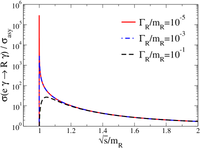
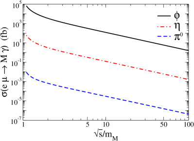
Figure 3: (Left) Cross section $\sigma(e\gamma\to R\gamma)$ versus $\sqrt{s}/m_{R}$, for the CLFV production of a fermion resonance $R$, normalized to the corresponding asymptotic cross section $\sigma_{\rm asy}(e\gamma\to R\gamma)$ at large $\sqrt{s}\gg m_{\rm R}$, for $m_{R}=m_{\mu}$, and $\Gamma_{R}/m_{R}=10^{-5}$ (red, continuous), $10^{-3}$ (blue, dot-dashed), $10^{-1}$ (black, dotted). (Right) Upper bounds on total cross sections for the $\rm M$ meson production $e^{\scriptscriptstyle-}\!\mu^{\scriptscriptstyle+}\to\rm M\gamma$, versus $\sqrt{s}/m_{\rm M}$, for $\rm M=\phi$ (black, continuous), $\rm M=\eta$ (red, dot-dashed), and $\rm M=\pi^{0}$ (blue, dotted). A cut $E_{\gamma}\lower 3.87498pt\hbox{$\;\stackrel{{\scriptstyle\textstyle>}}{{\sim}}\;$}m_{\rm M}/10$ is applied.

We first analyze this cross section in the asymptotic regime of center-of-mass energies $\sqrt{s}\gg m_{\mu}$, where $m_{\mu}$ (and hence $m_{e}$) can be neglected. By taking the massless limit in Eq. (27), we obtain

$$\frac{d\sigma_{\rm asy}}{dt}(\gamma e\to\gamma\mu)\simeq\frac{3\alpha}{\Lambda^{2}_{\mu e}}~{}\frac{s+t}{s^{2}}\,,$$ (28)

and by integrating Eq. (28) over the entire phase space ($-s\leq t\leq 0$), we get for the asymptotic total cross section

$$\sigma_{\rm asy}(\gamma e\to\gamma\mu)\simeq\frac{3\alpha}{2\Lambda_{\mu e}^{2}}\left(1+{\cal O}(m_{\mu}^{2}/s)\right).$$ (29)

The exact result, reported in Appendix A, allows to check that no powerlike singularities as from terms $\sim~{}\!\!\!1/t^{2}$, potentially modifying the expectations in Eq. (29) by contributions of the same order, arise in the muon and electron massless limit. The usual enhancement terms $\sim~{}\!\!\!\log{(s/m^{2}_{\ell})}$, arising from almost collinear, chirally suppressed, kinematic configurations, are all included in the last term of Eq. (29). Therefore, the leading contribution to the total cross section tends to a constant at high energies $\sqrt{s}\gg m_{\mu}$. This is simply due to dimensional reasons, being the effective operator in Eq. (13) of dimension 5. However, it should be kept in mind that the interaction in Eq. (13) is an effective low energy coupling, which is valid up to characteristic scattering energies of the order $\sqrt{s}\lower 4.30554pt\hbox{$\;\stackrel{{\scriptstyle\textstyle<}}{{\sim}}\;$}{\cal O}(\Lambda_{\mu e})$, above which a UV completion of the theory should be taken into account.

By using the $\mu\to e\gamma$ decay width in Eq. (14), we can rewrite the total cross section in Eq. (29) in terms of the branching ratio ${\rm BR}(\mu\to e\gamma)$ as

$$\sigma_{\rm asy}(\gamma e\to\gamma\mu)\simeq 12\pi\alpha\;\frac{\Gamma_{\mu}}{m^{3}_{\mu}}\;{\rm BR}(\mu\to e\gamma)\,,$$ (30)

which shows the insensitivity of the radiative return rate in the asymptotic regime to the beam energy spread. By using the existing experimental bound on $\mbox{BR\,}(\mu\to e\gamma)$, we get an upper limit on the asymptotic radiative cross section

$$\sigma_{\rm asy}(\gamma e\to\gamma\mu)\lower 4.30554pt\hbox{$\;\stackrel{{\scriptstyle\textstyle<}}{{\sim}}\;$}1.15\times 10^{-14}~{}{\rm ab}\,,$$ (31)

that is anyhow too tiny to give measurable effects.

Independently from the ${\mbox{BR\,}}(\mu\to e\gamma)$ bound, the CLFV resonant $e\gamma\to\mu$ cross section, as obtained from Eq. (8), is in general dominant with respect to the corresponding non-resonant $\gamma e\to\gamma\mu$ one. In the asymptotic regime of Eq. (29), their ratio is given by

$$\frac{\sigma_{\rm asy}(\gamma e\to\gamma\mu)}{\bar{\sigma}(e\gamma\to\mu)}\simeq\frac{6\alpha}{\sqrt{2\pi}}\frac{\Delta E}{m_{\mu}}\,,~{}$$ (32)

with the two cross sections becoming comparable for a beam energy spread $\Delta E\sim 57\,m_{\mu}$. Although neither cross sections are realistically measurable, in principle, for a typical beam energy spread of $\Delta E\sim 100\,{\rm keV}$, running on the $m_{\mu}$ pole would be more advantageous than looking at the radiative process with non-tuned collider facilities outside the resonant region.

Analogous results can be obtained for the more promising $\gamma e\to\gamma\tau$ and $\gamma\mu\to\gamma\tau$ processes, by properly replacing in Eq. (30) the muon width and mass, and the ${\rm BR}(\mu\to e\gamma)$ bound with the $\tau$ corresponding quantities. In particular, by using the upper limits in Eq. (9), we obtain

$$\sigma_{\rm asy}(\gamma e\to\gamma\tau) \;\stackrel{{\scriptstyle\textstyle<}}{{\sim}}\; 1.4\times 10^{-6}~{}{\rm ab}\,,$$

$$\sigma_{\rm asy}(\gamma\mu\to\gamma\tau) \;\stackrel{{\scriptstyle\textstyle<}}{{\sim}}\; 1.9\times 10^{-6}~{}{\rm ab}\,.$$ (33)

By extending Eq. (32) to the $\tau$ production, the radiative mode is confirmed to be sub-leading with respect to the resonant one, unless the energy spread becomes unrealistically large and of the order of at least $\Delta E\sim 100\,{\rm GeV}$.

On the other hand, in energy regions close to the resonance threshold, implying emissions of soft IR photons, the radiative $\gamma\ell\to\gamma\ell^{\prime}$ process can present a large enhancement inversely proportional to the resonance width. The exact total cross section, normalized to the asymptotic cross section, versus the center-of-mass energy $\sqrt{s}$ is shown in Fig. 3 (left plot) for a charged-lepton resonance $R$. For illustrative purposes we show three representative cases for the relative resonance width, $\Gamma_{R}/m_{R}=10^{-5},10^{-3},10^{-1}$, valid for $m_{R}=m_{\mu}$. The cross section peaks at more than $10^{5}$ its asymptotic value for the case of $\Gamma_{R}/m_{R}\simeq 10^{-5}$. Nevertheless, the potential gain in the radiative process is expected to be smeared out when convoluted with realistic beam energy spreads. The shapes of the curves in the left plot of Fig. 3 are almost independent on the mass $m_{R}$ in the resonant region, since this explicit dependence slightly affects the overall normalization alone.

For completeness, we provide an analytical approximated expression of the $\gamma e\to\gamma\mu$ total cross section valid for energies close to the threshold region $\sqrt{s}\simeq m_{\mu}$ (results can be generalized to different flavor radiative processes in a straightforward way). In particular, following the results in Appendix A, the total cross section near the resonant region can be written as

$$\sigma_{\rm thr}(\gamma e\to\gamma\mu) \simeq 8\pi\alpha\;C^{e\mu}_{F}\frac{\Gamma_{\mu}}{m_{\mu}}\;{\rm BR}(\mu\to e\gamma)\times$$ (34)

$$[\;\frac{s-m_{\mu}^{2}}{(s-m_{\mu}^{2})^{2}+\Gamma_{\mu}^{2}m_{\mu}^{2}}\;],~{}~{}$$

where $C^{e\mu}_{F}\simeq 8.7$ (see Appendix A) accounts for an average on the integrated angular distribution near the $\sqrt{s}$ peak value. The $s$-distribution in square brackets has a maximum $\sigma_{\rm peak}(\gamma e\to\gamma\mu)$ at $s=\bar{s}$ with $\bar{s}=m_{\mu}^{2}(1+\Gamma_{\mu}/m_{\mu})$, and vanishes at the threshold $s\to m_{\mu}^{2}$. The peak value for the cross section is

$$\sigma_{\rm peak}(\gamma e\to\gamma\mu)\simeq\frac{4\pi\alpha\,C^{e\mu}_{F}}{m_{\mu}^{2}}\;\mbox{BR\,}(\mu\to e\gamma)\,\lower 4.30554pt\hbox{$\;\stackrel{{\scriptstyle\textstyle<}}{{\sim}}\;$}\,12~{}{\rm fb}\,.$$

The corresponding peak values for $\tau$ production cross sections are

$$\sigma_{\rm peak}(\gamma e\to\gamma\tau)\lower 4.30554pt\hbox{$\;\stackrel{{\scriptstyle\textstyle<}}{{\sim}}\;$}\,5.3~{}{\rm pb}\,,$$

$$\sigma_{\rm peak}(\gamma\mu\to\gamma\tau)\lower 4.30554pt\hbox{$\;\stackrel{{\scriptstyle\textstyle<}}{{\sim}}\;$}\,1.8~{}{\rm pb}\,.$$ (35)

If we compare the above result with the BW cross section in Eq. (3), we find for the ratio of the radiative versus the non-radiative peak values

$$\frac{\sigma_{\rm peak}(\gamma e\to\gamma\mu)}{\sigma_{\rm peak}(\gamma e\to\mu)}\simeq\frac{\alpha}{2}C^{e\mu}_{F}\simeq 0.032\,,$$ (36)

where $\sigma_{\rm peak}$ is the corresponding BW distribution in Eq. (3) evaluated at the resonant energy $E=m_{R}$.

Then, for the averaged (according to the integral in Eq. (4) with $E_{0}\sim m_{\mu}$) radiative cross sections near the peak region, we obtain

$$\bar{\sigma}_{\rm thr}(\gamma e\to\gamma\mu)\simeq\frac{\alpha\,C^{e\mu}_{F}(2\pi)^{3/2}}{m_{\mu}^{2}}\frac{\Gamma_{\mu}}{\Delta E}\;\mbox{BR\,}(\mu\to e\gamma),$$ (37)

which is similar, apart from a numerical factor ($\sim\alpha$), to the result for the resonant BW cross section in Eq. (8). In deriving Eq. (37) the approximation of the relativistic version of the distribution in Eq. (5) for a narrow width has been used against the energy $E$ convolution integral in Eq. (4), namely $1/((s-m_{R}^{2})^{2}+\Gamma^{2}m_{R}^{2})\to\pi/(2\Gamma m_{R}^{2})\delta(E-m_{R})$, while the rest of the $s$ function appearing in Eq.(34) has been evaluated at its maximum value, that is for $s=\bar{s}$. Then the ratio of the convoluted (by beam energy spread effects) radiative cross section close to the threshold and the corresponding one for the BW production in Eq. (8) yields

$$\frac{\bar{\sigma}_{\rm thr}(\gamma e\to\gamma\mu)}{\bar{\sigma}(\gamma e\to\mu)}\simeq\alpha C^{e\mu}_{F},$$ (38)

which is approximatively twice the ratio of the unconvoluted peak cross sections in Eq. (36).

III.2 The $e^{-}\mu^{+}\to(\phi,\eta,\pi^{0})\,\gamma$ processes

We consider now the radiative return process applied to the resonant meson production $e^{\scriptscriptstyle-}\!\mu^{\scriptscriptstyle+}\to\rm M$

$$e^{-}(p_{1})\mu^{+}(p_{2})\to\rm M(q_{1})\gamma(q_{2})\,,$$ (39)

where $\rm M$ indicates a neutral meson, for the particular cases $\rm M=\phi,\eta,\pi^{0}$. As shown in the corresponding Feynman diagrams in Fig. 2 (e,f), the photon emission is uniquely due to initial state radiation.

CLFV Process	$E_{a}\times E_{b}({\mathrm{GeV^{2}}})$	$\Gamma_{\mathrm{tot}}({\mathrm{MeV}})$	BR${}_{\rm exp}^{\rm max}$	$\bar{\sigma}^{\rm max}_{(\Delta E=100~{}{\mathrm{keV}})}({\mathrm{fb}})$
$\gamma\mu\to\tau$	$7.9\times 10^{-1}$	$2.27\times 10^{-9}$	$4.4\times 10^{-8}$ Aubert:2009ag	$1.9\times 10^{-3}$
$\gamma e\to\tau$	$7.9\times 10^{-1}$	$2.27\times 10^{-9}$	$3.3\times 10^{-8}$ Aubert:2009ag	$1.4\times 10^{-3}$
$\gamma e\to\mu$	$2.8\times 10^{-3}$	$~{}3.00\times 10^{-16}$	$4.2\times 10^{-13}$ TheMEG:2016wtm	$~{}6.9\times 10^{-13}$
$e^{\scriptscriptstyle-}\!\mu^{\scriptscriptstyle+}\to\phi$	$2.6\times 10^{-1}$	$4.25$	$2.0\times 10^{-6}$ Achasov:2009en	$3.8\times 10^{8}$
$e^{\scriptscriptstyle-}\!\mu^{\scriptscriptstyle+}\to\eta$	$7.2\times 10^{-2}$	$1.31\times 10^{-3}$	$6.0\times 10^{-6}$ White:1995jc	$4.3\times 10^{5}$
$e^{\scriptscriptstyle-}\!\mu^{\scriptscriptstyle+}\to\pi^{0}$	$3.5\times 10^{-3}$	$7.72\times 10^{-6}$	$~{}3.6\times 10^{-10}$ ​Abouzaid:2007aa	$1.5\times 10^{1}$

Table 1: Summary of the inverse CFLV processes discussed in the text, with leptons and mesons in the final state. The columns report, for each process, the energy product from Eq. (1), the total resonance line-width, the current bound on the BR of the CLFV direct decay mode, and the corresponding bound on the integrated cross section for the inverse-decay scattering process, for $\sqrt{s}$ tuned at the resonance with a beam energy spread $\Delta E$ of $100~{}{\rm keV}$. All bounds on the CLFV branching ratios are at the $90\%$ confidence level. In the last row the product $E_{a}\times E_{b}$ corresponds to the frame in which one of the initial particles is at rest.

We keep the full $m_{\mu}$ dependence, and the $m_{e}$ dependence only in the denominator of the electron propagator in order to regularize the collinear divergencies. By using the effective Lagrangians in Eqs. (20,21), the differential cross section for the radiative return process in Eq. (39) becomes

$$\frac{d\sigma}{dt}(e^{\scriptscriptstyle-}\!\mu^{\scriptscriptstyle+}\to\rm M\gamma)\,=\,\frac{2\pi\alpha\,{\rm BR}(\rm M\to\mathnormal{e}^{-}\mu^{+})}{(1-\mathnormal{x}_{\mu})^{2}(1-\mathnormal{r}_{\mu})^{2}\mathnormal{S}_{M}}\;\frac{\Gamma_{\rm M}}{\it m_{\rm M}}{\mathnormal{F}}_{\rm M}(t)~{}~{}$$ (40)

where

$$F_{\eta,\pi^{0}}(t) = \frac{\mathnormal{x}_{\scriptscriptstyle{\rm M}}^{2}+1-2\mathnormal{x}_{\mu}}{(t-m_{\mu}^{2})(u-m_{e}^{2})}+\frac{2m_{\mu}^{2}(1-\mathnormal{x}_{\scriptscriptstyle{\rm M}})(\mathnormal{x}_{\scriptscriptstyle{\rm M}}-\mathnormal{x}_{\mu})}{(t-m_{\mu}^{2})^{2}(u-m_{e}^{2})}\,,$$

$$F_{\phi}(t) = \frac{2-5\mathnormal{x}_{\mu}+2\mathnormal{x}_{\scriptscriptstyle{\rm M}}(1+\mathnormal{x}_{\mu})+r_{\mu}(1-2\mathnormal{x}_{\mu})}{(t-m^{2}_{\mu})(u-m^{2}_{e})}$$ (41)

$$+ 2m_{\mu}^{2}\frac{\left(2\mathnormal{x}_{\scriptscriptstyle{\rm M}}-\mathnormal{x}_{\mu}(1+r_{\mu})\right)(1-\mathnormal{x}_{\scriptscriptstyle{\rm M}})}{(t-m_{\mu}^{2})^{2}(u-m_{e}^{2})}$$

$$+ \frac{3(1-\mathnormal{x}_{\scriptscriptstyle{\rm M}})-\mathnormal{x}_{\mu}}{s(u-m_{e}^{2})}+\frac{(t-m_{\mu}^{2})(3-5\mathnormal{x}_{\scriptscriptstyle{\rm M}})}{s^{2}(u-m_{e}^{2})(1-\mathnormal{x}_{\scriptscriptstyle{\rm M}})}\,,$$

with $x_{a}\equiv m^{2}_{a}/s$, $s=(p_{1}+p_{2})^{2}$, $t=(p_{1}-q_{1})^{2}$ and $u=(p_{1}-q_{2})^{2}$. By integrating over $t$, we get for the total cross section

$$\sigma(e^{\scriptscriptstyle-}\!\mu^{\scriptscriptstyle+}\to\rm M\gamma)\,=\,\frac{2\pi\alpha\,{\rm BR}(\rm M\to\mathnormal{e}^{-}\mu^{+})}{(1-\mathnormal{x}_{\mu})^{2}\mathnormal{s}(1-\mathnormal{r}_{\mu})^{2}\mathnormal{S}_{M}}\frac{\Gamma_{\rm M}}{\it m_{\rm M}}\mathnormal{\rho}_{M}(\mathnormal{x}_{\scriptscriptstyle{\rm M}},\mathnormal{x}_{\mu})\,,~{}~{}$$ (42)

where the ISR effect can be factorized by the function $\rho_{\rm M}(\mathnormal{x}_{\scriptscriptstyle{\rm M}},\mathnormal{x}_{\mu})$ given by

$$\!\!\!\!\rho_{\eta,\pi^{0}}(\mathnormal{x}_{\scriptscriptstyle{\rm M}},\mathnormal{x}_{\mu})=\frac{2}{(1-\mathnormal{x}_{\scriptscriptstyle{\rm M}})}\Big{[}(\mathnormal{x}_{\scriptscriptstyle{\rm M}}-\mathnormal{x}_{\mu})(\mathnormal{x}_{\mu}-1)+$$

$$(1+\mathnormal{x}_{\scriptscriptstyle{\rm M}}^{2}-2\mathnormal{x}_{\mu}-2\mathnormal{x}_{\scriptscriptstyle{\rm M}}\mathnormal{x}_{\mu}+2\mathnormal{x}_{\mu}^{2})L_{1}\Big{]}\,,$$

$$\!\!\!\!\rho_{\phi}(\mathnormal{x}_{\scriptscriptstyle{\rm M}},\mathnormal{x}_{\mu})=\frac{1}{(1-\mathnormal{x}_{\scriptscriptstyle{\rm M}})}\Big{[}2L_{1}\big{(}2-5\mathnormal{x}_{\mu}+2\mathnormal{x}_{\scriptscriptstyle{\rm M}}(1+\mathnormal{x}_{\mu})+$$

$$r_{\mu}(1-2\mathnormal{x}_{\mu})\big{)}-2(1-\mathnormal{x}_{\mu}(1-2L_{1})\big{)}(2\mathnormal{x}_{\scriptscriptstyle{\rm M}}-\mathnormal{x}_{\mu}(1+r_{\mu}))\Big{]}$$

$$+(3(\mathnormal{x}_{\scriptscriptstyle{\rm M}}-1)+\mathnormal{x}_{\mu})L_{2}+(5\mathnormal{x}_{\scriptscriptstyle{\rm M}}-3)(1-\mathnormal{x}_{\mu}-L_{2})\,,$$ (43)

where $L_{1}\equiv\log[(1-\mathnormal{x}_{\mu})/\sqrt{\mathnormal{x}_{\mu}x_{e}}]$, $L_{2}\equiv\log[(1-\mathnormal{x}_{\mu})/x_{e}]$.

The upper bounds (derived by the ${\rm BR}(\rm M\to\mu\mathnormal{e})$ upper limits in Eqs. (16)) for the $e^{\scriptscriptstyle-}\!\mu^{\scriptscriptstyle+}\to\rm M\gamma$ total cross sections versus $\sqrt{s}/m_{\rm M}$ are reported in the right plot of Fig. 3. The infrared divergence of the cross-section near resonance is tamed by requiring the detection of photons with energy $E_{\gamma}\lower 4.30554pt\hbox{$\;\stackrel{{\scriptstyle\textstyle>}}{{\sim}}\;$}m_{\rm M}/10$ Karliner:2015tga .

Although suppressed by the $\alpha$ factor with respect to the resonant case, these cross sections retain values within experimental observability with presumably realistic running times, relaxing the stringent demand for small energy spreads as in the resonant case.

It is also worth to point out that the effective Lagrangian approach, assuming pointlike and electrically neutral mesons, omits the emission of photons from the constituent quarks, the so-called structure-dependent emission, which is expected to contribute significantly at energies well above the threshold. Therefore our estimates at high energies should be considered as conservative, though in a regime which is anyway less favourable for the proposed experiments.

IV Summary and conclusions

The CLFV resonant productions considered in this analysis are summarized in Table I, where we show, for each process, a few relevant quantities that are crucial to the actual experimental implementation. The kinematical constraint is expressed in terms of the product of the beam energies to create the corresponding particle according to Eq. (1), providing some flexibility in the choice of the colliding beams. The processes involving neutral mesons might be feasible once high-luminosity muon beams will be available. The corresponding electron beam does not have to be at comparable high energy, therefore benefiting from the existence of less expensive high-intensity electron accelerators with energy in the (1-100) MeV range.

Purely leptonic resonating processes we have considered appear much more challenging. There is a certain complementarity in this regard, and processes with higher cross-sections are unfortunately harder to achieve kinematically. The $\gamma e\to\mu$ process would be quite feasible in terms of kinematics, for instance by using high-intensity electron beams as the one used in synchrotron radiation machines, with energy $E_{e}\simeq$ 2.8 GeV. This would imply the use of high-intensity photon beams centered around 1 MeV, i.e. in the $\gamma$-ray range. This is not a trivial requirement and, in the absence of high intensity $\gamma$-ray lasers, might be achieved only with high-intensity machines using inverse Compton scattering, but with unnaturally small energy spread. There are already $\gamma$-ray facilities which might be of some interest for this kind of experiments, such as ${\rm HI\gamma s}$ Weller and ELI-NP Filipescu , or proposed ones like the Gamma factory at CERN Budker . One could alternatively use high-intensity photon beams in the visible region, with $E_{\gamma}\simeq 1~{}\mathrm{eV}$, but only at the price of using electron beams with unrealistically high energy $E_{e}\simeq 2.8\times 10^{3}$ TeV. The $\gamma e\to\tau$and $\gamma\mu\to\tau$ cases have instead larger cross-sections, but the kinematics is less favourable, requiring high-energy muon beams with energy of order 1 TeV, and photon beams made of $\gamma$-rays in the 1 MeV range. Further analyses of the experimental feasibility of such collision setup will be required.

In conclusion, we have discussed the possibility of constraining lepton flavor violations in the charged sector using resonant and radiative-return processes, corresponding to the inverse of presently explored decay modes. In particular, we computed the upper bounds on the resonant lepton ($\gamma\,\ell\to\ell^{\prime}$) and neutral-meson ($e^{\scriptscriptstyle-}\!\mu^{\scriptscriptstyle+}\to\phi,\eta,\pi^{0}\!$) cross sections, and on the corresponding radiative processes. The characteristic of this approach is the possibility to control and boost the rates by proper engineering the beam luminosity setups. We have stressed the limitations due the the energy spread of the colliding beams, and discussed how to circumvent them by using the corresponding broadband radiative processes ($\gamma\,\ell\to\gamma\ell^{\prime}$ and $e^{\scriptscriptstyle-}\!\mu^{\scriptscriptstyle+}\to\gamma\,(\phi,\eta,\pi^{0})$), for which analytical cross sections have been computed by using an EFT approach.

The proposal is more effective for particles with large total width, and in this sense might generate competitive bounds, especially in the mesonic processes. For the purely leptonic processes, it seems that a strong effort for achieving beams with smaller energy spread is necessary, making this a further demand to the ongoing research and development on muon accelerators and high flux gamma sources Ankenbrandt:1999cta ; Gadjev:2017lvz ; Ping ; Raja:1998ip .

From the present discussion is clear that the actual sensitivity of the considered channels to possible CLFV effects will crucially depend on the luminosities and beams energy spread which can be actually reachable in the needed collision setup. On the other hand, here we did not focus on and discuss possible backgrounds of different nature, which in general will be as much crucial to set the actual potential of each channel and of the corresponding experimental signature. We leave a detailed discussion of this issue to future dedicated studies.

Appendix A Differential $\gamma e\to\gamma\mu$ cross section

Here we provide the exact expression for the differential cross section for the process $e(p_{1})\gamma(q_{1})\to\mu(p_{2})\gamma(q_{2})$ by retaining all the mass dependences. In particular we make explicit, in Eq.(27), the $F(s,t)$ function as

$$F(s,t) = \frac{u\sum_{k=0}^{10}m_{e}^{k}F^{(k)}(s,t)}{D(s,t)}\,,$$ (44)

with $D(s,t)=(s-m^{2}_{e})^{4}(t-m_{e}^{2})^{2}(t-m_{\mu}^{2})^{2}$, and $s,t$ are the Mandelstam variables as defined in Section III B, with $u=-s-t+m_{e}^{2}+m_{\mu}^{2}$. The functions $F^{(k)}(s,t)$ are given by

$$F^{(0)}(s,t) = -st\left(6s^{3}t^{3}-12m_{\mu}^{2}s^{2}t^{2}(s+t)+m_{\mu}^{4}st(7s^{2}+24st+7t^{2})-m_{\mu}^{6}(s+t)(s^{2}+13st+t^{2})+12m_{\mu}^{8}st-m_{\mu}^{10}(s+t)\right)\,,$$

$$F^{(1)}(s,t) = 2m_{\mu}s^{2}t^{2}(s-m_{\mu}^{2})(t-m_{\mu}^{2})(s+t-m_{\mu}^{2})\,,$$

$$F^{(2)}(s,t) = 12s^{3}t^{3}(s+t)-4m_{\mu}^{2}s^{2}t^{2}(3s+2t)(2s+3t)+m_{\mu}^{4}st(s+t)(13s^{2}+55st+13t^{2})$$

$$- m_{\mu}^{6}(s^{4}+38s^{3}t+50s^{2}t^{2}+38st^{3}+t^{4})+m_{\mu}^{8}(s+t)(2s^{2}+21st+2t^{2})-m_{\mu}^{10}(3s^{2}+2st+3t^{2})\,,$$

$$F^{(3)}(s,t) = 2m_{\mu}st(s-m_{\mu}^{2})(t-m_{\mu}^{2})(m_{\mu}^{4}-s^{2}-3st-t^{2})\,,$$

$$F^{(4)}(s,t) = -s^{2}t^{2}(7s^{2}+24st+7t^{2})+m_{\mu}^{2}st(s+t)(13s^{2}+55st+13t^{2})-2m_{\mu}^{4}(3s^{4}+24s^{3}t+76s^{2}t^{2}+24st^{3}+3t^{4})$$

$$+ 2m_{\mu}^{6}(s+t)(8s^{2}+33st+8t^{2})-7m_{\mu}^{8}(s^{2}+8st+t^{2})+5m_{\mu}^{10}(s+t)$$

$$F^{(5)}(s,t) = 2m_{\mu}(s-m_{\mu}^{2})(t-m_{\mu}^{2})(s+t)(2st+m_{\mu}^{2}(s+t)-m_{\mu}^{4})\,,$$

$$F^{(6)}(s,t) = st(s+t)(s^{2}+13st+t^{2})-m_{\mu}^{2}(s^{4}+38s^{3}t+50s^{2}t^{2}+38st^{3}+t^{4})+2m_{\mu}^{4}(s+t)(8s^{2}+33st+8t^{2})$$

$$- 6m_{\mu}^{6}(7s^{2}+8st+7t^{2})+19m_{\mu}^{8}(s+t)-4m_{\mu}^{10}\,,$$

$$F^{(7)}(s,t) = 2m_{\mu}(s-m_{\mu}^{2})(t-m_{\mu}^{2})(m_{\mu}^{4}-st-2m_{\mu}^{2}(s+t))\,,$$

$$F^{(8)}(s,t) = -12s^{2}t^{2}+m_{\mu}^{2}(s+t)(2s^{2}+21st+2t^{2})-7m_{\mu}^{4}(s^{2}+8st+t^{2})+19m_{\mu}^{6}(s+t)-6m_{\mu}^{8}\,,$$

$$F^{(9)}(s,t) = 2m_{\mu}^{3}(s-m_{\mu}^{2})(t-m_{\mu}^{2})\,,$$

$$F^{(10)}(s,t) = st(s+t)-m_{\mu}^{2}(3s^{2}+2st+3t^{2})+5m_{\mu}^{4}(s+t)-4m_{\mu}^{6}\,.$$

We now provide an approximate formula for the total cross section, valid for the kinematical regions $s\sim m_{\mu}^{2}$ close to the resonance muon threshold. For this aim, it is convenient to look at the angular distribution $\theta$, with $\theta$ the angle between the muon and electron momenta in the center-of-mass frame. In this case the variable $t$ can be expressed as

$$t=m_{e}^{2}-\frac{(s+m_{e}^{2})(s-m_{\mu}^{2})}{2s}\left(1-\beta_{e}\cos{\theta}\right)\,,$$ (45)

with $\beta_{e}=(s-m_{e}^{2})/(s+m_{e}^{2})$ the electron velocity. Then, the angular distribution for the cross section is given by

$$\frac{d\sigma}{d\cos{\theta}}(e\gamma\to\mu\gamma) = \frac{\alpha F(s,t)(1-r_{e})}{4\Lambda_{\mu e}^{2}}\times$$ (46)

$$\Big{[}\frac{s-m_{\mu}^{2}}{(s-m_{\mu}^{2})^{2}+\Gamma_{\mu}^{2}m_{\mu}^{2}}\Big{]}\,,$$

where $r_{e}=m^{2}_{e}/s$. Notice that the $s$ distribution inside the square brackets in Eq. (46) has a maximum for $s=\bar{s}$, where $\bar{s}\equiv m_{\mu}^{2}(1+\delta)$ with $\delta\sim\Gamma_{\mu}/m_{\mu}$, while the function $F(s,t)$ is almost flat in $s$ near regions close to $s\sim\bar{s}$. Therefore, in order to extract the dominant contribution to the total cross section relevant to the peak region, we approximate $F(s,t)$ with its expression evaluated at $s=\bar{s}$, thus by replacing $F(s,t)\to F(\bar{s},\bar{t})$, where $\bar{t}\equiv t|_{s=\bar{s}}$, and averaged it over $-1<\cos{\theta}<1$. In particular, by defining

$$\int_{-1}^{1}d\cos{\theta}~{}\frac{F(\bar{s},\bar{t})}{4}\equiv C^{e\mu}_{F}m_{\mu}^{2}\,,$$ (47)

the approximated total cross section near the threshold is

$$\sigma_{\rm thr}(\gamma e\to\gamma\mu) \simeq \frac{\alpha\;C^{e\mu}_{F}}{\Lambda_{\mu e}^{2}}\frac{\left(y_{s}-1\right)}{(y_{s}-1)^{2}+y^{2}_{\scriptscriptstyle{\Gamma_{\mu}}}}\,,$$ (48)

where $y_{a}\equiv a/m_{\mu}^{2}$. By numerical integrating Eq.(47) we obtain $C^{e\mu}_{F}\simeq 8.7$. The approximated formula in Eq. (48) fits with good accuracy the exact result, in particular, with an average of 20% accuracy in the range $m_{\mu}<\sqrt{s}<2m_{\mu}$ up to a few percent for $\sqrt{s}$ within 10% from the resonant mass.

For the analogous processes $\gamma e\to\gamma\tau$ and $\gamma\mu\to\gamma\tau$, the corresponding coefficients are $C^{e\tau}_{F}\simeq 14.3$   and  $C^{\mu\tau}_{F}\simeq 3.7$, respectively.

References

- (1) W. J. Marciano, A. I. Sanda, Exotic decays of the muon and heavy leptons in gauge theories, Phys. Lett. 67B (1977) 303-305.
- (2) S. T. Petcov, The processes , , in the Weinberg-Salam model with neutrino mixing, Sov. J. Nucl. Phys. 25 (1977) 340-344.
- (3) B. W. Lee, S. Pakvasa, R. E. Shrock, H. Sugawara, Muon and electron-number nonconservation in a gauge model, Phys. Rev. Lett. 38 (1977) 937-939.
- (4) B. W. Lee and R. E. Shrock, Natural suppression of symmetry violation in gauge theories: Muon- and electron-number nonconservation”, Phys. Rev. D16 (1977) 1444-1473.
- (5) P. Langacker, D. London, Lepton number violation and massless nonorthogonal neutrinos, Phys. Rev. D 38 (1988) 907-916.
- (6) I-H. Lee, Lepton number violation in softly broken supersymmetry, Phys. Lett. B 138 (1984) 121-127.
- (7) I-H. Lee, Lepton number violation in softly broken supersymmetry (II), Nucl. Phys. B 246 (1984) 120-142.
- (8) T. S. Kosmas, G. K. Leontaris, J. D. Vergados, Lepton flavor nonconservation, Prog. Part. Nucl. Phys. 33 (1994) 397-448, arXiv:hep-ph/9312217.
- (9) R. Barbieri, L. J. Hall, A. Strumia, Violations of lepton flavor and CP in supersymmetric unified theories, Nucl. Phys. B 445, 219-251 (1995) 219-251, arXiv:hep-ph/9501334.
- (10) N. Arkani-Hamed, H. C. Cheng, L. J. Hall, Flavor mixing signals for realistic supersymmetric unification, Phys. Rev. D 53 (1996) 413-436, arXiv:hep-ph/9508288.
- (11) M. Raidal, et al., Flavor physics of leptons and dipole moments, Eur. Phys. J C 57 (2008) 13-182, arXiv:hep-ph/0801.1826.
- (12) M. L. Brooks, et al. [MEGA], New limit for the family number nonconserving decay , Phys. Rev. Lett. 83 (1999) 1521-1524, arXiv:hep-ex/9905013.
- (13) A. M. Baldini, et al. [MEG], Search for the lepton flavour violating decay with the full dataset of the MEG experiment, Eur. Phys. J. C 76 (2016) 434, arXiv:1605.05081.
- (14) A. M. Baldini, et al. [MEG], Measurement of the radiative decay of polarized muons in the MEG experiment, Eur. Phys. J. C 76 (2016) 108, arXiv:1312.3217.
- (15) A. M. Baldini, et al. [MEG II], The design of the MEG II experiment, Eur. Phys. J. C 78 (2018) 380, arXiv:1801.04688.
- (16) R. H. Bernstein, The Mu2e Experiment, Front. in Phys. 7:1 (2019), arXiv:1901:11099.
- (17) E. Diociaiuti, conversion and the Mu2e experiment at Fermilab, PoS (EPS-HEP2019) (2020) 232.
- (18) M. Yucel, Muon to electron conversion search in the presence of Al nuclei at the Frmilab Mu2e experiment: Motivation, Design and Progress, PoS (ICHEP2020) (2021) 439.
- (19) R. Abramishvili, et al. [COMET], COMET Phase-I technical design report, Prog. Theor. Phys. 2020 (2020) 033C01, arXiv:1812.09018.
- (20) V. Cirigliano, K. Fuyuto, C. Lee, E. Mereghetti, B. Yan, Charged lepton flavor violation at the EIC, JHEP 03 (2021) 256, arXiv:2102.06176.
- (21) M. Greco, T. Han, Z. Liu, ISR effects for resonant Higgs production at future lepton colliders, Phys. Lett. B 763 (2016) 409-415, arXiv:1607.03210.
- (22) B. Aubert, et al. [BaBar], Searches for Lepton Flavor Violation in the Decays and , Phys. Rev. Lett. 104 (2010) 021802, arXiv:0908.2381
- (23) E. Gabrielli, B. Mele, M. Raidal, E. Venturini, FCNC decays of standard model fermions into a dark photon, Phys. Rev. D 94 (2016) 115013, arXiv:1607.05928.
- (24) S. Nussinov, R. D. Peccei, X. M. Zhang, On unitarity based relations between various lepton family violating processes, Phys. Rev. D 63, 016003 (2001) 016003, arXiv:hep-ph/0004153.
- (25) M. N. Achasov, et al., Search for lepton flavor violation process in the energy region and decay, Phys. Rev. D 81 (2010) 057102, arXiv:0911.1232.
- (26) D. B. White, et al., Search for the decays and , Phys. Rev. D 53 (1996) 6658-6661.
- (27) E. Abouzaid, et al. [KTeV], Search for lepton flavor violating decays of the neutral kaon, Phys. Rev. Lett. 100 (2008) 131803, arXiv:0711.3472.
- (28) P. Banerjee, et al., Theory for muon-electron scattering @ 10 ppm: A report of the MUonE theory initiative, Eur. Phys. J. C 80 (2020) 591, arXiv:2004.13663.
- (29) P. Krolak, et al., A Limit on the lepton family number violating process FNAL-799 experiment, Phys. Lett. B 320 (1994) 407-410.
- (30) R. Appel, et al., Search for lepton flavor violation in decays, Phys. Rev. Lett. 85 (2000) 2877-2880, arXiv:hep-ex/0006003.
- (31) C. M. Ankenbrandt, et al., Status of muon collider research and development and future plans, Phys. Rev. ST Accel. Beams 2 (1999) 081001, arXiv:physics/9901022.
- (32) R. Raja, A. Tollestrup, Calibrating the energy of a 50 GeV 50 GeV muon collider using spin precession, Phys. Rev. D 58 (1998) 013005, arXiv:hep-ex/9801004
- (33) D. R. Yennie, S. C. Frautschi, H. Suura, The infrared divergence phenomena and high-energy processes, Annals Phys. 13 (1961) 379-452.
- (34) V. D. Barger, M. S. Berger, J. F. Gunion, T. Han, Higgs Boson physics in the s channel at colliders, Phys. Rep. 286 (1997) 1-51, arXiv:hep-ph/9602415
- (35) E. A. Kuraev, V. S. Fadin, On radiative corrections to single photon annihilation at high-energy, Sov. J. Nucl. Phys. 41 (1985) 466-472.
- (36) O. Nicrosini, L. Trentadue, Soft photons and second order radiative corrections to , Phys. Lett. B 196 (1987) 551-556.
- (37) S. Jadach, B. F. L. Ward, Z. Was, Coherent exclusive exponentiation for precision Monte Carlo calculations, Phys. Rev. D 63 (2001) 113009, arXiv:hep-ph/0006359
- (38) M. Karliner, M. Low, J. L. Rosner, L. T. Wang, Radiative return capabilities of a high-energy, high-luminosity collider, Phys. Rev. D 92 (2015) 035010, arXiv:1503.07209.
- (39) H. R. Weller, et al., Research opportunities at the upgraded facility, Progr. Particle Nucl.Phys. 62 (2009) 257.
- (40) D. Filipescu, et al., Perspectives for photonuclear research at the Extreme Light Infrastructure - Nuclear Physics (ELI-NP) facility, Eur. Phys. J A 51 (2015) 185.
- (41) D. Budker, et al., Atomic physics studies at the Gamma Factory at CERN, Ann. Phys. 532 (2020) 2000204.
- (42) I. Gadjev, et al., An inverse free electron laser acceleration-driven Compton scattering X-ray source, Sci. Rep. 9 (2019) 532, arXiv:1711.00974.
- (43) Y. Ping, X. He, X., H. Zhang, B. Qiao, B., H. Cai, S. Chen, Gamma-ray source through inverse Compton scattering in a thermal hohlraum, Laser and Particle Beams, 31 (2013) 607-611.