Sparse Mixture Models inspired by ANOVA Decompositions

Abstract

Inspired by the analysis of variance (ANOVA) decomposition of functions we propose a Gaussian-Uniform mixture model on the high-dimensional torus which relies on the assumption that the function we wish to approximate can be well explained by limited variable interactions. We consider three approaches, namely wrapped Gaussians, diagonal wrapped Gaussians and products of von Mises distributions. The sparsity of the mixture model is ensured by the fact that its summands are products of Gaussian-like density functions acting on low dimensional spaces and uniform probability densities defined on the remaining directions. To learn such a sparse mixture model from given samples, we propose an objective function consisting of the negative log-likelihood function of the mixture model and a regularizer that penalizes the number of its summands. For minimizing this functional we combine the Expectation Maximization algorithm with a proximal step that takes the regularizer into account. To decide which summands of the mixture model are important, we apply a Kolmogorov-Smirnov test. Numerical examples demonstrate the performance of our approach.

1 Introduction

Most high-dimensional real-world systems are dominated by a small number of low-complexity interactions [55]. This is the background of extensive research to represent functions acting on high-dimensional data by functions defined on lower dimensional spaces. Approaches include active subspace methods [14, 15, 21] and random features [11, 26, 37, 48, 57].

This paper was inspired by the analysis of variance (ANOVA) decomposition of functions [10, 25, 28, 34, 38] which decomposes a function uniquely into the sum of functions depending on the different variable combinations. In practice it can often be assumed that the significant part of a functions can be explained by the simultaneous interactions of only a small number of variables, which is also in the spirit of [19]. The amazing result of Potts and Schmischke in [4, 47, 46] show that high-dimensional functions with a sparse ANOVA decomposition can be reconstructed using their approximation in the Fourier domain by rather few samples $t^{i}\in\mathbb{T}^{d}$ and $f(t^{i})\in\mathbb{R}$, $i=1,\ldots,N$. While the theory relies mainly on uniformly sampled points on the high-dimensional torus $\mathbb{T}^{d}$ or on $[0,1]^{d}$, also real-world data sets can be approximated in a way that beats state-of-the-art methods as the gradient boosting machine [23], random forest [23], sparse random features [26] and local learning regression neural networks [33].

In this paper, we assume that we are given high-dimensional samples $(x^{i})_{i}$ from a distribution with unknown probability density function $f$ rather than interpolation knots $(t^{i},f(t^{i}))_{i}$. Since e.g. attribute ranking can be used to remove unimportant variables immediately and to reduce the dimensionality of the problem, we concentrate on functions, where each variable has an influence, but not simultaneously with all other ones. Then, we are interested in mixture models with sparse components in the sense that they depend only on the data in smaller dimensions. We propose to learn such a mixture model by minimizing a penalized negative log-likelihhod function in connection with a Kolmogorov-Smirnov test to find the active variables in the summands of the mixture model. Once a mixture model is fitted, a natural way to identify the influence of attributes to the outcome is given by adjusting samples to the appropriate summands of the mixture.

Our model appears to be opposite to recently introduced mixture models which components rely on projections into sparse subspaces of the high-dimensional data space as mixtures of probabilistic PCAs (MPPCA) [54], high-dimensional data clustering (HDDC) [7], high-dimensional mixture models for unsupervised image denoising (HDMI) [30], and PCA-GMMs [27]. For more information, see Remark 2.4.

The paper is organized as follows: In Section 2, we first recall the sparse ANOVA decomposition on the $d$-dimensional torus. Then we introduce appropriate sparse mixture models having components which are products of a Gaussian-like density function on the $n$-dimensional torus ($n\ll d$) and a the uniform density on the $d-n$-dimensional torus. We propose three Gaussian-like settings, namely the wrapped normal distribution, the diagonal wrapped normal distribution, and products of von Mises distributions. Further, we discuss the ANOVA decomposition of the mixture models based on the notation of identifiable parameterized families of functions. Section 3 deals with the learning of the sparse mixture model. Based on an objective function consisting of the negative log-likelihood function penalized by a sparsity term for the number of coefficients, we propose to apply an Expectation Maximization (EM) algorithm in combination with a proximal step and a Kolmogorov-Smirnov test. Section 4 demonstrates the performance of our model by several examples. The code is available online. The Appendix A summarizes the EM algorithms for the tree Gaussian-like mixture models, and Appendix B briefly shows how the Kolmogorov-Smirnov test works.

2 ANOVA Decomposition and Mixture Models

Let $[d]\coloneqq\{1,...,d\}$ with the convention that $[0]=\emptyset$, and let $\mathcal{P}([d])$ be the power set of $[d]$. Further, for $u\subseteq[d]$, we write $u^{c}\coloneqq[d]\backslash u$ and $x_{u}\coloneqq(x_{i})_{i\in u}$. By $\mathbb{T}^{d}=\mathbb{R}^{d}/\mathbb{Z}^{d}=[0,1[^{d}$, we denote the $d$-dimensional torus and by $I_{d}$ the $d\times d$ identity matrix.

We are interested in the additive decomposition of integrable functions $f\mathrel{\mathop{\ordinarycolon}}\mathbb{T}^{d}\rightarrow\mathbb{R}$ into lower dimensional components

$$f(x)=\sum_{u\subseteq[d]}f_{u}(x_{u}),\quad f_{u}\colon\mathbb{T}^{|u|}\to\mathbb{R}.$$ (1)

In general, such decomposition is not unique. We rely on two special decompositions, namely the ANOVA decomposition which was the motivation of this work and sparse mixture models. In the following we introduce both concepts and explain their relation.

ANOVA decomposition

For any integrable function $f\mathrel{\mathop{\ordinarycolon}}\mathbb{T}^{d}\rightarrow\mathbb{R}$, there exists a unique decomposition of the form (1), the so-called analysis of variance (ANOVA) decomposition determined by

$$f_{u}\coloneqq(P_{u}f)-\sum_{v\varsubsetneq u}f_{v}=\sum_{v\subseteq u}(-1)^{|u|-|v|}P_{v}f,$$ (2)

where

$$(P_{u}f)(x)\coloneqq\int_{\mathbb{T}^{d-|u|}}f(x)\,dx_{u^{c}}.$$ (3)

The following proposition recalls that the ANOVA decomposition of a function which is the sum of lower dimensional functions can only contain summands acting on the same subspaces.

Proposition 2.1.

Let $W\subseteq\mathcal{P}([d])$. Then, a function $f$ of the form

$$f(x)=\sum_{w\in W}g_{w}(x_{w})$$ (4)

has an ANOVA decomposition of the form

$$f=\sum_{u\in\bar{W}}f_{u},$$

where $\bar{W}$ denotes the set $\{u\subseteq w\mathrel{\mathop{\ordinarycolon}}w\in W\}$.

Proof.

Let $T_{u}$ denote the linear operator which maps a function $f$ to its ANOVA component $f_{u}$. Then we have for the function in (4) that

$$f_{u}=T_{u}f=\sum_{w\in W}T_{u}g_{w}.$$

and it remains to show that for $w$ not containing $u$ it holds $T_{u}g_{w}=0$. Let $u$ be not contained in $w$. Using (2) and the facts that $g_{w}=P_{w}g_{w}$ and $P_{v}P_{u}=P_{v\cap u}$, we obtain

$$T_{u}g_{w} =\sum_{v\subseteq u}(-1)^{|u|-|v|}P_{v}g_{w}=\sum_{v\subseteq u}(-1)^{|u|-|v|}P_{v}P_{w}g_{w}=\sum_{v\subseteq u}(-1)^{|u|-|v|}P_{v\cap w}g_{w}.$$ (5)

If $v\cap w=\emptyset$, the assertion follows since $\sum_{v\subseteq u}(-1)^{|u|-|v|}=0$. Otherwise, we get with $n\coloneqq|u\setminus w|>0$ that

$$T_{u}g_{w} =\sum_{v_{1}\subseteq u\cap w}\sum_{v_{2}\subseteq u\setminus w}(-1)^{|u|-(|v_{1}|+|v_{2}|)}P_{v_{1}}g_{w}$$ (6)

$$=\sum_{v_{1}\subseteq u\cap w}(-1)^{|u|-|v_{1}|}P_{v_{1}}g_{w}\sum_{v_{2}\subseteq u\setminus w}(-1)^{|v_{2}|}$$ (7)

$$=\sum_{v_{1}\subseteq u\cap w}(-1)^{|u|-|v_{1}|}P_{v_{1}}g_{w}\sum_{j=0}^{n}\binom{n}{j}(-1)^{j}=0,$$ (8)

which gives the assertion. ∎

In real-world applications, it often appears that the decomposition (1) does not contain all subsets of $[d]$, but just a smaller amount of subsets $U\subset\mathcal{P}([d])$ which have cardinality not larger than some $n\ll d$ or that $f$ can be at least well approximated by a sparse ANOVA decomposition

$$\sum_{u\subseteq U}f_{u}(x_{u}).$$ (9)

Several authors examined the reconstruction of functions having such a sparse ANOVA approximation from values $\left(t^{i},f(t^{i})\right)$, $i=1,\ldots,N$ of $f$. The setting in this paper is different.

Remark 2.2 (Setting of this paper).

We deal with non-negative functions $f\colon\mathbb{T}^{d}\rightarrow\mathbb{R}$ on the $d$-dimensional torus $\mathbb{T}^{d}$ fulfilling $\|f\|_{L_{1}(\mathbb{T}^{d})}=1$ and consider them as probability density functions of a certain random variable $X\colon\Omega\rightarrow\mathbb{T}^{d}$. Instead of sampled function values, we assume that we are given samples $x^{i}$, $i=1,\ldots,N$ of the distribution with density $f$, i.e. realizations of the random variable $X$. This means that in contrast to the $t^{i}$, the samples $x^{i}$ inherit the properties of $f$. If the $t^{i}$, $i=1,\ldots,N$ are uniformly sampled, then clearly $f(t^{i})$ times $t^{i}$ may serve as samples, i.e., the $t^{i}$ must be weighted with the values $f(t^{i})$.

Sparse Mixture Models

In this paper, we aim to find an approximation of $f\in L_{1}(\mathbb{T}^{d})$ by a mixture model from samples of the corresponding distribution. For an introduction to mixture models we refer to [43]. To this end, let $\Delta_{K}\coloneqq\{\alpha\in\mathbb{R}^{K}_{\geq 0}\mathrel{\mathop{\ordinarycolon}}\alpha^{\mathrm{T}}1_{K}=1\}$ with the vector $1_{K}$ consisting of $K$ entries 1, be the probability simplex, and $\mathrm{SPD}(d)$ the cone of symmetric, positive definite matrices. Assume that $f$ can be approximated by mixture models of the form

$$p(x|\alpha,\vartheta)=\sum_{k=1}^{K}\alpha_{k}p_{u_{k}}(x_{u_{k}}|\vartheta_{k}),$$ (10)

where $u_{k}\in U\subset\mathcal{P}([d])$, $\alpha=(\alpha_{k})_{k=1}^{K}\in\Delta_{K}$, $\vartheta=(\vartheta_{k})_{k=1}^{K}$ and $p_{u_{k}}$ is a probability density functions on $\mathbb{T}^{n}$, $n=|u_{k}|$. Note that the index sets $u_{k}$ are in general not pairwise different, i.e. $u_{k}=u_{l}$ can appear for $k\not=l$. If $U$ contains only sets of small cardinality, we call (10) a sparse mixture model. Indeed, the density $p_{u}$ determines the distribution of a $\mathbb{T}^{d}$-valued random variable $X=(X_{u},X_{u^{c}})$ characterized by

$$(X_{u},X_{u^{c}})\sim p_{u}(\cdot|\vartheta)\times\mathcal{U}_{\mathbb{T}^{d-|u|}}.$$

This class of distributions includes for $u=\emptyset$ the uniform distribution on $\mathbb{T}^{d}$.

In this paper, we need the (absolutely continuous) normal or Gaussian distribution on $\mathbb{R}^{n}$ having the density function

$$\mathcal{N}(x|\mu,\Sigma)=(2\pi)^{-\frac{n}{2}}\mathinner{\!\left\lvert\Sigma\right\rvert}^{-\frac{1}{2}}\,\exp\left(-\frac{1}{2}(x-\mu)^{\mathrm{T}}\Sigma^{-1}(x-\mu)\right)$$ (11)

with mean $\mu\in\mathbb{R}^{n}$ and $\Sigma\in\mathrm{SPD}(n)$. This distribution has many characterizing properties which unfortunately cannot be transferred to a ,,normal distribution” on manifolds, see, e.g. [36]. In this paper, we restrict our attention to the normal-like distributions $p_{u_{k}}$ on the $n=|u_{k}|$ dimensional $\mathbb{T}^{n}$ listed in the following example.

Example 2.3.

We focus on mixture models on $\mathbb{T}^{d}$ with low dimensional components from one of the following distributions on $\mathbb{T}^{n}$, $n\ll d$:

• the wrapped normal distribution

  $$p_{G}(x|\mu,\Sigma)=\sum_{l\in\mathbb{Z}^{n}}\mathcal{N}(x+l|\mu,\Sigma)=\mathcal{N}_{w}(x|\mu,\Sigma),$$

  where $\mu\in\mathbb{T}^{n}$, $\Sigma\in\mathrm{SPD}(n)$. Note that $\mathcal{N}_{w}(\mu,\Sigma)$ is characterized by the distribution of $X-\lfloor X\rfloor$, where $X\sim\mathcal{N}(\mu,\Sigma)$. This formula allows us, to draw easily samples from $\mathcal{N}_{w}(\mu,\Sigma)$.

• the diagonal wrapped normal distribution

  $$p_{dG}(x|\mu,\sigma^{2})=p_{G}(x|\mu,\mathrm{diag}(\sigma^{2}))=\sum_{l\in\mathbb{Z}^{n}}\prod_{j=1}^{n}\mathcal{N}(x_{j}+l_{j}|\mu_{j},\sigma_{j}^{2})=\prod_{j=1}^{n}\mathcal{N}_{w}(x_{j}|\mu_{j},\sigma_{j}^{2}),$$

  where ($\mathcal{N}_{w}$) $\mathcal{N}$ is the univariate (wrapped) Gaussian density function and $\sigma^{2}\in\mathbb{R}^{n}_{>0}$.

• the von Mises distribution on $\mathbb{T}^{n}$ with parameters $\mu\in\mathbb{\mathbb{T}}^{n}$ and $\kappa\in\mathbb{R}^{n}_{>0}$ is the restriction of the probability density function of an isotropic normal distribution to the unit circle and has the probability density function

  $$p_{M}(x|\mu,\kappa)=\prod_{j=1}^{n}\tfrac{1}{I_{0}(\kappa_{j})}\exp\left(\kappa_{j}\cos\left(2\pi(x_{j}-\mu_{j})\right)\right),$$ (12)

  where $I_{0}$ is the modified Bessel function of first kind of order $0$. $\Box$

The wrapped normal distribution inherits by definition several properties of the normal distribution in $\mathbb{R}^{n}$. For example, we obtain directly for independent $X\sim\mathcal{N}_{w}(\mu,\Sigma)$, $Y\sim\mathcal{N}_{w}(\mu^{\prime},\Sigma^{\prime})$ that $X+Y\sim\mathcal{N}_{w}(\mu+\mu^{\prime},\Sigma+\Sigma^{\prime})$. Similarly, we get that any marginal of $X$ is again a wrapped normal distribution. Other properties of the normal distribution are not transferred to the wrapped case. For example, it holds on a circle that the von Mises distribution maximizes the entropy and not the wrapped normal distribution, see [31]. Indeed the von Mises distribution with parameters $(\mu,\kappa)$ is very similar to the one-dimensional wrapped normal distribution with parameters $(\mu,\sigma^{2})$, where the parameters are related via $\frac{I_{1}(\kappa)}{I_{0}(\kappa)}=\exp(-\tfrac{(2\pi)^{2}\sigma^{2}}{2})$, see [32]. Thus, the von Mises distribution is often used instead of the wrapped normal distributions with the benefit of a reduced complexity for evaluating the density function and estimating the parameters, see e.g. [8, 20, 35]. Unfortunately, there is no multivariate counterpart for this approximation. Finally, we like to mention that there also exist extensions of the von Mises distribution to the (non tensor) multivariate case on $\mathbb{T}^{d}$, see [40, 41, 42]. Unfortunately, the normalization constants of these multivariate von Mises distributions have in general no closed form and the numerical approximation is very expansive.

The following remark highlights the difference of our approach to another kind of ,,sparse” mixture models in the literature.

Remark 2.4 (An ,,opposite” sparse mixture model).

In a Gaussian setting, our sparse mixture model replaces the inverse covariance matrices $\Sigma^{-1}$ in the summands of the mixture model by special matrices of low rank $|u|$. This is opposite to replacing the covariance matrices $\Sigma$ themselves by low rank matrices as done in, e.g., [24, 50]. In other words, our paper addresses sparsity in the time domain, while the other authors consider the Fourier domain.

In [27], see also [7, 30], the authors considered so-called PCA-GMMs. These are Gaussian mixture models, where, up to a rotations, the summand densities are associated with random variables distributed as

$$(X_{u},X_{u^{c}})\sim\mathcal{N}(\mu,\Sigma)\times\mathcal{N}(0,\sigma^{2}I)$$

where $\sigma^{2}>0$ is a small fixed parameter which may account for noise in the data. Now, wrapping $X$ around the $d$-dimensional torus yields that $Y=X-\lfloor X\rfloor$ is distributed as

$$(Y_{u},Y_{u^{c}})\sim\mathcal{N}_{w}(\mu,\Sigma)\times\mathcal{N}_{w}(0,\sigma^{2}I).$$

For $\sigma^{2}\to\infty$ this distribution converges to

$$\mathcal{N}_{w}(\mu,\Sigma)\times\mathcal{U}_{\mathbb{T}^{d-|u|}},$$

which is exactly how the components of our model (10) are defined. Thus, in contrast to the PCA-GMM model, we have $\sigma^{2}\to\infty$ instead of a small or vanishing $\sigma$. $\Box$

Finally, we are interested in the ANOVA decomposition of our mixture models. To this end, we consider functions $h_{u}(\cdot|\vartheta)\colon\mathbb{T}^{|u|}\to\mathbb{R}$ depending on $u\subseteq[d]$ and $\vartheta\in\Theta_{u}$ for some parameter space $\Theta_{u}$. We say that a family of probability density functions $\mathcal{H}=\{h_{u}(\cdot|\vartheta)\mathrel{\mathop{\ordinarycolon}}u\subseteq[d],\,\vartheta\in\Theta_{u}\}$ is closed under projections, if for any $u,v\in[d]$, $\vartheta\in\Theta_{u}$ there exists $\tilde{\vartheta}\in\Theta_{v\cap u}$ such that

$$h_{v\cap u}(x_{v\cap u}|\tilde{\vartheta})=P_{v\cap u}h_{u}(\cdot|\vartheta).$$

In other words, marginals of functions in $\mathcal{H}$ have the same form. As already mentioned the family of wrapped Gaussians is closed under projection. Clearly this holds also true for families of direct products of univariate distributions.

Further, the family $\mathcal{H}$ is called identifiable, if its elements are linearly independent in the vector space of all functions on $\mathbb{T}^{d}$, i.e. for all $K\in\mathbb{N}$ and $\alpha_{1},...,\alpha_{K}\in\mathbb{R}$ it holds that $\sum_{k=1}^{K}\alpha_{k}h_{u_{k}}(x_{u_{k}}|\vartheta_{u_{k}})=0$ implies $\alpha_{k}=0$ for all $k=1,\ldots,K$, see [52, 56]. It is known that the multivariate Gaussian family on $\mathbb{R}^{d}$ is identifiable [16, 56]. Further the univariate wrapped normal distribution [29] and the von Mises distribution on $\mathbb{T}$ are identifiable [22]. By [53], also diagonal wrapped normal distributions in ii) and the products of von Mises distributions in iii) are identifiable. If the wrapped normal distribution on $\mathbb{T}^{d}$ in i) is identifiable appears to be an open problem.

Then we have the following proposition on the ANOVA decomposition of mixture models.

Proposition 2.5.

Let $W\subseteq\mathcal{P}([d])$ and $\mathcal{H}=\{h_{u}(\cdot|\vartheta)\mathrel{\mathop{\ordinarycolon}}u\subseteq[d],\,\vartheta\in\Theta_{u}\}$ be an identifiable family of probability density functions which is closed under projections. Further, let $g_{w}$, $w\in W$ be the linear combination of functions from $\{h_{w}(\cdot|\tilde{\vartheta}_{l})\mathrel{\mathop{\ordinarycolon}}\tilde{\vartheta}_{l}\in\Theta_{w}\}$ with positive coefficients. Then, a function $f$ of the form

$$f(x)=\sum_{w\in W}g_{w}(x_{w})$$

has the ANOVA decomposition

$$f=\sum_{u\in\bar{W}}f_{u}$$

with $f_{u}\neq 0$ for all $u\in\bar{W}$, where $\bar{W}$ denotes the set $\{v\subseteq w\mathrel{\mathop{\ordinarycolon}}w\in W\}$.

Proof.

By Proposition 2.1 we know already that

$$f=\sum_{u\in\bar{W}}f_{u}$$

so that it remains to show that none of these summands vanishes. Assume in contrary that there exists $u\in\bar{W}$ such that $f_{u}=0$. By (2) we have

$$0=f_{u}=P_{u}f+\sum_{v\subsetneq u}(-1)^{|u|-|v|}P_{v}f.$$ (13)

Since $\mathcal{H}$ is closed under projection and the $g_{w}$ are positive linear combinations of functions from $\{h_{w}(\cdot|\vartheta)\mathrel{\mathop{\ordinarycolon}}\vartheta\in\Theta_{w}\}$, we have $g_{w}=\sum_{l=1}^{K_{l}}\alpha_{w,l}h_{w}(\cdot|\tilde{\vartheta}_{l})$, $\alpha_{w,l}>0$ and therefore

$$P_{u}f =\sum_{w\in W}P_{u}g_{w}=\sum_{w\in W,u\subseteq w}P_{u}g_{w}+\sum_{w\in W,u\not\subseteq w}P_{u}g_{w}$$ (14)

$$=\sum_{w\in W,u\subseteq w}\sum_{l=1}^{K_{l}}\alpha_{w,l}P_{u}(h_{w}(\cdot,\tilde{\vartheta}_{l}))+f_{1}$$ (15)

$$=\sum_{k=1}^{K}\alpha_{k}h_{u}(\cdot|\vartheta_{k})+f_{1}$$ (16)

for some $K\in\mathbb{N}$, positive coefficients $\alpha_{k}\in\mathbb{R}_{>0}$, $f_{1}\in\mathrm{span}\{h_{v}(\cdot|\vartheta)\mathrel{\mathop{\ordinarycolon}}v\subsetneq u,\,\vartheta\in\Theta_{v}\}$ and pairwise distinct $\vartheta_{k}$, $k=1,...,K$. Since $u\in\bar{W}$, we have that $K>0$.Further, it holds for $v\subsetneq u$ that

$$P_{v}f=\sum_{w\in W}P_{v}g_{w}=f_{2}\in\mathrm{span}\{h_{\tilde{v}}(\cdot|\vartheta)\mathrel{\mathop{\ordinarycolon}}\tilde{v}\subsetneq u,\vartheta\in\Theta_{\tilde{v}}\}.$$

Putting the last two formulas together, we obtain in (13) that

$$0=\sum_{k=1}^{K}\alpha_{k}h_{u}(\cdot|\vartheta_{k})+f_{3}$$

where $f_{3}\in\mathrm{span}\{h_{v}(\cdot|\vartheta)\mathrel{\mathop{\ordinarycolon}}v\subsetneq u,\,\vartheta\in\Theta_{v}\}$. Now the identifiability of $\mathcal{H}$ yields that $\alpha_{k}=0$ for all $k=1,...,K$, which is a contradiction. ∎

3 Learning Sparse Mixture Models

Our approach for learning a sparse mixture model consists of three items. First, we need a rough approximation of the involved index sets $u_{k}$ which is done in Subsection 3.3. Then we consider an objective function consisting of the log-likelihood of the corresponding mixture model and an additional term that penalizes too many summands and supports further sparsity of the mixture model. To minimize this objective function we propose a combination of a proximal step and the EM algorithm. The proximal step is considered in Subsection 3.1 and the EM algorithm in Subsection 3.2.

Let $N$ observations $\mathcal{X}=(x^{1},...,x^{N})\in\mathbb{R}^{d,N}$ with non-negative real-valued weights $\mathcal{W}=(w_{1},...,w_{N})$ be given. For simplicity, we assume that $\sum_{i=1}^{N}w_{i}=N$. Then the weighted negative log-likelihood function of the mixture model (10) is given by

$$\mathcal{L}(\alpha,\vartheta|\mathcal{X})=-\sum_{i=1}^{N}w_{i}\log\Big{(}\sum_{k=1}^{K}\alpha_{k}p_{u_{k}}(x_{u_{k}}^{i}|\vartheta_{k})\Big{)}.$$ (17)

Since we intend to get a sparse mixture model, we propose to minimize instead of $\mathcal{L}$ the penalized function

$$\mathcal{L}_{\lambda}(\alpha,\vartheta)\coloneqq\mathcal{L}(\alpha,\vartheta|\mathcal{X})+\lambda\|\alpha\|_{0}+\iota_{\Delta_{K}}(\alpha),\quad\lambda>0$$ (18)

with the zero ,,norm” $\|\alpha\|_{0}\coloneqq|\{k\mathrel{\mathop{\ordinarycolon}}\alpha_{k}>0\}|$ and the indicator function $\iota_{\Delta_{K}}(\alpha)=0$ if $\alpha\in\Delta_{K}$ and $\iota_{\Delta_{K}}(\alpha)=+\infty$ otherwise. Here we suppose that the $u_{k}\subseteq[d]$, $k=1,...,K$ are fixed. In Section 3.3, we will suggest a heuristic for determining appropriate sets $u_{k}$. We propose to minimize (18) by alternating between the EM steps for $\mathcal{L}$ and a proximity step for the function

$$h(\alpha)\coloneqq\|\alpha\|_{0}+\iota_{\Delta_{K}}(\alpha).$$ (19)

More precisely, we will iterate

$$(\alpha^{(r+\tfrac{1}{2})},\vartheta^{(r+1)}) =\mathrm{EM}(\alpha^{(r)},\vartheta^{(r)}),$$ (20)

$$\alpha^{(r+1)} =\mathrm{prox}_{\gamma h}(\alpha^{(r+\tfrac{1}{2})}),\quad\gamma>0,$$ (21)

where $\mathrm{prox}_{\gamma h}(\cdot)$ is defined according to (22).

In the following subsection, we consider the proximity step before we explain the EM algorithm for our mixture models with components from Example 2.3.

3.1 Proximal Algorithm

For a proper, lower semi-continuous function $g\colon\mathbb{R}^{K}\rightarrow\mathbb{R}\cup\{+\infty\}$ and $\gamma>0$, the proximal operator $\mathrm{prox}_{\gamma g}$ is defined by

$$\mathrm{prox}_{\gamma g}(x)\coloneqq\operatorname*{arg\,min}_{y\in\mathbb{R}^{d}}\{\tfrac{1}{2\gamma}\|x-y\|^{2}+g(y)\}.$$ (22)

Note, that for a non-convex function $g$ the $\operatorname*{arg\,min}$ is not necessarily single-valued, such that the proximal operator is set-valued. For the non-convex function $g$ in (19), we can compute a proximum using the following lemma.

Lemma 3.1.

Let $\alpha\in\Delta_{K}$ and assume without loss of generality that $\alpha_{1}\leq\cdots\leq\alpha_{K}$. Let $h$ be defined by (19). Then the following holds true.

1. An element

   $$\hat{\alpha}\in\mathrm{prox}_{\gamma h}(\alpha)$$

   is given by $\hat{\alpha}_{J}=0$ and

   $$\hat{\alpha}_{J^{c}}=\alpha_{J^{c}}+\frac{1}{|J^{c}|}\sum_{k\in J}\alpha_{k},$$

   where $J=[K_{0}]$ and $J^{c}$ is defined by $J^{c}=[K]\backslash J$ and

   $$K_{0}\in\operatorname*{arg\,min}_{n\in\{0,...,K-1\}}g(n),\quad g(n)=\frac{1}{2\gamma}\frac{\Big{(}\sum_{k=1}^{n}\alpha_{k}\Big{)}^{2}}{K-n}+\frac{1}{2\gamma}\sum_{k=1}^{n}\alpha_{k}^{2}-n.$$ (23)

2. Assume that $\alpha_{i}=0$ for some $i\in\{1,...,K\}$. Then it holds for any $\hat{\alpha}\in\mathrm{prox}_{\gamma h}(\alpha)$ that $\hat{\alpha}_{i}=0$.

Proof.

First we note that for $\hat{\alpha}\in\mathrm{prox}_{\gamma h}(\alpha)$ it holds

$$\hat{\alpha}\in\operatorname*{arg\,min}_{y\in\Delta_{K}}\{\tfrac{1}{2\gamma}\|\alpha-y\|^{2}+\|y\|_{0}\}.$$

With $J\coloneqq\{k\in[K]\mathrel{\mathop{\ordinarycolon}}\hat{\alpha}_{k}=0\}$, this can be rewritten as

$$\hat{\alpha}_{J^{c}}\in\operatorname*{arg\,min}_{y\in\Delta_{|J^{c}|}}\{\tfrac{1}{2\gamma}\|\alpha_{J^{c}}-y\|^{2}\},$$

which is the orthogonal projection of $\alpha_{J^{c}}$ onto $\Delta_{|J^{c}|}$. Since $\alpha_{k}\geq 0$ for all $k$ and $\|\alpha_{J^{c}}\|_{1}\leq 1$, this projection is given by

$$\hat{\alpha}_{J^{c}}=\alpha_{J^{c}}+\frac{1}{|J^{c}|}\sum_{k\in J}\alpha_{k}.$$

In particular, we have that

$$\|\hat{\alpha}-\alpha\|^{2}=|J^{c}|\bigg{(}\frac{\sum_{k\in J}\alpha_{k}}{|J^{c}|}\bigg{)}^{2}+\sum_{k\in J}\alpha_{k}^{2}=\frac{\Big{(}\sum_{k\in J}\alpha_{k}\Big{)}^{2}}{|J^{c}|}+\sum_{k\in J}\alpha_{k}^{2}.$$

1. By the previous calculations, the definition of proximal operators and the fact that $J\subsetneq[K]$ (otherwise $\hat{\alpha}=0\not\in\Delta_{K}$), it is left to show that $J$ given by (23) is a minimizer of

   $$\min_{J\subsetneq[K]}\frac{1}{2\gamma}\frac{\Big{(}\sum_{k\in J}\alpha_{k}\Big{)}^{2}}{|J^{c}|}+\frac{1}{2\gamma}\sum_{k\in J}\alpha_{k}^{2}+|J^{c}|.$$ (24)

   Due to the monotonicity of (24) in $\alpha_{k}$, $k\in J$ and $\alpha_{1}\leq\cdots\leq\alpha_{K}$, there exists a minimizer of the form $J=[K_{0}]$ for

   $$K_{0}\in\operatorname*{arg\,min}_{n\in\{0,...,K-1\}}g(n),\quad g(n)=\frac{1}{2\gamma}\frac{\Big{(}\sum_{k=1}^{n}\alpha_{k}\Big{)}^{2}}{K-n}+\frac{1}{2\gamma}\sum_{k=1}^{n}\alpha_{k}^{2}-n.$$ (25)

2. Let $\alpha_{k}=0$ and assume that $\hat{\alpha}_{k}>0$, where $\hat{\alpha}_{k}\in\mathrm{prox}_{\gamma(\|\cdot\|_{0}+\iota_{\Delta_{K}})}(\alpha)$. If there exists no $l\in[K]$ with $\alpha_{l}>0$ and $\hat{\alpha}_{l}=0$, then it holds

   $$\frac{1}{2\gamma}\|\hat{\alpha}-\alpha\|^{2}+\|\hat{\alpha}\|_{0}>\|\alpha\|_{0},$$

   which is a contradiction to the definition of the proximal operator. Thus, we can assume that such an $l\in[K]$ exists with $\alpha_{l}>0$, $\hat{\alpha}_{l}=0$. Now, define $\tilde{\alpha}$ with $\tilde{\alpha}_{k}=0$, $\tilde{\alpha}_{l}=\hat{\alpha}_{k}$ and $\tilde{\alpha}_{j}=\hat{\alpha}_{j}$ for $j\in[K]\backslash\{k,l\}$. Then it holds by the definition of the proximal operator that

   $$0\geq \frac{1}{2\gamma}\|\hat{\alpha}-\alpha\|^{2}+\|\hat{\alpha}\|_{0}-\frac{1}{2\gamma}\|\tilde{\alpha}-\alpha\|^{2}-\|\tilde{\alpha}\|_{0}$$ (26)

   $$= \frac{1}{2\gamma}\big{(}(\hat{\alpha}_{k})^{2}+(\alpha_{l})^{2}-(\tilde{\alpha}_{l}-\alpha_{l})^{2}\big{)}$$ (27)

   $$= \frac{1}{2\gamma}\big{(}(\hat{\alpha}_{k})^{2}+(\alpha_{l})^{2}-(\hat{\alpha}_{k}-\alpha_{l})^{2}\big{)}.$$ (28)

   Since $\hat{\alpha}_{k},\alpha_{l}\in(0,1]$ we have that $|\hat{\alpha}_{k}-\alpha_{l}|<\max(\hat{\alpha}_{k},\alpha_{l})$, which implies that the right hand side of the above equation is strictly greater than $0$. This is a contradiction and the proof is completed.

∎

Remark 3.2.

Since sorting the components of $\alpha$ can be done in $\mathcal{O}(K\log(K))$, the lemma implies, that we can compute an element of $\mathrm{prox}_{\gamma h}(\alpha)$ in $\mathcal{O}(K\log(K))$. In particular, the computation of the $\mathrm{prox}$ step is very cheap compared with the EM-step.

3.2 EM Algorithm

For minimizing the negative log-likelihood function (17) we will apply an EM algorithm, see [9, 17] and for a good brief introduction also [36]. We need two different variants of this algorithm, namely for products of von Mises distributions and the wrapped Gaussians.

Let $X^{1},...,X^{N}$ be i.i.d. random variables distributed according to $p_{X}(\cdot|\alpha,\vartheta)$ and $\mathbf{X}=(X^{1},\ldots,X^{N})$. Given a realization $\mathcal{X}=(x^{1},...,x^{N})\in\mathbb{R}^{d,N}$ of $\mathbf{X}$, the common idea of the EM algorithm for finding a maximizer of the log-likelihood function

$$\mathcal{L}(\alpha,\vartheta|\mathcal{X})=\prod_{i=1}^{N}p_{X}(x^{i}|\alpha,\vartheta)$$

is to introduce an artificial, hidden random variable $Z$ and to perform the following two steps:
E-Step: For a fixed estimate $(\alpha^{(r)},\vartheta^{(r)})$ of $(\alpha,\vartheta)$, we approximate the log-likelihood function
$\log\left(p_{\mathbf{X},Z}(\mathcal{X},\mathcal{Z}|\alpha,\vartheta)\right)$ of the unknown joint realization $(\mathcal{X},\mathcal{Z})$ by the so-called $Q$-function

$$Q\left((\alpha,\vartheta),(\alpha^{(r)},\vartheta^{(r)})\right)=\mathbb{E}_{(\alpha^{(r)},\vartheta^{(r)})}\left(\log\left(p_{\mathbf{X},Z}(\mathbf{X},Z|\alpha,\vartheta)\right)|\mathbf{X}=\mathcal{X}\right),$$

where the expectation value is taken with respect to the probability distribution associated with the mixture model $p(\cdot|\alpha^{(r)},\vartheta^{(r)})$.
M-Step: Update $\vartheta$ by maximizing the $Q$-function

$$\left(\alpha^{(r+1)},\vartheta^{(r+1)}\right)\in\operatorname*{arg\,max}_{\alpha,\vartheta\in\Delta_{K}\times\Theta}\{Q\left((\alpha,\vartheta),(\alpha^{(r)},\vartheta^{(r)})\right)\}.$$

A convergence analysis of the EM algorithm via Kullback-Leibler proximal point algorithms was given in [12, 13, 36]. These convergence results apply also for our special mixture models in the following paragraphs.

Proposition 3.3.

Let the sequence $(\alpha^{(r)},\vartheta^{(r)})_{r}$ be generated by the above EM steps. Then, the sequence of negative log-likelihood values $\mathcal{L}(\alpha^{(r)},\vartheta^{(r)}|\mathcal{X})$ is decreasing.

The EM algorithm for minimizing the log-likelihood function of the mixture model with products of von Mises functions as summands can be realized with a standard approach [3, 39] for mixture models which uses a special hidden random variable $Z$. In particular, the maximum in the M-step can be computed analytically. Unfortunately, with this approach, the M-step has no analytical solution in the wrapped Gaussians setting, so that we have to choose the hidden variable $Z$ in a different way. We describe both approaches in the following.

EM Algorithm for products of von Mises distributions

For mixture models, it is common to choose hidden variables $Z_{k}^{i}$ with $Z_{k}^{i}=1$ if $X^{i}$ belongs to the $k$-th component of the mixture model and $Z_{k}^{i}=0$ otherwise. Let $\mathcal{X}=(x^{i})_{i}$ and $\mathcal{Z}=(z_{k,l}^{i})_{i,k,l}$ be (unknown) joint realizations.
E-Step: Then, it can be shown, see [17, 36] that with the so-called complete weighted log likelihood function

$$\ell(\alpha,\vartheta|\mathcal{X},\mathcal{Z})\coloneqq\sum_{i=1}^{N}w_{i}\sum_{k=1}^{K}z_{k}^{i}\log\left(\alpha_{k}p_{u_{k}}(x^{i}_{u_{k}}|\vartheta_{k})\right)$$

the $Q$ function reads as

$$Q\left((\alpha,\vartheta),(\alpha^{(r)},\vartheta^{(r)})\right) =\mathbb{E}_{(\alpha^{(r)},\vartheta^{(r)})}\left(\ell(\alpha,\vartheta|\mathbf{X},Z)|\mathbf{X}=\mathcal{X}\right)$$ (29)

$$=\sum_{i=1}^{N}w_{i}\sum_{k=1}^{K}\beta^{(r)}_{i,k}\log\left(\alpha_{k}p_{u_{k}}(x^{i}_{u_{k}}|\vartheta_{k})\right)$$ (30)

with

$$\beta_{i,k}^{(r)}=\frac{\alpha_{k}^{(r)}p_{u_{k}}(x^{i}_{u_{k}}|\vartheta_{k}^{(r)})}{\sum_{j=1}^{K}\alpha_{j}^{(r)}p_{u_{j}}(x^{i}_{u_{j}}|\vartheta_{j}^{(r)})}.$$

Note that $\beta_{i,k}^{(r)}$ is an estimate of $z_{k}^{i}$. Therefore it can be seen as the probability that $x^{i}$ arises from the $k$-th summand of the mixture model.

The optimization in the M-step can be done separately for $\alpha$ and $\vartheta$. This results in the EM algorithm for mixture models in Algorithm 1.

Algorithm 1 EM Algorithm for Mixture Models

Input: $(x^{1},...,x^{N})\in\mathbb{T}^{d,N}$, $(w_{1},\ldots,w_{N})\in\mathbb{R}^{N}$ and initial estimate $\alpha^{(0)},\vartheta^{(0)}$.

for $r=0,1,...$ do

     E-Step: For $k=1,...,K$ and $i=1,\ldots,N$ compute

$$\beta_{i,k}^{(r)}=\frac{\alpha_{k}^{(r)}p_{u_{k}}(x_{u_{k}}^{i}|\vartheta_{k}^{(r)})}{\sum_{j=1}^{K}\alpha_{j}^{(r)}p_{u_{j}}(x_{u_{j}}^{i}|\vartheta_{j}^{(r)})}$$

     M-Step: For $k=1,...,K$ compute

$$\alpha_{k}^{(r+1)} =\frac{1}{N}\sum_{i=1}^{N}w_{i}\beta_{i,k}^{(r)},$$ (31)

$$\vartheta_{k}^{(r+1)} =\operatorname*{arg\,max}_{\vartheta_{k}}\Big{\{}\sum_{i=1}^{N}w_{i}\beta_{i,k}^{(r)}\log(p_{u_{k}}(x^{i}_{u_{k}}|\vartheta_{k}))\Big{\}}.$$ (32)

end for

It remains to maximize the function in the second M-step. For the von Mises model in Example 2.3 iii) this can be done analytically as described in the following.
M-Step: For products of von Mises distributions, the log-density functions in each component of the mixture model are given by

$$\log\left(p_{u_{k}}(x_{u_{k}})\right)=\sum_{j\in u_{k}}\log\left(p_{M}(x_{j}|\mu_{j,k},\kappa_{j,k})\right).$$

Then

$$(\mu_{k}^{(r+1)},\kappa_{k}^{(r+1)})=\operatorname*{arg\,max}_{\mu_{k},\kappa_{k}}\Big{\{}\sum_{i=1}^{N}w_{i}\sum_{j\in u_{k}}\beta_{i,k}^{(r)}\log(p_{M}(x^{i}_{j}|\mu_{j,k},\kappa_{j,k}))\Big{\}}$$ (33)

decouples for $j$. For the univariate von Mises distribution the log maximum likelihood estimator is well-known [31] and we obtain

$$\mu_{j,k}^{(r+1)}=\frac{1}{2\pi}\arctan^{*}\Big{(}\tfrac{S_{j,k}^{(r)}}{C_{j,k}^{(r)}}\Big{)},\quad\kappa_{j,k}^{(r+1)}=A^{-1}(R_{j,k}^{(r)}),$$

where $A(\kappa)\coloneqq\tfrac{I_{1}(\kappa)}{I_{0}(\kappa)}$,

$$C_{j,k}^{(r)} \coloneqq\sum_{i=1}^{N}w_{i}\beta_{i,k}^{(r)}\cos(2\pi x^{i}_{j}),\quad S_{j,k}^{(r)}\coloneqq\sum_{i=1}^{N}w_{i}\beta_{i,k}^{(r)}\sin(2\pi x^{i}_{j}),$$ (34)

$$R_{j,k}^{(r)} \coloneqq\tfrac{1}{N\alpha_{k}^{(r+1)}}\sqrt{(S_{j,k}^{(r)})^{2}+(C_{j,k}^{(r)})^{2}}$$ (35)

and $\arctan^{*}\colon\mathbb{R}\times\mathbb{R}\to[0,2\pi)$ with $(S,C)\mapsto\arctan^{*}\big{(}\tfrac{S}{C}\big{)}$ denotes the "quadrant specific" inverse of the tangent defined by

$$\arctan^{*}\big{(}\tfrac{S}{C}\big{)}=\begin{cases}\arctan\big{(}\tfrac{S}{C}\big{)},&$if$\quad C>0,\quad S\geq 0,\\ \tfrac{\pi}{2},&$if$\quad C=0,\quad S>0,\\ \arctan\big{(}\frac{S}{C}\big{)}+\pi,&$if$\quad C<0,\\ \arctan\big{(}\frac{S}{C}\big{)}+2\pi,&$if$\quad C>0,\quad S<0,\\ \tfrac{3\pi}{2},&$if$\quad C=0,\quad S<0,\\ \text{undefined},&$if$\quad C=S=0.\end{cases}$$ (36)

For the function $A$ it is known that $A$ is a strictly increasing, strictly concave with derivative $A^{\prime}(\kappa)=(1-\tfrac{A(\kappa)}{\kappa}-A^{2}(\kappa))>0$ and has the limits $A(\kappa)\to 0$ for $\kappa\to 0$ and $A(\kappa)\to 1$ for $\kappa\to\infty$, see [31]. Thus, we can compute the updates of $\kappa$ using Newtons method.

The whole EM algorithm is summarized in Algorithm 4 in the appendix.

EM Algorithm for Wrapped Gaussians

For the wrapped Gaussians, the components of the log-likelihood function (17) read as

$$p_{u_{k}}(x_{u_{k}}^{i}|\vartheta_{k})=\mathcal{N}_{w}(x_{u_{k}}^{i}|\mu_{k},\Sigma_{k}),\quad\mu_{k}\in\mathbb{T}^{n},\,\Sigma_{k}\in\mathrm{SPD}(n),$$

where $n=|u_{k}|$. Unfortunately, the maximizer in the second M-step of the EM Algorithm 1 cannot be computed analytically for the wrapped Gaussian distribution. Therefore we adapt the EM by choosing the variable $Z$ in an appropriate way. Note, that the resulting EM algorithm is similar to an EM algorithm for non-sparse mixtures of wrapped Gaussians, which was already sketched, e.g. in [1].
E-step: Let $X^{1},...,X^{N}$ be i.i.d. random variables. We assign to each $X^{i}$ a label $W_{k}^{i}$ with $W_{k}^{i}=1$ if $X^{i}$ belongs to the $k$-th component of the mixture model and $W_{k}^{i}=0$ otherwise. Further, recall that for a random variable $Y\sim\mathcal{N}(\mu,\Sigma)$ it holds that $Y-\lfloor Y\rfloor\sim\mathcal{N}_{w}(\mu,\Sigma)$. Thus, we assign for each $X^{i}$ a random variable $Y^{i}$ such that the conditional distribution of $(Y^{i}|W_{k}^{i}=1)$ is given by the distribution $\mathcal{N}(\mu_{k},\Sigma_{k})$ and it holds $X^{i}=Y^{i}-\lfloor Y^{i}\rfloor$. Now we use as hidden variables in the EM algorithm the random variables $Z_{k,l}^{i}$, where $Z_{k,l}^{i}=1$ if $\lfloor Y^{i}\rfloor=l$ and $W_{k}^{i}=1$ for $l\in\mathbb{Z}^{|u_{k}|}$ and set $Z_{k,l}^{i}=0$ otherwise. Let $\mathcal{X}=(x^{i})_{i}$ and $\mathcal{Z}=(z_{k,l}^{i})_{i,k,l}$. Then, with the appropriate complete weighted log likelihood function

$$\ell(\alpha,\mu,\Sigma|\mathcal{X},\mathcal{Z})\coloneqq\sum_{i=1}^{N}w_{i}\sum_{k=1}^{K}\sum_{l\in\mathbb{Z}^{|u_{k}|}}z_{k,l}^{i}\log(\alpha_{k}\mathcal{N}(x^{i}_{u_{k}}+l|\mu_{k},\Sigma_{k})).$$

the $Q$-function reads as

$$Q((\alpha,\mu,\Sigma),(\alpha^{(r)},\mu^{(r)},\Sigma^{(r)}))$$ (37)

$$=\mathbb{E}_{(\alpha^{(r)},\mu^{(r)},\Sigma^{(r)})}(\ell(\alpha,\mu,\Sigma|X,Z)|X=\mathcal{X})$$ (38)

$$=\sum_{i=1}^{N}w_{i}\sum_{k=1}^{K}\sum_{l\in\mathbb{Z}^{|u_{k}|}}\mathbb{E}_{(\alpha^{(r)},\mu^{(r)},\Sigma^{(r)})}\big{(}Z_{k,l}^{i}|X=\mathcal{X}\big{)}\log(\alpha_{k}\mathcal{N}(x^{i}_{u_{k}}+l|\mu_{k},\Sigma_{k}))$$ (39)

$$=\sum_{i=1}^{N}w_{i}\sum_{k=1}^{K}\sum_{l\in\mathbb{Z}^{|u_{k}|}}\beta_{i,k,l}^{(r)}\log(\alpha_{k}\mathcal{N}(x^{i}_{u_{k}}+l|\mu_{k},\Sigma_{k})),$$ (40)

where by the definition of conditional probabilities

$$\beta_{i,k,l}^{(r)} =\mathbb{E}_{(\alpha^{(r)},\mu^{(r)},\Sigma^{(r)})}(Z_{k,l}^{i}|X^{i}=x^{i})=P_{(\alpha^{(r)},\mu^{(r)},\Sigma^{(r)})}(Z_{k,l}^{i}=1|X^{i}=x^{i})$$ (41)

$$=\frac{\alpha_{k}^{(r)}\mathcal{N}(x^{i}_{u_{k}}+l|\mu^{(r)},\Sigma^{(r)})}{\sum_{j=1}^{K}\alpha_{j}^{(r)}\mathcal{N}_{w}(x^{i}_{u_{j}}|\mu^{(r)},\Sigma^{(r)})}.$$ (42)

M-step: Analogously as in the EM algorithm for Gaussian Mixture models, the maximizer of the $Q$ function is given by

$$\alpha^{(r+1)}_{k} =\frac{1}{N}\sum_{i=1}^{N}w_{i}\sum_{l\in\mathbb{Z}^{|u_{k}|}}\beta_{i,k,l}^{(r)},$$ (43)

$$\mu_{k}^{(r+1)} =\frac{1}{N\alpha_{k}^{(r+1)}}\sum_{i=1}^{N}w_{i}\sum_{l\in\mathbb{Z}^{|u_{k}|}}\beta_{i,k,l}^{(r)}(x_{u_{k}}^{i}+l),$$ (44)

$$\Sigma_{k}^{(r+1)} =\frac{1}{N\alpha_{k}^{(r+1)}}\sum_{i=1}^{N}w_{i}\sum_{l\in\mathbb{Z}^{|u_{k}|}}\beta_{i,k,l}^{(r)}(x_{u_{k}}^{i}+l-\mu_{k}^{(r+1)})(x_{u_{k}}^{i}+l-\mu_{k}^{(r+1)})^{\mathrm{T}}.$$ (45)

Unfortunately, for every $i=1,...,N$ and $k=1,...,K$, there are infinity many $\beta_{i,k,l}^{(r)}$. But by definition, the $\beta_{i,k,l}^{(r)}$ decay exponentially for $|l|\to\infty$, since by definition the inverse covariance matrix $\Sigma^{-1}$ of the wrapped normal distribution is positive definite which implies that $-1/2\left(x+l-\mu\right)^{T}\Sigma^{-1}\left(x+l-\mu\right)<0$ and goes to $-\infty$ as $|l|\rightarrow\infty$.

Thus, for numerical purposes it suffices to consider $l\in\{-l_{\mathrm{max}},...,l_{\mathrm{max}}\}^{|u_{k}|}$ for some $l_{\mathrm{max}}\in\mathbb{N}$. In other words, we truncate the infinite sum defining the wrapped Gaussian by

$$p_{u_{k}}(x_{u_{k}}|\mu_{k},\Sigma_{k})\approx\sum_{l\in\{-l_{\mathrm{max}},l_{\mathrm{max}}\}^{|u_{k}|}}\mathcal{N}(x_{u_{k}}+l|\mu_{k},\Sigma_{k}).$$ (46)

Nevertheless, the number of coefficients $\beta_{i,k,l}$ depends exponentially on the dimension $|u_{k}|$ of the wrapped normal distributions. Therefore, the parameter estimation can only be performed for small $|u_{k}|$ such that the evaluation does not become the bottleneck of the computation.

The whole algorithm is given in the Algorithm 2 in the appendix.

EM Algorithm for Diagonal Wrapped Gaussians

Using in the mixture models only diagonal wrapped normal distributions as in Example 2.3 ii), we get rid of the exponential dependence of the algorithm on the dimension. This was already observed in [1, 51]. We have to maximize the log-likelihood function

$$\mathcal{L}(\alpha,\mu,\Sigma|\mathcal{X}) \coloneqq\sum_{i=1}^{N}w_{i}\log\Big{(}\sum_{k=1}^{K}\alpha_{k}\sum_{l\in\mathbb{Z}^{|u_{k}|}}\prod_{j\in u_{k}}\mathcal{N}(x_{j}^{i}+l_{j}|\mu_{j,k},\sigma_{j,k}^{2})\Big{)}.$$ (47)

E-step: This step remains basically the same. However, we will see that we can sum up over appropriate values of $\beta_{i,k,l}^{(r)}$ to get values $\gamma_{i,k,m,j}^{(r)}$. These values can finally be computed efficiently in polynomial dependence on the dimension $d$, see (56).
M-step: We rewrite the $Q$-function in (40) as

$$Q((\alpha,\mu,\Sigma),(\alpha^{(r)},\mu^{(r)},\Sigma^{(r)}))$$ (48)

$$= \sum_{i=1}^{N}\sum_{k=1}^{K}\sum_{l\in\mathbb{Z}^{|u_{k}|}}w_{i}\beta_{i,k,l}^{(r)}\log(\alpha_{k})+\sum_{i=1}^{N}\sum_{k=1}^{K}\sum_{l\in\mathbb{Z}^{|u_{k}|}}\sum_{j\in u_{k}}w_{i}\beta_{i,k,l}^{(r)}\log(\mathcal{N}(x^{i}_{j}+l_{j}|\mu_{j,k},\sigma_{j,k}^{2}))$$ (49)

$$= \sum_{i=1}^{N}\sum_{k=1}^{K}\sum_{l\in\mathbb{Z}^{|u_{k}|}}w_{i}\beta_{i,k,l}^{(r)}\log(\alpha_{k})+\sum_{i=1}^{N}\sum_{k=1}^{K}\sum_{j\in u_{k}}\sum_{m\in\mathbb{Z}}w_{i}\gamma_{i,k,m,j}^{(r)}\log(\mathcal{N}(x^{i}_{j}+m|\mu_{j,k},\sigma_{j,k}^{2})),$$ (50)

where $\gamma_{i,k,m,j}^{(r)}\coloneqq\sum_{l\in\mathbb{Z}^{|u_{k}|},l_{j}=m}\beta_{i,k,l}^{(r)}$.
Then maximizing the $Q$-function gives analogously as for Gaussian mixture models

$$\alpha^{(r+1)}_{k}=\frac{1}{N}\sum_{i=1}^{N}w_{i}\sum_{l\in\mathbb{Z}^{|u_{k}|}}\beta_{i,k,l}^{(r)}=\frac{1}{N}\sum_{i=1}^{N}w_{i}\sum_{m\in\mathbb{Z}}\gamma_{i,k,m,j}^{(r)},\quad\text{for any }j\in u_{k}$$

and

$$\mu_{j,k}^{(r+1)} =\frac{1}{N\alpha_{k}^{(r+1)}}\sum_{i=1}^{N}w_{i}\sum_{m\in\mathbb{Z}}\gamma_{i,k,m,j}^{(r)}(x^{i}_{j}+m),$$ (51)

$$(\sigma_{j,k}^{(r+1)})^{2} =\frac{1}{N\alpha_{k}^{(r+1)}}\sum_{i=1}^{N}w_{i}\sum_{m\in\mathbb{Z}}\gamma_{i,k,m,j}^{(r)}(x^{i}_{j}+m-\mu_{j,k}^{(r+1)})^{2}.$$ (52)

Further, we can rewrite $\gamma^{(r)}_{i,k,m,j}$ as

$$\gamma^{(r)}_{i,k,m,j} =\frac{\alpha_{k}^{(r)}\sum_{l\in\mathbb{Z}^{|u_{k}|},l_{j}=m}\prod_{s\in u_{k}}\mathcal{N}(x^{i}_{s}+l_{s}|\mu_{s,k}^{(r)},(\sigma_{s,k}^{(r)})^{2})}{\sum_{t=1}^{K}\alpha^{(r)}_{t}\prod_{s\in u_{t}}\mathcal{N}_{w}(x^{i}_{s}|\mu^{(r)}_{s,t},(\sigma^{(r)}_{s,t})^{2})}$$ (53)

$$=\frac{\alpha_{k}^{(r)}\sum_{l\in\mathbb{Z}^{|u_{k}|},l_{j}=m}\prod_{s\in u_{k}}\mathcal{N}(x^{i}_{s}+l_{s}|\mu_{s,k}^{(r)},(\sigma_{s,k}^{(r)})^{2})}{\sum_{t=1}^{K}\alpha^{(r)}_{t}\prod_{s\in u_{t}}\mathcal{N}_{w}(x^{i}_{s}|\mu^{(r)}_{s,t},(\sigma^{(r)}_{s,t})^{2})}$$ (54)

$$=\frac{\alpha_{k}^{(r)}\mathcal{N}(x_{j}^{i}+m|\mu_{j,k}^{(r)},(\sigma_{j,k}^{(r)})^{2})\prod_{s\in u_{k}\backslash\{j\}}\Big{(}\sum_{l_{s}\in\mathbb{Z}}\mathcal{N}(x^{i}_{s}+l_{s}|\mu_{s,k}^{(r)},(\sigma_{s,k}^{(r)})^{2})\Big{)}}{\sum_{t=1}^{K}\alpha^{(r)}_{t}\prod_{s\in u_{t}}\mathcal{N}_{w}(x^{i}_{s}|\mu^{(r)}_{s,t},(\sigma^{(r)}_{s,t})^{2})}$$ (55)

$$=\frac{\alpha_{k}^{(r)}\mathcal{N}(x_{j}^{i}+m|\mu_{j,k}^{(r)},(\sigma_{j,k}^{(r)})^{2})\prod_{s\in u_{k}\backslash\{j\}}\mathcal{N}_{w}(x^{i}_{s}|\mu_{s,k}^{(r)},(\sigma_{s,k}^{(r)})^{2})}{\sum_{t=1}^{K}\alpha^{(r)}_{t}\prod_{s\in u_{t}}\mathcal{N}_{w}(x^{i}_{s}|\mu^{(r)}_{s,t},(\sigma^{(r)}_{s,t})^{2})}.$$ (56)

As in the previous algorithm, for any $i$, $k$ and $j$ there are infinity many $\gamma^{(r)}_{i,k,m,j}$. However, with the same justifications as above the $\gamma^{(r)}_{i,k,m,j}$ decay exponentially for $|m|\to\infty$ such that it suffices to consider $m\in\{-m_{\mathrm{max}},m_{\mathrm{max}}\}$. While this approximation led to an exponential dependence of the complexity of the previous EM on $\max_{k=1,...,K}|u_{k}|$, the complexity of the EM algorithm depends only polynomial on $\max_{k=1,...,K}|u_{k}|$.

The whole algorithm is given in Algorithm 3 in the appendix.

Convergence Consideration

Finally, we return to the coupled proximum-EM algorithm in (20) and (21). In the following theorem, we restrict our attention to the mixture model with wrapped Gaussians as components, but the statements apply for the other two models in Example 2.3, too.

Theorem 3.4.

Let $(\alpha^{(r)},\mu^{(r)},\Sigma^{(r)})_{r}$ be generated by (20)-(21) with one EM step as in Algorithm 2. Then the following holds true.

1. Assume that $\alpha_{k}^{(r_{0})}=0$. Then, we have that $\alpha_{k}^{(r)}=0$ for any $r\geq r_{0}$. In particular, the number $\|\alpha^{(r)}\|_{0}$ of non-zero elements in $\alpha$ is monotone decreasing.

2. There exists some $\tilde{\lambda}>0$ such that for all $\lambda>\tilde{\lambda}$ the sequence $\left(\mathcal{L}_{\lambda}(\alpha^{(r)},\mu^{(r)},\Sigma^{(r)})\right)_{r}$ is monotone decreasing.

3. Assume, that $\gamma<K-1$. Then, there exists $r_{0}\in\mathbb{N}$ such that for any $r\geq r_{0}$ it holds for any $k=1,...,K$ that either $\alpha_{k}^{(r)}=0$ or $\alpha_{k}^{(r)}\geq\sqrt{\frac{2\gamma(K_{0}-1)}{K_{0}}}$, where $K_{0}=\min_{r\in\mathbb{N}}\|\alpha^{(r)}\|_{0}$.

Proof.

1. Assume that $\alpha_{k}^{(r)}=0$. This implies that in Algorithm 2 it holds $\beta_{i,k,l}^{(r)}=0$ for all $i$ and $l$ and consequently it holds $\alpha^{(r+1/2)}_{k}=0$. By part ii) of Lemma 3.1 we obtain that also $\alpha^{(r+1)}_{k}=0$. Now, induction gives part i).

2. By the first part of the proof, we conclude that the set $R\coloneqq\{r\in\mathbb{N}\mathrel{\mathop{\ordinarycolon}}\|\alpha^{(r+1)}\|_{0}<\|\alpha^{(r)}\|_{0}\}$ is finite. Further, by the definition of an $\mathrm{EM}$ step it holds for any $r\in\mathbb{N}$ that $\|\alpha^{(r+1/2)}\|_{0}=\|\alpha^{(r)}\|_{0}$. In combination with Propostion 3.3 this yields for any $\lambda>0$ that

   $$\mathcal{L}_{\lambda}(\alpha^{(r+1/2)},\mu^{(r+1)},\Sigma^{(r+1)})\leq\mathcal{L}_{\lambda}(\alpha^{(r)},\mu^{(r)},\Sigma^{(r)}).$$ (57)

   Thus, we have for $r\not\in R$ that $\|\alpha^{(r+1/2)}\|_{0}=\|\alpha^{(r+1)}\|_{0}$, which yields by the definitions the proximal operator and of $h$ in (19) that $\alpha^{(r+1/2)}=\alpha^{(r+1)}$. Together with (57) we get for any $r\not\in R$ and $\lambda>0$ that

   $$\mathcal{L}_{\lambda}(\alpha^{(r+1)},\mu^{(r+1)},\Sigma^{(r+1)})\leq\mathcal{L}_{\lambda}(\alpha^{(r)},\mu^{(r)},\Sigma^{(r)}).$$ (58)

   For $r\in R$, we have $\|\alpha^{(r+1)}\|_{0}<\|\alpha^{(r+1/2)}\|_{0}$. Consequently, we obtain

   $$\mathcal{L}_{\lambda}(\alpha^{(r+1/2)},\mu^{(r+1)},\Sigma^{(r+1)})-\mathcal{L}_{\lambda}(\alpha^{(r+1)},\mu^{(r+1)},\Sigma^{(r+1)})$$ (59)

   $$= \mathcal{L}(\alpha^{(r+1/2)},\mu^{(r+1)},\Sigma^{(r+1)}|\mathcal{X})-\mathcal{L}(\alpha^{(r+1)},\mu^{(r+1)},\Sigma^{(r+1)}|\mathcal{X})$$ (60)

   $$+\lambda(\|\alpha^{(r+1/2)}\|_{0}-\|\alpha^{(r+1)}\|_{0}).$$ (61)

   This is greater or equal to zero, if

   $$\lambda\geq\lambda_{r}\coloneqq\frac{\mathcal{L}(\alpha^{(r+1)},\mu^{(r+1)},\Sigma^{(r+1)}|\mathcal{X})-\mathcal{L}(\alpha^{(r+1/2)},\mu^{(r+1)},\Sigma^{(r+1)}|\mathcal{X})}{\|\alpha^{(r+1/2)}\|_{0}-\|\alpha^{(r+1)}\|_{0}}.$$

   Together with (57) we get for $r\not\in R$ and $\lambda\geq\lambda_{r}$ that

   $$\mathcal{L}_{\lambda}(\alpha^{(r+1)},\mu^{(r+1)},\Sigma^{(r+1)})\leq\mathcal{L}_{\lambda}(\alpha^{(r)},\mu^{(r)},\Sigma^{(r)}).$$ (62)

   Finally, we set $\tilde{\lambda}\coloneqq\max_{r\in R}\lambda_{r}$, which is finite, since $R$ is finite. Combined with (58) and (62) this yields the claim.

3. As in the previous part of the proof, the set $R\coloneqq\{r\in\mathbb{N}\mathrel{\mathop{\ordinarycolon}}\|\alpha^{(r+1)}\|_{0}<\|\alpha^{(r)}\|_{0}\}$ is finite and for $r\not\in R$ holds $\alpha^{(r+1)}=\alpha^{(r+1/2)}$. Now let $r_{0}\coloneqq\max_{r\in R}r+1$ and assume that there exists $r\geq r_{0}$ with $\alpha^{(r)}_{k}\in\Big{(}0,\sqrt{\frac{2\gamma(K_{0}-1)}{K_{0}}}\Big{)}$. Then, it holds that $\|\alpha^{(r)}\|_{0}=K_{0}$ and

   $$\alpha^{(r)}=\mathrm{prox}_{\gamma h}(\alpha^{(r-1/2)})=\mathrm{prox}_{\gamma h}(\alpha^{(r)}).$$ (63)

   Now, define $\tilde{\alpha}\in\Delta_{K}$ by $\tilde{\alpha}_{k}=0$ and

   $$\tilde{\alpha}_{j}=\begin{cases}0,&$if $\alpha_{j}^{(r)}=0,\\ \alpha^{(r)}_{j}+\frac{\alpha^{(r)}_{k}}{K_{0}-1},&$else.$\end{cases}$$

   This yields

   $$\frac{1}{2\gamma}\|\tilde{\alpha}-\alpha^{(r)}\|^{2}+\|\tilde{\alpha}\|_{0} =\frac{1}{2\gamma}\Big{(}(\alpha^{(r)}_{k})^{2}+(K_{0}-1)\Big{(}\frac{\alpha^{(r)}_{k}}{K_{0}-1}\Big{)}^{2}\Big{)}+\|\alpha^{(r)}\|_{0}-1$$ (64)

   $$=\frac{1}{2\gamma}\frac{K_{0}}{K_{0}-1}(\alpha^{(r)}_{k})^{2}+\|\alpha^{(r)}\|_{0}-1<\|\alpha^{(r)}\|_{0}.$$ (65)

   This is a contradiction to (63) such that the proof is completed.

∎

3.3 Model Selection

The model and optimization algorithm in the previous section assumed, that the $u_{k}$, $k=1,...,K$ are known. In the following, we propose a heuristic for selecting the $u_{k}$.

The underlying assumption is, that the distribution of the samples $(x^{i})_{i}$ can be represented by a sparse mixture model

$$p(x)=\sum_{k=1}^{K}p(x_{u_{k}}|\vartheta_{k}),$$

with a small number of variable interactions, i.e., $|u_{k}|\leq d_{s}$, $k=1,...,K$ for some small $d_{s}\in\{1,...,d\}$. Here, we assume that the number $d_{s}$ is known a priori. Fruther, we assume that the number $K$ of required components in the sparse mixture model is small.

For our heuristic, we start with $K=1$ and $u_{1}=\emptyset$. Then we extend our model iteratively by repeating the following steps $d_{s}$ times.

1. For every $k=1,...,K$, we first compute the probability that the sample $x^{i}$ belongs to component $k$ of the sparse mixture model. This probability is given by

   $$\beta_{i,k}=\frac{\alpha_{k}p(x_{u_{k}}^{i}|\vartheta_{k})}{\sum_{j=1}^{K}\alpha_{j}p(x_{u_{j}}^{i}|\vartheta_{j})}.$$

   For $m\in[d]\backslash u_{k}$, we want to test, if we can fit the weighted samples $(x^{i})_{i}$ with importance weights $(w_{i}\beta_{i,k})_{i}$ better with a density function $p(x_{u_{k}\cup\{m\}}^{i}|\tilde{\mu}_{k},\tilde{\Sigma}_{k})$ as with the density function $p(x_{u_{k}}|\mu_{k},\Sigma_{k})$. If the distribution $p(x_{u_{k}}|\mu_{k},\Sigma_{k})$ fits the samples perfectly, we have that for any $m\in[d]\backslash u_{k}$ the samples $(x_{m}^{i})_{i}$ with importance weights $(w_{i}\beta_{i,k})_{i}$ are uniformly distributed and independent from $(x_{u_{k}}^{i})_{i}$ with weights $(w_{i}\beta_{i,k})_{i}$. Consequently, we apply two tests. First, we apply a Kolmogorov-Smirnov test described in Appendix B for the hypothesis

   $$H_{0}\colon\text{The samples }(x_{m}^{i})_{i}\text{ with weights }(w_{i}\beta_{ik})_{i}\text{ are uniformly distributed}$$

   against the alternative

   $$H_{1}\colon\text{The samples }(x_{m}^{i})_{i}\text{ with weights }(w_{i}\beta_{ik})_{i}\text{ are not uniformly distributed.}$$

   The hypothesis $H_{0}$ is accepted, if the Kolmogorov-Smirnov test statistic, see (82), fulfills $\mathrm{KS}((w_{i}\beta_{i,k})_{i},(x_{m}^{i})_{i})<c_{1}$ for some a priori fixed $c_{1}\in\mathbb{R}_{>0}$. Since it is difficult, to test for independence, our second test is based on the correlation. Here, we test the hypothesis

   $$\tilde{H}_{0}\colon(w_{i}\beta_{i,k},x_{m}^{i})_{i}\text{ and }(w_{i}\beta_{i,k},x_{u_{k}}^{i})_{i}\text{ are uncorrelated}$$

   against the alternative

   $$\tilde{H}_{1}\colon(w_{i}\beta_{i,k},x_{m}^{i})_{i}\text{ and }(w_{i}\beta_{i,k},x_{u_{k}}^{i})_{i}\text{ are correlated.}$$

   The hypothesis $\tilde{H}_{0}$ is accepted, if the correlation coefficient

   $$|\mathrm{Corr}((w_{i}\beta_{i,k},x_{m}^{i})_{i},(w_{i}\beta_{i,k},x_{j}^{i})_{i})|<c_{2}$$

   for all $j\in u_{k}$ and some a priori fixed $c_{2}\in\mathbb{R}_{>0}$. Now, we set

   $$U_{k}\coloneqq\{u_{k}\}\cup\{u_{k}\cup\{m\}\mathrel{\mathop{\ordinarycolon}}m\in[d]\backslash u_{k}\text{ with }H_{0}\text{ is rejected or }\tilde{H}_{0}\text{ is rejected}\}.$$

   and define a new sparse mixture model with $\tilde{K}=\sum_{k=1}^{K}|U_{k}|$ components, where the new $u_{i}$ are given by the elements of the $U_{k}$, $k=1,...,K$. For wrapped normal distributions, we initialize the parameters of $u_{k}\cup\{m\}$ by the following procedure: First, we estimate the parameters $(\hat{\mu},\hat{\sigma}^{2})$ of a univariate wrapped normal distribution based on the samples $(x_{m}^{i})_{i}$ with importance weights $(w_{i}\beta_{i},k)_{i}$. Then, we initialize the component with indices $u_{k}\cup\{m\}$ by the parameters of the distribution of a random variable $X$ characterized by

   $$(X_{u_{k}},X_{m})\sim\mathcal{N}_{w}(\mu_{k},\Sigma_{k})\times\mathcal{N}_{w}(\hat{\mu},\hat{\sigma}^{2}),$$

   where $(\mu_{k},\Sigma_{k})$ are the old parameters corresponding to $u_{k}$.

2. As a second step, we estimate the parameters $(\alpha,\vartheta)$ of the new sparse mixture model using the iteration (20) and (21).

3. Finally, we reduce the number of components of the sparse mixture model by

   1. removing all components $k$ with weight $\alpha_{k}=0$,

   2. replacing the components $k$ and $l$ with $u_{k}=u_{l}$ by one component $u_{k}$ with weight $\alpha_{k}+\alpha_{l}$, $\mu_{k}$ and $\Sigma_{k}$ if the corresponding distributions are similar. As a similarity measure, we use here the Kullback-Leibler divergence, which can be approximated by the Monte Carlo method as

      $$\mathrm{KL}(p,q)\approx\frac{1}{N_{\mathrm{MC}}}\sum_{i=1}^{N_{\mathrm{MC}}}\log(p(s_{i}))-\log(q(s_{i})),$$

      where the $s_{i}$ are sampled from the probability distribution corresponding to the density $p$.

4 Numerical Results

In this section, we demonstrate the performance of our algorithm by four numerical examples. The implementation is done in Tensorflow and Python. The code is available online.

In the first two subsections, the non-negative density function $f\colon[0,1]^{d}\to\mathbb{R}$ with $\|f\|_{L^{1}}=1$ is given as ground truth and we can sample from the corresponding distribution. More precisely, we consider the following functions:

• two mixture models,

• the sum of the tensor products of splines, which was also considered in [4],

• the normalized Friedman-1 function, which was also examined in [5, 6, 44].

The samples in the third subsection are created in a special way and the underlying density function is unknown.

Since the reconstruction quality possibly depends on the random choice of the samples, we repeat this procedure $10$ times. In the first example, we can directly sample from the distribution, while we use rejection sampling for the two other ones, see e.g. [2, 49]. This works out as follows.
Let $M\geq\sup_{x\in[0,1]^{d}}f(x)$. Now, we generate a candidate by drawing $x$ from the uniform distribution on $\mathcal{U}_{[0,1]^{d}}$ and $z$ from $\mathcal{U}_{[0,1]}$. Then, we accept $x$ as a sample if $z<f(x)/M$ and reject $x$ otherwise. It can be shown, that samples $x^{i}$, $i=1,...,N$ generated by this procedure correspond to the distribution given by the density $f$, see e.g [49, pp. 49].

To evaluate our reconstruction results, we compare

• the value of the log likelihood function of the original function $f$ with those of the estimated one $\hat{p}$, and

• the relative $L_{q}$, $q=1,2$ errors

  $$e_{L_{q}}(\hat{p},f)=\frac{\|f-\hat{p}\|_{L_{q}}}{\|f\|_{L_{q}}}.$$

  Since we cannot calculate the high-dimensional integral $e_{L_{q}}$ directly, we approximate it via Monte-Carlo integration. That is, we draw $N_{\mathrm{MC}}=100000$ samples $s_{1},...,s_{N_{\mathrm{MC}}}$ from the uniform distribution in $[0,1]^{d}$ and approximate the $L_{q}$-norms by

  $$\|f\|_{L_{q}}^{q}\approx\frac{1}{N_{\mathrm{MC}}}\sum_{i=1}^{N_{\mathrm{MC}}}f(s_{i})^{q},\quad\|f-\hat{p}\|_{L_{q}}^{q}\approx\frac{1}{N_{\mathrm{MC}}}\sum_{i=1}^{N_{\mathrm{MC}}}(f(s_{i})-\hat{p}(s_{i}))^{q}.$$

4.1 Samples from Mixture Models

For $d=9$, we consider the ground truth density function

$$f(x)\coloneqq\sum_{k=1}^{6}\alpha_{k}p_{u_{k}}(x_{u_{k}}|\mu_{k},\Sigma_{k}),\quad p_{u_{k}}(x_{u_{k}}|\mu_{k},\Sigma_{k})\coloneqq\sum_{l\in\mathbb{Z}^{|u_{k}|}}\mathcal{N}(x_{u_{k}}+l|\mu_{k},\Sigma_{k})$$ (66)

with

$$(u_{1},\ldots,u_{6}) \coloneqq(\{0,1\},\{2,3\},\{4,5,6\},\{6,7\},\{8,9\},\{2\}),$$

$$\alpha \coloneqq(0.2,0.2,0.2,0.2,0.1,0.1),$$

$$\mu \coloneqq\frac{1}{2}\left((1,1)^{\mathrm{T}},(1,1)^{\mathrm{T}},(1,1,1)^{\mathrm{T}},(1,1)^{\mathrm{T}},(1,1)^{\mathrm{T}},1\right)$$

and the following settings of covariance matrices:

1. Diagonal matrices: for $k=1,\ldots,6$,

   $$\Sigma_{k}=\sigma^{2}I_{|u_{k}|},\quad\sigma^{2}=0.01.$$

2. Non-diagonal matrices: for $k=1,2,4,5$,

   $$\Sigma_{k}\coloneqq\sigma^{2}\Big{(}\begin{array}[]{cc}1&c_{k}\\ c_{k}&1\end{array}\Big{)},\quad c_{1}=c_{2}=0.5,\,c_{4}=-0.6,\,c_{5}=0.1,$$

   and

   $$\Sigma_{3}\coloneqq\sigma^{2}\Bigg{(}\begin{array}[]{ccc}1&0.3&0.2\\ 0.3&1&0.1\\ 0.2&0.1&1\end{array}\Bigg{)},\quad\Sigma_{6}=\sigma^{2},\quad\sigma^{2}=0.01.$$

We do all computations for $N=10000$ and $N=50000$ samples. We iterate the heuristic from Section 3.3 for $d_{s}=3$ times. Then the average relative $L_{q}$, $q=1,2$ errors as well as the log likelihood values are given for the three settings from Example 2.3 in Table 1. Figure 1 shows a diagram with the weights of the recovered couplings $u_{k}$. More precisely, the value of the bar with label $u$ is given by the sum of all $\alpha_{k}$, where $u_{k}=u$ in the reconstruction.

Truth	Method	$\mathcal{L}_{f}(x^{1},...,x^{N})$	$\mathcal{L}_{\hat{p}}(x^{1},...,x^{N})$	$e_{L^{1}}(\hat{p},f)$	$e_{L^{2}}(\hat{p},f)$
a)	wrapped	$7185.2\pm 119.3$	$7244.8\pm 126.7$	$0.0727\pm 0.0062$	$0.0879\pm 0.0125$
a)	comp. wrapped	$7185.2\pm 119.3$	$7227.0\pm 121.0$	$0.0614\pm 0.0048$	$0.0728\pm 0.0064$
a)	von Mises	$7185.2\pm 119.3$	$7215.1\pm 115.9$	$0.0706\pm 0.0036$	$0.0793\pm 0.0062$
b)	wrapped	$7825.5\pm\phantom{0}97.6$	$7879.0\pm\phantom{0}94.3$	$0.0675\pm 0.0083$	$0.0824\pm 0.0136$
b)	comp. wrapped	$7825.5\pm\phantom{0}97.6$	$7764.0\pm\phantom{0}96.2$	$0.1165\pm 0.0021$	$0.1128\pm 0.0043$
b)	von Mises	$7825.5\pm\phantom{0}97.6$	$7754.1\pm\phantom{0}94.4$	$0.1182\pm 0.0028$	$0.1135\pm 0.0035$

Truth	Method	$\mathcal{L}_{f}(x^{1},...,x^{N})$	$\mathcal{L}_{\hat{p}}(x^{1},...,x^{N})$	$e_{L^{1}}(\hat{p},f)$	$e_{L^{2}}(\hat{p},f)$
a)	wrapped	$35956\pm 167$	$35852\pm 254$	$0.0484\pm 0.0154$	$0.0701\pm 0.0313$
a)	comp. wrapped	$35956\pm 167$	$35864\pm 170$	$0.0446\pm 0.0161$	$0.0684\pm 0.0317$
a)	von Mises	$35956\pm 167$	$35945\pm 179$	$0.0387\pm 0.0024$	$0.0390\pm 0.0035$
b)	wrapped	$39206\pm 272$	$39088\pm 295$	$0.0507\pm 0.0109$	$0.0781\pm 0.0191$
b)	comp. wrapped	$39206\pm 272$	$38719\pm 285$	$0.0971\pm 0.0032$	$0.0912\pm 0.0046$
b)	von Mises	$39206\pm 272$	$38722\pm 271$	$0.0966\pm 0.0072$	$0.0897\pm 0.0064$

Table 1: Approximation of $f$ in (66) with a) and b) by the three sparse mixture models in Example 2.3. Average value of the log likelihood function and relative $L_{q}$, $q=1,2$. Top: $N=10000$, bottom: $N=50000$.

wrapped

comp. wrapped

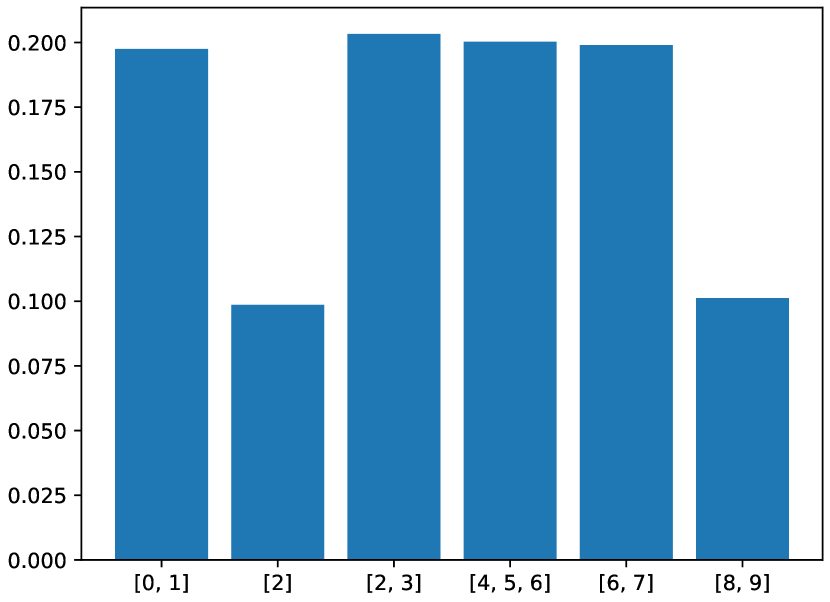
von Mises

Figure 1: Weights of the recovered couplings $u_{k}$ for the approximation of $f$ in (66) with a) and b) by the three mixture models in Example 2.3 for $N=10000$ samples. Top: model a), bottom: model b).

We observe that the couplings $u_{k}$ are reconstructed exactly. Further, the log likelihood value is for the sparse mixture model with full wrapped Gaussian covariance matrices in all cases larger than for the ground truth function. Thus, the approximation error is due to the estimation error of the maximum likelihood estimator and therefore due to the lack of information contained in the samples and not due to the approximation method. Further, the sparse mixture model with full wrapped Gaussian covariances admits in all cases a larger log likelihood value than those with the diagonal wrapped Gaussians. This should not be surprising, since the sparse mixture model with the wrapped Gaussian covariance matrices contains the other setting.

4.2 Samples from Functions

Next, we approximate the functions $f_{i}/\|f_{i}\|_{L^{1}}$, $i=1,2$, where $f_{1}\colon[0,1]^{9}\to\mathbb{R}$ and $f_{2}\colon[0,1]^{10}\to\mathbb{R}$ are given by

$$f_{1}(x) =B_{2}(x_{1})B_{4}(x_{3})B_{6}(x_{8})+B_{2}(x_{2})B_{4}(x_{5})B_{6}(x_{6})+B_{2}(x_{4})B_{4}(x_{7})B_{6}(x_{9}),$$ (67)

$$f_{2}(x) =10\sin(\pi x_{1}x_{2})+20(x_{3}+0.5)^{2}+10x_{4}+5x_{5}.$$ (68)

Here $B_{2}$, $B_{4}$ and $B_{6}$ are the $L_{2}$ normalized $B$-splines of order $2$, $4$ and $6$ supported on $[0,1]$. Note, that the spline function $f_{1}$ was also used in [4] for numerical evaluations. The function $f_{2}$ is the so-called Friedmann-1 function. We use $d_{s}=3$ iterations within the heuristic of Section 3.3 for $f_{1}$ and $d_{s}=2$ iterations for $f_{2}$. The results are given in Table 2. Figure 2 shows a diagram with the weights of the recovered couplings $u_{k}$. We observe that all recovered couplings $u_{k}$ with a significant weight match to the definitions of the functions $f_{i}$, $i=1,2$.

Method	$\mathcal{L}_{f}(x^{1},...,x^{N})$	$\mathcal{L}_{\hat{p}}(x^{1},...,x^{N})$	$e_{L^{1}}(\hat{p},f)$	$e_{L^{2}}(\hat{p},f)$
full	$7009.8\pm 59.4$	$7026.7\pm 79.2$	$0.0971\pm 0.0053$	$0.0963\pm 0.0056$
diagonal	$7009.8\pm 59.4$	$7001.9\pm 52.0$	$0.0828\pm 0.0030$	$0.0828\pm 0.0037$
von Mises	$7009.8\pm 59.4$	$6932.4\pm 56.4$	$0.1292\pm 0.0034$	$0.1272\pm 0.0041$

Method	$\mathcal{L}_{f}(x^{1},...,x^{N})$	$\mathcal{L}_{\hat{p}}(x^{1},...,x^{N})$	$e_{L^{1}}(\hat{p},f)$	$e_{L^{2}}(\hat{p},f)$
full	$630.0\pm 43.9$	$566.1\pm 43.0$	$0.1150\pm 0.0131$	$0.1419\pm 0.0142$
diagonal	$630.0\pm 43.9$	$558.6\pm 53.8$	$0.1175\pm 0.0135$	$0.1444\pm 0.0139$
von Mises	$630.0\pm 43.9$	$549.8\pm 56.4$	$0.1220\pm 0.0124$	$0.1490\pm 0.0128$

Table 2: Approximation of the $f_{i}$ in (67) and (68) by the three sparse mixture models in Example 2.3 for $N=10000$ samples. Average value of the log likelihood function and relative $L_{q}$, $q=1,2$. Top: Spline function $f_{1}$, bottom: Friedmann-1 function $f_{2}$.

wrapped

comp. wrapped

von Mises

Figure 2: Weights of the recovered couplings $u_{k}$ for the approximation of the $f_{i}$ in (67) and (68) by the three sparse mixture models in Example 2.3 for $N=10000$ samples. Top: Spline function $f_{1}$, bottom: Friedmann-1 function $f_{2}$.

The estimated parameters achieve a slightly worse log likelihood value than the original function $f$. Thus, the original function fits the samples slightly better than the estimated sparse mixture model. This should not be surprising, since the function $f/\|f\|_{L_{1}}$ is not contained in the class of sparse mixture models. Nevertheless, for the spline function $f_{1}$ the relative $L_{1}$ and $L_{2}$ errors are still comparable with the results from [4].

4.3 A Synthetic Image Example

In this example, we consider gray-valued images consisting of $7\times 10$ pixels which are sampled from five different classes. Each class contains noisy piece-wise constant images with one straight edge on a fixed position. In the following we learn a sparse mixture model for semi-supervised classification of images into one of these classes. Here we assume, that not the whole image is given, but only the orientations of some of the gradients within the images.

Image Generation

We generate an image $y=(y_{i,j})_{i,j}\in\mathbb{R}^{7\times 10}$ using the following procedure:

• Class 1: We draw $a$ from $\mathcal{N}(0.1,0.05^{2})$ and $b$ from $\mathcal{N}(0.9,0.1^{2})$ and set $y_{i,j}=a$ for $j=1,2$ and $y_{i,j}=b$ otherwise.

• Class 2: We draw $a$ from $\mathcal{N}(0.9,0.1^{2})$ and $b$ from $\mathcal{N}(0.1,0.05^{2})$ and set $y_{i,j}=a$ for $j=1,...,4$ and $y_{i,j}=b$ otherwise.

• Class 3: We draw $a$ from $\mathcal{N}(0.2,0.025^{2})$ and $b$ from $\mathcal{N}(0.6,0.05^{2})$ and set $y_{i,j}=a$ for $j=1,...,6$ and $y_{i,j}=b$ otherwise.

• Class 4: We draw $a$ from $\mathcal{N}(0.7,0.1^{2})$ and $b$ from $\mathcal{N}(0.1,0.05^{2})$ and set $y_{i,j}=a$ for $j=1,...,8$ and $y_{i,j}=b$ otherwise.

• Class 5: We draw $a$ from $\mathcal{N}(0.2,0.1^{2})$ and $b$ from $\mathcal{N}(0.9,0.025^{2})$ and set $y_{i,j}=a$ for $i=1,...,4$ and $y_{i,j}=b$ otherwise.

Finally, we add Gaussian white noise with standard deviation $0.2$ to each of the images. Figure 3 shows one sample from each class.

Figure 3: Three samples from each class.

Gradient Orientations and Data Generation

We assume that not the full images are given, but only the orientations of some of the gradients within the images. For an image $y=(y_{i,j})_{i,j}\in\mathbb{R}^{m\times n}$, the central discrete gradient at position $(i,j)\in\{2,...,m-1\}\times\{2,...,n-1\}$ is defined as the vector $(y_{i+1,j}-y_{i-1,j},y_{i,j+1}-y_{i,j-1})$. Consequently, the orientation of the gradient at position $(i,j)$ is given by

$$\omega_{i,j}\coloneqq\frac{1}{2\pi}\arctan^{*}(\tfrac{y_{i+1,j}-y_{i-1,j}}{y_{i,j+1}-y_{i,j-1}}),$$

where $\arctan^{*}$ again denotes the quadrant specific inverse of the tangent as defined in (36). Finally, we assume that not all of the gradient orientations are given, but only the $\omega_{ij}$ with $(i,j)\in\mathcal{I}$, where

$$\mathcal{I}\coloneqq\{(2,2),(2,3),(2,6),(2,7),(4,4),(4,5),(4,8),(4,9),(6,2),(6,3),(6,6),(6,7)\}.$$

Figure 4 visualizes the pixels corresponding to the positions $(i,j)\in\mathcal{I}$.

Figure 4: The black marked pixels represent the positions $(i,j)\in\mathcal{I}$.

Now, we generate $N_{\text{train}}=10000$ training samples and $N_{\text{test}}=1000$ test samples, where each sample $x\in\mathbb{T}^{12}$ is generated by the following steps: First, we choose randomly a class $c\in\{1,...,5\}$ accordingly to some fixed (but for the classification unknown) probabilities $\alpha$. Second, we generate an image $y$ from class $c$ as described above and compute the gradient orientations $\omega_{ij}$. Finally, we define our sample $x\in\mathbb{T}^{12}$ as $x\coloneqq(\omega_{ij})_{(i,j)\in\mathcal{I}}$.

We visualize the components of $(\omega_{ij})_{(i,j)\in\mathcal{I}}$ by histograms of $10000$ samples from class 2 in Figure 5.

Remark 4.1.

Let us briefly comment why the above sampling generation fits into our model setting. If the $Y_{i,j}$ are i.i.d. Gaussian distributed (noise on constant areas), then the components of their centered gradients are also i.i.d. Gaussian distributed for $(i,j)\in\mathcal{I}$. Note that the special set $\mathcal{I}$ is needed to ensure independence of the random variables in the gradient. Finally, it follows from the transformation theorem, that the random variable, where these $\omega_{i,j}$ are sampled from, are uniformly distributed, see e.g. [18]. Thus, in our samples $x$ most of the components will arise from a uniformly distributed random variable (constant areas) and only few ones (phases of the gradients at edges) must approximated by a Gaussian-like mixture.

Figure 5: Histograms of the components of $(\omega_{ij})_{(i,j)\in\mathcal{I}}$ for $10000$ samples from class 2.

Semi-Supervised Classification

In the following, assume that we have given $N_{\text{train}}$ unlabeled training samples $x^{1},...,x^{N_{\text{train}}}$ (i.e. it is unknown, which sample belongs to which class). Additionally, we have given $3$ labeled samples $x^{1,c},...,x^{3,c}$ from each class $c=1,...,5$. Based on this, we would like to classify the samples from the test set into the five classes. For this, we perform three steps.

• First, we estimate the components $u_{k}$ and the parameters $(\alpha,\mu,\Sigma)$ of a sparse mixture model as described in Section 3, where we use $d_{s}=4$ steps within the heuristic from Section 3.3.

• In general, this mixture model will have $K>5$ classes and we have to assign the components to the different classes. For this we assume that we have additionally given three labeled samples $x^{1,c},...,x^{3,c}$ from each class $c=1,...,5$. Then we assign $k$ to class $c(k)\in\{1,\ldots,5\}$ by

  $$c(k)\coloneqq\operatorname*{arg\,max}_{c=1,...,5}\sum_{i=1}^{3}\log\left(p_{u_{k}}(x^{i,c}_{u_{k}}|\vartheta_{k})\right).$$

• Finally, we predict for a data point $x$ from the test set the appropriate class

  $$\hat{c}\coloneqq\operatorname*{arg\,max}_{c=1,...,5}\sum_{k\in[K],c_{k}=c}\alpha_{k}p_{u_{k}}(x_{u_{k}}|\vartheta_{k}).$$

Using this procedure, we achieve an accuracy of $93.6\%$ on the test set.

Appendix A EM Algorithm for Distributions in Example 2.3

We summarize the EM algorithms for the mixture models with components from Example 2.3 i) - iii) in this order.

Algorithm 2 EM Algorithm for MMs with Wrapped Normal Distribution

Input: $x=(x^{1},...,x^{N})\in\mathbb{R}^{d,N}$, initialization $\alpha^{(0)}$, $\vartheta^{(0)}=(\mu^{(0)},\Sigma^{(0)})$.

for $r=0,1,...$ do

     E-Step: For $k=1,...,K$, $i=1,\ldots,N$ and $l\in\mathbb{Z}^{|u|}$ compute

$$\beta_{i,k,l}^{(r)} =\frac{\alpha_{k}^{(r)}\mathcal{N}(x^{i}_{u_{k}}+l|\mu_{k}^{(r)},\Sigma_{k}^{(r)}))}{\sum_{j=1}^{K}\alpha_{j}^{(r)}p(x^{i}_{u_{j}}|\mu_{j}^{(r)},\Sigma_{j}^{(r)})}$$ (69)

     M-Step: For $k=1,...,K$ compute

$$\alpha_{k}^{(r+1)} =\frac{1}{N}\sum_{i=1}^{N}w_{i}\sum_{l\in\mathbb{Z}^{|u_{k}|}}\beta_{i,k,l}^{(r)},$$ (70)

$$\mu_{k}^{(r+1)} =\frac{1}{N\alpha_{k}^{(r+1)}}\sum_{i=1}^{N}w_{i}\sum_{l\in\mathbb{Z}^{|u_{k}|}}\beta_{i,k,l}^{(r)}(x_{u_{k}}^{i}+l),$$ (71)

$$\Sigma_{k}^{(r+1)} =\frac{1}{N\alpha_{k}^{(r+1)}}\sum_{i=1}^{N}w_{i}\sum_{l\in\mathbb{Z}^{|u_{k}|}}\beta_{i,k,l}^{(r)}(x_{u_{k}}^{i}+l-\mu_{k}^{(r+1)})(x_{u_{k}}^{i}+l-\mu_{k}^{(r+1)})^{\mathrm{T}}.$$ (72)

end for

Algorithm 3 EM Algorithm for MMs with Diagonal Wrapped Normal Distribution

Input: $x=(x^{1},...,x^{N})\in\mathbb{R}^{d,N}$, initialization $\alpha^{(0)}$, $\vartheta^{(0)}=(\mu^{(0)},(\sigma_{j,k}^{(0)})^{2})$.

for $r=0,1,...$ do

     E-Step: For $k=1,...,K$, $i=1,\ldots,N$, $j\in u_{k}$ and $m\in\mathbb{Z}$ compute

$$\gamma^{(r)}_{i,k,m,j} =\frac{\alpha_{k}^{(r)}\mathcal{N}(x_{j}^{i}+m|\mu_{j,k}^{(r)},(\sigma_{j,k}^{(r)})^{2})\prod_{s\in u_{k}\backslash\{j\}}\mathcal{N}_{w}(x^{i}_{s}|\mu_{s,k}^{(r)},(\sigma_{s,k}^{(r)})^{2})}{\sum_{t=1}^{K}\alpha_{t}^{(r)}\prod_{s\in u_{t}}\mathcal{N}_{w}(x^{i}_{s}|\mu^{(r)}_{s,t},(\sigma^{(r)}_{s,t})^{2})}$$ (73)

     M-Step: For $k=1,...,K$ compute

$$\alpha_{k}^{(r+1)} =\frac{1}{N}\sum_{i=1}^{N}w_{i}\sum_{m\in\mathbb{Z}}\gamma_{i,k,m,j}^{(r)},\quad\text{for any }j\in u_{k}$$ (74)

$$\mu_{j,k}^{(r+1)} =\frac{1}{N\alpha_{k}^{(r+1)}}\sum_{i=1}^{N}w_{i}\sum_{m\in\mathbb{Z}}\gamma_{i,k,m,j}^{(r)}(x^{i}_{j}+m),$$ (75)

$$(\sigma_{j,k}^{(r+1)})^{2} =\frac{1}{N\alpha_{k}^{(r+1)}}\sum_{i=1}^{N}w_{i}\sum_{m\in\mathbb{Z}}\gamma_{i,k,m,j}^{(r)}(x^{i}_{j}+m-\mu_{j,k}^{(r+1)})^{2}.$$ (76)

end for

Algorithm 4 EM Algorithm for MMs with products of von Mises Distributions

Input: $x=(x^{1},...,x^{N})\in\mathbb{R}^{d,N}$, initialization $\alpha^{(0)}$, $\vartheta^{(0)}=(\mu_{j,k}^{(0)},\kappa_{j,k}^{(0)})$.

for $r=0,1,...$ do

     E-Step: For $k=1,...,K$, $i=1,\ldots,N$ compute

$$\beta^{(r)}_{i,k} =\frac{\alpha_{k}^{(r)}\prod_{j\in u_{k}}p_{M}(x^{i}_{j}|\mu_{j,k}^{(r)},\kappa_{j,k}^{(r)})}{\sum_{t=1}^{K}\alpha_{t}^{(r)}\prod_{j\in u_{t}}p_{M}(x^{i}_{j}|\mu^{(r)}_{j,t},\kappa^{(r)}_{j,t})}$$ (77)

     M-Step: For $k=1,...,K$ and $j\in u_{k}$ compute

$$\alpha_{k}^{(r+1)}=\frac{1}{N}\sum_{i=1}^{N}w_{i}\beta_{i,k}^{(r)},\quad\mu_{j,k}^{(r+1)}=\arctan^{*}\Big{(}\tfrac{S_{j,k}^{(r)}}{C_{j,k}^{(r)}}\Big{)},\quad\kappa_{j,k}^{(r+1)}=A^{-1}(R_{j,k}^{(r)}),$$ (78)

where

$$C_{j,k}^{(r)} =\sum_{i=1}^{N}w_{i}\beta_{ik}^{(r)}\cos(2\pi x^{i}_{j}),\quad S_{j,k}^{(r)}=\sum_{i=1}^{N}w_{i}\beta_{ik}^{(r)}\sin(2\pi x^{i}_{j}),$$ (79)

$$R_{j,k}^{(r)} =\tfrac{1}{N\alpha_{k}^{(r+1)}}\sqrt{(S_{j,k}^{(r)})^{2}+(C_{j,k}^{(r)})^{2}}.$$ (80)

end for

Appendix B The Weighted Kolmogorov-Smirnov Test

We briefly review the weighted Kolmogorov-Smirnov (KS) test. The following definition and facts about the KS test can be found in [45]. Given univariate samples $x^{1},...,x^{N}\in[0,1]$ and a probability distribution defined by its cumulative distribution function $f\colon[0,1]\to[0,1]$, we test the hypothesis

$$H_{0}\colon(x^{i})_{i}\text{ belong to the distribution }f$$

against the alternative

$$H_{1}\colon(x^{i})_{i}\text{ belong not to the distribution }f.$$

We define the empirical cumulative density function $f_{N}\colon[0,1]\to[0,1]$ of the samples $(x^{i})_{i}$ by

$$f_{N}=\frac{1}{N}\sum_{i=1}^{N}1_{[x^{i},1]}.$$

Then, the hypothesis $H_{0}$ is accepted, if the test statistic

$$\mathrm{KS}((x^{i})_{i})\coloneqq\sqrt{N}\|f_{N}-f\|_{L^{\infty}}$$ (81)

is smaller or equal than some constant $c$, which was fixed a priori and controls the significance level of the test. It is shown that for $X^{1},...,X^{N}$ i.i.d. random variables with cumulative distribution function $f$, the KS test statistic $\mathrm{KS}((X^{i})_{i})$ converges in distribution to the Kolmogorov distribution as $N\to\infty$.

The test can be extended for weighted samples $(w_{1},x^{1}),...,(w_{N},x^{N})\in\mathbb{R}_{>0}\times[0,1]$ by replacing the empirical cumulative distribution function by

$$f_{N}=\frac{1}{\sum_{i=1}^{N}w_{i}}\sum_{i=1}^{N}w_{i}1_{[x^{i},1]}.$$

Further, one has to replace $\sqrt{N}$ in (81). Here, [45] suggests to replace $N$ by $\frac{\big{(}\sum_{i=1}^{N}w_{i})\big{)}^{2}}{\sum_{i=1}^{N}w_{i}^{2}}$. Thus, the weighted KS test statistic reads as

$$\mathrm{KS}((w_{i},x^{i})_{i})=\sqrt{\frac{\big{(}\sum_{i=1}^{N}w_{i})\big{)}^{2}}{\sum_{i=1}^{N}w_{i}^{2}}}\|f_{N}-f\|_{L^{\infty}}.$$ (82)

Remark B.1.

Note that for two cumulative distribution functions $f$ and $g$ the term $d(f,g)=\|f-g\|_{L^{\infty}}$ defines a metric on the probability measures on $[0,1]$. In particular, for fixed weights $w_{i}$, the weighted KS test statistic can be interpreted as the distance of the measure induced by $f$ to the measure $\frac{1}{\sum_{i=1}^{N}w_{i}}\sum_{i=1}^{N}w_{i}\delta_{x^{i}}$, where $\delta_{x}$ is the Dirac-measure in $x$.

Remark B.2.

For the uniform distribution the weighted KS test statistic can be easily computed. Assume that the $x^{i}$ are sorted, i.e. $x^{1}\leq\cdots\leq x^{N}$, and denote by $s_{i}=\frac{\sum_{j=1}^{i}w_{j}}{\sum_{j=1}^{N}w_{j}}$. Then the (82) is given by

$$\mathrm{KS}((w_{i},x^{i})_{i})=\sqrt{\frac{\big{(}\sum_{i=1}^{N}w_{i})\big{)}^{2}}{\sum_{i=1}^{N}w_{i}^{2}}}\max_{i=1,...,N}\{\max(s_{i}-x_{i},x_{i}-s_{i-1})\}.$$

References

- [1] Y. Agiomyrgiannakis and Y. Stylianou. Wrapped Gaussian mixture models for modeling and high-rate quantization of phase data of speech. IEEE Transactions on Audio, Speech, and Language Processing, 17(4):775–786, 2009.
- [2] C. Andrieu, N. De Freitas, A. Doucet, and M. I. Jordan. An introduction to MCMC for machine learning. Machine learning, 50(1):5–43, 2003.
- [3] A. Banerjee, I. Dhillon, J. Ghosh, and S. Sra. Clustering on the unit hypersphere using von mises-fisher distributions. Journal of Machine Learning Research, 6:1345–1382, 09 2005.
- [4] F. Bartel, D. Potts, and M. Schmischke. Grouped transformations in high-dimensional explainable ANOVA approximation. arXiv preprint arXiv:2010.10199, 2020.
- [5] G. Beylkin, J. Garcke, and M. J. Mohlenkamp. Multivariate regression and machine learning with sums of separable functions. SIAM Journal on Scientific Computing, 31(3):1840–1857, 2009.
- [6] P. Binev, W. Dahmen, and P. Lamby. Fast high-dimensional approximation with sparse occupancy trees. Journal of Computational and Applied Mathematics, 235(8):2063–2076, 2011.
- [7] C. Bouveyron, S. Girard, and C. Schmid. High-dimensional data clustering. Computational Statistics & Data Analysis, 52(1):502–519, 2007.
- [8] J. Breckling. The analysis of directional time series: applications to wind speed and direction, volume 61 of Lecture Notes in Statistics. Springer-Verlag, Berlin, 1989.
- [9] C. L. Byrne. The EM Algorithm: Theory, Applications and Related Methods. Lecture Notes, University of Massachusetts, 2017.
- [10] R. Caflisch, W. Morokoff, and A. Owen. Valuation of mortgage-backed securities using Brownian bridges to reduce effective dimension. Journal of Computational Finance, 1:27–46, 1997.
- [11] R. Chitta, R. Jin, and A. K. Jain. Efficient kernel clustering using random Fourier features. 2012 IEEE 12th International Conference on Data Mining, pages 161–170, 2012.
- [12] S. Chrétien and A. O. Hero. Kullback proximal algorithms for maximum-likelihood estimation. IEEE Transactions on Information Theory, 46(5):1800–1810, 2000.
- [13] S. Chrétien and A. O. Hero. On EM algorithms and their proximal generalizations. ESAIM: Probability and Statistics, 12:308–326, 2008.
- [14] P. Constantine, E. Dow, and Q. Wang. Active subspace methods in theory and practice: Applications to kriging surfaces. SIAM Journal on Scientific Computing, 36, 2014.
- [15] P. Constantine, A. Eftekhari, J. Hokanson, and R. Ward. A near-stationary subspace for ridge approximation. Computer Methods in Applied Mechanics and Engineering, 326:402–421, 2017.
- [16] J. Delon and A. Desolneux. A Wasserstein-type distance in the space of Gaussian mixture models. SIAM Journal on Imaging Sciences, 13(2):936—970, 2020.
- [17] A. P. Dempster, N. M. Laird, and D. B. Rubin. Maximum likelihood from incomplete data via the EM algorithm. Journal of the Royal Statistical Society. Series B (Methodological), 39(1):1–38, 1977.
- [18] A. Desolneux, L. S., L. Moisan, and J.-M. Morel. Dequantizing image orientation. IEEE Transactions on Image Processing, 11(10):1129–1140, 2002.
- [19] R. DeVore, G. Petrova, and P. Wojtaszczyk. Approximation of functions of few variables in high dimensions. Constructive Approximation, 33:125–143, 2011.
- [20] N. Fisher. Problems with the current definitions of the standard deviation of wind direction. Journal of Applied Meteorology and Climatology, 26(11):1522–1529, 1987.
- [21] M. Fornasier, K. Schnass, and J. Vybíral. Learning functions of few arbitrary linear parameters in high dimensions. Foundations of Computational Mathematics, 12:229–262, 2012.
- [22] M. D. Fraser, Y.-S. Hsu, and J. J. Walker. Identifiability of finite mixtures of von Mises distributions. The Annals of Statistics, 9(5):1130–1131, 1981.
- [23] M. Goyal, M. Pandey, and R. Thakur. Exploratory analysis of machine learning techniques to predict energy efficiency in buildings. 2020 8th International Conference on Reliability, Infocom Technologies and Optimization (Trends and Future Directions) (ICRITO), pages 1033–1037, 2020.
- [24] R. Griboval, G. Balnchard, N. Keriven, and Y. Traonmilin. Compressive statistical learning with random feature moments. arXiv preprint arXiv:1706.07180v3, 2020.
- [25] C. Gu. Smoothing spline ANOVA models, volume 297 of Springer Series in Statistics. Springer, New York, second edition, 2013.
- [26] A. Hashemi, H. Schaeffer, R. Shi, U. Topcu, G. Tran, and R. Ward. Function approximation via sparse random features. arXiv preprint arXiv:2103.03191, 2021.
- [27] J. Hertrich, D. P. L. Nguyen, J.-F. Aujol, D. Bernard, Y. Berthoumieu, A. Saadaldin, and G. Steidl. PCA reduced Gaussian mixture models with applications in superresolution. arXiv preprint arXiv:2009.07520, 2020.
- [28] M. Holtz. Sparse grid quadrature in high dimensions with applications in finance and insurance. In Lecture Notes in Computational Science and Engineering, volume 77. Springer, 2011.
- [29] H. Holzmann, A. Munk, and B. Stratmann. Identifiability of finite mixtures - with applications to circular distributions. The Indian Journal of Statistics, 66:440–449, 2004.
- [30] A. Houdard, C. Bouveyron, and J. Delon. High-dimensional mixture models for unsupervised image denoising (HDMI). SIAM Journal on Imaging Sciences, 11(4):2815–2846, 2018.
- [31] S. R. Jammalamadaka and A. SenGupta. Topics in circular statistics, volume 5 of Series on Multivariate Analysis. World Scientific Publishing Co., Inc., River Edge, NJ, 2001.
- [32] D. G. Kendall. Pole-seeking Brownian motion and bird navigation. Journal of the Royal Statistical Society: Series B (Methodological), 36(3):365–402, 1974.
- [33] Y. Kokkinos and K. Margaritis. Multithreaded local learning regularization neural networks for regression tasks. In EANN, page 129—138. Springer International Publishing, 2015.
- [34] F. Y. Kuo, I. H. Sloan, G. W. Wasilkowski, and H. Woźniakowski. On decompositions of multivariate functions. Mathematics of Computation, 79(270):953–966, 2010.
- [35] G. Kurz, I. Gilitschenski, and U. D. Hanebeck. Efficient evaluation of the probability density function of a wrapped normal distribution. In 2014 Sensor Data Fusion: Trends, Solutions, Applications (SDF), pages 1–5. IEEE, 2014.
- [36] F. Laus. Statistical Analysis and Optimal Transport for Euclidean and Manifold-Valued Data. PhD Thesis, TU Kaiserslautern, 2019.
- [37] Z. Li, J.-F. Ton, D. Oglic, and D. Sejdinovic. Towards a unified analysis of random Fourier features. In International Conference on Machine Learning, pages 3905–3914, 2019.
- [38] R. Liu and A. Owen. Estimating mean dimensionality of analysis of variance decompositions. Journal of the American Statistical Association, 101:712 – 721, 2006.
- [39] K. Mardia and P. Jupp. Directional Statistics. Wiley Series in Probability and Statistics. Wiley, 2009.
- [40] K. V. Mardia. Bayesian analysis for bivariate von Mises distributions. Journal of Applied Statistics, 37(3):515–528, 2010.
- [41] K. V. Mardia, G. Hughes, C. C. Taylor, and H. Singh. A multivariate von Mises distribution with applications to bioinformatics. Canadian Journal of Statistics, 36(1):99–109, 2008.
- [42] K. V. Mardia, C. C. Taylor, and G. K. Subramaniam. Protein bioinformatics and mixtures of bivariate von Mises distributions for angular data. Biometrics, 63(2):505–512, 2007.
- [43] G. McLachlan and D. Peel. Finite Mixture Models. Wiley Series in Probability and Statistics. Wiley, 2004.
- [44] D. Meyer, F. Leisch, and K. Hornik. The support vector machine under test. Neurocomputing, 55(1):169–186, 2003.
- [45] J. F. Monahan. Numerical methods of statistics, volume 7 of Cambridge Series in Statistical and Probabilistic Mathematics. Cambridge University Press, Cambridge, second edition, 2011.
- [46] D. Potts and M. Schmischke. Interpretable approximation of high-dimensional data. arXiv preprint arXiv:2103.13787, 2021.
- [47] D. Potts and M. Schmischke. Learning high-dimensional periodic functions with Fourier based methods. arXiv preprint arXiv:1907.11412, 2021.
- [48] A. Rahimi and B. Recht. Random features for large-scale kernel machines. In Advances in Neural Information Processing Systems, volume 20, 2008.
- [49] C. P. Robert and G. Casella. Monte Carlo statistical methods. Springer Texts in Statistics. Springer-Verlag, New York, second edition, 2004.
- [50] H. Shi, Y. Traonmilin, and J.-F. Aujol. Sketched learning for image denoising. In A. Elmoataz, J. Fadili, Y. Quéau, J. Rabin, and L. Simon, editors, Scale Space and Variational Methods, volume 12679 of Lecture Notes in Computer Science, pages 281–293. Springer, 2021.
- [51] P. Smaragdis and P. Boufounos. Learning source trajectories using wrapped-phase hidden Markov models. In IEEE Workshop on Applications of Signal Processing to Audio and Acoustics, 2005., pages 114–117. IEEE, 2005.
- [52] H. Teicher. Identifiability of mixtures. The Annals of Mathematical Statistics, 32(1):244–248, 1961.
- [53] H. Teicher. Identifiability of mixtures of product measures. The Annals of Mathematical Statistics, 38(4):1300–1302, 1967.
- [54] M. E. Tipping and C. M. Bishop. Mixtures of probabilistic principal component analyzers. Neural Computation, 11(2):443–482, 1999.
- [55] C. F. J. Wu and M. S. Hamada. Experiments: planning, analysis, and optimization. Wiley Series in Probability and Statistics. John Wiley & Sons, Inc., Hoboken, NJ, second edition, 2009.
- [56] S. J. Yakowitz and J. D. Spragins. On the identifiability of finite mixtures. The Annals of Mathematical Statistics, pages 209–214, 1968.
- [57] T. Yang, Y.-F. Li, M. Mahdavi, R. Jin, and Z. Zhou. Nyström method vs random Fourier features: A theoretical and empirical comparison. Advances in Neural Information Processing Systems, 25:476–484, 2012.