Myocardial ischemic effects on cardiac electro-mechanical activity

Abstract

In this work, we investigated the effect of varying strength of Hyperkalemia and Hypoxia, in a human cardiac tissue with a local ischemic subregion, on the electrical and mechanical activity of healthy and ischemic zones of the cardiac muscle. The Monodomain model in a deforming domain is taken with the addition of mechanical feedback and stretch activated channel current coupled with the ten Tusscher human ventricular membrane model. The equations of finite elasticity are used to describe the deformation of the cardiac tissue. The resulting coupled electro-mechanical PDEs-ODEs non-linear system is solved numerically using finite elements in space and finite difference method in time. We examined the effect of local ischemia on the cardiac electrical and mechanical activity in different cases. We concluded that the spread of Hyperkalemic or Hypoxic region alters the electro-mechanical coupling in terms of the action potential ($v$), intracellular calcium ion concentration $[Ca^{+2}]_{i}$, active tension, ($T_{A}$), stretch ($\lambda$), stretch rate ($\frac{d\lambda}{dt}$). With the increase in the size of the ischemic region by factor of five, approximately $45\%$ variation in the stretch rate $\frac{d\lambda}{dt}$ is noticed. It is also shown that ischemia affects the deformation (expansion and contraction) of the heart.

1 Introduction

The heart is considered as a muscular pump which is connected to the systemic and pulmonary vascular systems. The main purpose of the heart and vascular system is to sustain an appropriate supply of nutrients as oxygenated blood and metabolic substrates to the body. The left atrium and ventricle chambers pump the blood from pulmonary veins to the aorta, whereas the right atrium and ventricle chambers pump the blood from vena cava to pulmonary arteries. The cardiac cycle consists of two phases: diastole, during which the ventricles relax and the heart fills with blood; and systole, during which the ventricles contract and pump blood out of the heart to arteries. To this end, the heart needs three types of cells: 1. SA node or pacemaker cells, which produce an electrical signal; 2. Conductors to spread the pacemaker signals; and 3. Contractile cells, to mechanically pump blood. Pacemaker cells start the electrical sequence of depolarization and repolarization. The electrical signal generated from the SA node travels to the ventricles via the atrioventricular node(AV node), the bundle of His, the right and left bundle branches and Purkinje fibers. As the depolarization signal reaches the contractile cells they start to contract and as the repolarization signal reaches the myocardial cells, they start to relax. In this way the electrical signals and the mechanical pumping action of the heart are connected via excitation-contraction coupling. Heart’s electrical and mechanical activity can be deduced from the ECG pattern. P wave represents the atrial depolarization, QRS complex due to the ventricular depolarization also start of the ventricular contraction, T wave indicate the ventricular repolarization and the beginning of ventricular relaxation.

There exist one factor, called stretch, which is responsible for the activation and inactivation of the mechanically controlled ion channels. In 1997, Hu & Sachs [HS97] revealed the stretch activated channels (SACs) in cardiac cells. Positive response of the SACs contribute for heart to stretch. Cardiac muscle stretch also leads to the increase in active tension.

For the finite elasticity material, there are various models for the strain energy function based on the different laws. For example, in [GCM95a] Guccione et al. used the transversely isotropic exponential law strain energy function and the orthotropic and isotropic laws have been used in [NP04] and [CBP⁺14a], respectively. Various models for the development of the active tension and the description of the dynamics of calcium ions and the cross bridges bindings have been proposed in [CBP⁺14b, DGKK13, EPPH13, KNP09, KOMM10, MW07, RLRB⁺14, SMCCS06, WGRS11, PW09, LNA⁺12a, JGT10, GLC⁺11, GCRT10, DORB⁺13, CHLT13, AHZ13a]. In [HMTK98], Hunter et al. presented the model based on the review of experimental data for the mechanics of active and passive cardiac muscle. They concluded that it could be interpreted as the four state variable model. (i) myocardial tissue passive elasticity, (ii) tension dependence on the troponin C and $Ca^{+2}$ bindings, (iii) tropomyosin movement kinetics and the actively cycling cross-bridges binding sites and the length dependence of this process, and, (iv) cross-bridge tension development kinetics under variations of the myofilament length. In [NS07], developed a biophysically and dynamically stable model for the cardiac myocyte of rat at the room temperature. This model is capable of determining the changes in the concentration of intracellular calcium ion in response to the stretch. In [LNA⁺12b], presented a multiscale electro-mechanical model for the murince heart which is capable of investigating the effects of excitation-contraction coupling. In this paper,they show a strong relation between the tension and the velocity to explain the differences between the single cell tension and the whole organ pressure transient.

For the cardiac electrical activity models at the tissue level, Bidomain and Monodomain models have been considered in various researches [CHLT13, DORB⁺13, GCRT10, JGT10, WGRS11, DGKK13, MW07, RLRB⁺14, EPPH13, KNP09, KOMM10]. For the ionic membrane models related to the different species has been used in [CHLT13, DORB⁺13, GCRT10, JGT10, WGRS11, DGKK13, KNP09, KOMM10, MW07, RLRB⁺14, EPPH13] etc.

Following the electro-mechanical coupling approach presented in [AHZ13a, DORB⁺13, GCRT10, WBG07, RLRB⁺14, PCGW10, NQRB12, PW09, NSH05, KNP09, GK10a, DGKK13, AANQ11] we need to impose the electrical models on the deformed domain to propose the coupling between the electrical and mechanical model. Then by the Lagrangian framework again this model is reformulated into the reference domain.

There exist coupled cardiac electro-mechanical models which explain the traveling of electric signal into the cardiac muscle and the contraction-relaxation process. These models consists : 1) the electrical model at the tissue, which consists, the system of non-linear parabolic reaction-diffusion equations of the degenerate type, 2) the cell level model to describe the flow of ionic currents via cellular membrane consist, system of ordinary differential equations (ODEs), 3) deformation of cardiac tissue is modeled by the quasi-static finite elasticity model, 4)intracellular calcium dynamics and the cross bridges bindings are described by the active tension model which consists of a system of non-linear ODEs. Existence and uniqueness for the coupled electro-mechanical model is given in [ABQRB15, BMST18].

Cardiac arrhythmia involves the abnormality in the pattern of the heartbeat, if the electrical impulse fails to start from the SA node or if there is some abnormality in the impulse initiated from the SA node. Myocardial ischemia takes place when there is abnormality in the blood flow to heart and in oxygen supply to the heart. It is one of the main causes of sudden death. Cardiac arrhythmia and heart attack can also occur due to the myocardial ischemia. Due to this myocardial ischemia metabolism, electrophysiological and mechanical changes appear which results in the reduction of action potential duration (APD), action-potential upstroke, resting-potential shift, reduction in conduction velocity (CV), active tension, stretch along the fiber and the stretch rate in the ischemic cells or tissue [2, 3, 4].

Various experimental and numerical simulation work have been carried out to analyze the electrophysiological and metabolic properties of the healthy and ischemic cells and tissue [DMZ⁺16, JW89, PC87, TRET07, CFPS07, RHR⁺08]. Mathematical and computational studies have been focused on investigating various physiological effects in order to understand the relationship between the electrophysiological and metabolic parameters. It can be analyzed from the past studies that these variations are basically due to, a) Hyperkalemia which affects the cardiac cell resting potential due to the increase in the concentration of extracellular potassium [SSCF90, PWM⁺10], b) Hypoxia defined as the reduced oxygen supply, it reduces the cell metabolism and ADP to ATP concentration ratio in the cell get changed. Successively, this change affects the opening of the particular ATP-dependent potassium channels [WL94, WVL92]. This ATP-dependent potassium channels is also modulated by the mechanical environment.

There are several research papers in which they have studied about ischemia in the animals. [FBS⁺85, Car99, FKF⁺91, Cor94, MW07, PKZ⁺11, WTJC⁺86, SSCF90]. Since it is difficult to get the human data, and hence it is challenging to extend the properties from animals to human. But it can be achieved via computational modeling. Even though many human models have been built and analyzed via healthy cell data their appropriateness for the ischemia computation is not known. So, it is essential to examine the effect of varying ischemic parameters in the ischemic region. In [AP96, STO⁺00, TSO⁺00], studies have been done for the global ischemia in human under different ischemic conditions. In [PKP19], the authors has discussed the effect of local cardiac ischemia on the electrical activity of the ischemic region and the neighboring healthy region in a human cardiac tissue.

For the electro-mechanical coupling models, the bio-electrical activity experiences three main feedback from the mechanical deformation:

1. conductivity feedback: the influence of the deformation gradient on the conductivity coefficients of the electric current flow model;

2. convection feedback: the influence of deformation gradient and deformation rate on the electric current flow model;

3. ionic feedback: the influence of stretch-activated membrane channels on the ionic current.

In [CFPS16] authors considered these three cases together and study their effects in a strongly coupled anisotropic cardiac electro-mechanical model. X. Jie et al. [JGT10] used a electromechanical model for the ventricle of rabbit to analyze the arrhythmia originates from the ischemia induced electrophysiological and the mechanical changes. As per our literature survey no one has considered the electro-mechanical model of the human cardiac tissue to analyze the local ischemia effects on the electro-mechanical activity.

In this study, we will discuss the influence of local ischemic region on electrical and mechanical activity in the deforming human heart. For the electrical activity at cell level, we will use the ten Tusscher human ventricular membrane model [TTNNP04]. We will consider the above three cases (i), (ii), (iii) and study the effect in deformed Monodomain model. We will also show the effect of ischemia on this model. We will discuss the two types of ischemia namely Hyperkalemia and Hypoxia. We will discuss the influence of these two types of local ischemia, by changing the corresponding parameters in the 2D tissue level model, on the electrical and mechanical activity in terms of the action potential (AP), activation time (AT), repolarization time (RT), action potential duration (APD) and intracellular calcium ion concentration $[Ca^{+2}]_{i}$, active tension, ($T_{A}$), stretch ($\lambda$), stretch rate ($\frac{d\lambda}{dt}$). We will also see the effect of the spread of ischemic zone in both the ischemic subregion and the healthy region on the electrical and mechanical properties.

In the next section, we will describe the cardiac electro-mechanical model and also discuss about the ischemic parameters. We will also present the modeling of local ischemic zone. In the next section, we will present the fully discrete system using finite elements in space and backward Euler method in time. In section 4, we will discuss the numerical results.

2 Electro-mechanical models of cardiac tissue

Cardiac electro-mechanical model is a combination of electrical and mechanical models. In this section, we will describe the mechanical and electrical models of cardiac tissue.

2.1 Cardiac tissue mechanical model

Let $\hat{\Omega}$ is the undeformed cardiac domain and $\Omega(t)$ is the deformed cardiac domain at time ${}^{\prime}t^{\prime}$ with $X=(X_{1},X_{2})$ and $x=(x_{1},x_{2})$ are the spatial coordinates respectively.

Define the deformation map, $\psi_{t}(X)=\psi(X,t)=x$ from $\hat{\Omega}$ to $\Omega(t)$ and $u(X,t)=x-X$ as the displacement vector.

In this work, cardiac tissue is considered as a nonlinear elastic material.
The deformation gradient tensor$F(X,t)=\{F_{i,j}\}=\{\frac{\partial x_{i}}{\partial X_{j}},i,j=1,2,3\}$,
$J(X,t)=detF(X,t)$
Cauchy-Green deformation tensor $C=F^{T}F$,
Lagrange-Green strain tensor $\epsilon=\frac{1}{2}(C-1)$.
Also the deformed body satisfy the following steady state force equilibrium equation described as

$$div(FS(u,X))=0,X\in\hat{\Omega},$$ (1)

where $S$ is the second Piola-Kirchoff stress tensor. Prescribed displacement is imposed on the Dirichlet boundary $x(X,t)=\hat{x}(X),X\in\hat{\partial\Omega_{d}}$ and Neumann boundary with no traction force $n^{t}FS(u(X,t),X)=0,X\in\hat{\partial\Omega_{n}}$.

The second Piola-Kirchoff stress tensor $S$, as taken in the studies [HMTK98, KBK⁺03, VM00, CFPS16], is the combination of three components namely,

$$S=S^{A}+S^{P}+S^{V},$$

where active component $S^{A}$ generated biochemically, passive elastic component $S^{P}$ and volumetric component $S^{V}$.

Next, $S^{P,V}$ is defined as follows

$$S_{ij}^{P,V}=\frac{1}{2}\bigg{(}\frac{\partial W^{P,V}}{\partial\epsilon_{ij}}+\frac{\partial W^{P,V}}{\partial\epsilon_{ji}}\bigg{)},i,j=1,2,$$ (2)

where $W^{P,V}$ are the passive and volumetric strain energy functions, variety of these has been proposed in [CHM01, GCM95b, HO09, GK10b, SNCH00, RNH05, SNYH06, UMM00] and $\epsilon$ is the Green-Lagrange strain.

In this work, cardiac tissue is modeled as an orthotropic hyperelastic material. The passive strain energy function for a hyperelastic material is given as in [EPPH13]:

$$W^{P}=\frac{1}{2}(e^{Q}-1),$$

$$Q=\sum_{i=l,t}b_{i}(I_{4i}-1)^{2}+b_{lt}I_{8lt}^{2},$$

where $I_{4l}=\hat{b}_{l}^{T}C\hat{b}_{l}$, $I_{4t}=\hat{b}_{t}^{T}C\hat{b}_{t}$ and $I_{8lt}=\hat{b}_{l}^{T}C\hat{b}_{t}$,

and volumetric strain energy function for a hyperelastic material is given as

$$W^{V}=K(J-1)^{2},$$

where $K$ is a positive bulk modulus.

Now, the active component of second Piola-Kirchoff stress tensor $S^{A}$ is defined in the form of active tension originated along the myocytes.

An isometric contraction of the cardiac tissue, generates an active tension without changing length of the cardiac tissue. Mechanical model of active tension is modeled by the myofilaments dynamics activated by calcium. We consider, as suggested in [CFPS16], that the active force moves only in the fiber direction. Therefore, active Cauchy stress is given as

$$\sigma^{A}(x,t)=J^{-1}T_{A}a_{l}(x)\otimes a_{l}(x),$$ (3)

where $a_{l}=\frac{F\hat{a}_{l}}{|F\hat{a}_{l}|}$ is a unit vector parallel to the local fiber direction and $T_{A}$ is the active tension in the deformed domain.

The active component of second Piola-Kirchoff stress tensor $S^{A}$ is defined as

$$S^{A}=JF^{-1}\sigma^{A}F^{-T},$$ (4)

and the stretch rate along the fiber is defined as

$$\lambda=\sqrt{\hat{a}_{l}^{T}C\hat{a}_{l}}.$$ (5)

The active tension is dependent on calcium dynamics, stretch and stretch rate i.e. $T_{A}=T_{A}(Ca_{i},\lambda,\frac{d\lambda}{dt})$, as discussed in [LNA⁺12b] is given by the system of ODEs:

$$\frac{d(trpn)}{dt}=k_{trpn}\bigg{(}\bigg{(}\frac{Ca_{i}}{Ca_{50}(1+\beta(\lambda-1))}\bigg{)}^{n_{trpn}}\bigg{)},$$

$$\frac{dXb}{dt}=k_{Xb}\bigg{(}(trpn_{50})(trpn)^{n_{Xb}}(1-Xb)-\frac{1}{(trpn_{50})(trpn)^{n_{Xb}}}Xb\bigg{)},$$

$$\frac{dq_{i}}{dt}=A_{i}\frac{d\lambda}{dt}-\alpha_{i}q_{i},i=1,2,$$

$$T_{A}=g(q)h(\lambda)Xb,q=q_{1}+q_{2}.$$ (6)

where, function $g(q)$ is the effect on tension is defined as :

$$g(q)=\left\{\begin{array}[]{ll}\frac{aq+1}{1-q}&q\leq 0\\ \frac{1+(a+2)Q}{1+q}&q>0\\ \end{array}\right.$$

.

For more details refer to [LNA⁺12b].

2.2 Cardiac tissue electrical model on a deforming domain: Monodomain model

We assume that the cardiac tissue is insulated. The influence of the cardiac tissue deformation on the Monodomain model in the strong coupling framework is due to three different mechano-electrical feedback: a) presence of deformation gradient $F$ in the conductivity coefficients structure, b) presence of deformation gradient $F$ and the deformation rate in the conductive term, and c) presence of stretch $\lambda$ in the $I_{ion}$.

Monodomain model on the deformed domain $\Omega(t)$ is defined as follows:

$$\frac{\partial v}{\partial t}-div(D(x)\nabla v)+I_{ion}(v,w,c,\lambda)=I_{app},x\in\Omega(t),0\leq t\leq T$$ (7)

$$\frac{\partial w}{\partial t}-g(v,w)=0,x\in\Omega(t),0\leq t\leq T$$ (8)

$$\frac{\partial c}{\partial t}-f(v,w,c)=0,x\in\Omega(t),0\leq t\leq T$$ (9)

$$v(x,0)=v_{0}(x,0),\hskip 14.22636ptw(x,0)=w_{0}(x,0),\hskip 14.22636ptc(x,0)=c_{0}(x,0),x\in\Omega$$ (10)

$$n^{T}D(x)\nabla v=0,x\in\partial\Omega,0\leq t\leq T$$ (11)

where,

$$D(x)={\sigma_{l}}a_{l}(x){a_{l}}^{T}(x)+{\sigma_{t}}a_{t}(x){a_{t}}^{T}(x),$$

where, $a_{l}(x)$ is a unit vector along the local fiber direction and $a_{t}(x)$ is a unit vector transverse to the fiber direction and they both are orthogonal to each other. $\sigma_{l}$ and $\sigma_{t}$ are the conductivity coefficients in the corresponding directions.

$$D(x)={\sigma_{t}}I+({\sigma_{l}}-{\sigma_{t}})a_{l}(x){a_{l}}^{T}(x).$$

Let $\hat{v}(X,t),\hat{w}(X,t),\hat{c}(X,t)$ and $\hat{D}(X,t)$ are the action potential, gating, concentration variables on the undeformed domain $\hat{\Omega}$. Then

$$\frac{\partial\hat{v}}{\partial t}=\frac{\partial v}{\partial t}+\nabla v.\frac{\partial\psi_{t}}{\partial t},(\text{convective term})$$

$$\nabla v(x,t)=F^{-T}Grad\hat{v}(X,t),$$

$$dx=JdX,$$

Thus the monodomain system on the reference domain $\hat{\Omega}$ is given as follows:

$$J\bigg{(}\frac{\partial\hat{v}}{\partial t}-F^{-T}\nabla\hat{v}.\frac{d\psi_{t}}{dt}\bigg{)}-div(JF^{-1}DF^{-T}\nabla\hat{v})+JI_{ion}(\hat{v},\hat{w},\hat{c},\lambda)=JI_{app},\hskip 20.00003ptX\in\hat{\Omega},$$

coupled with the system of ODEs for the gating and concentration variables $w(x,t)$ and $c(x,t)$ respectively, given by

$$\frac{\partial w}{\partial t}-g(v,w)=0, X\in\hat{\Omega},T$$ (12)

$$\frac{\partial c}{\partial t}-f(v,w,c)=0, X\in\hat{\Omega}.$$ (13)

Initial conditions:

$$\hat{v}(X,0)=\hat{v}_{0}(X),\hskip 5.69054ptX\in\hat{\Omega},$$

$$w(X,0)=w_{0}(X),\hskip 14.22636ptc(X,0)=c_{0}(X),\hskip 2.84526ptX\in\hat{\Omega}.$$ (14)

Boundary condition:

$$n^{T}F^{-1}D(x)F^{-T}\nabla\hat{v}=0,\hskip 14.22636pt\text{on}\hskip 14.22636pt\partial\hat{\Omega}\times(0,T).$$ (15)

Now, we compute the conductivity tensor $\hat{D}(X,t)$ on the reference domain is given as:

$$\hat{D}(X,t)=F^{-1}D(x(X,t))F^{-T}(X,t),\hskip 22.76219ptX\in\hat{\Omega}$$

We know the conductivity tensor in the deformed domain $\Omega(t)$ is defined as

$$D(x)={\sigma_{t}}I+({\sigma_{l}}-{\sigma_{t}})a_{l}(x){a_{l}}^{T}(x).$$

Now, let $\hat{a}_{l}(X)$ is a unit vector parallel to the local fiber direction in the reference domain, then in the deformed domain the unit vector $a_{l}(x)$ along the local fiber direction is obtained by

$$a_{l} =\frac{F\hat{a}_{l}}{\|F\hat{a}_{l}\|},$$

$$=\frac{F\hat{a}_{l}}{\sqrt{\hat{a}_{l}^{T}C\hat{a}_{l}}}$$

Thus,

$$a_{l}a_{l}^{T}=\frac{F\hat{a}_{l}\hat{a}_{l}^{T}F^{T}}{{\hat{a}_{l}^{T}C\hat{a}_{l}}}$$

2.3 Ionic model

$I_{ion}(v,w,c,\lambda)$, $g(v,w)$ and $f(v,w,c)$ are defined by the cell level model. In this work we are using the human ventricular cell level model, ten Tusscher model [TTNNP04] (TT06). Dynamics of the ionic currents is modeled by the 17 ODEs. The ionic current flow $I_{sac}$ due to the stretch activated channels and $K_{ATP}$ current is also taken into account. Thus the total ionic current is given by

$$I_{ion}=I_{Na}+I_{K1}+I_{to}+I_{Kr}+I_{Ks}+I_{CaL}+I_{NaCa}+I_{NaK}+$$

$$\hskip 17.07182ptI_{pCa}+I_{pK}+I_{bCa}+I_{bNa}+I_{KATP}+I_{sac},$$ (16)

where, the fast sodium $(I_{Na})$, L-type calcium$(I_{CaL})$, transient outward$(I_{to})$ , rapid delayed rectifier$(I_{Kr})$ and slow delayed rectifier $(I_{Ks})$, and inward rectifier currents $(I_{K1})$, $I_{NaCa}$ is $Na/Ca^{2+}$ exchange current, $I_{NaK}$ is $Na/K^{+}$ pump current, $I_{pCa}$ and $I_{pK}$ are plateau $Ca^{2+}$ and $K^{+}$ currents, $I_{bCa}$ and $I_{bK}$ are background $Ca^{2+}$ and $K^{+}$ currents and $I_{KATP}$ is the$K_{ATP}$ current, all are modeled as in [TTNNP04], $I_{KATP}$ which accounts for Hypoxia is defined as in [AP96]:

$$I_{KATP}=G_{KATP}f_{ATP}\bigg{(}\frac{[K^{+}]_{o}}{5.4}\bigg{)}^{0.3}\frac{1}{40+3.5e^{0.025v}}(v-E_{k}),$$ (17)

where, $G_{KATP}$ is the conductance and $E_{k}$ is the resting potential of potassium.

$I_{sac}$, the stretch activated current [AHZ13b] is given as follows :

$$I_{sac}=I_{sac,n}+I_{Ko},$$

$$I_{sac,n}=I_{sac,Na}+I_{sac,K},$$

where, $I_{sac,n}$ is the non-specific current defined as follows:

$$I_{sac,Na}=G_{sac}\gamma_{slsac}(v-v_{Na})\bigg{(}-\frac{v_{R}+85}{v_{R}-65}\bigg{)},$$

$$I_{sac,K}=G_{sac}\gamma_{slsac}(v-v_{K}).$$

The specific $K^{+}$ stretch-dependent current is given by

$$I_{Ko}=G_{Ko}\frac{\gamma_{sl,Ko}}{1+exp(-(10+v)/45)}(v-v_{K}),$$

where, $\gamma_{sl,Ko}=3(\lambda-1)+0.7$.

The two types of ischemia, Hyperkalemia and Hypoxia will be incorporated into the model by varying the parameters corresponding to each of the two types of ischemia.

Human Cardiac tissue is considered as a square $ABCD$, and the ischemic region is taken as a small square $A_{1}B_{1}C_{1}D_{1}$. In this study, local ischemia is modeled by varying the ischemic parameter value in the sub-domain $A_{1}B_{1}C_{1}D_{1}$ only and using the normal value of the parameter in the remaining part of the cardiac tissue $ABCD$. Also considering the ischemia as mild, moderate and severe by taking the $[K^{+}]_{o}$ parameter value in the corresponding range in the domain $A_{1}B_{1}C_{1}D_{1}$ only. Then, we compare the electrophysiological properties of the ischemic and non-ischemic region points say $(x,y)$ and $(x^{\prime},y^{\prime})$ respectively (see Fig.(1)).

Figure 1: : Cardiac tissue $ABCD$ with single ischemic subregion $A1B1C1D1$, $(x,y)$ and $(x^{\prime},y^{\prime})$ are the points inside and outside the ischemic subregion.

3 Weak Formulation

First of all we define the strong form the model. Monodomain model on the deformed domain $\Omega(t)$ is defined as follows:

(elasticity equation) $$-\nabla.(\nabla u\sigma(x,\gamma))=f, x\in\Omega(t),a.e.t\in(0,T)$$ (18)

(Tissue level model) $$\frac{\partial v}{\partial t}-div(D(x)\nabla v)+I_{ion}(v,w,c,\lambda)=I_{app}, x\in\Omega(t),0\leq t\leq T$$ (19)

(cell level model) $$\frac{\partial w}{\partial t}=G(v,w), x\in\Omega(t),0\leq t\leq T$$ (20)

$$\frac{\partial c}{\partial t}=h(v,w,c), x\in\Omega(t),0\leq t\leq T$$ (21)

$$\frac{\partial\gamma}{\partial t}=S(\gamma,w), x\in\Omega(t),0\leq t\leq T$$ (22)

$$v(x,0)=v_{0}(x,0),\hskip 5.69054ptw(x,0)=w_{0}(x,0),\hskip 5.69054ptc(x,0)=c_{0}(x,0), x\in\Omega(t)$$ (23)

$$n^{T}D(x)\nabla v=0, x\in\partial\Omega,0\leq t\leq T.$$ (24)

Now, we will define the general form of the ionic model so that the weak formulation of the above model equations can be written.

The general form of ionic current $I_{ion}:\mathbb{R}\times\mathbb{R}^{d}\times(0,\infty)^{n}\to\mathbb{R}$ is defined as follows:

$$I_{ion}(v,w,c):=\sum_{i=1}^{n}Q_{i}(v,w,logc_{i})+R(v,w,c),$$ (25)

where,

$$Q_{i}\in C^{1}(\mathbb{R}\times\mathbb{R}^{d}\times\mathbb{R}),$$

$$0<\underline{\rm H}(w)\leq\frac{\partial}{\partial\zeta}Q_{i}(v,w,\zeta)\leq\overline{\rm H}(w),$$

$$|\frac{\partial}{\partial v}Q_{i}(v,w,0)|\leq L(w),$$ (26)

$\underline{\rm H},\overline{\rm H},L\in C^{0}(\mathbb{R}^{d},\mathbb{R}_{+})$ and

$$R\in C^{0}(\mathbb{R}\times\mathbb{R}^{d}\times(0,\infty)^{n})\cap Lip(\mathbb{R}\times[0,1]^{d}\times(0,+\infty)^{m}).$$ (27)

The following system of ODEs describing the dynamics of gating variables,

$$\frac{\partial w_{i}}{\partial t}=G_{i}(v,w_{i}),\hskip 14.22636pti=1,2,...,d.$$ (28)

where, $G_{i}$ has the particular form as

$$G_{i}(v,w):=\alpha_{i}(v)(1-w_{i})-\beta_{i}(v)w_{i},\hskip 14.22636pti=1,2,...,d,$$

and $\alpha_{i}$ and $\beta_{i}$ are positive rational exponential functions in $v$.

Assumption, $\forall\hskip 5.69054pti=1,2,...,d$,

$$G_{i}:\mathbb{R}^{2}\to\mathbb{R}\hskip 14.22636pt\textbf{is locally Lipschitz continuous},$$

$$G_{i}(v,0)\geq 0\hskip 14.22636pt\forall v\in\mathbb{R},$$

$$G_{i}(v,1)\leq 0\hskip 14.22636pt\forall v\in\mathbb{R}.$$ (29)

ODEs describing the dynamics of concentration variables is given by

$$\frac{\partial c_{j}}{\partial t}=h_{j}(v,w,c_{j}):=Q_{j}(v,w,c_{j})+R_{j}(v,w,c_{j}),\hskip 14.22636ptj=1,2,...,n,$$ (30)

where ,

$$R_{j}\in C^{0}(\mathbb{R}\times\mathbb{R}^{d}\times(0,\infty)^{n})\cap Lip(\mathbb{R}\times[0,1]^{k}\times(0,+\infty)^{m}),\hskip 14.22636ptj=1,2,...,n.$$ (31)

The function $S$ is given by $S(\gamma,w)=\beta(\sum_{j=1}^{k}\eta_{j}w_{j}-\eta_{0}\gamma)$, where $\beta$ and $\eta_{j}$ are the positive pathological parameters. Now, we will define the weak formulation of the above defined model.

3.1 Weak formulation

Definition: A weak solution of the problem (18)-(24) is a set $(u,v,w,c,\gamma)$ such that $u\in L^{2}(0,T;H^{1}(\Omega)^{3})$, $v\in L^{2}(0,T;H^{1}(\Omega))$, $v_{t}\in L^{2}(0,T;(H^{1}(\Omega))^{\prime})$, $w\in C(0,T;L^{2}(\Omega)^{m})$, $c\in C(0,T;L^{2}(\Omega)^{n})$, $z\in C(0,T;L^{2}(\Omega))$, and it satisfy the following:

$\forall\phi_{1}\in H^{1}(\Omega)^{3},\phi_{2}\in H^{1}(\Omega),\phi_{3}\in L^{2}(\Omega)^{m},\phi_{4}\in L^{2}(\Omega)^{n},\phi_{5}\in L^{2}(\Omega)$ a.e. $t\in(0,T)$ such that:

$$\int_{\Omega}\nabla u\sigma(x,\gamma):\nabla\phi_{1}=\int_{\Omega}f\phi_{1}dx+\int_{\partial\Omega}u\phi_{1}dx,$$ (32)

$$\int_{\Omega}\frac{\partial v}{\partial t}\phi_{2}+\int_{\Omega}D(x,\nabla u)\nabla v\nabla\phi_{2}+\int_{\Omega}I_{ion}(v,w,c)\phi_{2}=\int_{\Omega}I_{app}\phi_{2},$$ (33)

$$\int_{\Omega}\frac{\partial w}{\partial t}\phi_{4}=\int_{\Omega}G(v,w)\phi_{3},$$ (34)

$$\int_{\Omega}\frac{\partial c}{\partial t}\phi_{4}=\int_{\Omega}h(v,w,c)\phi_{4},$$ (35)

$$\int_{\Omega}\frac{\partial\gamma}{\partial t}\phi_{5}=\int_{\Omega}S(\gamma,w)\phi_{5}.$$ (36)

Note: $H^{1}(\varOmega)=\{u:u\in L^{2}(\varOmega),\frac{\partial u}{\partial x_{i}}\in L^{2}(\varOmega),i=1,2\}$,
Note: $L^{2}(\Omega)=\{u:\int_{\varOmega}u^{2}<\infty\}$.

4 Numerical Scheme

The above electro-mechanical model is solved via finite element method for space discretization and implicit-explicit (IE) Euler method for the time discretization.

Cardiac tissue is discretized with rectangular grid $T_{h_{e}}$ (grid size $h_{e}$) for the electrical monodomain model (2.2) and $T_{h_{m}}$ (grid size $h_{m}$) for the mechanical model (1), where $T_{h_{e}}$ is a refinement of $T_{h_{m}}$. We will then use quadrilateral finite elements in space for both the electrical and mechanical models. For time discretization of both electrical and mechanical models we will use equal time steps $dt$.

We will solve this coupled electro-mechanical model in two steps:

1) Time discretization of the ODEs to find $w$, $c$ then solve the mechanical model to find the deformed system.

2) Solve the electrical monodomain model to compute $v$.

1) a) Compute $w^{n+1},c^{n+1}$, for a given $v^{n},w^{n},c^{n}$, by solving (8) and (9) via Implicit- explicit Euler method:

$$w^{n+1}=w^{n}+dtG(v^{n},w^{n+1}),$$ (37)

$$c^{n+1}=c^{n}+dtf(v^{n},w^{n+1},c^{n});$$ (38)

b) Now, use the obtained $w^{n+1},c^{n+1}$ to solve the mechanical model (1)- (2.1) and compute the new deformed coordinates $x^{n+1}$ in terms of the deformation gradient tensor $F^{n+1}$.

2)Solve the electrical monodomain model using the linear finite elements in space and the IE Euler method in time, for a given $w^{n+1},c^{n+1}$ and $F^{n+1}$ and compute the action potential $v^{n+1}$.

Define

$$V_{h}=\{v\in H^{1}(\Omega):v\hskip 0.56905pt\text{is continuous in}\hskip 0.56905pt\Omega:{v}_{\mid E}\in Q_{1}(E),\forall E\in T_{h_{e}}\},$$

$$W_{h}=\{u\in H^{1}(\Omega)^{3}:u\hskip 0.56905pt\text{is continuous in}\hskip 0.56905pt\Omega:{u}_{\mid E}\in Q_{1}(E),\forall E\in T_{h_{m}}\}.$$

After solving the ODEs, solve the mechanical equation using the FEM (mechanical discretization, $T_{h_{m}}$) and calculate the deformation gradient at the next level.

Choose $\{\xi_{i}\}_{i=1}^{N}$ and $\{\psi_{i}\}_{i=1}^{N}$ as the basis functions in the space $V_{h}$ and $W_{h}$ respectively. Then we can write the following:

$$u_{n}=\sum_{i=0}^{n}a_{u,i}\boldsymbol{\psi}_{n},$$

$$v_{n}=\sum_{i=0}^{n}a_{v,i}\xi_{n},$$

The mechanical equation using the finite element method (mechanical discretization, $T_{h_{m}}$) becomes as follows:

$$\int_{T_{h_{m}}}S\nabla\Big{(}\sum_{i=1}^{N}u_{i,t}\psi_{i}(x)\Big{)}:\nabla\psi_{j}=0.$$

and then solve it using the Newton’s method.

Also, solve the monodomain equation using the finite element method (electrical discretization, $T_{h_{e}}$) in space, the weak form of the monodomain equation becomes as follows:

$$\int_{T_{h_{e}}}\Big{(}\sum_{i=1}^{N}v_{i,t}\xi_{i}(x)\Big{)}\xi_{j}+\int_{T_{h_{e}}}D(x,\nabla u)\nabla\Big{(}\sum_{i=1}^{N}v_{i}\xi_{i}(x)\Big{)}\nabla\xi_{j}=\int_{T_{h_{e}}}I_{ion}^{h}\xi_{j},$$

$$\sum_{i=0}^{n}a^{\prime}_{v,i}\int_{\Omega}\xi_{i}\xi_{n}+\sum_{i=0}^{n}a_{v,i}\int_{\Omega}D(x,\nabla u_{i,n})\nabla\xi_{i}\nabla\xi_{n}+\int_{\Omega}I_{ion}(a_{v,i},a_{w,i},a_{c,i})\xi_{n}=\int_{\Omega}I_{app}\xi_{n}.$$

This is an ODE in time which is now solved using the IE Euler method.

5 Results and Discussion

We will present the results computed from the numerical simulation performed via Matlab Ra2015 library. Cardiac tissue is taken as a two dimensional slab of size $[0,1]^{2}$. The conductivity tensor in two-dimension we are using is as follows:

$$D=\begin{bmatrix}\sigma_{l}&0&\\ 0&\sigma_{t}\end{bmatrix}$$

We need to choose an appropriate grid system so that the numerical solution is computed up-to acceptable accuracy. Such a goal is achieved through grid validation test. Prior to the grid validation we will briefly discuss the discontinuity treatment of $I_{ion}$ expression due to ischemic subregions inside a healthy cardiac tissue. While Hyperkalemic ischemic zones results in the discontinuity of $[K^{+}]_{o}$ parameter at the interface of healthy and ischemic parts of a cardiac tissue the Hypoxic ischemic zones results in the discontinuity of $f_{ATP}$ parameter at the interface. Here these discontinuities are treated to a desired order of accuracy by a simple regularization effect through appropriate interpolating polynomials. These local interpolating polynomials of high order accuracy are constructed following the procedure discussed by Alsoudani and Bogle in [AB14] using refined localized data around the discontinuity. Different grid systems consisting of (a) 441 (b) 625 (c) 841 (d) 1089 and (e) 2601 degrees of freedom (dofs) have been considered. We compare the action potential obtained using these grid systems (as in [PKP19]). In all these cases only a marginal variation (less than 2–3% for 441 and 625 grids and 0.5% for others) is found.

The parameters value in the model is taken from the reference [CFPS16]. Applied stimulus $I_{app}$ is taken as 200 $mA/cm^{3}$ to start the depolarization process [CFPS16]. The initial condition for the action potential and all the gating variables of the TT06 ionic model are taken as the corresponding resting values while the boundary of the domain is assumed to be insulated.
Activation time (AT) is defined as the unique time $\tau_{a}(x)$ during the upstroke phase of the action potential when $v(x,\tau_{a}(x))=-50$. Repolarization time (RT) is defined as the unique time $\tau_{r}(x)$ during the repolarization phase of the action potential when $v(x,\tau_{r}(x))=0.9v_{R}$. Action potential duration (APD) is defined as $\tau_{r}(x)-\tau_{a}(x)$.

First of all, we will present the results for the simulation of the four situations S1, S2, S3 and S4 in the cardiac tissue which are, (S1) without the mechanical feedback, (S2) consider the mechanical feedback into the diffusion term of the Monodomain model but without $I_{sac}$ current and the convective term, (S3) Take the mechanical feedback in the diffusion term and the $I_{sac}$ current, and, (S4) Take the mechanical feedback in the diffusion term with $I_{sac}$ current and the convective term. We will also examine the impact on the temporal variation of the action potential $(v)$, intracellular calcium concentration ($[Ca^{+2}]_{i}$), active tension $(T_{A})$, stretch along the fiber $(\lambda)$ and stretch rate $(\frac{d\lambda}{dt})$ at the points (describe later) in the cardiac tissue with the change of Hyperkalemia and Hypoxia both. We will also examine the increased ischemic region size effect onto the non-ischemic region in terms of its electro-mechanical properties.

5.1 (Case 1) Cardiac tissue without ischemic subregion

5.1.1 Effect of S2, S3 and S4 situations on electrical and mechanical waveforms

We presented the action potential $(v)$, intracellular calcium concentration ($[Ca^{+2}]_{i}$), active tension $(T)$, stretch along the fiber $(\lambda)$ and stretch rate $(\frac{d\lambda}{dt})$ at the points (0.1875, 0.1875) (M1) and (0.5, 0.5) (M2) of the human cardiac tissue (see Fig. (2), in the subsequent simulations M1 will be in the ischemic zone). The simulations are plotted in Fig (2). From Fig. (2(a)) and (2(b)), it can be examined that action potential$(v)$ for the situations S1 and S2 i.e. without mechanical feedback and the addition of mechanical feedback without $I_{sac}$ respectively, had a little difference. This implies that the addition of mechanical feedback had a little effect on the cardiac electrical activity in terms of ventricular action potential profile and hence on QRS complex of ECG.

Further, as we add the current generated due to the stretch activated channels i.e. $I_{sac}$, the plateau phase, repolarization phase and hence APD of action potential gets affected. Fast upstroke, early repolarization and hence $10\%$ decrease in APD is noticed. Next, with the addition of convective term i.e. S4, negligible difference in action potential profile in comparison to S2 is noticed.

Since, S1 is without mechanical case, therefore, we will consider the mechanical parameters for the situations S2, S3 and S4. Now, from Fig. (2(c))- (2(j)), an alteration in the waveforms of the mechanical parameters is noticed with the addition of $I_{sac}$ at the points M1 and M2 of the human cardiac tissue. With the addition of the $I_{sac}$, waveform of $[Ca^{+2}]_{i}$ at the points M1 and M2 get affected during the resting phase and hence the contractile force and the contractility. While addition of convective term does not affect the contractility.

Stretch along the fiber $(\lambda)$ and hence the stretch rate $\frac{d\lambda}{dt}$ changes with the addition of $I_{sac}$. From Fig. (2(g)) and (2(h)), it is to be analyzed that during the systolic contraction there is shortening of fiber i.e. $\lambda<1$ and after this, myocyte stretch $\lambda>1$. There is almost $1\%$ change in the length of myocytes at point M1 and $3\%$ change in the length of myocytes at point M2 relative to the resting length.

Thus, it is concluded that ventricular contraction without $I_{sac}$ had little effect on the action potential and hence on ECG. With the addition of $I_{sac}$ i.e. stretch regulated electrical activities alter the AP phase as repolarization phase and APD and hence alter the QRS complex and QT interval of ECG. The mechanical stretch induced current $I_{sac}$ also changes the myocardial resting $[Ca^{+2}]_{i}$ which is related to the changes in contractile force and hence contractility. This is consistent with the experimental studies (). Fiber length also changes due to the stretch activated channels, which is responsible for the contraction and expansion of the heart. In short, it is to be verified that the stretch activated channels plays an important role in the electro-mechanical activity of HCT or in the functioning of the heart.

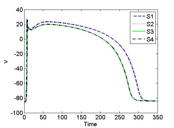
(a)

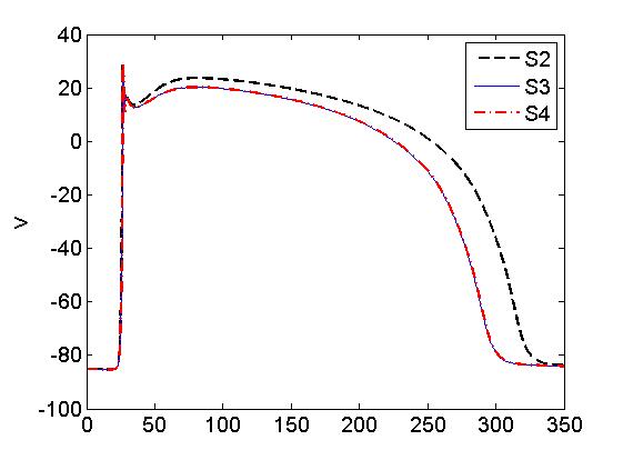
(b)

(c)

(d)

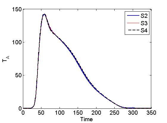
(e)

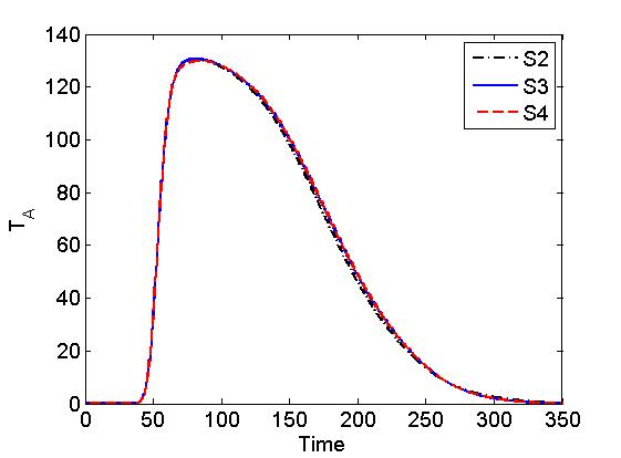
(f)

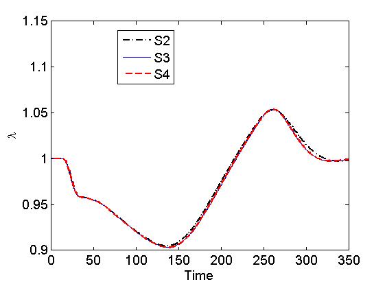
(g)

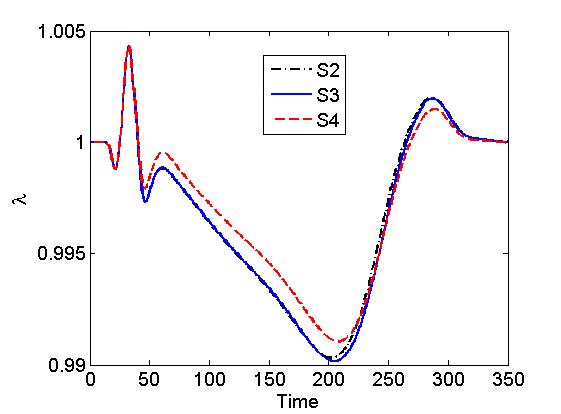
(h)

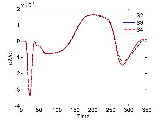
(i)

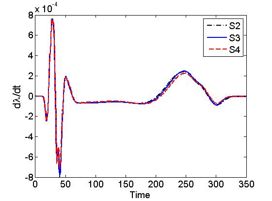
(j)

Figure 2: : $v$ (a), $[Ca^{+2}]_{i}$ (b), $T_{A}$ (c), $\lambda$ (d), $\frac{d\lambda}{dt}(e)$ for the cases, without MEF, without $I_{sac}$, with $I_{sac}$ and with $I_{sac}+$ CONV at M1(column1) and M2(column2).

5.2 (Case 2) Cardiac tissue with ischemic subregion

We consider the cardiac tissue of size $[0,1]^{2}$ with ischemic subregion as $[0.1563,0.25]^{2}$. The ischemic parameters $[K^{+}]_{o}$ and $f_{ATP}$ are varied in the subregion only. The impact of the change for these parameter values are analyzed on the ischemic region and on the healthy neighborhood of the ischemic region. In this case, we will examine the effect at points $M1(0.1875,0.1875)$ and $M2(0.5,0.5)$. $M1$ lies inside the ischemic zone of the cardiac tissue while $M2$ lies in the healthy neighborhood of this ischemic region (see Fig. (3)). Now, we will examine the electrophysiological and the mechanical properties of the cardiac tissue via action potential $(v)$, intracellular calcium concentration $[Ca^{+2}]_{i}$, active tension $T_{A}$, stretch along fiber $(\lambda)$ and stretch rate $(\frac{d\lambda}{dt})$ at these two points.

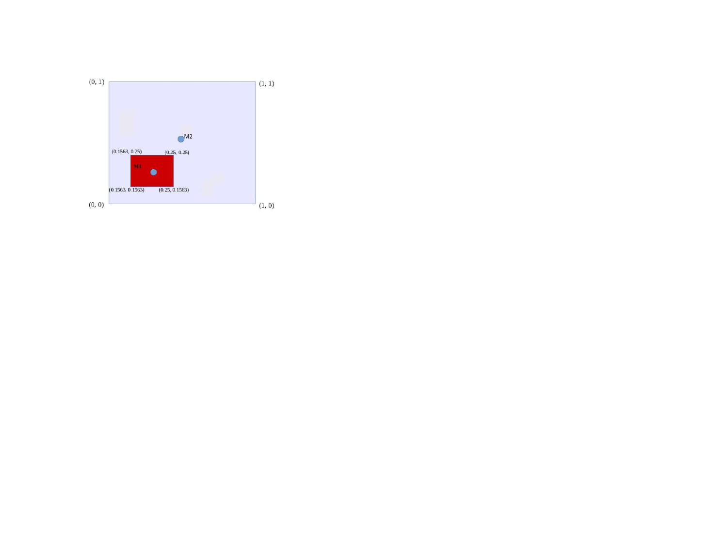
Figure 3: : Cardiac tissue with one ischemic subregion, $M1$ is the point inside the ischemic subregion and $M2$ is outside the ischemic subregion.

5.2.1 (a) Hyperkalemia (Effect of ischemia when only $[K^{+}]_{o}$ varies)

$[K^{+}]_{o}$ is taken in the range $5.4-20mM$ [SR97]. $[K^{+}]_{o}=5.4mM$ is considered as the normal value. In Fig. (4) and (5), action potential $(v)$, intracellular calcium concentration ($[Ca^{+2}]_{i}$), active tension $(T)$, stretch along the fiber $(\lambda)$ and stretch rate $(\frac{d\lambda}{dt})$, at the points $M1$ and $M2$ corresponding to S2, S3 and S4 for different values of $[K^{+}]_{o}$ is drawn. In Fig. (4), effect of Hyperkalemia at the point $M1$ in the ischemic region corresponding to S2, S3 and S4 can be easily visualized. With the increase in the strength of Hyperkalemia, resting potential (RP) increasingly reaches to the higher level of potential values than that of the normal RP value. RP corresponding to S2, S3 and S4 for $[K^{+}]_{o}=20mM$ turns out to be -50mV while the RP for the normal value of $[K^{+}]_{o}$ is -85mV. Thus, there is approximately $40\%$ variation in the RP when Hyperkalemia strength increases up to 20mM. For S2, the ischemic cell repolarize faster than that of the normal cell and hence the APD also reduces with the increase in the Hyperkalemia strength also the cell gets activated earlier as $[K^{+}]_{o}$ reaches to 20mM. This faster repolarization and reduction in APD at M1 is more evident with the addition of the ionic current generated by the stretch activated channels i.e. $(I_{sac})$. While the addition of convective term (i.e. S4) shows negligible change in AP. Changes in the values of APD at $M1$ is given as follows:

	S2	S3	S4
APD (at M1 when $[K^{+}]_{o}=20$mM)	272	265	264

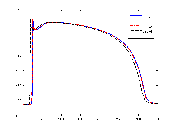
(a)

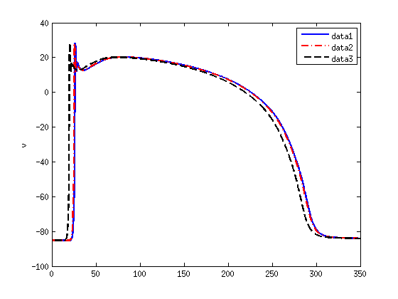
(b)

(c)

(d)

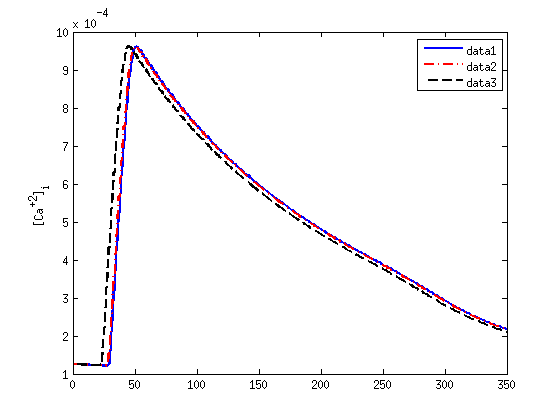
(e)

(f)

(g)

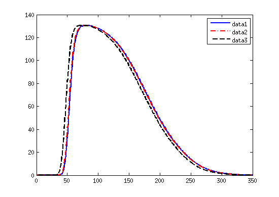
(h)

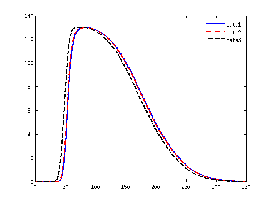
(i)

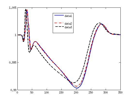
(j)

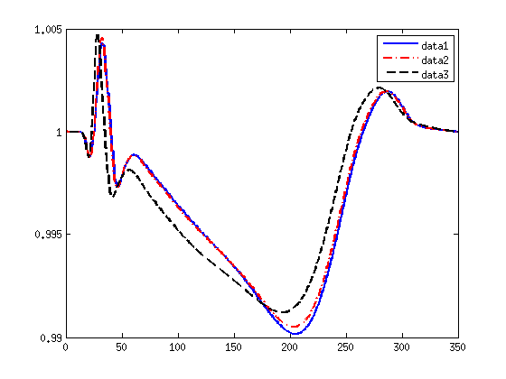
(k)

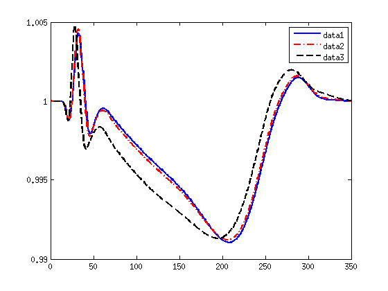
(l)

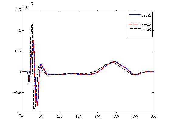
(m)

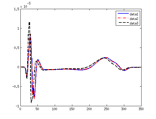
(n)

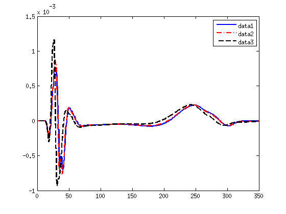
(o)

Figure 5: : $v$ (first row), $[Ca^{+2}]_{i}$ (second row), $T_{A}$ (third row), $\lambda$ (fourth row), $\frac{d\lambda}{dt}$ (fifth row) for the cases without $I_{sac}$ (first column), with $I_{sac}$ (second column) and with $I_{sac}+$ CONV (fourth column) at M2, for different values of $[K^{+}]_{o}$, data1 ($[K^{+}]_{o}=5.4$), data2 ($[K^{+}]_{o}=12$, data3 ($[K^{+}]_{o}=20$).)

From Fig. (5), we can see that at M2 there are small changes in all the phases of the action potential for all the cases S2, S3, and, S4, when $[K^{+}]_{o}$ reaches to 20mM. Early depolarization, faster repolarization is visible. With the addition of $(I_{sac})$ nearby healthy cell M2 goes faster to the resting state while the addition of convective term shows negligible effect.

From Fig. (4(d))- (4(f))and (5(d))-(5(f)), at M1 and M2, changes in the waveform of the concentration of the intracellular calcium ions $[Ca^{+2}]_{i}$ for the cases S2, S3, and S4 are negligible when $[K^{+}]_{o}\leq 12mM$. Changes in the mechanical waveform of $[Ca^{+2}]_{i}$ are visible when $[K^{+}]_{o}$ reaches 20mM and this change in $[Ca^{+2}]_{i}$ waveform leads to change in contraction force and hence contractility of the cardiac tissue. It is to be noticed that at $M1$ and $M2$ the effect in the waveform of $T_{A}$ for the cases S2, S3, and S4 is negligible when $[K^{+}]_{o}\leq 12mM$ and the effect in the change in mechanical waveform of $T_{A}$ is visible when $[K^{+}]_{o}$ reaches to 20mM. It is also clearly visible that the influence of Hyperkalemia on the stretch along fiber $\lambda$ and stretch rate, $\frac{d\lambda}{dt}$ i.e. the change in the waveform of $\lambda$ and hence $\frac{d\lambda}{dt}$ is negligible at M1 corresponding to S2, S3 and S4. The change in the waveform of $\lambda$ and hence $\frac{d\lambda}{dt}$ is more at the point M2 i.e. stretch along the fiber and stretch rate is more with the increase in Hyperkalemia strength. There is more than 3% change in the length of the myocytes relative to the resting length at point M2.

AT, RT and APD contours for S2, S3 and S4 with $[K^{+}]_{o}=20mM$ is presented in Fig. (6)- (8). From Fig. (6), it is visualized form the isochrone lines that the addition of $I_{sac}$ does not affect the AT pattern. Also, increasing the level of Hyperkalemia leads to a visible hastening in the activation of human cardiac cells. An elliptic area is clearly visible which activated earlier than the surrounding one. This indicates that ischemic region generate a new wave.

Fig. (7) and (8) indicates that due to the addition of $I_{sac}$ cardiac cells slightly repolarize faster and hence reduces APD. Also the cardiac cells near to the ischemic region repolarize faster or RT of the ischemic cells or neighboring to the ischemic cells reduces and hence these cells go to the resting state earlier and this tendency increases as the Hyperkalemia gets severe.

In Fig. (9) and (10), we presented the action potential contours in deformation of the cardiac tissue with the increase in the strength of Hyperkalemia, for S2 and S3, respectively. The change in the deformation of cardiac domain with increasing the Hyperkalemic strength is clearly visible.

Next, the effect of increase in the size of the ischemic region from $[0.1563,0.25]^{2}$ to $[0.0938,0.3125]^{2}$ on action potential, intracellular calcium ions $[Ca^{+2}]_{i}$, active tension $T_{A}$, stretch along the fiber $\lambda$ and stretch rate, $\frac{d\lambda}{dt}$ are presented in Fig. (11) for the case $[K^{+}]_{o}=20$mM. Clearly the spread of severe Hyperkalemic ischemic zone further raises already increased resting potential levels, at $M1$, from -50mV to -45mV respectively. Also the growth in ischemic size leads to faster repolarization with a reduced APD. There is almost $9\%$ further drop in APD is noticed with a factor of five times increase in the ischemic subregion size. From the action potential plot corresponding to point $M2$, it is visible that there is almost $5\%$ drop in APD for this neighboring healthy cell. Thus, it is amply clear that in the proximity of ischemic subregion the CEA in terms of action potential and hence the ECG of healthy cardiac tissue is affected with the severity of Hyperkalemia. This effect in the ischemic and healthy cells will increase with the spread of ischemic region.

It is also noticed that there is variation in the waveform of $[Ca^{+2}]_{i}$ at M1 while it is going to rest, but at M2 the waveform changes during all the phases. The variation in the stretch along the fiber and the stretch rate is more in the neighboring region point M2 with the expansion of the ischemic region while the change at the point M1 inside the ischemic region is negligible. In short, expanding the ischemic region size affect the mechanical properties of the neighboring healthy cells more intensely.

Hence, it could be concluded that addition of $I_{sac}$ leads to ECG change and mechanical contraction as it reduces the APD and affects the contractility and the length of length of myocytes of healthy and ischemic parts of the human cardiac tissue. It is also observed that the severity of Hyperkalemia leads to reduction in APD, elevation in resting potential, affects the contractile force and contractility and the stretch activated channels, hence affects the QRS complex and QT interval of ECG and the mechanical contraction or can say the electro-mechanical activity of healthy and ischemic regions of human cardiac tissue. All these effects on the electro-mechanical activity of a human heart gets more intense as the ischemic regions expands or more cardiac cells becomes ischemic.

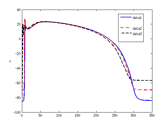
(a)

(b)

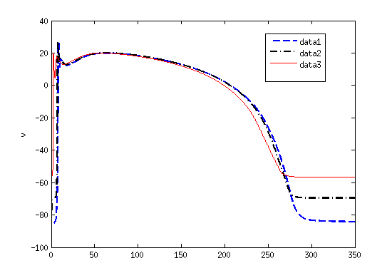
(c)

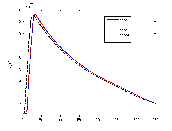
(d)

(e)

(f)

(g)

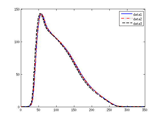
(h)

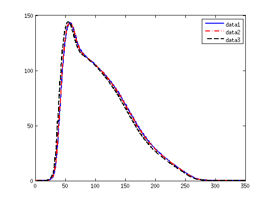
(i)

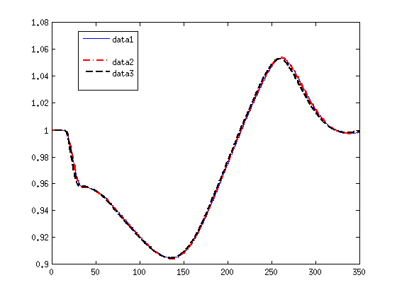
(j)

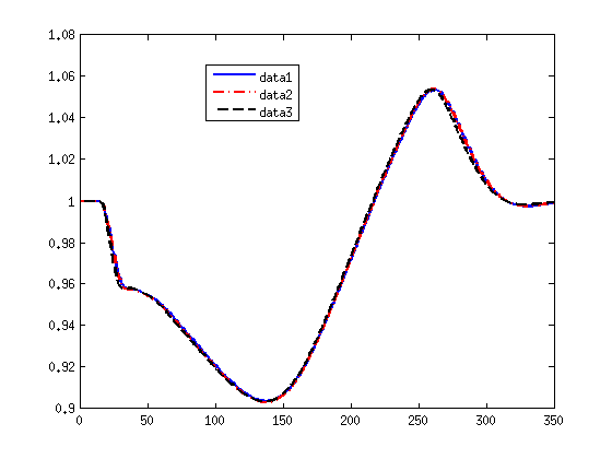
(k)

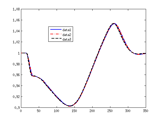
(l)

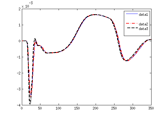
(m)

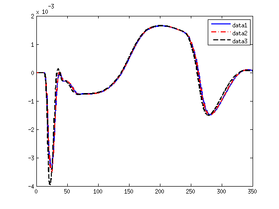
(n)

(o)

Figure 4: : $v$ (first row), $[Ca^{+2}]_{i}$ (second row), $T_{A}$ (third row), $\lambda$ (fourth row), $\frac{d\lambda}{dt}$ (fifth row) for the cases without $I_{sac}$ (first column), with $I_{sac}$ (second column) and with $I_{sac}+$ CONV (fourth column) at M1, for different values of $[K^{+}]_{o}$, data1 ($[K^{+}]_{o}=5.4$), data2 ($[K^{+}]_{o}=12$), data3 ($[K^{+}]_{o}=20$)).

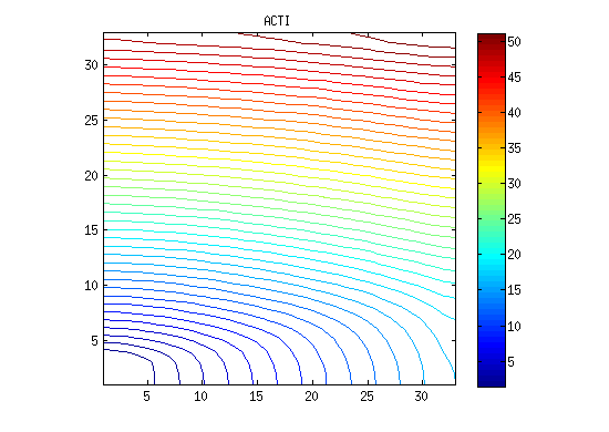
(a)

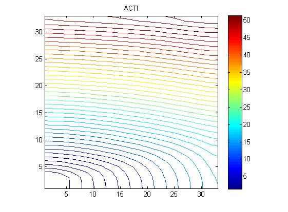
(b)

(c)

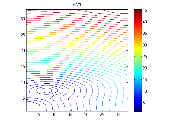
(d)

(e)

(f)

Figure 6: : AT for the cases without $I_{sac}$ (first column), with $I_{sac}$ (second column) and with $I_{sac}+$ CONV (third column) for $[K^{+}]_{o}=5.4$mM (first row) and $[K^{+}]_{o}=20$mM (second row).

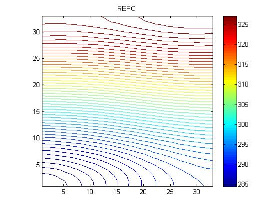
(a)

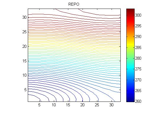
(b)

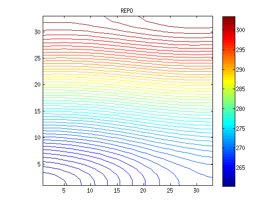
(c)

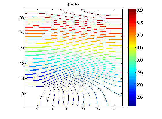
(d)

(e)

(f)

Figure 7: : RT for the cases without $I_{sac}$ (first column), with $I_{sac}$ (second column) and with $I_{sac}+$ CONV (third column) for $[K^{+}]_{o}=5.4$mM (first row) and $[K^{+}]_{o}=20$mM (second row).

(a)

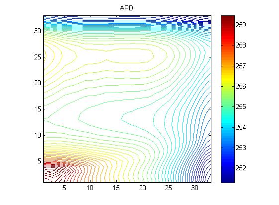
(b)

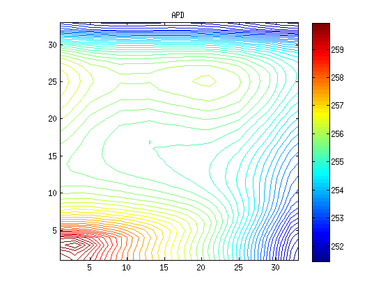
(c)

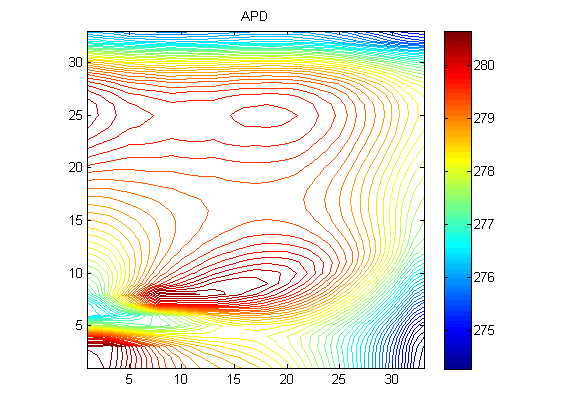
(d)

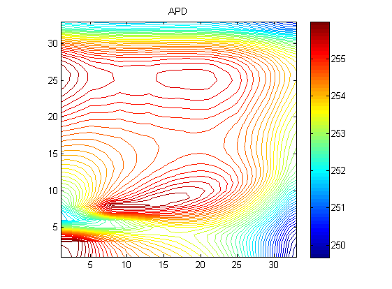
(e)

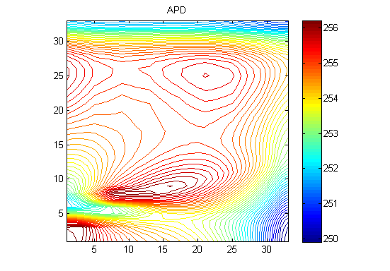
(f)

Figure 8: : APD for the cases without $I_{sac}$ (first column), with $I_{sac}$ (second column) and with $I_{sac}+$ CONV (third column) for $[K^{+}]_{o}=5.4$mM (first row) and $[K^{+}]_{o}=20$mM (second row).

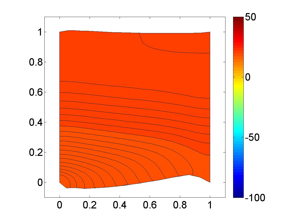
(a)

(b)

(c)

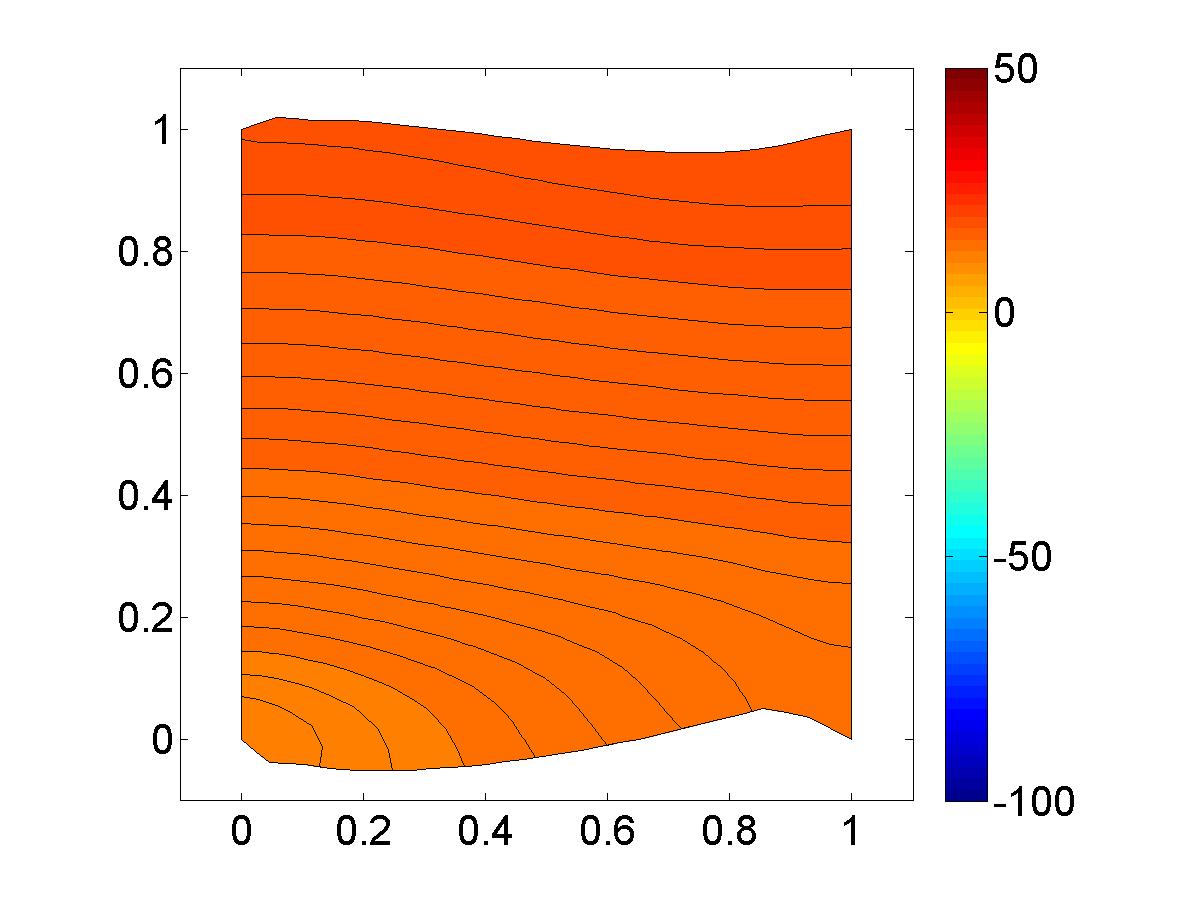
(d)

(e)

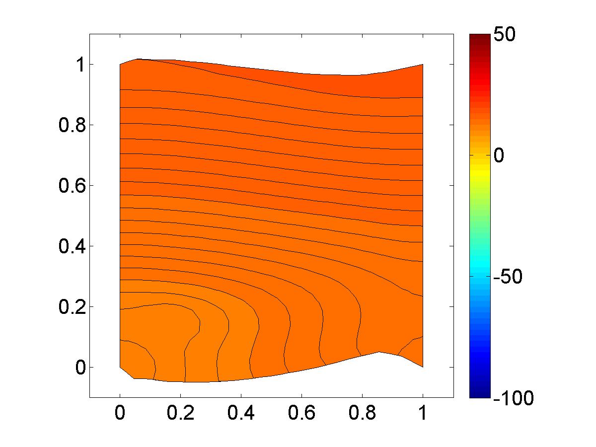
(f)

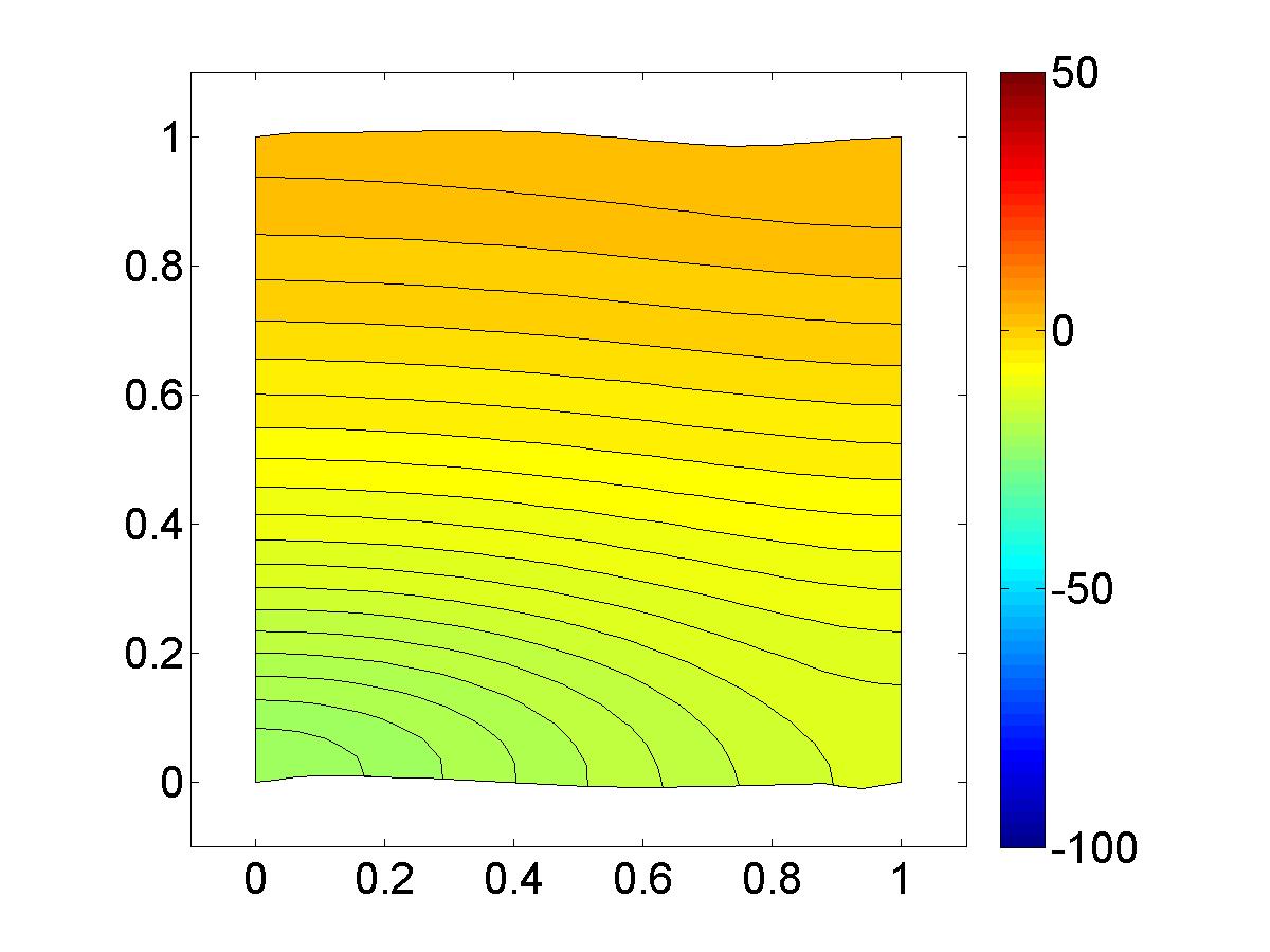
(g)

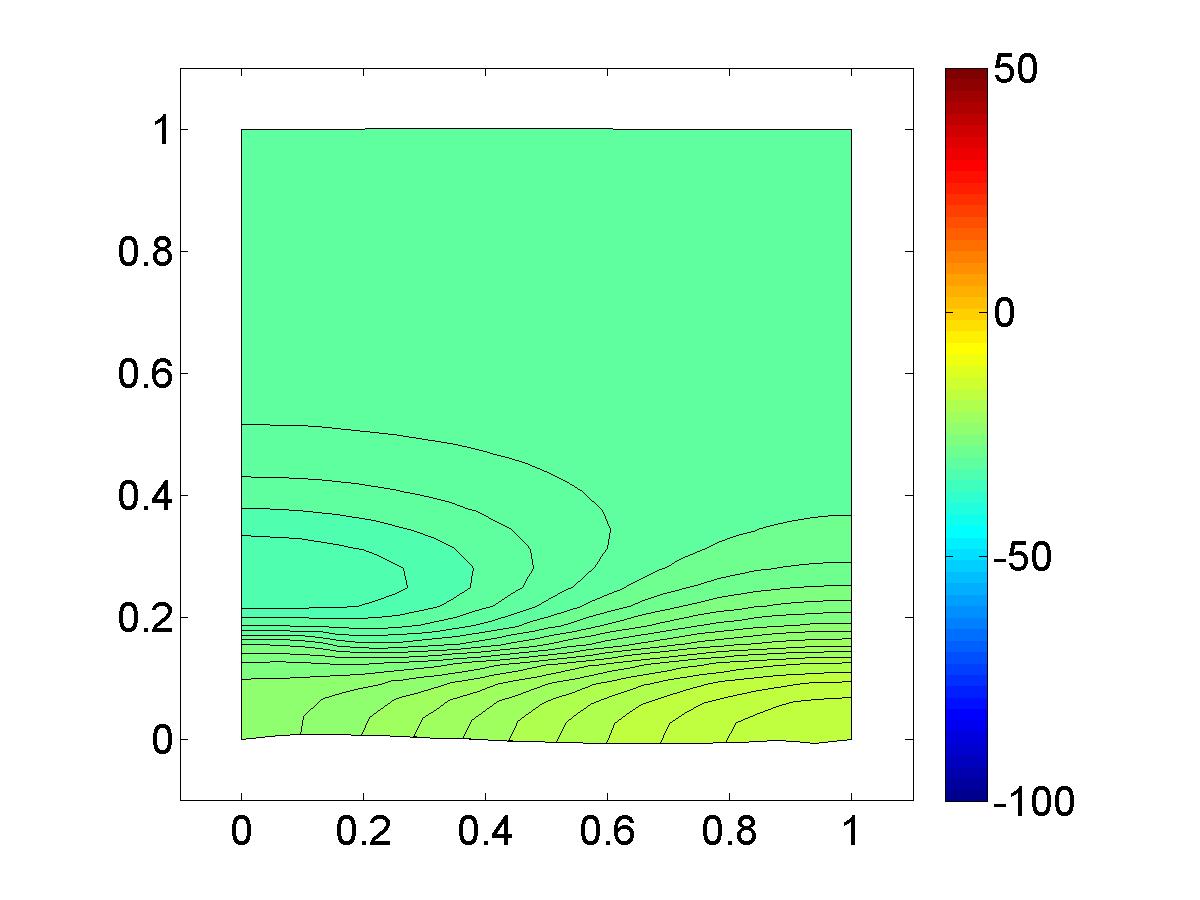
(h)

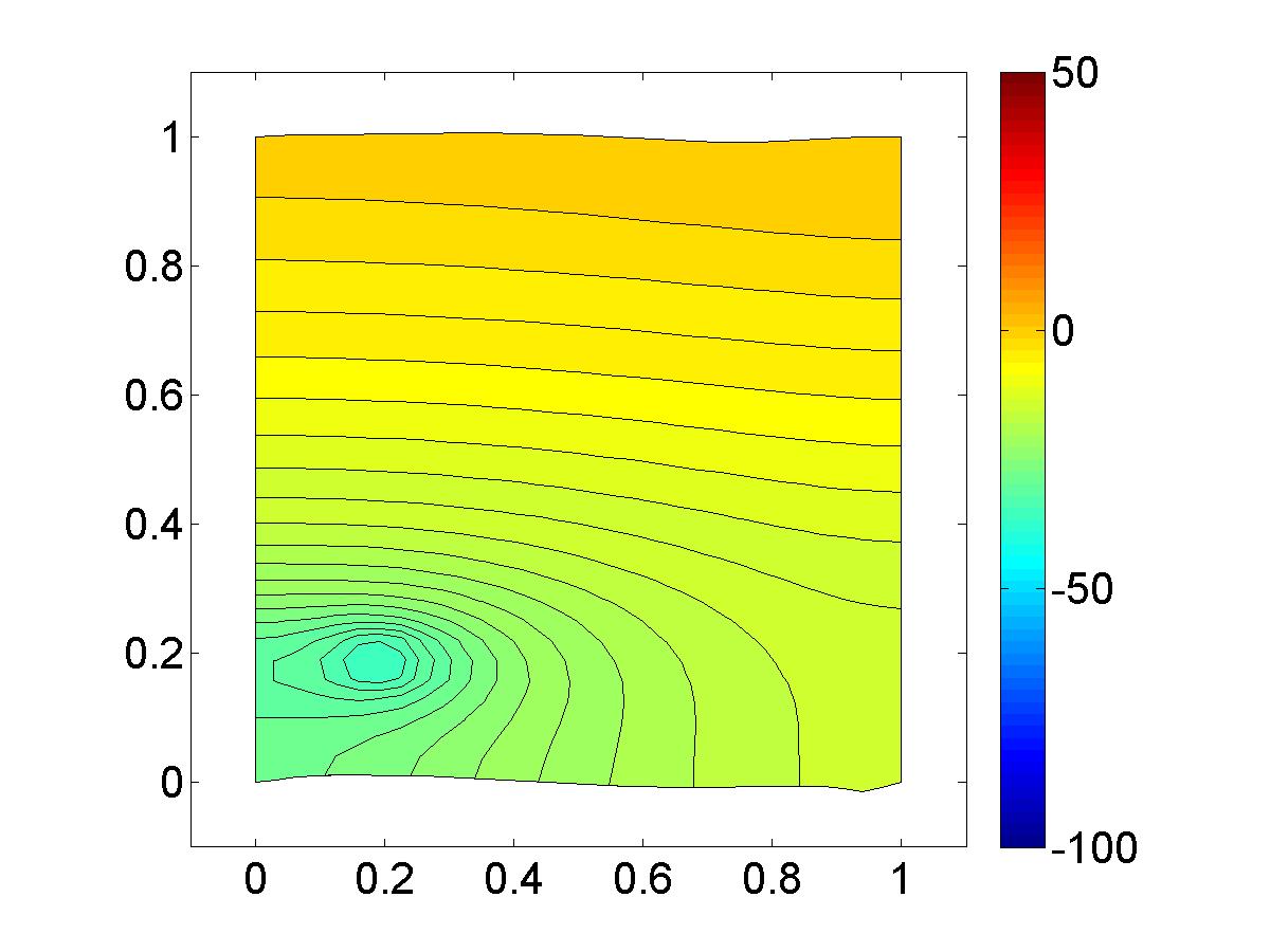
(i)

Figure 9: : Action potential contours in a deforming domain for the cases without $I_{sac}$ for different values of $[K^{+}]_{o}$ = 5.4 mM (first column), $[K^{+}]_{o}$=12 mM (second column), $[K^{+}]_{o}$ = 20 mM (third column), at time t=90 (first row), t=150 (second row), t=240 (third row).

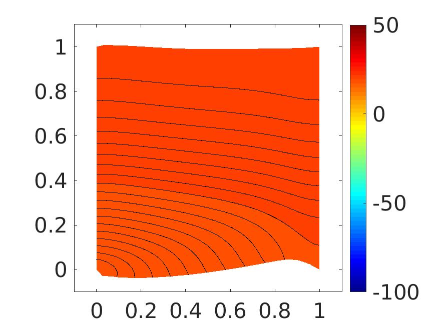
(a)

(b)

(c)

(d)

(e)

(f)

(g)

(h)

(i)

Figure 10: : Action potential contours in a deforming domain for the cases with $I_{sac}$ for different values of $[K^{+}]_{o}$ =5.4 (first column), $[K^{+}]_{o}$=12 (second column), $[K^{+}]_{o}$ = 20 (third column), at time t=90 (first row), t=150 (second row), t=240 (third row).

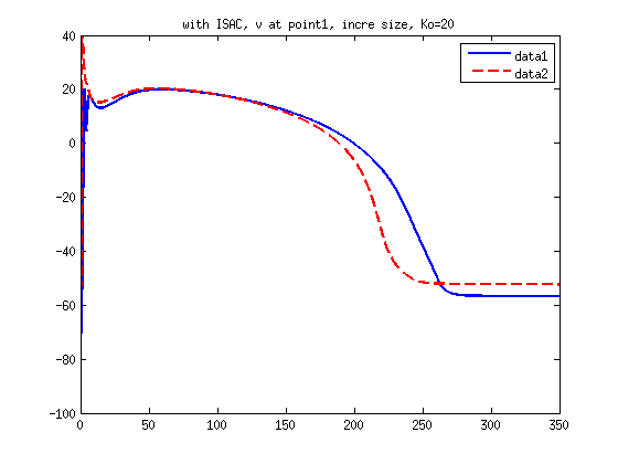
(a)

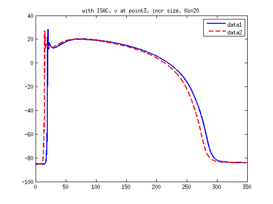
(b)

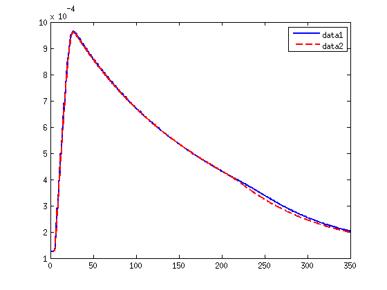
(c)

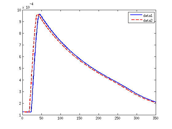
(d)

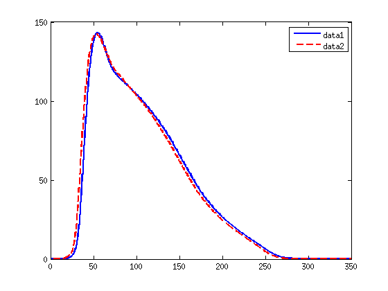
(e)

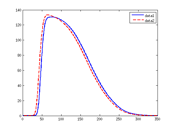
(f)

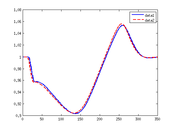
(g)

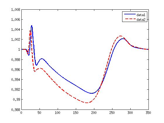
(h)

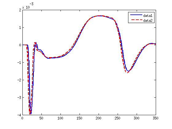
(i)

(j)

Figure 11: : $v$(first row), $[Ca^{+2}]_{i}$(second row), $T_{A}$(third row), $\lambda$ (fourth row) and $\frac{d\lambda}{dt}$ (fifth row), at M1(first column), M2 (second column), for the case with $I_{sac}$ (second column) for $[K^{+}]_{o}=20$, with two different sizes of ischemic regions, data1 ($[0.1563,0.25]^{2}$), data2 ($[0.0938,0.3125]^{2}$).

Note: As it is concluded that the addition of $I_{sac}$ plays an important role in the electro-mechanical activity of a human cardiac tissue. So, next results will be with $I_{sac}$ case only.

5.2.2 (a) Hypoxia (Effect of ischemia when only $f_{ATP}$ varies)

$f_{ATP}$ is taken in the range $0.1-0.5\%$. Influence of the $f_{ATP}$ values (oxygen level) on the action potential and the mechanical parameters $[Ca^{+2}]_{i}$, active tension $(T_{A})$, stretch along the fiber $(\lambda_{l})$ and stretch rate $(\frac{d\lambda_{l}}{dt})$ at the two points $M1$ and $M2$ (described above) of the cardiac tissue are estimated and presented in Fig. (12). From Fig. (12(a)), it can be seen that as the oxygen level in the ischemic region of the cardiac tissue decreases (or $f_{ATP}$ value increased), delay in the closing of L-type $Ca^{+2}$ channels is noticed, and further rapid close of the $K^{+}$ channels takes place, therefore the plateau phase and then the repolarization phase of the cardiac action potential get affected. Therefore, APD also reduces with the increase in the strength of Hypoxia. While from the Fig. (12(b)), it can be seen that influence of the increase in $f_{ATP}$ values is negligible on the neighborhood point M2 on the non-ischemic region of cardiac tissue.

Further from figures (12(c)) - (12(j)), it is visulaized that there is negligible change in the waveform of the mechanical parameters, intracellular calcium concentration ($[Ca^{+2}]_{i}$), active tension $(T_{A})$, stretch along the fiber $(\lambda_{l})$ and stretch rate $(\frac{d\lambda_{l}}{dt})$ at the points $M1$ and $M2$.

From Fig. (13(a))-(13(g)), it is clear that the activation time remain unaffected by $f_{ATP}$ and hence the isochrones of AT corresponding to these cases turn out to be same in the entire domain including those in ischemic region. The front near the ischemic region is quasi elliptic and becomes flat after that.

RT isochrones show that as we increase the $f_{ATP}$ values in the ischemic region i.e. as the oxygen level in the ischemic region of the cardiac tissue decreases, the cardiac cells in the ischemic region repolarize earlier i.e. the repolarization time of ischemic cell decreases with the increase in $f_{ATP}$ values while the repolarization time for the non-ischemic cardiac cells remains same. The loss of quasi-ellipticity and the folding of repolarization time isochrones especially in the ischemic subregion depict an accelerated repolarization wave propagation in the human cardiac tissue. The isochrone lines for APD shows that APD in the ischemic region reduces as we are increasing $f_{ATP}$ values.

In Fig. (14(a))-(14(i)), we presented the action potential contours in deforming cardiac tissue with the increase in the strength of Hypoxia. We can visualize the change in the deformation of cardiac domain with the increasing Hypoxic strength. Thus, change in oxygen level affects the contraction and expansion of ventricle of human heart.

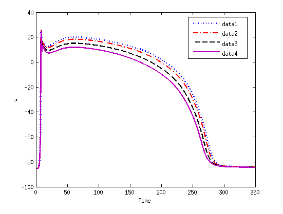
(a)

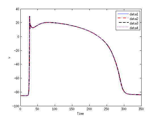
(b)

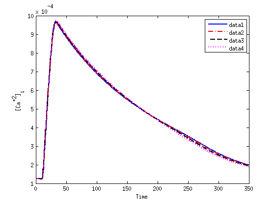
(c)

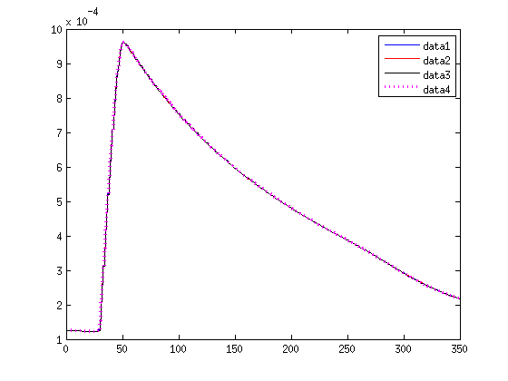
(d)

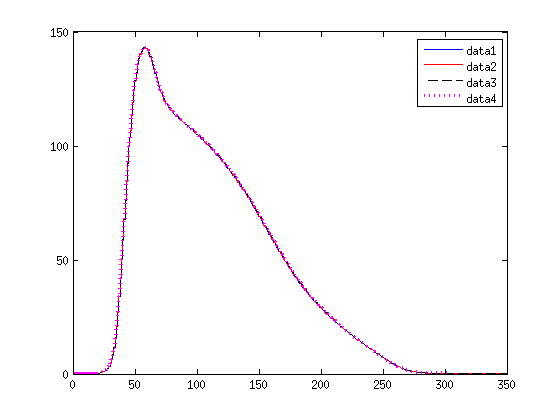
(e)

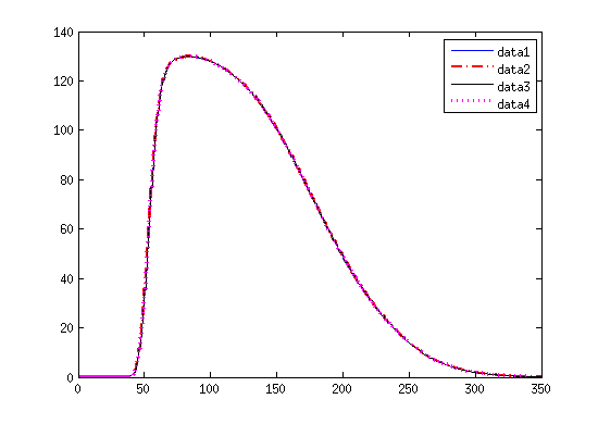
(f)

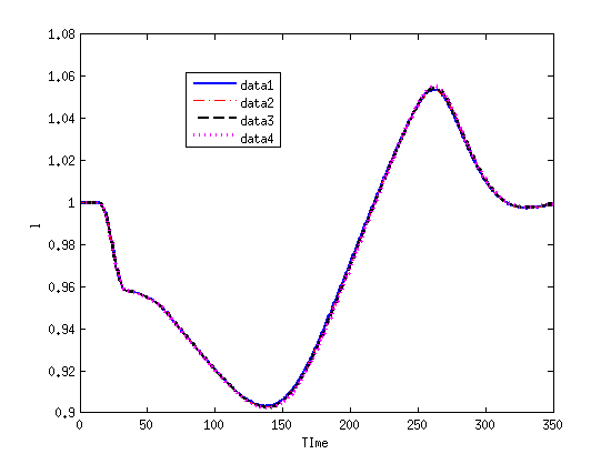
(g)

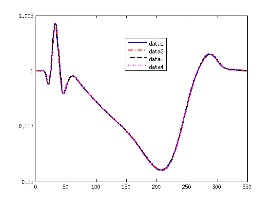
(h)

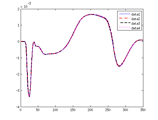
(i)

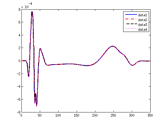
(j)

Figure 12: :$v$(first row), $[Ca^{+2}]_{i}$(second row), $T_{A}$(third row), $\lambda$ (fourth row) and $\frac{d\lambda}{dt}$ (fifth row), at M1(first column), M2 (second column), for different values of $f_{ATP}$. data1 ($f_{ATP}=0$), data2 ($f_{ATP}=0.1\%$), data3 ($f_{ATP}=0.3\%$), data4 ($f_{ATP}=0.5\%$).

(a)

(b)

(c)

(d)

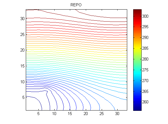
(e)

(f)

(g)

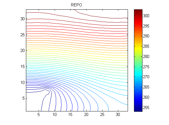
(h)

(i)

Figure 13: :AT (first column), RT (second column), APD (third column) for different values of $f_{ATP}=0$(first row), $f_{ATP}=0.1\%$(second row), $f_{ATP}=0.3\%$(third row), $f_{ATP}=0.5\%$(fourth row).

(a)

(b)

(c)

(d)

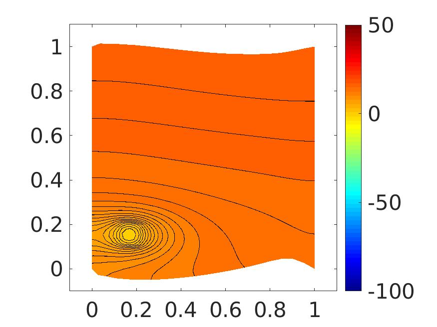
(e)

(f)

(g)

(h)

(i)

Figure 14: :AP contours in a deforming domain for different values of $f_{APT}$ =0 (first row), $f_{APT}=0.3\%$ (second row), $f_{APT}=0.5\%$ (third row), at time t=90 (first column), t=150 (seconf column), t=240 (third column).

Next, as we increase the size of the ischemic region from $[0.1563,0.25]^{2}$ to $[0.0938,0.3125]^{2}$, action potential at the points M1 and M2 get influenced as shown in Fig (15). From the Fig (15(a)), we can conclude that, at $M_{1}$ (ischemic region point), with the increase in the size of the ischemic region there is further delay in the closing of L-type calcium channels. Thus, a delay in plateau phase and then early repolarization of the action potential takes place. APD also reduces with increase in the size of the ischemic region. From the action potential plot corresponding to point $M_{2}$ in Fig. (15(b)), a delay in plateau phase and early repolarization of the action potential and reduction in the APD of these neighboring cells is also clearly visible. At $M1$ there is $11\%$ drop in APD with a factor of five times increase in the ischemic region size. Depending on the distance of the neighboring points from the ischemic region, more than $5\%$ drop in APD with a factor of five times increase in the ischemic region size is noticed.

Now, from Fig. (15(c)) - (15(j)), it is visible that increasing the size of the ischemic region also considerably affects the waveforms of the mechanical parameters $[Ca^{+2}]_{i}$, $T_{A}$, $\lambda$ and $\frac{d\lambda}{dt}$ corresponding to the point M1 than those of the point M2. From the figures (15(g)) and (15(h)), it can be noticed that an increase in the size of the ischemic region by a factor of five leads to additional shortening of fiber length during systolic contraction and an enhanced stretch in the fibers post systolic contraction. At $M1$ $3-4\%$ change in the length of the myocytes relative to the resting length is noticed and at $M_{2}$ only a $1-2\%$ change in the length of the myocytes relative to the resting length is noticed. Therefore, the stretch rate $\frac{d\lambda}{dt}$ also changes at the points $M_{1}$ and $M_{2}$. There is approximately $45\%$ variation in the stretch rate $\frac{d\lambda}{dt}$ at $M1$ and approximately $5-25\%$ variation in the neighboring points is detected.

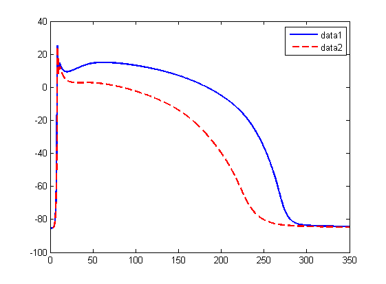
(a)

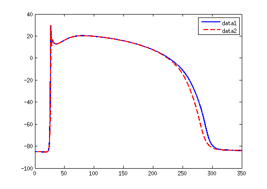
(b)

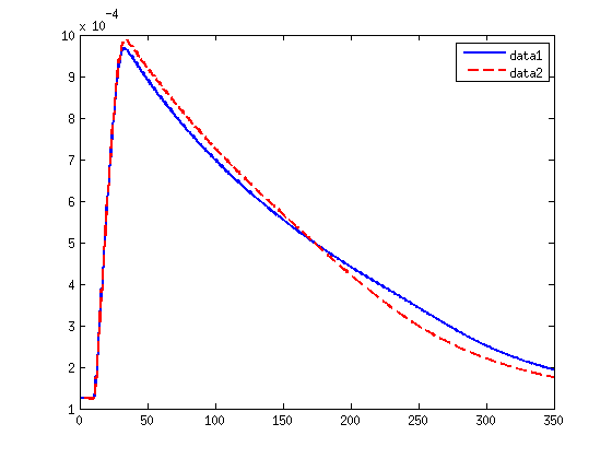
(c)

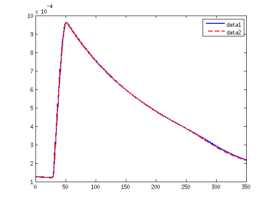
(d)

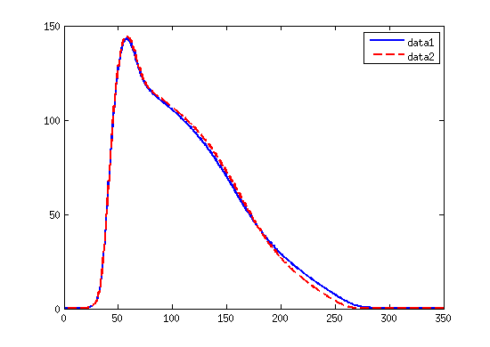
(e)

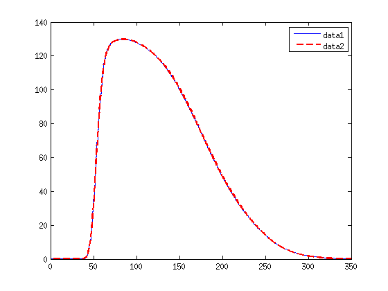
(f)

(g)

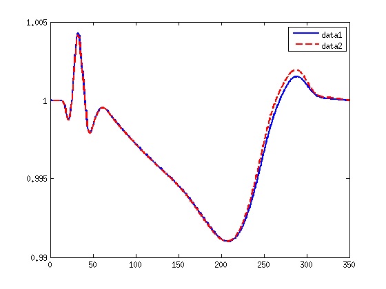
(h)

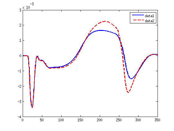
(i)

(j)

Figure 15: :$v$(first row), $[Ca^{+2}]_{i}$(second row), $T_{A}$(third row), $\lambda$ (fourth row) and $\frac{d\lambda}{dt}$ (fifth row), at M1(first column), M2 (second column), for the case with $I_{sac}$ (second column) for $f_{ATP}=0.3\%$, with two different sizes of ischemic regions, data1 ($[0.1563,0.25]^{2}$), data2 ($[0.0938,0.3125]^{2}$).

Thus, the cardiac electro-mechanical activity mathematically generated by PDE-ODE system leads to tracing of ionic channel dynamics, intracellular calcium ion abnormalities including the tissue structural influences. It may be noted that the ionic channels corresponding to each cardiac cell adds to the generation of cardiac action potential and also forms the basis for calcium induction, calcium release and cardiac mechanical contraction. The change in the action potential phase and hence in ECG pattern affects both the electrical and mechanical function of heart. These numerical results help in tracing the affected action potential phase, leading to a disturbance in ECG pattern. It also helps in identification of corresponding affected ionic channel dynamics. Thus, the current analysis can provide a useful guideline for the treatment of Hyperkalemia and Hypoxia.

Thus, the heart failure due to the cardiac disease from the abnormal functioning of the coupled electrical and mechanical activity can be traced through the virtual reconstruction of ionic channels and intracellular calcium ion abnormalities with cardiac structural reconstruction through the proposed numerical modeling. The ionic channels corresponding to each cardiac cell adds to the generation of cardiac action potential and also forms the basis for calcium induction, calcium release and cardiac mechanical contraction. The change in the action potential phase and hence in ECG pattern affects both the electrical and mechanical function of heart.

6 Conclusion

Local ischemia in the deformed human cardiac tissue is modeled by varying the ischemic parameters value in the ischemic subregion of the cardiac tissue domain. Two types of ischemic effects, namely, Hyperkalemia and Hypoxia, are considered in this work. Monodomain model in a deforming domain is taken with the TT06 human cell level model. The coupled electro-mechanical PDEs-ODEs non-linear system of equations are solved numerically using linear finite elements in space and backward Euler finite difference scheme in time. We examine the cardiac electrical and mechanical activity in terms of the action potential ($v$) and intracellular calcium ion concentration $[Ca^{+2}]_{i}$, active tension, ($T_{A}$), stretch ($\lambda$), stretch rate ($\frac{d\lambda}{dt}$), in several cases for local ischemia. We investigated the effect of varying strength of Hyperkalemia and Hypoxia in the ischemic subregion of cardiac tissue, on the electrical and mechanical activity of healthy and ischemic zones in the cardiac muscle. We also investigated the impact of increasing the size of the ischemic region on the electrical and mechanical parameters of neighboring cells.

(a) With the severity of Hyperkalemia the concentration of extracellular potassium ions increase leading to, (i) Fall in availability of sodium channels and a decrease in inward sodium current, (ii) AP comes to a resting state significantly prior to reaching the normal resting potential level, and, (iii) Increased potassium conductance leading to shortening of RT in turn shortens QT interval is noticed.

These changes in cellular ionic dynamics not only further alters the AT, RP, RT and APD of affected cells with the spread of Hyperkalemic region but also increasingly alters the AP of healthy cells in its vicinity. Also, this spread of Hyperkalemic region alters the waveform of the mechanical parameters $[Ca^{+2}]_{i},T_{A},\lambda$ ,$\frac{d\lambda}{dt}$ of the ischemic and the neighboring healthy cells.

Thus, the severity of Hyperkalemia leads to reduction in APD, elevation in resting potential, affects the contractile force and contractility and the stretch activated channels, hence affects the QRS complex and QT interval of ECG and the mechanical contraction or can say the electro-mechanical activity of healthy and ischemic regions of human cardiac tissue. All these effects on the electro-mechanical activity of a human heart gets more intense as the ischemic regions expands or more cardiac cells becomes ischemic.

(b) Severity of Hypoxic ischemia, with a reduction in intracellular ATP concentration, affect both influx of calcium ions and efflux of potassium ions and alters the normal functioning of calcium channels and balanced potassium channels. The increase in intracellular $Ca^{+2}$ levels completely disturbs the Phase1, Phase2 and Phase 3 of AP. As the Hypoxically affected region increases, the Plateau phase, repolarization phase and the APD corresponding to the AP of healthy cells in its vicinity are affected and the ionic dynamics of Hypoxically already degenerated cells get further disturbed. It is also visible that increasing the size of the ischemic region by a factor of five considerably affects the waveforms of the mechanical parameters $[Ca^{+2}]_{i}$, $T_{A}$, $\lambda$ and $\frac{d\lambda}{dt}$. There is approximately $45\%$ variation in the stretch rate $\frac{d\lambda}{dt}$ at $M1$ and approximately $5-25\%$ variation in the neighboring points is detected.

Thus, the change in the action potential phase and hence in ECG pattern affects both the electrical and mechanical function of heart. These numerical results help in tracing the affected action potential phase, leading to a disturbance in ECG pattern. It also helps in identification of corresponding affected ionic channel dynamics. Thus, the current analysis can provide a useful guideline for the treatment of Hyperkalemia and Hypoxia.

Financial disclosure

We would like to thank the DST for support through Inspire Fellowship, ID no. is IF130906. We would also like to thanks the ICTP-INdAM.

CONFLICTS OF INTEREST

The authors declare no potential conflict of interests.

References

- [AANQ11] Davide Ambrosi, Gianni Arioli, Fabio Nobile, and Alfio Quarteroni. Electromechanical coupling in cardiac dynamics: the active strain approach. SIAM Journal on Applied Mathematics, 71(2):605–621, 2011.
- [AB14] Tareg M Alsoudani and Ian David Lockhart Bogle. From discretization to regularization of composite discontinuous functions. Computers & Chemical Engineering, 62:139–160, 2014.
- [ABQRB15] Boris Andreianov, Mostafa Bendahmane, Alfio Quarteroni, and Ricardo Ruiz-Baier. Solvability analysis and numerical approximation of linearized cardiac electromechanics. Mathematical Models and Methods in Applied Sciences, 25(05):959–993, 2015.
- [AHZ13a] Ismail Adeniran, Jules C Hancox, and Henggui Zhang. Effect of cardiac ventricular mechanical contraction on the characteristics of the ecg: a simulation study. Journal of Biomedical Science and Engineering, 6(12):47, 2013.
- [AHZ13b] Ismail Adeniran, Jules C Hancox, and Henggui Zhang. Effect of cardiac ventricular mechanical contraction on the characteristics of the ecg: a simulation study. Journal of Biomedical Science and Engineering, 6(12):47, 2013.
- [AP96] Rubin R Aliev and Alexander V Panfilov. A simple two-variable model of cardiac excitation. Chaos, Solitons & Fractals, 7(3):293–301, 1996.
- [BMST18] Mostafa Bendahmane, Fatima Mroue, Mazen Saad, and Raafat Talhouk. Mathematical analysis of cardiac electromechanics with physiological ionic model. 2018.
- [Car99] Edward Carmeliet. Cardiac ionic currents and acute ischemia: from channels to arrhythmias. Physiological reviews, 79(3):917–1017, 1999.
- [CBP+14a] Valentina Carapella, Rafel Bordas, Pras Pathmanathan, Maelene Lohezic, Jurgen E Schneider, Peter Kohl, Kevin Burrage, and Vicente Grau. Quantitative study of the effect of tissue microstructure on contraction in a computational model of rat left ventricle. PloS one, 9(4):e92792, 2014.
- [CBP+14b] Valentina Carapella, Rafel Bordas, Pras Pathmanathan, Maelene Lohezic, Jurgen E Schneider, Peter Kohl, Kevin Burrage, and Vicente Grau. Quantitative study of the effect of tissue microstructure on contraction in a computational model of rat left ventricle. PloS one, 9(4):e92792, 2014.
- [CFPS07] Piero Colli Franzone, Luca F. Pavarino, and Simone Scacchi. Dynamical effects of myocardial ischemia in anisotropic cardiac models in three dimensions. Math. Models Methods Appl. Sci., 17(12):1965–2008, 2007.
- [CFPS16] Piero Colli Franzone, Luca F Pavarino, and Simone Scacchi. Bioelectrical effects of mechanical feedbacks in a strongly coupled cardiac electro-mechanical model. Mathematical Models and Methods in Applied Sciences, 26(01):27–57, 2016.
- [CHLT13] Jason Constantino, Yuxuan Hu, Albert C Lardo, and Natalia A Trayanova. Mechanistic insight into prolonged electromechanical delay in dyssynchronous heart failure: a computational study. American Journal of Physiology-Heart and Circulatory Physiology, 2013.
- [CHM01] Kevin D Costa, Jeffrey W Holmes, and Andrew D McCulloch. Modelling cardiac mechanical properties in three dimensions. Philosophical transactions of the Royal Society of London. Series A: Mathematical, physical and engineering sciences, 359(1783):1233–1250, 2001.
- [Cor94] Ruben Coronel. Heterogeneity in extracellular potassium concentration during early myocardial ischaemia and reperfusion: implications for arrhythmogenesis. Cardiovascular research, 28(6):770–777, 1994.
- [DGKK13] Hüsnü Dal, Serdar Göktepe, Michael Kaliske, and Ellen Kuhl. A fully implicit finite element method for bidomain models of cardiac electromechanics. Computer methods in applied mechanics and engineering, 253:323–336, 2013.
- [DMZ+16] Sara Dutta, Ana Mincholé, Ernesto Zacur, T Alexander Quinn, Peter Taggart, and Blanca Rodriguez. Early afterdepolarizations promote transmural reentry in ischemic human ventricles with reduced repolarization reserve. Progress in biophysics and molecular biology, 120(1-3):236–248, 2016.
- [DORB+13] BL De Oliveira, BM Rocha, LPS Barra, EM Toledo, J Sundnes, and R Weber dos Santos. Effects of deformation on transmural dispersion of repolarization using in silico models of human left ventricular wedge. International Journal for Numerical Methods in Biomedical Engineering, 29(12):1323–1337, 2013.
- [EPPH13] Thomas SE Eriksson, AJ Prassl, Gernot Plank, and Gerhard A Holzapfel. Influence of myocardial fiber/sheet orientations on left ventricular mechanical contraction. Mathematics and Mechanics of Solids, 18(6):592–606, 2013.
- [FBS+85] JWT Fiolet, A Baartscheer, CA Schumacher, HF Ter Welle, and WJG Krieger. Transmural inhomogeneity of energy metabolism during acute global ischemia in the isolated rat heart: dependence on environmental conditions. Journal of molecular and cellular cardiology, 17(1):87–92, 1985.
- [FKF+91] Tetsushi Furukawa, Shinichi Kimura, Nanako Furukawa, Arthur L Bassett, and Robert J Myerburg. Role of cardiac atp-regulated potassium channels in differential responses of endocardial and epicardial cells to ischemia. Circulation research, 68(6):1693–1702, 1991.
- [GCM95a] Julius M Guccione, Kevin D Costa, and Andrew D McCulloch. Finite element stress analysis of left ventricular mechanics in the beating dog heart. Journal of biomechanics, 28(10):1167–1177, 1995.
- [GCM95b] Julius M Guccione, Kevin D Costa, and Andrew D McCulloch. Finite element stress analysis of left ventricular mechanics in the beating dog heart. Journal of biomechanics, 28(10):1167–1177, 1995.
- [GCRT10] V Gurev, J Constantino, JJ Rice, and NA Trayanova. Distribution of electromechanical delay in the heart: insights from a three-dimensional electromechanical model. Biophysical journal, 99(3):745–754, 2010.
- [GK10a] Serdar Göktepe and Ellen Kuhl. Electromechanics of the heart: a unified approach to the strongly coupled excitation–contraction problem. Computational Mechanics, 45(2-3):227–243, 2010.
- [GK10b] Serdar Göktepe and Ellen Kuhl. Electromechanics of the heart: a unified approach to the strongly coupled excitation–contraction problem. Computational Mechanics, 45(2-3):227–243, 2010.
- [GLC+11] Viatcheslav Gurev, Ted Lee, Jason Constantino, Hermenegild Arevalo, and Natalia A Trayanova. Models of cardiac electromechanics based on individual hearts imaging data. Biomechanics and modeling in mechanobiology, 10(3):295–306, 2011.
- [HMTK98] PJ Hunter, AD McCulloch, and HEDJ Ter Keurs. Modelling the mechanical properties of cardiac muscle. Progress in biophysics and molecular biology, 69(2-3):289–331, 1998.
- [HO09] Gerhard A Holzapfel and Ray W Ogden. Constitutive modelling of passive myocardium: a structurally based framework for material characterization. Philosophical Transactions of the Royal Society A: Mathematical, Physical and Engineering Sciences, 367(1902):3445–3475, 2009.
- [HS97] Hai Hu and Frederick Sachs. Stretch-activated ion channels in the heart. Journal of molecular and cellular cardiology, 29(6):1511–1523, 1997.
- [JGT10] Xiao Jie, Viatcheslav Gurev, and Natalia Trayanova. Mechanisms of mechanically induced spontaneous arrhythmias in acute regional ischemia. Circulation research, 106(1):185–192, 2010.
- [JW89] Michiel J Janse and ANDREW L Wit. Electrophysiological mechanisms of ventricular arrhythmias resulting from myocardial ischemia and infarction. Physiological reviews, 69(4):1049–1169, 1989.
- [KBK+03] RCP Kerckhoffs, PHM Bovendeerd, JCS Kotte, FW Prinzen, K Smits, and T Arts. Homogeneity of cardiac contraction despite physiological asynchrony of depolarization: a model study. Annals of biomedical engineering, 31(5):536–547, 2003.
- [KNP09] RH Keldermann, MP Nash, and AV Panfilov. Modeling cardiac mechano-electrical feedback using reaction-diffusion-mechanics systems. Physica D: Nonlinear Phenomena, 238(11-12):1000–1007, 2009.
- [KOMM10] Roy CP Kerckhoffs, Jeffrey H Omens, Andrew D McCulloch, and Lawrence J Mulligan. Ventricular dilation and electrical dyssynchrony synergistically increase regional mechanical nonuniformity but not mechanical dyssynchrony: a computational model. Circulation: Heart Failure, 3(4):528–536, 2010.
- [LNA+12a] Sander Land, Steven A Niederer, Jan Magnus Aronsen, Emil KS Espe, Lili Zhang, William E Louch, Ivar Sjaastad, Ole M Sejersted, and Nicolas P Smith. An analysis of deformation-dependent electromechanical coupling in the mouse heart. The Journal of physiology, 590(18):4553–4569, 2012.
- [LNA+12b] Sander Land, Steven A Niederer, Jan Magnus Aronsen, Emil KS Espe, Lili Zhang, William E Louch, Ivar Sjaastad, Ole M Sejersted, and Nicolas P Smith. An analysis of deformation-dependent electromechanical coupling in the mouse heart. The Journal of physiology, 590(18):4553–4569, 2012.
- [MW07] Longle Ma and Lexin Wang. Effect of acute subendocardial ischemia on ventricular refractory periods. Experimental & Clinical Cardiology, 12(2):63, 2007.
- [NP04] Martyn P Nash and Alexander V Panfilov. Electromechanical model of excitable tissue to study reentrant cardiac arrhythmias. Progress in biophysics and molecular biology, 85(2-3):501–522, 2004.
- [NQRB12] Fabio Nobile, Alfio Quarteroni, and Ricardo Ruiz-Baier. An active strain electromechanical model for cardiac tissue. International journal for numerical methods in biomedical engineering, 28(1):52–71, 2012.
- [NS07] Steven A Niederer and Nicolas P Smith. A mathematical model of the slow force response to stretch in rat ventricular myocytes. Biophysical journal, 92(11):4030–4044, 2007.
- [NSH05] David Nickerson, Nicolas Smith, and Peter Hunter. New developments in a strongly coupled cardiac electromechanical model. EP Europace, 7(s2):S118–S127, 2005.
- [PC87] Steven M Pogwizd and Peter B Corr. Reentrant and nonreentrant mechanisms contribute to arrhythmogenesis during early myocardial ischemia: results using three-dimensional mapping. Circulation research, 61(3):352–371, 1987.
- [PCGW10] Pras Pathmanathan, SJ Chapman, DJ Gavaghan, and JP Whiteley. Cardiac electromechanics: the effect of contraction model on the mathematical problem and accuracy of the numerical scheme. The Quarterly Journal of Mechanics & Applied Mathematics, 63(3):375–399, 2010.
- [PKP19] Meena Pargaei, BV Rathish Kumar, and Luca F Pavarino. Modeling and simulation of cardiac electric activity in a human cardiac tissue with multiple ischemic zones. Journal of mathematical biology, 79(4):1551–1586, 2019.
- [PKZ+11] Sandeep V Pandit, Kuljeet Kaur, Sharon Zlochiver, Sami F Noujaim, Philip Furspan, Sergey Mironov, Junco Shibayama, Justus Anumonwo, and José Jalife. Left-to-right ventricular differences in ikatp underlie epicardial repolarization gradient during global ischemia. Heart Rhythm, 8(11):1732–1739, 2011.
- [PW09] Pras Pathmanathan and Jonathan P Whiteley. A numerical method for cardiac mechanoelectric simulations. Annals of biomedical engineering, 37(5):860–873, 2009.
- [PWM+10] Sandeep V Pandit, Mark Warren, Sergey Mironov, Elena G Tolkacheva, Jérôme Kalifa, Omer Berenfeld, and José Jalife. Mechanisms underlying the antifibrillatory action of hyperkalemia in guinea pig hearts. Biophysical journal, 98(10):2091–2101, 2010.
- [RHR+08] JF Rodriguez, EA Heidenreich, L Romero, JM Ferrero, and M Doblare. Post-repolarization refractoriness in human ventricular cardiac cells. In Computers in Cardiology, 2008, pages 581–584. IEEE, 2008.
- [RLRB+14] Simone Rossi, Toni Lassila, Ricardo Ruiz-Baier, Adélia Sequeira, and Alfio Quarteroni. Thermodynamically consistent orthotropic activation model capturing ventricular systolic wall thickening in cardiac electromechanics. European Journal of Mechanics-A/Solids, 48:129–142, 2014.
- [RNH05] EW Remme, MP Nash, and PJ Hunter. Distributions of myocyte stretch, stress and work in models of normal and infarcted ventricles. Cardiac Mechano-Electric Feedback and Arrhythmias: From Pipette to Patient. Philadelphia, Pa: Elsevier Sauders, pages 381–391, 2005.
- [SMCCS06] Jacques Sainte-Marie, Dominique Chapelle, Robert Cimrman, and Michel Sorine. Modeling and estimation of the cardiac electromechanical activity. Computers & structures, 84(28):1743–1759, 2006.
- [SNCH00] N Smith, D Nickerson, E Crampin, and P Hunter. Computational mechanics of the heart. from tissue structure to ventricular function. Journal of Elasticity, 61(1):113–141, 2000.
- [SNYH06] H Schmid, MP Nash, AA Young, and PJ Hunter. Myocardial material parameter estimation—a comparative study for simple shear. Journal of biomechanical engineering, 128(5):742–750, 2006.
- [SR97] Robin M Shaw and Yoram Rudy. Electrophysiologic effects of acute myocardial ischemia: a mechanistic investigation of action potential conduction and conduction failure. Circulation Research, 80(1):124–138, 1997.
- [SSCF90] AFM Schaapherder, CA Schumacher, R Coronel, and JWT Fiolet. Transmural inhomogeneity of extracellular [k+] and ph and myocardial energy metabolism in the isolated rat heart during acute global ischemia; dependence on gaseous environment. Basic research in cardiology, 85(1):33–44, 1990.
- [STO+00] PMI Sutton, P Taggart, T Opthof, R Coronel, R Trimlett, W Pugsley, and P Kallis. Repolarisation and refractoriness during early ischaemia in humans. Heart, 84(4):365–369, 2000.
- [TRET07] Brock M Tice, Blanca Rodríguez, James Eason, and Natalia Trayanova. Mechanistic investigation into the arrhythmogenic role of transmural heterogeneities in regional ischaemia phase 1a. Europace, 9(suppl_6):vi46–vi58, 2007.
- [TSO+00] Peter Taggart, Peter MI Sutton, Tobias Opthof, Ruben Coronel, Richard Trimlett, Wilfred Pugsley, and Panny Kallis. Inhomogeneous transmural conduction during early ischaemia in patients with coronary artery disease. Journal of molecular and cellular cardiology, 32(4):621–630, 2000.
- [TTNNP04] KHWJ Ten Tusscher, Denis Noble, Peter-John Noble, and Alexander V Panfilov. A model for human ventricular tissue. American Journal of Physiology-Heart and Circulatory Physiology, 286(4):H1573–H1589, 2004.
- [UMM00] TP Usyk, R Mazhari, and AD McCulloch. Effect of laminar orthotropic myofiber architecture on regional stress and strain in the canine left ventricle. Journal of elasticity and the physical science of solids, 61(1-3):143–164, 2000.
- [VM00] Frederick J Vetter and Andrew D McCulloch. Three-dimensional stress and strain in passive rabbit left ventricle: a model study. annals of biomedical engineering, 28(7):781–792, 2000.
- [WBG07] Jonathan P Whiteley, Martin J Bishop, and David J Gavaghan. Soft tissue modelling of cardiac fibres for use in coupled mechano-electric simulations. Bulletin of mathematical biology, 69(7):2199–2225, 2007.
- [WGRS11] Samuel Thomas Wall, Julius M Guccione, Mark B Ratcliffe, and Joakim S Sundnes. Electromechanical feedback with reduced cellular connectivity alters electrical activity in an infarct injured left ventricle-a finite element model study. American Journal of Physiology-Heart and Circulatory Physiology, 2011.
- [WL94] David R Wagoner and Michelle Lamorgese. Ischemia potentiates the mechanosensitive modulation of atrial atp-sensitive potassium channels. Annals of the New York Academy of Sciences, 723(1):392–395, 1994.
- [WTJC+86] Robert L Wilensky, Jorgen Tranum-Jensen, Ruben Coronel, AA Wilde, JW Fiolet, and Michiel J Janse. The subendocardial border zone during acute ischemia of the rabbit heart: an electrophysiologic, metabolic, and morphologic correlative study. Circulation, 74(5):1137–1146, 1986.
- [WVL92] JAMES N Weiss, NAGAMMAL Venkatesh, and SCOTT T Lamp. Atp-sensitive k+ channels and cellular k+ loss in hypoxic and ischaemic mammalian ventricle. The Journal of physiology, 447(1):649–673, 1992.