Fully Hyperbolic Neural Networks

Abstract

Hyperbolic neural networks have shown great potential for modeling complex data. However, existing hyperbolic networks are not completely hyperbolic, as they encode features in the hyperbolic space yet formalize most of their operations in the tangent space (a Euclidean subspace) at the origin of the hyperbolic model. This hybrid method greatly limits the modeling ability of networks. In this paper, we propose a fully hyperbolic framework to build hyperbolic networks based on the Lorentz model by adapting the Lorentz transformations (including boost and rotation) to formalize essential operations of neural networks. Moreover, we also prove that linear transformation in tangent spaces used by existing hyperbolic networks is a relaxation of the Lorentz rotation and does not include the boost, implicitly limiting the capabilities of existing hyperbolic networks. The experimental results on four NLP tasks show that our method has better performance for building both shallow and deep networks. Our code is released to facilitate follow-up research.

1 Introduction

Various recent efforts have explored hyperbolic neural networks to learn complex non-Euclidean data properties. Nickel and Kiela (2017); Cvetkovski and Crovella (2016); Verbeek and Suri (2014) learn hierarchical representations in a hyperbolic space and show that hyperbolic geometry can offer more flexibility than Euclidean geometry when modeling complex data structures. After that, Ganea et al. (2018) and Nickel and Kiela (2018) propose hyperbolic frameworks based on the Poincaré ball model and the Lorentz model respectively to build hyperbolic networks, including hyperbolic feed-forward, hyperbolic multinomial logistic regression, etc.

Encouraged by the successful formalization of essential operations in hyperbolic geometry for neural networks, various Euclidean neural networks are adapted into hyperbolic spaces. These efforts have covered a wide range of scenarios, from shallow neural networks like word embeddings Tifrea et al. (2018); Zhu et al. (2020), network embeddings Chami et al. (2019); Liu et al. (2019), knowledge graph embeddings Balazevic et al. (2019a); Kolyvakis et al. (2019) and attention module Gulcehre et al. (2018), to deep neural networks like variational auto-encoders Mathieu et al. (2019) and flow-based generative models Bose et al. (2020). Existing hyperbolic neural networks equipped with low-dimensional hyperbolic feature spaces can obtain comparable or even better performance than high-dimensional Euclidean neural networks.

Although existing hyperbolic neural networks have achieved promising results, they are not fully hyperbolic. In practical terms, some operations in Euclidean neural networks that we usually use, such as matrix-vector multiplication, are difficult to be defined in hyperbolic spaces. Fortunately for each point in hyperbolic space, the tangent space at this point is a Euclidean subspace, all Euclidean neural operations can be easily adapted into this tangent space. Therefore, existing works Ganea et al. (2018); Nickel and Kiela (2018) formalize most of the operations for hyperbolic neural networks in a hybrid way, by transforming features between hyperbolic spaces and tangent spaces via the logarithmic and exponential maps, and performing neural operations in tangent spaces. However, the logarithmic and exponential maps require a series of hyperbolic and inverse hyperbolic functions. The compositions of these functions are complicated and usually range to infinity, significantly weakening the stability of models.

To avoid complicated transformations between hyperbolic spaces and tangent spaces, we propose a fully hyperbolic framework by formalizing operations for neural networks directly in hyperbolic spaces rather than tangent spaces. Inspired by the theory of special relativity, which uses Minkowski space (a Lorentz model) to measure the spacetime and formalizes the linear transformations in the spacetime as the Lorentz transformations, our hyperbolic framework selects the Lorentz model as our feature space. Based on the Lorentz model, we formalize operations via the relaxation of the Lorentz transformations to build hyperbolic neural networks, including linear layer, attention layer, etc. We also prove that performing linear transformation in the tangent space at the origin of hyperbolic spaces Ganea et al. (2018); Nickel and Kiela (2018) is equivalent to performing a Lorentz rotation with relaxed restrictions, i.e., existing hyperbolic networks do not include the Lorentz boost, implicitly limiting their modeling capabilities.

To verify our framework, we build fully hyperbolic neural networks for several representative scenarios, including knowledge graph embeddings, network embeddings, fine-grained entity typing, machine translation, and dependency tree probing. The experimental results show that our fully hyperbolic networks can outperform Euclidean baselines with fewer parameters. Compared with existing hyperbolic networks that rely on tangent spaces, our fully hyperbolic networks are faster, more stable, and achieve better or comparable results.

2 Preliminaries

Hyperbolic geometry is a non-Euclidean geometry with constant negative curvature $K$. Several hyperbolic geometric models have been applied in previous studies: the Poincaré ball (Poincaré disk) model Ganea et al. (2018), the Poincaré half-plane model Tifrea et al. (2018), the Klein model Gulcehre et al. (2018) and the Lorentz (Hyperboloid) model Nickel and Kiela (2018). All these hyperbolic models are isometrically equivalent, i.e., any point in one of these models can be transformed to a point of others with distance-preserving transformations Ramsay and Richtmyer (1995). We select the Lorentz model as the framework cornerstone, considering the numerical stability and calculation simplicity of its exponential/logarithm maps and distance function.

2.1 The Lorentz Model

Formally, an $n$-dimensional Lorentz model is the Riemannian manifold $\mathbb{L}^{n}_{K}=(\mathcal{L}^{n},\mathfrak{g}_{\mathbf{x}}^{K})$. $K$ is the constant negative curvature. $\mathfrak{g}_{\mathbf{x}}^{K}=\mathop{\symoperators diag}(-1,1,\cdots,1)$ is the Riemannian metric tensor. Each point in $\mathbb{L}^{n}_{K}$ has the form $\mathbf{x}=\left[\begin{smallmatrix}x_{t}\\ \mathbf{x}_{s}\\ \end{smallmatrix}\right],\mathbf{x}\in\mathbb{R}^{n+1},x_{t}\in\mathbb{R},\mathbf{x}_{s}\in\mathbb{R}^{n}$. $\mathcal{L}^{n}$ is a point set satisfying

$$\mathcal{L}^{n}\coloneqq\{\mathbf{x}\in \mathbb{R}^{n+1}\mid\langle\mathbf{x},\mathbf{x}\rangle_{\mathcal{L}}=\frac{1}{K},x_{t}>0\},$$

$$\langle\mathbf{x},\mathbf{y}\rangle_{\mathcal{L}} \coloneqq-x_{t}y_{t}+\mathbf{x}_{s}^{\intercal}\mathbf{y}_{s}$$

$$=\mathbf{x}^{\intercal}\mathop{\symoperators diag}(-1,1,\cdots,1)\mathbf{y},$$

where $\langle\mathbf{x},\mathbf{y}\rangle_{\mathcal{L}}$ is the Lorentzian inner product, $\mathcal{L}^{n}$ is the upper sheet of hyperboloid (hyper-surface) in an $(n+1)$-dimensional Minkowski space with the origin $(\sqrt{-1/K},0,\cdots,0)$. For simplicity, we denote a point $\mathbf{x}$ in the Lorentz model as $\mathbf{x}\in\mathbb{L}^{n}_{K}$ in the latter sections.

The special relativity gives physical interpretation to the Lorentz model by connecting the last $n$ elements $\mathbf{x}_{s}$ to space and the $0$-th element $x_{t}$ to time. We follow this setting to denote the $0$-th dimension of the Lorentz model as time axis, and the last $n$ dimensions as spatial axes.

Tangent Space

Given $\mathbf{x}\in\mathbb{L}^{n}_{K}$, the orthogonal space of $\mathbb{L}^{n}_{K}$ at $\mathbf{x}$ with respect to the Lorentzian inner product is the tangent space at $\mathbf{x}$, and is formally written as

$$\mathcal{T}_{\mathbf{x}}\mathbb{L}^{n}_{K}\coloneqq\{\mathbf{y}\in\mathbb{R}^{n+1}\mid\langle\mathbf{y},\mathbf{x}\rangle_{\mathcal{L}}=0\}.$$

Note that $\mathcal{T}_{\mathbf{x}}\mathbb{L}^{n}_{K}$ is a Euclidean subspace of $\mathbb{R}^{n+1}$. Particularly, we denote the tangent space at the origin as $\mathcal{T}_{\mathbf{0}}\mathbb{L}^{n}_{K}$.

Logarithmic and Exponential Maps

As shown in Figure 1a, the logarithmic and exponential maps specifies the mapping of points between the hyperbolic space $\mathbb{L}^{n}_{K}$ and the Euclidean subspace $\mathcal{T}_{\mathbf{x}}\mathbb{L}^{n}_{K}$.

The exponential map $\exp_{\mathbf{x}}^{K}(\mathbf{z}):\mathcal{T}_{\mathbf{x}}\mathbb{L}^{n}_{K}\rightarrow\mathbb{L}^{n}_{K}$ can map any tangent vector $\mathbf{z}\in\mathcal{T}_{\mathbf{x}}\mathbb{L}^{n}_{K}$ to $\mathbb{L}^{n}_{K}$ by moving along the geodesic $\gamma$ satisfying $\gamma(0)=\mathbf{x}$ and $\gamma^{\prime}(0)=\mathbf{z}$. Specifically, the exponential map can be written as

$$\exp_{\mathbf{x}}^{K}(\mathbf{z}) =\cosh(\alpha)\mathbf{x}+\sinh(\alpha)\frac{\mathbf{z}}{\alpha},$$

$$\alpha =\sqrt{-K}\lVert\mathbf{z}\rVert_{\mathcal{L}},$$

$$\lVert\mathbf{z}\rVert_{\mathcal{L}} =\sqrt{\langle\mathbf{z},\mathbf{z}\rangle_{\mathcal{L}}}.$$

The logarithmic map $\log_{\mathbf{x}}^{K}(\mathbf{y}):\mathbb{L}^{n}_{K}\rightarrow\mathcal{T}_{\mathbf{x}}\mathbb{L}^{n}_{K}$ plays an opposite role to map $\mathbf{y}\in\mathbb{L}^{n}_{K}$ to $\mathcal{T}_{\mathbf{x}}\mathbb{L}^{n}_{K}$. and it can be written as

$$\log_{\mathbf{x}}^{K}(\mathbf{y}) =\frac{\cosh^{-1}(\beta)}{\sqrt{\beta^{2}-1}}(\mathbf{y}-\beta\mathbf{x}),$$

$$\beta =K\langle\mathbf{x},\mathbf{y}\rangle_{\mathcal{L}}.$$

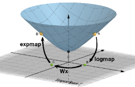
(a) Linear layer formalized in tangent space

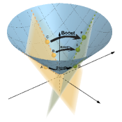
(b) Lorentz boost

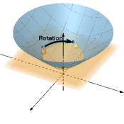
(c) Lorentz rotation

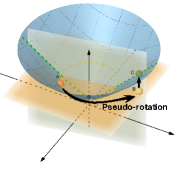
(d) Pseudo-rotation

Figure 1: Illustration of a hyperbolic linear layer based on the logarithmic and exponential maps as well as different transformations in the Lorentz model. In Figure 1a, $A$ is mapped to $B$ in the tangent space at the origin $\mathcal{T}_{\mathbf{0}}\mathbb{L}^{n}_{K}$ through the logarithmic map. A Euclidean linear transformation is performed to obtain $C$. Finally, $C$ is mapped back to the hyperbolic space through the exponential map. Figures 1b and 1c are the visualization of the Lorentz boost and rotation, where points on the intersection of a plane and the hyperboloid are still coplanar after the Lorentz boost. Figure 1d is pseudo-rotation in § 3.1, where a point is first transformed and then projected onto the hyperboloid.

2.2 The Lorentz Transformations

In the special relativity, the Lorentz transformations are a family of linear transformations from a coordinate frame in spacetime to another frame moving at a constant velocity relative to the former. Any Lorentz transformation can be decomposed into a combination of a Lorentz boost and a Lorentz rotation by polar decomposition Moretti (2002).

Definition 1 (Lorentz Boost).

Lorentz boost describes relative motion with constant velocity and without rotation of the spatial coordinate axes. Given a velocity $\mathbf{v}\in\mathbb{R}^{n}$ (ratio to the speed of light), $\lVert\mathbf{v}\rVert<1$ and $\gamma=\frac{1}{\sqrt{1-\lVert\mathbf{v}\rVert^{2}}}$, the Lorentz boost matrices are given by $\mathbf{B}=\left[\begin{array}[]{cccc}\gamma&-\gamma\mathbf{v}^{\intercal}\\ -\gamma\mathbf{v}&\mathbf{I}+\frac{\gamma^{2}}{1+\gamma}\mathbf{v}\mathbf{v}^{\intercal}\\ \end{array}\right]$.

Definition 2 (Lorentz Rotation).

Lorentz rotation is the rotation of the spatial coordinates. The Lorentz rotation matrices are given by $\mathbf{R}=\left[\begin{array}[]{cccc}1&\mathbf{0}^{\intercal}\\ \mathbf{0}&\mathbf{\tilde{R}}\\ \end{array}\right]$, where $\mathbf{\tilde{R}}^{\intercal}\mathbf{\tilde{R}}=\mathbf{I}$ and $\det(\mathbf{\tilde{R}})=1$, i.e., $\mathbf{\tilde{R}}\in\textbf{SO}(n)$ is a special orthogonal matrix.

Both the Lorentz boost and the Lorentz rotation are the linear transformations directly defined in the Lorentz model, i.e., $\forall\mathbf{x}\in\mathbb{L}^{n}_{K},\mathbf{B}\mathbf{x}\in\mathbb{L}^{n}_{K}$ and $\mathbf{R}\mathbf{x}\in\mathbb{L}^{n}_{K}$. Hence, we build fully hyperbolic neural networks on the basis of these two types of transformations in this paper.

3 Fully Hyperbolic Neural Networks

3.1 Fully Hyperbolic Linear Layer

We first introduce our hyperbolic linear layer in the Lorentz model, considering it is the most essential block for neural networks. Although the Lorentz transformations in § 2.2 are linear transformations in the Lorentz model, they cannot be directly used for neural networks. On the one hand, the Lorentz transformations transform coordinate frames without changing the number of dimensions. On the other hand, complicated restrictions of the Lorentz transformations (e.g., special orthogonal matrices for the Lorentz rotation) make computation and optimization problematic. Although the restrictions offer nice properties such as spacetime interval invariant to Lorentz transformation, they are unwanted in neural networks.

A Lorentz linear layer matrix should minimize the loss while subject to $\mathbf{M}\in\mathbb{R}^{(m+1)\times(n+1)}$, $\forall\mathbf{x}\in\mathbb{L}^{n},\mathbf{M}\mathbf{x}\in\mathbb{L}^{m}$. It is a constrained optimization difficult to solve. We instead re-formalize our lorentz linear layer to learn a matrix $\mathbf{M}=\left[\begin{smallmatrix}\mathbf{v}^{\intercal}\\ \mathbf{W}\\ \end{smallmatrix}\right],\mathbf{v}\in\mathbb{R}^{n+1},\mathbf{W}\in\mathbb{R}^{m\times(n+1)}$ satisfying $\forall\mathbf{x}\in\mathbb{L}^{n},f_{\mathbf{x}}(\mathbf{M})\mathbf{x}\in\mathbb{L}^{m}$, where $f_{\mathbf{x}}:\mathbb{R}^{(m+1)\times(n+1)}\rightarrow\mathbb{R}^{(m+1)\times(n+1)}$ should be a function that maps any matrix to a suitable one for the hyperbolic linear layer. Specifically, $\forall\mathbf{x}\in\mathbb{L}^{n}_{K},\mathbf{M}\in\mathbb{R}^{(m+1)\times(n+1)}$, $f_{\mathbf{x}}(\mathbf{M})$ is given as

$$f_{\mathbf{x}}(\mathbf{M})=f_{\mathbf{x}}(\left[\begin{array}[]{c}\mathbf{v}^{\intercal}\\ \mathbf{W}\\ \end{array}\right])=\left[\begin{array}[]{c}\frac{\sqrt{\lVert\mathbf{W}\mathbf{x}\rVert^{2}-1/K}}{\mathbf{v}^{\intercal}\mathbf{x}}\mathbf{v}^{\intercal}\\ \mathbf{W}\\ \end{array}\right],$$ (1)

Theorem 1.

$\forall\mathbf{x}\in\mathbb{L}^{n}_{K},\forall\mathbf{M}\in\mathbb{R}^{(m+1)\times(n+1)}$, we have $f_{\mathbf{x}}(\mathbf{M})\mathbf{x}\in\mathbb{L}^{m}_{K}$.

Proof 1.

One can easily verify that $\forall\mathbf{x}\in\mathbb{L}^{n}_{K}$, we have $\langle f_{\mathbf{x}}(\mathbf{M})\mathbf{x},f_{\mathbf{x}}(\mathbf{M})\mathbf{x}\rangle_{\mathcal{L}}=1/K$, thus $f_{\mathbf{x}}(\mathbf{M})\mathbf{x}\in\mathbb{L}^{m}_{K}$. ∎

Relation to the Lorentz Transformations

In this part, we show that the set of matrices $\{f_{\mathbf{x}}(\mathbf{M})\}$ defined in Eq.(1) contains all Lorentz rotation and boost matrices.

Lemma 1.

In the $n$-dimensional Lorentz model $\mathbb{L}^{n}_{K}$, we denote the set of all Lorentz boost matrices as $\mathcal{B}$ , the set of all Lorentz rotation matrices as $\mathcal{R}$ . Given $\mathbf{x}\in\mathbb{L}^{n}_{K}$, we denote the set of $f_{\mathbf{x}}(\mathbf{M})$ at $\mathbf{x}$ without changing the number of space dimension as $\mathcal{M}_{\mathbf{x}}=\{f_{\mathbf{x}}(\mathbf{M})\mid\mathbf{M}\in\mathbb{R}^{(n+1)\times(n+1)}\}$. $\forall\mathbf{x}\in\mathbb{L}^{n}_{K}$, we have $\mathcal{B}\subseteq\mathcal{M}_{\mathbf{x}}$ and $\mathcal{R}\subseteq\mathcal{M}_{\mathbf{x}}$.

Proof 2.

We first prove $\mathcal{M}_{\mathbf{x}}$ covers all valid transformations.

Considering $\mathcal{A}=\{\mathbf{A}\in\mathbb{R}^{(n+1)\times(n+1)}\mid\forall\mathbf{x}\in\mathbb{L}^{n}_{K}:\langle\mathbf{A}\mathbf{x},\mathbf{A}\mathbf{x}\rangle_{\mathcal{L}}=\frac{1}{K},(\mathbf{Ax})_{0}>0\}$ is the set of all valid transformation matrices in the Lorentz model. Then $\forall\mathbf{A}=\left[\begin{smallmatrix}\mathbf{v}^{\intercal}_{A}\\ \mathbf{W}_{A}\\ \end{smallmatrix}\right]\in\mathcal{A}$, $\mathbf{v}_{A}\in\mathbb{R}^{n+1},\mathbf{W}_{A}\in\mathbb{R}^{n\times(n+1)}$, $\exists\mathbf{x}\in\mathbb{R}^{n+1}\colon\mathbf{v}^{\intercal}\mathbf{x}>0$ and $\lVert\mathbf{W}_{A}\mathbf{x}\rVert^{2}-{(\mathbf{v}^{\intercal}_{A}\mathbf{x})}^{2}=\frac{1}{K}$. Furthermore, $\forall\mathbf{A}\in\mathcal{A}$, we have

$$f_{\mathbf{x}}(\mathbf{A})=f_{\mathbf{x}}(\left[\begin{smallmatrix}\mathbf{v}^{\intercal}_{A}\\ \mathbf{W}_{A}\\ \end{smallmatrix}\right])=\left[\begin{smallmatrix}\frac{\sqrt{\lVert\mathbf{W}_{A}\mathbf{x}\rVert^{2}-1/K}}{\mathbf{v}^{\intercal}_{A}\mathbf{x}}\mathbf{v}_{A}^{\intercal}\\ \mathbf{W}_{A}\\ \end{smallmatrix}\right]=\mathbf{A}.$$

Hence, we can see that $\mathcal{A}\subseteq\mathcal{M}_{\mathbf{x}}$. Since $\mathcal{B}\subseteq\mathcal{A}$ and $\mathcal{R}\subseteq\mathcal{A}$, therefore $\mathcal{B}\subseteq\mathcal{M}_{\mathbf{x}}$ and $\mathcal{R}\subseteq\mathcal{M}_{\mathbf{x}}$. ∎

According to Theorems 1 and 1, both Lorentz boost and rotation can be covered by our linear layer.

Relation to the Linear Layer Formalized in the Tangent Space

In this part, we show that the conventional hyperbolic linear layer formalized in the tangent space at the origin Ganea et al. (2018); Nickel and Kiela (2018) can be considered as a Lorentz transformation with only a special rotation but no boost. Figure 1a visualizes the conventional hyperbolic linear layer.

As shown in Figure 1d, we consider a special setting “pseudo-rotation" of our hyperbolic linear layer. Formally, at the point $\mathbf{x}\in\mathbb{L}^{n}_{K}$, all pseudo-rotation matrices make up the set $\mathcal{P}_{\mathbf{x}}=\big{\{}f_{\mathbf{x}}(\left[\begin{smallmatrix}w&\mathbf{0}^{\intercal}\\ \mathbf{0}&\mathbf{W}\end{smallmatrix}\right])\mathrel{\big{|}}w\in\mathbb{R},\mathbf{W}\in\mathbb{R}^{n\times n}\big{\}}$. As we no longer require the submatrix $\mathbf{W}$ to be a special orthogonal matrix, this setting is a relaxation of the Lorentz rotation.

Formally, given $\mathbf{x}\in\mathbb{L}^{n}_{K}$, the conventional hyperbolic linear layer relies on the logarithmic map to map the point into the tangent space at the origin, a matrix to perform linear transformation in the tangent space, and the exponential map to map the final result back to $\mathbb{L}^{n}_{K}$ . The whole process is

$$\exp_{\mathbf{0}}(\left[\begin{smallmatrix}*&\mathbf{0}^{\intercal}\\ \mathbf{0}&\mathbf{W}\end{smallmatrix}\right]\log_{\mathbf{0}}([\begin{smallmatrix}x_{t}\\ \mathbf{x}_{s}\end{smallmatrix}]))=\left[\begin{smallmatrix}\frac{\cosh(\beta)}{\sqrt{-K}x_{t}}&\mathbf{0}^{\intercal}\\ \mathbf{0}&\frac{\sinh(\beta)\mathbf{W}}{\sqrt{-K}\lVert\mathbf{W}\mathbf{x}_{s}\rVert}\end{smallmatrix}\right][\begin{smallmatrix}x_{t}\\ \mathbf{x}_{s}\end{smallmatrix}],$$ (2)

where $\beta=\frac{\sqrt{-K}\cosh^{-1}(\sqrt{-K}x_{t})}{\sqrt{-Kx_{t}^{2}-1}}\lVert\mathbf{W}\mathbf{x}_{s}\rVert$.

Lemma 2.

$\forall\mathbf{x}\in\mathbb{L}^{n}_{K}$ , we define the set of the outcomes of Eq.(2) as

$$\mathcal{H}_{\mathbf{x}}=\left\{\left[\begin{smallmatrix}\frac{\cosh(\beta)}{\sqrt{-K}x_{t}}&\mathbf{0}^{\intercal}\\ \mathbf{0}&\frac{\sinh(\beta)}{\sqrt{-K}\lVert\mathbf{W}\mathbf{x}_{s}\rVert}\mathbf{W}\end{smallmatrix}\right]\mathrel{\bigg{|}}\mathbf{W}\in\mathbb{R}^{n\times n}\right\},$$

then we have $\mathcal{H}_{\mathbf{x}}\subseteq\mathcal{P}_{\mathbf{x}}$ and $\mathcal{H}_{\mathbf{x}}\cap\mathcal{B}=\{\mathbf{I}\}$.

Proof 3.

$\forall\mathbf{x}\in\mathbb{L}^{n}_{K},\forall\mathbf{H}\in\mathcal{H}_{\mathbf{x}}$, $\mathbf{H}$ has the form $\left[\begin{smallmatrix}w&\mathbf{0}^{\intercal}\\ \mathbf{0}&\mathbf{W}\end{smallmatrix}\right]$, satisfying $\lVert\mathbf{W}\mathbf{x}_{s}\rVert^{2}-{(wx_{t})}^{2}=\frac{1}{K}$ and $wx_{t}>0$. We can verify that

$$f_{\mathbf{x}}(\mathbf{H})=f_{\mathbf{x}}(\left[\begin{smallmatrix}w&\mathbf{0}^{\intercal}\\ \mathbf{0}&\mathbf{W}\end{smallmatrix}\right])=\left[\begin{smallmatrix}\frac{\sqrt{\lVert\mathbf{W}\mathbf{x}_{s}\rVert^{2}-1/K}}{wx_{t}}w&\mathbf{0}^{\intercal}\\ \mathbf{0}&\mathbf{W}\\ \end{smallmatrix}\right]=\mathbf{H}.$$

Hence, $\forall\mathbf{x}\in\mathbb{L}^{n}_{K}$, $\forall\mathbf{H}\in\mathcal{H}_{\mathbf{x}}$, we have $\mathbf{H}=f_{\mathbf{x}}(\mathbf{H})\in\mathcal{P}_{\mathbf{x}}$, and thus $\mathcal{H}_{\mathbf{x}}\subseteq\mathcal{P}_{\mathbf{x}}$. ∎

To prove $\mathcal{H}_{\mathbf{x}}\cap\mathcal{B}={\mathbf{I}}$ is trivial, we do not elaborate here. Therefore, a conventional hyperbolic linear layer can be considered as a special rotation where the time axis is changed according to the space axes to ensure that the output is still in the Lorentz model. Our linear layer is not only fully hyperbolic but also equipped with boost operations to be more expressive. Moreover, without using the complicated logarithmic and exponential maps, our linear layer has better efficiency and stability.

A More General Formula

Here, we give a more general formula of our hyperbolic linear layer based on $f_{\mathbf{x}}(\left[\begin{smallmatrix}\mathbf{v}^{\intercal}\\ \mathbf{W}\\ \end{smallmatrix}\right])\mathbf{x}$, by adding activation, dropout, bias and normalization,

$$\mathbf{y}=\texttt{HL}(\mathbf{x})=\left[\begin{smallmatrix}\sqrt{\lVert\phi(\mathbf{Wx,v})\rVert^{2}-1/K}\\ \phi(\mathbf{W}\mathbf{x},\mathbf{v})\end{smallmatrix}\right],$$ (3)

where $\mathbf{x}\in\mathbb{L}^{n}_{K}$, $\mathbf{v}\in\mathbb{R}^{n+1}$, $\mathbf{W}\in\mathbb{R}^{m\times(n+1)}$, and $\phi$ is an operation function: for the dropout, the function is $\phi(\mathbf{Wx,v})=\mathbf{W}\texttt{dropout}(\mathbf{x})$; for the activation and normalization $\phi(\mathbf{Wx,v})=\frac{\lambda\sigma(\mathbf{v}^{\intercal}\mathbf{x}+b^{\prime})}{\lVert\mathbf{W}h(\mathbf{x})+\mathbf{b}\rVert}(\mathbf{W}h(\mathbf{x)+b})$, where $\sigma$ is the sigmoid function, $\mathbf{b}$ and $b^{\prime}$ are bias terms, $\lambda>0$ controls the scaling range, $h$ is the activation function. We elaborate $\phi(\cdot)$ we use in practice in the appendix.

3.2 Fully Hyperbolic Attention Layer

Attention layers are also important for building networks, especially for the networks of Transformer family Vaswani et al. (2017). We propose an attention module in the Lorentz model. Specifically, we consider the weighted aggregation of a point set $\mathcal{P}=\{\mathbf{x}_{1},\ldots,\mathbf{x}_{|\mathcal{P}|}\}$ as calculating the centroid, whose expected (squared) distance to $\mathcal{P}$ is minimum, i.e. $\operatorname*{arg\,min}_{\bm{\mu}\in\mathbb{L}^{n}_{K}}\sum_{i=1}^{|\mathcal{P}|}\nu_{i}d_{\mathcal{L}}^{2}(\mathbf{x}_{i},\bm{\mu})$, where $\nu_{i}$ is the weight of the $i$-th point. Law et al. (2019) prove that, with squared Lorentzian distance defined as $d^{2}_{\mathcal{L}}(\mathbf{a},\mathbf{b})=2/K-2\langle\mathbf{a},\mathbf{b}\rangle_{\mathcal{L}}$, the centroid w.r.t. the squared Lorentzian distance is given as

$$\bm{\mu} =\texttt{Centroid}\big{(}\{\nu_{1},\ldots,\nu_{|\mathcal{P}|}\},\{\mathbf{x}_{1},\ldots,\mathbf{x}_{|\mathcal{P}|}\}\big{)}$$ (4)

$$=\frac{\sum_{j=1}^{|\mathcal{P}|}\nu_{j}\mathbf{x}_{j}}{\sqrt{-K}\big{|}\lVert\sum_{i=1}^{|\mathcal{P}|}\nu_{i}\mathbf{x}_{i}\rVert_{\mathcal{L}}\big{|}}.$$

Given the query set $\mathcal{Q}=\{\mathbf{q}_{1},\ldots,\mathbf{q}_{|\mathcal{Q}|}\}$, key set $\mathcal{K}=\{\mathbf{k}_{1},\ldots,\mathbf{k}_{|\mathcal{K}|}\}$, and value set $\mathcal{V}=\{\mathbf{v}_{1},\ldots,\mathbf{v}_{|\mathcal{V}|}\}$, where $|\mathcal{K}|=|\mathcal{V}|$, we exploit the squared Lorentzian distance between points to calculate weights. The attention is defined as $\texttt{ATT}(\mathcal{Q},\mathcal{K},\mathcal{V})=\{\bm{\mu}_{1},\ldots,\bm{\mu}_{|\mathcal{Q}|}\}$ and given by:

$$\bm{\mu}_{i} =\frac{\sum_{j=1}^{|\mathcal{K}|}\nu_{ij}\mathbf{v}_{j}}{\sqrt{-K}\big{|}\lVert\sum_{k=1}^{|\mathcal{K}|}\nu_{ik}\mathbf{v}_{k}\rVert_{\mathcal{L}}\big{|}},$$ (5)

$$\nu_{ij} =\frac{\exp(\frac{-d_{\mathcal{L}}^{2}(\mathbf{q}_{i},\mathbf{k}_{j})}{\sqrt{n}})}{\sum_{k=1}^{|\mathcal{K}|}\exp(\frac{-d_{\mathcal{L}}^{2}(\mathbf{q}_{i},\mathbf{k}_{k})}{\sqrt{n}})},$$

where $n$ is the dimension of points. Furthermore, multi-headed attention is defined as $\texttt{MHATT}(\mathcal{Q},\mathcal{K},\mathcal{V})=\{\bm{\mu}_{1},\ldots,\bm{\mu}_{|\mathcal{Q}|}\}$, and $\bm{\mu}_{i}$ is

$$\bm{\mu}_{i} =\texttt{HL}([\bm{\mu}_{i}^{1}|\ldots|\bm{\mu}_{i}^{H}]),$$ (6)

$$\{\bm{\mu}_{1}^{i},\bm{\mu}_{2}^{i},\ldots\} =\texttt{ATT}^{i}(\texttt{HL}_{\mathcal{Q}}^{i}(\mathcal{Q}),\texttt{HL}_{\mathcal{K}}^{i}(\mathcal{K}),\texttt{HL}_{\mathcal{V}}^{i}(\mathcal{V})),$$

where $H$ is the head number, $[\cdot|\ldots|\cdot]$ is the concatenation of multiple vectors, $\texttt{ATT}^{i}(\cdot,\cdot,\cdot)$ is the $i$-th head attention, and $\texttt{HL}_{\mathcal{Q}}^{i}(\cdot)$, $\texttt{HL}_{\mathcal{K}}^{i}(\cdot)$, $\texttt{HL}_{\mathcal{V}}^{i}(\cdot)$ are the hyperbolic linear layers of the $i$-th head attention.

Other intuitive choices for the aggregation in the Lorentz attention module include Fréchet mean Karcher (1977) and Einstein midpoint Ungar (2005). The Fréchet mean is the classical generalization of Euclidean mean. However, it offers no closed-form solution. Solving the Fréchet mean currently requires iterative computation Lou et al. (2020); Gu et al. (2019), which significantly slows down the training and inference, making it impossible to generalize to deep and large model . On the contrary, Lorentz centroid is fast to compute and can be seen as Frechet mean in pseudo-hyperbolic space Law et al. (2019). The computation of the Einstein midpoint requires transformation between Lorentz model and Klein model, bringing in numerical instability. The Lorentz centroid we use minimizes the sum of squared distance in the Lorentz model, while the Einstein midpoint does not possess such property in theory. Also, whether the Einstein midpoint in the Klein model has its geometric interpretation in the Lorentz model remains to be investigated, and it is beyond the scope of our paper. Therefore, we adopt the Lorentz centroid in our Lorentz attention.

3.3 Fully Hyperbolic Residual Layer and Position Encoding Layer

Lorentz Residual

The residual layer is crucial for building deep neural networks. Since there is no well-defined vector addition in the Lorentz model, we assume that each residual layer is preceded by a computational block whose last layer is a Lorentz linear layer, and do the residual-like operation within the preceding Lorentz linear layer of the block as a compromise. Given the input $\mathbf{x}$ of the computational block and the output $\mathbf{o}=f(\mathbf{x})$ before the last Lorentz linear layer of the block, we take $\mathbf{x}$ as the bias of the Lorentz linear layer. Concretely, the final output of the block is

$$\mathbf{y} =\left[\begin{smallmatrix}\sqrt{\lVert\phi(\mathbf{W}\mathbf{o},\mathbf{v},\mathbf{x})\rVert^{2}-1/K}\\ \phi(\mathbf{W}\mathbf{o},\mathbf{v},\mathbf{x})\end{smallmatrix}\right],$$ (7)

$$\phi(\mathbf{W}\mathbf{o},\mathbf{v},\mathbf{x}) =\frac{\lambda\sigma(\mathbf{v}^{\intercal}\mathbf{o})}{\lVert\mathbf{W}h(\mathbf{o})+\mathbf{x}_{s}\rVert}(\mathbf{W}h(\mathbf{o})+\mathbf{x}_{s}),$$

where the symbols have the same meaning as those in Eq.(3).

Lorentz Position Encoding

Some neural networks require positional encoding for their embedding layers, especially those models for NLP tasks. Previous works generally incorporate positional information by adding position embeddings to word embeddings. Given a word embedding $\mathbf{x}$ and its corresponding learnable position embedding $\mathbf{p}$, we add a Lorentz linear layer to transform the word embedding $\mathbf{x}$, by taking the position embedding $\mathbf{p}$ as the bias. The overall process is the same as Eq.(7). Note that the transforming matrix in the Lorentz linear layer is shared across positions. This modification gives us one more $d\times d$ matrix than the Euclidean Transformer. The increase in the number of parameters is negligible compared to the huge parameters of the whole model.

	WN18RR					FB15k-237
Model	#Dims	MRR	H@10	H@3	H@1	#Dims	MRR	H@10	H@3	H@1
TransE Bordes et al. (2013)	180	22.7	50.6	38.6	3.5	200	28.0	48.0	32.1	17.7
DistMult Yang et al. (2015)	270	41.5	48.5	43.0	38.1	200	19.3	35.3	20.8	11.5
ComplEx Trouillon et al. (2017)	230	43.2	50.0	45.2	39.6	200	25.7	44.3	29.3	16.5
ConvE Dettmers et al. (2018)	120	43.5	50.0	44.6	40.1	200	30.4	49.0	33.5	21.3
RotatE Sun et al. (2019)	1,000	47.3	55.3	48.8	43.2	1,024	30.1	48.5	33.1	21.0
TuckER Balazevic et al. (2019b)	200	46.1	53.5	47.8	42.3	200	34.7	53.3	38.4	25.4
MuRP Balazevic et al. (2019a)	32	46.5	54.4	48.4	42.0	32	32.3	50.1	35.3	23.5
RotH Chami et al. (2020a)	32	47.2	55.3	49.0	42.8	32	31.4	49.7	34.6	22.3
AttH Chami et al. (2020a)	32	46.6	55.1	48.4	41.9	32	32.4	50.1	35.4	23.6
HyboNet	32	48.9	55.3	50.3	45.5	32	33.4	51.6	36.5	24.4
MuRP Balazevic et al. (2019a)	$\beta$	48.1	56.6	49.5	44.0	$\beta$	33.5	51.8	36.7	24.3
RotH Chami et al. (2020a)	$\beta$	49.6	58.6	51.4	44.9	$\beta$	34.4	53.5	38.0	24.6
AttH Chami et al. (2020a)	$\beta$	48.6	57.3	49.9	44.3	$\beta$	34.8	54.0	38.4	25.2
HyboNet	$\beta$	51.3	56.9	52.7	48.2	$\beta$	35.2	52.9	38.7	26.3

Table 1: Link prediction results (%) on WN18RR and FB15k-237 in the filtered setting. $\beta\in\{200,400,500\}$ and we report the best result. The first group of models are Euclidean models, the second and third groups are hyperbolic models with different dimensions. Following Balazevic et al. (2019a), RotatE results are reported without their self-adversarial negative sampling for fair comparison. Best results are in bold. Best results among hyperbolic networks with same dimensions are underlined.

4 Experiments

To verify our proposed framework, we conduct experiments on both shallow and deep neural networks. For shallow neural networks, we present results on knowledge graph completion. For deep neural networks, we propose a Lorentz Transformer and present results on machine translation. Dependency tree probing is also done on both Lorentz and Euclidean Transformers to compare their capabilities of representing structured information. Due to space limitations, we report the results of network embedding and fine-grained entity typing experiments in the appendix A. For knowledge graph completion and network embedding, we use our fully hyperbolic linear layer, and for other tasks, we use the general formula given in § 3.1, which is a relaxation of our fully hyperbolic linear layer.

In the following sections, we denote the models built with our proposed framework as HyboNet. We demonstrate that HyboNet not only outperforms Euclidean and Poincaré models on the majority of tasks, but also converges better than its Poincaré counterpart. All models in § 4.1 are trained with $1$ NVIDIA 2080Ti, models in § 4.2 are trained with $1$ NVIDIA 40GB A100 GPU. We optimize our model with Riemannian Adam Kochurov et al. (2020). For pre-processing and hyper-parameters of each experiment, please refer to Appendix B.

4.1 Experiments on Shallow Networks

In this part, we leverage our Lorentz embedding and linear layers to build shallow neural networks. We show that HyboNet outperforms previous knowledge graph completion models on several popular benchmarks.

4.1.1 Knowledge Graph Completion Models

A knowledge graph contains a collection of factual triplets, each triplet ($h,r,t$) illustrates the existence of a relation $r$ between the head entity $h$ and the tail entity $t$. Since knowledge graphs are generally incomplete, predicting missing triplets becomes a fundamental research problem. Concretely, the task aims to solve the problem ($h,r,?$) and ($?,r,t$).

We use two popular knowledge graph completion benchmarks, FB15k-237Toutanova and Chen (2015) and WN18RRDettmers et al. (2018) in our experiments. We report two evaluation metrics: MRR (Mean reciprocal rank), the average of the inverse of the true entity ranking in the prediction; H@$\mathbf{K}$, the percentage of the correct entities appearing within the top $K$ positions of the predicted ranking.

(a) WN18RR

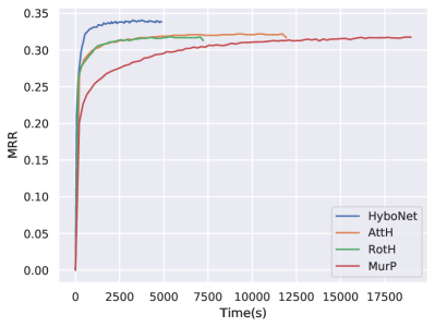
(b) FB15k-237

Figure 2: Validation curves of knowledge graph models.

Setup Similar to Balazevic et al. (2019a), we design a score function for each triplet as

$$s(h,r,t) =-d_{\mathcal{L}}^{2}(f_{r}(\mathbf{e}_{h}),\mathbf{e}_{t})+b_{h}+b_{t}+\delta,$$

where $\mathbf{e}_{h},\mathbf{e}_{t}\in\mathbb{L}^{n}_{K}$ are the Lorentz embeddings of the head entity $h$ and the tail entity $t$, $f_{r}(\cdot)$ is a Lorentz linear transformation of the relation $r$ and $\delta$ is a margin hyper-parameter. For each triplet, we randomly corrupt its head or tail entity with $k$ entities and calculate the probabilities for triplets as $p=\sigma(s(h,r,t))$, where $\sigma$ is the sigmoid function. Finally, we minimize the binary cross entropy loss

$$\mathcal{L}=-\frac{1}{N}\sum_{i=1}^{N}\left(\log p^{(i)}+\sum_{j=1}^{k}\log(1-\tilde{p}^{(i,j)})\right),$$

where $p^{(i)}$ and $\tilde{p}^{(i,j)}$ are the probabilities for correct and corrupted triplets respectively, $N$ is the triplet number. We select the model with the best MRR on validation set and report its performance on test set.

Results Table 1 shows the results on both datasets. As expected, low-dimensional hyperbolic networks have already achieved comparable or even better results when compared to high-dimensional Euclidean baselines. When the dimensionality is raised to a maximum of 500, HyboNet outperforms all other baselines on MRR, H@3, and H@1 by a significant margin. And as shown in Figures 2a and 2b, HyboNet converges better than other hyperbolic networks on both datasets and has a higher ceiling, demonstrating the superiority of our Lorentz linear layer over conventional linear layer formalized in tangent space.

4.2 Experiments on Deep Networks

In this part, we build a Transformer Vaswani et al. (2017) with our Lorentz components introduced in § 3. We omit layer normalization for the difficulty of defining hyperbolic mean and variance, but it is still kept in our Euclidean Transformer baseline. In fact, $\lambda$ in Eq.(3) controls the scaling range, which normalize the representations to some extent.

4.2.1 Machine Translation

We conduct the experiment on two widely-used machine translation benchmarks: IWSLT’14 English-German and WMT’14 English-German.

Setup

We use OpenNMT Klein et al. (2017) to build Euclidean Transformer and our Lorentz one. Following previous hyperbolic work Shimizu et al. (2021), we conduct experiments in low-dimensional settings. To show that our framework can be applied to high-dimensional settings, we additionally train a Lorentz Transformer of the same size as Transformer base, and compare their performance on WMT’14. We select the model with the lowest perplexity on the validation set, and report its BLEU scores on the test set.

Results

The BLEU scores on the test set of IWSLT’14 and newstest2013 test set of WMT’14 are shown in Table 2. Both Transformer-based hyperbolic models, HyboNet and HAtt Gulcehre et al. (2018), outperform the Euclidean Transformer. However, in HAtt, only the calculation of attention weights and the aggregation are performed in hyperbolic space, leaving the remaining computational blocks in the Euclidean space. That is, HAtt is a partially hyperbolic Transformer. As a result, the merits of hyperbolic space are not fully exploited. On the contrary, HyboNet performs all its operations in the hyperbolic space, thus better utilizes the hyperbolic space, and achieve significant improvement over both Euclidean and partially hyperbolic Transformer. Apart from the low-dimensional setting that is common in hyperbolic literature, we scale up the model to be the same size as Transformer base (512-dimensional input) Vaswani et al. (2017). We report the results in Table 3. HyboNet outperforms Transformer and HAtt with the same model size, and is very close to the much bigger Transformer${}_{\text{big}}$.

4.2.2 Dependency Tree Probing

	IWSLT’14	WMT’14
Model	d=64	d=64	d=128	d=256
ConvSeq2Seq	23.6	14.9	20.0	21.8
Transformer	23.0	17.0	21.7	25.1
HyperNN++	22.0	17.0	19.4	21.8
HAtt	23.7	18.8	22.5	25.5
HyboNet	25.9	19.7	23.3	26.2

Table 2: The BLEU scores on the test set of IWSLT’14 and WMT’14 under the low-dimensional setting.

Model	WMT’14
Transformer${}_{\text{base}}$ Vaswani et al. (2017)	27.3
Transformer${}_{\text{big}}$ Vaswani et al. (2017)	28.4
HAtt${}_{\text{base}}$ Gulcehre et al. (2018)	27.5
HyboNet${}_{\text{base}}$	28.2

Table 3: The BLEU scores on the test set of WMT’14 under the high-dimensional setting. The results of Transformer and HAtt are taken from their original paper respectively.

In this part, we verify the superiority of HyboNet in capturing latent structured information in unstructured sentences through dependency tree probing. It has been shown that neural networks implicitly embed syntax trees in their intermediate context representations Hewitt and Manning (2019); Raganato et al. (2018). One reason we think HyboNet performs better in machine translation is that it better captures structured information in the sentences. To validate this, we perform a probing on Transformer, HAtt and HyboNet obtained in § 4.2.1. We use dependency parsing result of stanza Qi et al. (2020) on IWSLT’14 English corpus as our dataset. The data partition is kept.

Setup

For a fair comparison, we probe all the models in hyperbolic space following Chen et al. (2021). Four metrics are reported: UUAS (undirected attachment score), the percentage of undirected edges placed correctly against the gold tree; Root%, the precision of the model predicting the root of the syntactic tree; Dspr. and Nspr., the Spearman correlations between true and predicted distances for each word in each sentence, true depth ordering and the predicted ordering, respectively. Please refer to the appendix for details.

	Distance		Depth
Model	UUAS	Dspr.	Root%	Nspr.
Transformer	0.36	0.30	12	0.88
HAtt	0.50	0.64	49	0.88
HyboNet	0.59	0.70	64	0.92

Table 4: The probing results on dependency tree constructed from the Iwslt’14 English corpus.

Results

The probing results are shown in Table 2. HyboNet outperforms other baselines by a large margin. Obviously, syntax trees can be better reconstructed from the intermediate representation of HyboNet’s encoder, which shows that HyboNet better captures syntax structure. The result of HAtt is also worth noting. Because HAtt is a partially hyperbolic Transformer, intuitively, its ability to capture the structured information should be better than Euclidean Transformer, but worse than HyboNet. Our result confirms this suspicion indeed. The probing on HAtt indicates that as the model becomes more hyperbolic, the ability to learn structured information becomes stronger.

5 Related Work

Hyperbolic geometry has been widely investigated in representation learning in recent years, due to its great expression capacity in modeling complex data with non-Euclidean properties. Previous works have shown that when handling data with hierarchy, hyperbolic embedding has better representation capacity and generalization ability Cvetkovski and Crovella (2016); Verbeek and Suri (2014); Walter (2004); Kleinberg (2007); Krioukov et al. (2009); Cvetkovski and Crovella (2009); Shavitt and Tankel (2008); Sarkar (2011). Moreover, Ganea et al. (2018) and Nickel and Kiela (2018) introduce the basic operations of neural networks in the Poincaré ball and the Lorentz model respectively. After that, researchers further introduce various types of neural models in hyperbolic space including hyperbolic attention networks (Gulcehre et al., 2018), hyperbolic graph neural networks (Liu et al., 2019; Chami et al., 2019), hyperbolic prototypical networks (Mettes et al., 2019) and hyperbolic capsule networks (Chen et al., 2020). Recently, with the rapid development of hyperbolic neural networks, people attempt to utilize them in various downstream tasks such as word embeddings (Tifrea et al., 2018), knowledge graph embeddings (Chami et al., 2020b), entity typing López et al. (2019), text classification (Zhu et al., 2020), question answering (Tay et al., 2018) and machine translation (Gulcehre et al., 2018; Shimizu et al., 2021), to handle their non-Euclidean properties, and have achieved significant and consistent improvement.

Our work not only focus on the improvement in the downstream tasks that hyperbolic space offers, but also show that hyperbolic linear transformation used in previous work is just a relaxation of Lorentz rotation, giving a different theoretical interpretation for the hyperbolic linear transformation.

6 Conclusion and Future Work

In this work, we propose a novel fully hyperbolic framework based on the Lorentz transformations to overcome the problem that hybrid architectures of existing hyperbolic neural networks relied on the tangent space limit network capabilities. The experimental results on several representative NLP tasks show that compared with other hyperbolic networks, HyboNet has faster speed, better convergence, and higher performance. In addition, we also observe that some challenging problems require further efforts: (1) Though we have verified the effectiveness of fully hyperbolic models in NLP, exploring its applications in computer vision is still a valuable direction. (2) Though HyboNet has better performance on many tasks, it is slower than Euclidean networks. Also, because of the floating-point error, HyboNet cannot be sped up with half precision training. We hope more efforts can be devoted into this promising field.

Appendix A Other Experiments

A.1 Graph Neural Networks

Previous works have shown that when equipped with hyperbolic geometry, GNNs demonstrate impressive improvements compared with its Euclidean counterparts Chami et al. (2019); Liu et al. (2019). In this part, we extend GCNs with our proposed hyperbolic framework. Following Chami et al. (2019), we evaluate our HyboNet for link prediction and node classification on four network embedding datasets, and observe better or comparable results as compared to previous methods.

Setup

The architecture of GCNs can be summarized into three parts: feature transformation, neighborhood aggregation and non-linear activation. We use a Lorentz linear layer for the feature transformation, and use the centroid of neighboring node features as the aggregation result. The non-linear activation is integrated into Lorentz linear layer as elaborated in § 3.1. The overall operations of the $l$-th network layer can be formulated into the following manner:

$$\mathbf{x}_{i}^{l}=\texttt{Att}(\texttt{HL}(\mathbf{x}_{i}^{l-1}),\{\texttt{HL}(\mathbf{x}_{j\in\mathcal{N}(i)}^{l-1})\},\{\texttt{HL}(\mathbf{x}_{j\in\mathcal{N}(i)}^{l-1})\}),$$

where $\mathbf{x}_{i}^{l}$ refers to the representation of the $i$-th node at the layer $l$, $\mathcal{N}(i)$ denotes the neighboring nodes of the $i$-th node. With the node representation, we can easily conduct link prediction and node classification. For link prediction, we calculate the probability of edges using Fermi-Dirac decoder Krioukov et al. (2010); Nickel and Kiela (2017):

$$p((i,j)\in\mathcal{E}\mid\mathbf{x}_{i},\mathbf{x}_{j})=\left(\exp((d^{2}_{\mathcal{L}}(\mathbf{x}_{i},\mathbf{x}_{j})-r)/t)+1\right)^{-1},$$ (8)

where $r$ and $t$ are hyper-parameters. We minimize the binary cross entropy loss. For node classification, we calculate the squared Lorentzian distance between node representation and class representations, and minimize the cross entropy loss.

	Disease($\delta=0$)		Airport($\delta=1$)		PubMed($\delta=3.5$)		Cora($\delta=11$)
Task	LP	NC	LP	NC	LP	NC	LP	NC
GCN Kipf and Welling (2017)	64.7±0.5	69.7±0.4	89.3±0.4	81.4±0.6	91.1±0.5	78.1±0.2	90.4±0.2	81.3±0.3
GAT Veličković et al. (2018)	69.8±0.3	70.4±0.4	90.5±0.3	81.5±0.3	91.2±0.1	79.0±0.3	93.7±0.1	83.0±0.7
SAGE Hamilton et al. (2017)	65.9±0.3	69.1±0.6	90.4±0.5	82.1±0.5	86.2±1.0	77.4±2.2	85.5±0.6	77.9±2.4
SGC Wilson et al. (2014)	65.1±0.2	69.5±0.2	89.8±0.3	80.6±0.1	94.1±0.0	78.9±0.0	91.5±0.1	81.0±0.1
HGCN Chami et al. (2019)	91.2±0.6	82.8±0.8	96.4±0.1	90.6±0.2	96.1±0.2	78.4±0.4	93.1±0.4	81.3±0.6
HAT Zhang et al. (2021a)	91.8±0.5	83.6±0.9	/	/	96.0±0.3	78.6±0.5	93.0±0.3	83.1±0.6
LGCN Zhang et al. (2021b)	96.6±0.6	84.4±0.8	96.0±0.6	90.9±1.7	96.8±0.1	78.6±0.7	93.6±0.4	83.3±0.7
HyboNet	96.8±0.4	96.0±1.0	97.3±0.3	90.9±1.4	95.8±0.2	78.0±1.0	93.6±0.3	80.2±1.3

Table 5: Test ROC AUC results (%) for Link Prediction (LP) and F1 scores (%) for Node Classification (NC). HGCN and HyboNet are hyperbolic models. $\delta$ refers to Gromovs $\delta$-hyperbolicity, and is given by Chami et al. (2019). The lower the $\delta$, the more hyperbolic the graph.

Results

Following Chami et al. (2019), we report ROC AUC results for link prediction and F1 scores for node classification on four different network embedding datasets. The description of the datasets can be found in our appendix. Chami et al. (2019) compute Gromovs $\delta$-hyperbolicityJonckheere et al. (2008); Adcock et al. (2013); Narayan and Saniee (2011) for these four datasets. The lower the $\delta$ is, the more hyperbolic the graph is.

The results are reported in Table 5. HyboNet outperforms other baselines in those highly hyperbolic datasets. For Disease dataset, HyboNet even achieves a 12% (absolute) improvement on node classification over previous hyperbolic GCNs. On the less hyperbolic datasets such as PubMed and Cora, HyboNet still performs well on link prediction, and remains competitive for node classification. Although HyboNet does not significantly better than LGCN on all datasets, we observe that HyboNet is far more stable than LGCN. Out of 128 link prediction experiments in grid search, there are 89 times that LGCN generates NaN and fails to finish training, while HyboNet remains stable and is faster than LGCN.

A.2 Fine-grained Entity Typing

Given a sentence containing a mention of entity $e$, the purpose of entity typing is to predict the type of $e$ from a type inventory. It is a multi-label classification problem since multiple types can be assigned to $e$. For fine-grained entity typing, type labels are divided into finer granularity, making the type inventory contains thousands of types. We conduct the experiment on Open Entity dataset Choi et al. (2018), which divides types into three levels: coarse, fine, and ultra-fine.

Model	Total	C	F	UF	#Para
LabelGCN	35.8	67.5	42.2	21.3	5.1M
MultiTask	31.0	61.0	39.0	14.0	6.1M
HY Base	36.3	68.1	38.9	21.2	1.8M
HY Large	37.4	67.6	41.4	24.7	4.6M
HY xLarge	38.2	67.1	40.4	25.7	9.5M
Lorentz (Tangent)	37.2	68.0	40.3	22.4	2.9M
HyboNet	38.2	68.1	43.2	23.5	2.9M

Table 6: Macro $F_{1}$ scores (%) on the development set of Open Entity dataset for different baselines and models. Best results are underlined, and best results among hyperbolic models are in bold.

Setup

Our entity typing model consists of a mention encoder and a context encoder. To get mention representation, the mention encoder first obtain word representation $\mathbf{s}_{i}$, then calculate the centroid of $\mathbf{s}_{i}$ as mention representation $\mathbf{m}$ according to Eq. (4) with uniform weight. The context encoder is a Lorentz Transformer encoder that shares the same embedding module with mention encoder. The context representation $\mathbf{c}$ is the distance-based attention López and Strube (2020) result over the Transformer encoder’s output. We combine $\mathbf{m}$ and $\mathbf{c}$ in the way of combining multi-headed outputs described in § 3.2 by regarding $\mathbf{m}$ and $\mathbf{c}$ as a two-headed output. We then calculate a probability $p_{i}=\sigma(-d_{\mathcal{L}}^{2}(\mathbf{r},\mathbf{t}_{i})/\alpha_{i}+\beta_{i})$ for every type label, where $\sigma$ is sigmoid function, $\mathbf{t}_{i}$ is the Lorentz embedding of the $i$-th type label, and $\alpha_{i},\beta_{i}$ are learnable scale and bias factor respectively. During training, we optimize the multi-task objective Vaswani et al. (2017). For evaluation, a type is predicted if its probability is larger than $0.5$.

Results

Following previous works Choi et al. (2018); López and Strube (2020), we report the macro-averaged F1 scores on the development set of Open Entity dataset in Table 6. HyboNet outperforms LabelGCN Xiong et al. (2019) and MultiTask Vaswani et al. (2017) on Total with fewer parameters. Compared with large Euclidean models Denoised and BERT, HyboNet achieves comparable fine and ultra-fine results with significantly fewer parameters. Compared with another hyperbolic model HY López and Strube (2020), which is based on the Poincaré ball model, HyboNet outperforms HY xLarge model on coarse and fine results. Note that HyboNet has only slightly more parameters than HY base, and fewer than HY Large.

Appendix B Data Preprocessing Methods

We describe data preprocessing methods for each experiment in this section.

B.1 Knowledge Graph Completion

The statistics of WN18RR and FB15k-237 are listed in Table 7. We keep our data preprocessing method for knowledge graph completion the same as Balazevic et al. (2019a). Concretely, we augment both WN18RR and FB15k-237 by adding reciprocal relations for every triplet, i.e. for every ($h,r,t$) in the dataset, we add an additional triplet ($t,r^{-1},h$).

B.2 Machine Translation

For WMT’14, we use the preprocessing script provided by OpenNMT. For IWSLT’14, we clean and partition the dataset with script provided by FairSeq. We limit the lengths of both source and target sentences to be 100 and do not share the vocabulary between source and target language.

B.3 Network Embedding

We use four datasets, referred to as Disease, Airport, Pubmed and Cora. The four datasets are preprocessed by Chami et al. (2019) and published in their code repository. We refer the readers to Chami et al. (2019) for further information about the datasets.

B.4 Entity Typing

The dataset consist of $6,000$ crowd sourced samples and $6$M distantly supervised training samples. We keep our data preprocessing method for knowledge graph completion the same as López and Strube (2020). For the input context, We trimmed the sentence to a maximum of 25 words. During the trimming, one word at a time is removed from one side of the mention, trying to keep the mention in the center of the sentence, and preserve the context information of the mention. For the input mention, we trimmed the mention to a maximum of 5 words.

Appendix C Experiment Details

All of our experiments use 32-bit floating point numbers, not 64-bit floating point numbers as in most previous work. We use PyTorch as the neural networks’ framework. The negative curvature $K$ of the Lorentz model in our experiments is $-1$.

We take the function $\phi$ in Lorentz linear layer to have the form

$$\phi(\mathbf{Wx})=\frac{\sqrt{(\lambda\sigma(\mathbf{v}^{T}\mathbf{x}+b)+\epsilon)^{2}+1/K}}{\lVert\mathbf{W}h\big{(}\texttt{dropout}(\mathbf{x})\big{)}\rVert}\mathbf{W}h\big{(}\texttt{dropout}(\mathbf{x})\big{)}.$$ (9)

To see what it means, we first compute $\mathbf{y}_{0}=\lambda\sigma(\mathbf{v}^{T}\mathbf{x}+b)+\epsilon$ as the $0$-th dimension of the output $\mathbf{y}$, where $\sigma$ is the sigmoid function, $\lambda$ controls the $0$-th dimension’s range, it can be either learnable or fixed, $b$ is a learnable bias term, and $\epsilon>\sqrt{1/K}$ is a constant preventing the $0$-th dimension be smaller than $\sqrt{1/K}$. According to the definition of Lorentz model, $\mathbf{y}$ should satisfies $\lVert\mathbf{y}_{1:n}\rVert^{2}-\mathbf{y_{0}}^{2}=1/K$, that is, $\lVert\mathbf{y}_{1:n}\rVert=\sqrt{\mathbf{y_{0}}^{2}+1/K}=\sqrt{(\lambda\sigma(\mathbf{v}^{T}\mathbf{x}+b)+\epsilon)^{2}+1/K}$. Then equation 9 can be seen as first calculate $\tilde{\mathbf{y}}_{1:n}=\mathbf{W}h\big{(}\texttt{dropout}(\mathbf{x})\big{)}$, then scale $\tilde{\mathbf{y}}_{1:n}$ to have vector norm $\lVert\mathbf{y}_{1:n}\rVert$ to obtain $\mathbf{y}_{1:n}$. Finally, we concatenate $\mathbf{y_{0}}$ with $\mathbf{y}_{1:n}$ as output.

For residual and position embedding addition, we also use Eq.(9).

C.1 Initialization

Dataset	#Ent	#Rel	#Train	#Valid	#Test
FB15k-237	14,541	237	272,115	17,535	20,466
WN18RR	40,943	11	86,835	3,034	3,134

Table 7: Statistics of FB15k-237 and WN18RR.

Embedding
$\mathbf{x}_{i}$	Geoopt default
Parameters in $f$	Uniform(-0.02, 0.02)
Lorentz Linear Layer
$\mathbf{W}$	Uniform(-0.02, 0.02)
$\mathbf{v}$	Uniform(-0.02, 0.02)

Table 8: Initialization methods of different parameters.

We use different initialization method for different parameters, see Table 8. GeooptKochurov et al. (2020) initialize the parameter with Gaussian distribution in the tangent space, and map the embedding to hyperbolic space with exponential map.

C.2 Knowledge Graph Completion

	WN18RR		FB15k-237
Dimension	32	500	32	500
Batch Size	1000	1000	500	500
Neg Samples	50	50	50	50
Margin	8.0	8.0	8.0	8.0
Epochs	1000	1000	500	500
Max Norm	1.5	2.5	1.5	1.5
$\lambda$	3.5	2.5	2.5	2.5
Learning Rate	0.005	0.003	0.003	0.003
Grad Norm	0.5	0.5	0.5	0.5
Optimizer	rAdam	rAdam	rAdam	rAdam

Table 9: Hyper-parameters for knowldge graph completion.

	Disease($\delta=0$)		Airport($\delta=1$)		PubMed($\delta=3.5$)		Cora($\delta=11$)
Task	LP	NC	LP	NC	LP	NC	LP	NC
Learning Rate	0.005	0.005	0.01	0.02	0.008	0.02	0.02	0.02
Weight Decay	0	0	0.002	0.0001	0	0.001	0.001	0.01
Dropout	0.0	0.1	0.0	0.0	0.5	0.8	0.7	0.9
Layers	2	4	2	6	2	3	2	3
Max Grad Norm	None	0.5	0.5	1	0.5	0.5	0.5	1

Table 10: Hyper-parameters for network embeddings.

We list the hyper-parameters used in the experiment in Table 9. Note that in this experiment, we restrict the norm of the last $n$ dimension of the embeddings to be no bigger than a certain value, referred to as Max Norm in Table 9. For each dataset, we explore $\text{BatchSize}\in\{500,1000\}$, $\text{Margin}\in\{4,6,8\}$, $\text{MaxNorm}\in\{1.5,2.5,3.5\}$, $\lambda\in\{2.5,3.5,5.5\}$, $\text{LearningRate}\in\{3e-3,5e-3,7e-3\}$.

Hyper-parameter	IWSLT’14	WMT’16
GPU Numbers	1	4	4	4
Embedding Dimension	64	64	128	256
Feed-forward Dimension	256	256	512	1024
Batch Type	Token	Token	Token	Token
Batch Size Per GPU	10240	10240	10240	10240
Gradient Accumulation Steps	1	1	1	1
Training Steps	40000	200000	200000	200000
Dropout	0.0	0.1	0.1	0.1
Attention Dropout	0.1	0.0	0.0	0.0
Max Gradient Norm	0.5	0.5	0.5	0.5
Warmup Steps	8000	6000	6000	6000
Decay Method	noam	noam	noam	noam
Label Smoothing	0.1	0.1	0.1	0.1
Layer Number	6	6	6	6
Head Number	4	4	8	8
Learning Rate	5	5	5	5
Optimizer	rAdam	rAdam	rAdam	rAdam

Table 11: Hyper-parameters for machine translation.

C.3 Machine Translation

Our code is based on OpenNMT’s TransformerKlein et al. (2017). The hyper-parameters are listed in Table 11

C.4 Dependency Tree Probing

The probing for the Euclidean Transformer is done by first applying an Euclidean linear mapping $f_{P}:\mathbb{R}^{n}\rightarrow\mathbb{R}^{m+1}$ followed by a projection to map Transformer’s intermediate context-aware representation $\mathbf{c}_{i}$ into points $\mathbf{\tilde{h}}_{i}$ in tangent space of Lorentz model’s origin, then using exponential map to map $\mathbf{\tilde{h}}_{i}$ to hyperbolic space $\mathbf{p}_{i}$. In the hyperbolic space, we construct the Lorentz syntactic subspace via a Lorentz linear layer $f_{Q}:\mathbb{L}_{K}^{m}\rightarrow\mathbb{L}_{K}^{m}$:

$$\mathbf{p}_{i} =\exp_{\mathbf{0}}^{K}(f_{P}(\mathbf{c}_{i})),$$

$$\mathbf{q}_{i} =f_{Q}(\mathbf{p}_{i}).$$

We use the squared Lorentzian distance between $\mathbf{q}_{i}$ and $\mathbf{q}_{j}$ to recreate tree distances between word pairs $w_{i}$ and $w_{j}$, the squared Lorentzian distance between $\mathbf{q}_{i}$ and the origin $\mathbf{o}$ to recreate the depth of word $w_{i}$. We minimize the following loss:

$$\mathcal{L}_{\text{distance}} =\frac{1}{l^{2}}\sum_{i,j\in\{1,\cdots,t\}}|d_{T}(w_{i},w_{j})-d_{\mathcal{L}}^{2}(\mathbf{q}_{i},\mathbf{q}_{j})|$$

$$\mathcal{L}_{\text{depth}} =\frac{1}{l}\sum_{i\in\{1,\cdots,t\}}|d_{D}(w_{i})-d_{\mathcal{L}}^{2}(\mathbf{q}_{i},\mathbf{o})|,$$

where $d_{T}(w_{i},w_{j})$ is the edge number of the shortest path from $w_{i}$ to $w_{j}$ in the dependency tree, and $l$ is the sentence length. For the probing of Lorentz Transformer, we only substitute $f_{P}$ with a Lorentz one, and discard the exponential map. We probe every layer for both models, and report the results of the best layer.

We do the probing in the 64 dimensional hyperbolic space. The hyper-parameters and the best layer we choose according to development set are listed in Table 12. Because no Lorentz embedding is involved, we simply use Adam as the optimizer. For parameter selection, we explore $\text{Learning Rate}\in\{5e-4,3e-4,1e-4,5e-5,3e-5,1e-5\}$, $\text{Weight Decay}\in\{0,1e-6,1e-5,1e-4\}$, Batch Size$\in\{16,32,64\}$.

C.5 Network Embedding

The experiment setting is the same as Chami et al. (2019). We list the hyper-parameters for the four datasets in Table.10

C.6 Entity Typing

We initialize the word embeddings by isometrically projecting the pretrained Poincaré Glove word embeddings Tifrea et al. (2018) to Lorentz model, and fix them during training. A Lorentz linear layer is applied to transform the word embeddings to a higher dimension. To get mention representation, the mention encoder first obtain word representation $\mathbf{s}_{i}$ through position encoding module described in section 3.4, then calculate the centroid of $\mathbf{s}_{i}$ as mention representation $\mathbf{m}_{i}$ according to Eq. 14 with uniform weight

$$\mathbf{s}_{i} =\texttt{PE}(\texttt{HL}(\mathbf{w}_{i})),$$

$$\mathbf{m}_{i} =\texttt{Centroid}(1/l,\mathbf{s}_{i}),$$

where $l$ is the length of sentence, $\mathbf{w}_{i}$ is the pretrained embedding of $i$-th word. The context encoder is a Lorentz Transformer encoder that shares the same embedding module with mention encoder. The context representation $\mathbf{c}$ is the distance-based attention López and Strube (2020) result over the Transformer encoder’s output $\mathbf{h}_{i}$:

$$\mathbf{x}_{i}=\texttt{PE}(\mathbf{h}_{i}) ,\quad\mathbf{q}_{i}=\texttt{HL}(\mathbf{x}_{i}),\quad\mathbf{k}_{i}=\texttt{HL}(\mathbf{x}_{i}),$$

$$\nu_{ij} =\texttt{Softmax}(-d_{\mathcal{L}}^{2}(\mathbf{q}_{i},\mathbf{k}_{j})/\sqrt{n}),$$

$$\mathbf{c} =\texttt{Centroid}(\nu_{ij},\mathbf{h}_{i}).$$

Table 12: Hyper-parameters for dependency tree probing.

Hyper-parameter	Euclidean	HAtt	HyboNet
Learning Rate	5e-5	5e-5	5e-5
Weight Decay	0	1e-6	0
Best Layer	0	3	4
Batch Size	64	32	32
Steps	20000	20000	20000
Optimizer	Adam	Adam	Adam

References

- Adcock et al. (2013) Aaron B Adcock, Blair D Sullivan, and Michael W Mahoney. 2013. Tree-like structure in large social and information networks. In Proceedings of ICDM, pages 1–10. IEEE Computer Society.
- Balazevic et al. (2019a) Ivana Balazevic, Carl Allen, and Timothy Hospedales. 2019a. Multi-relational poincaré graph embeddings. In Proceedings of NeurIPS, pages 4463–4473.
- Balazevic et al. (2019b) Ivana Balazevic, Carl Allen, and Timothy Hospedales. 2019b. Tucker: Tensor factorization for knowledge graph completion. In Proceedings of EMNLP-IJCNLP, pages 5188–5197.
- Bordes et al. (2013) Antoine Bordes, Nicolas Usunier, Alberto Garcia-Durán, Jason Weston, and Oksana Yakhnenko. 2013. Translating embeddings for modeling multi-relational data. In Proceedings of ICONIP, pages 2787–2795.
- Bose et al. (2020) Joey Bose, Ariella Smofsky, Renjie Liao, Prakash Panangaden, and Will Hamilton. 2020. Latent variable modelling with hyperbolic normalizing flows. In Proceedings of ICML, pages 1045–1055. PMLR.
- Chami et al. (2020a) Ines Chami, Adva Wolf, Da-Cheng Juan, Frederic Sala, Sujith Ravi, and Christopher Ré. 2020a. Low-dimensional hyperbolic knowledge graph embeddings. In Proceedings of ACL, pages 6901–6914.
- Chami et al. (2020b) Ines Chami, Adva Wolf, Da-Cheng Juan, Frederic Sala, Sujith Ravi, and Christopher Ré. 2020b. Low-dimensional hyperbolic knowledge graph embeddings. In Proceedings of ACL, pages 6901–6914.
- Chami et al. (2019) Ines Chami, Zhitao Ying, Christopher Ré, and Jure Leskovec. 2019. Hyperbolic graph convolutional neural networks. In Proceedings of NeurIps, pages 4869–4880.
- Chen et al. (2021) Boli Chen, Yao Fu, Guangwei Xu, Pengjun Xie, Chuanqi Tan, Mosha Chen, and Liping Jing. 2021. Probing {bert} in hyperbolic spaces. In Proceedings of ICLR.
- Chen et al. (2020) Boli Chen, Xin Huang, Lin Xiao, and Liping Jing. 2020. Hyperbolic capsule networks for multi-label classification. In Proceedings of ACL, pages 3115–3124.
- Choi et al. (2018) Eunsol Choi, Omer Levy, Yejin Choi, and Luke Zettlemoyer. 2018. Ultra-fine entity typing. In Proceedings of ACL, pages 87–96.
- Cvetkovski and Crovella (2009) Andrej Cvetkovski and Mark Crovella. 2009. Hyperbolic embedding and routing for dynamic graphs. In IEEE INFOCOM 2009, pages 1647–1655. IEEE.
- Cvetkovski and Crovella (2016) Andrej Cvetkovski and Mark Crovella. 2016. Multidimensional scaling in the poincare disk. Applied mathematics & information sciences.
- Dettmers et al. (2018) Tim Dettmers, Pasquale Minervini, Pontus Stenetorp, and Sebastian Riedel. 2018. Convolutional 2d knowledge graph embeddings. In Proceedings of AAAI.
- Ganea et al. (2018) Octavian Ganea, Gary Bécigneul, and Thomas Hofmann. 2018. Hyperbolic neural networks. In Proceedings of NeurIPS, pages 5345–5355.
- Gu et al. (2019) Albert Gu, Frederic Sala, Beliz Gunel, and Christopher Ré. 2019. Learning mixed-curvature representations in product spaces. In Proceedings of ICLR 2019.
- Gulcehre et al. (2018) Caglar Gulcehre, Misha Denil, Mateusz Malinowski, Ali Razavi, Razvan Pascanu, Karl Moritz Hermann, Peter Battaglia, Victor Bapst, David Raposo, Adam Santoro, et al. 2018. Hyperbolic attention networks. In Proceedings of ICLR.
- Hamilton et al. (2017) William L Hamilton, Rex Ying, and Jure Leskovec. 2017. Inductive representation learning on large graphs. In Proceedings of NeurIPS, pages 1025–1035.
- Hewitt and Manning (2019) John Hewitt and Christopher D Manning. 2019. A structural probe for finding syntax in word representations. In Proceedings of NAACL, pages 4129–4138.
- Jonckheere et al. (2008) Edmond Jonckheere, Poonsuk Lohsoonthorn, and Francis Bonahon. 2008. Scaled gromov hyperbolic graphs. Journal of Graph Theory, 57(2):157–180.
- Karcher (1977) H. Karcher. 1977. Riemannian center of mass and mollifier smoothing. Communications on Pure and Applied Mathematics, 30(5):509–541.
- Kipf and Welling (2017) Thomas N. Kipf and Max Welling. 2017. Semi-supervised classification with graph convolutional networks. In Proceedings of ICLR.
- Klein et al. (2017) Guillaume Klein, Yoon Kim, Yuntian Deng, Jean Senellart, and Alexander Rush. 2017. OpenNMT: Open-source toolkit for neural machine translation. In Proceedings of ACL, pages 67–72.
- Kleinberg (2007) R Kleinberg. 2007. Geographic routing using hyperbolic space. In Proceedings of the IEEE INFOCOM 2007-26th IEEE International Conference on Computer Communications, pages 1902–1909.
- Kochurov et al. (2020) Max Kochurov, Rasul Karimov, and Serge Kozlukov. 2020. Geoopt: Riemannian optimization in pytorch.
- Kolyvakis et al. (2019) Prodromos Kolyvakis, Alexandros Kalousis, and Dimitris Kiritsis. 2019. Hyperkg: Hyperbolic knowledge graph embeddings for knowledge base completion. arXiv preprint arXiv:1908.04895.
- Krioukov et al. (2010) Dmitri Krioukov, Fragkiskos Papadopoulos, Maksim Kitsak, Amin Vahdat, and Marián Boguná. 2010. Hyperbolic geometry of complex networks. Physical Review E, 82(3):036106.
- Krioukov et al. (2009) Dmitri Krioukov, Fragkiskos Papadopoulos, Amin Vahdat, and Marián Boguná. 2009. Curvature and temperature of complex networks. Physical Review E, 80(3):035101.
- Law et al. (2019) Marc Law, Renjie Liao, Jake Snell, and Richard Zemel. 2019. Lorentzian distance learning for hyperbolic representations. In Proceedings of ICML, pages 3672–3681.
- Liu et al. (2019) Qi Liu, Maximilian Nickel, and Douwe Kiela. 2019. Hyperbolic graph neural networks. In Proceedings of NeurIPS, pages 8230–8241.
- López et al. (2019) Federico López, Benjamin Heinzerling, and Michael Strube. 2019. Fine-grained entity typing in hyperbolic space. In Proceedings of RepL4NLP, pages 169–180.
- López and Strube (2020) Federico López and Michael Strube. 2020. A fully hyperbolic neural model for hierarchical multi-class classification. In Proceedings of EMNLP Findings, pages 460–475.
- Lou et al. (2020) Aaron Lou, Isay Katsman, Qingxuan Jiang, Serge Belongie, Ser-Nam Lim, and Christopher De Sa. 2020. Differentiating through the fréchet mean. In International Conference on Machine Learning, pages 6393–6403. PMLR.
- Mathieu et al. (2019) Emile Mathieu, Charline Le Lan, Chris J Maddison, Ryota Tomioka, and Yee Whye Teh. 2019. Continuous hierarchical representations with poincaré variational auto-encoders. In Proceedings of NeurIPS, pages 12565–12576.
- Mettes et al. (2019) Pascal Mettes, Elise van der Pol, and Cees Snoek. 2019. Hyperspherical prototype networks. In Proceedings of NeurIPS, pages 1487–1497.
- Moretti (2002) Valter Moretti. 2002. The interplay of the polar decomposition theorem and the lorentz group. arXiv preprint math-ph/0211047.
- Narayan and Saniee (2011) Onuttom Narayan and Iraj Saniee. 2011. Large-scale curvature of networks. Physical Review E, 84(6):066108.
- Nickel and Kiela (2017) Maximillian Nickel and Douwe Kiela. 2017. Poincaré embeddings for learning hierarchical representations. In Proceedings of NeurIPS, pages 6338–6347.
- Nickel and Kiela (2018) Maximillian Nickel and Douwe Kiela. 2018. Learning continuous hierarchies in the lorentz model of hyperbolic geometry. In Proceedings of ICML, pages 3779–3788.
- Qi et al. (2020) Peng Qi, Yuhao Zhang, Yuhui Zhang, Jason Bolton, and Christopher D. Manning. 2020. Stanza: A Python natural language processing toolkit for many human languages. In Proceedings of ACL.
- Raganato et al. (2018) Alessandro Raganato, Jörg Tiedemann, et al. 2018. An analysis of encoder representations in transformer-based machine translation. In Proceedings of EMNLP Workshop. The Association for Computational Linguistics.
- Ramsay and Richtmyer (1995) Arlan Ramsay and Robert D Richtmyer. 1995. Introduction to hyperbolic geometry. Springer Science & Business Media.
- Sarkar (2011) Rik Sarkar. 2011. Low distortion delaunay embedding of trees in hyperbolic plane. In International Symposium on Graph Drawing, pages 355–366. Springer.
- Shavitt and Tankel (2008) Yuval Shavitt and Tomer Tankel. 2008. Hyperbolic embedding of internet graph for distance estimation and overlay construction. IEEE/ACM Transactions on Networking, 16(1):25–36.
- Shimizu et al. (2021) Ryohei Shimizu, YUSUKE Mukuta, and Tatsuya Harada. 2021. Hyperbolic neural networks++. In Proceedings of ICLR.
- Sun et al. (2019) Zhiqing Sun, Zhi-Hong Deng, Jian-Yun Nie, and Jian Tang. 2019. Rotate: Knowledge graph embedding by relational rotation in complex space. In Proceedings of ICLR.
- Tay et al. (2018) Yi Tay, Luu Anh Tuan, and Siu Cheung Hui. 2018. Hyperbolic representation learning for fast and efficient neural question answering. In Proceedings of WSDM, pages 583–591.
- Tifrea et al. (2018) Alexandru Tifrea, Gary Becigneul, and Octavian-Eugen Ganea. 2018. Poincare glove: Hyperbolic word embeddings. In Proceedings of ICLR.
- Toutanova and Chen (2015) Kristina Toutanova and Danqi Chen. 2015. Observed versus latent features for knowledge base and text inference. In Proceedings of CVSC Workshop, pages 57–66.
- Trouillon et al. (2017) Théo Trouillon, Christopher R Dance, Éric Gaussier, Johannes Welbl, Sebastian Riedel, and Guillaume Bouchard. 2017. Knowledge graph completion via complex tensor factorization. The Journal of Machine Learning Research, 18(1):4735–4772.
- Ungar (2005) Abraham A Ungar. 2005. Analytic hyperbolic geometry: Mathematical foundations and applications. World Scientific.
- Vaswani et al. (2017) Ashish Vaswani, Noam Shazeer, Niki Parmar, Jakob Uszkoreit, Llion Jones, Aidan N Gomez, Łukasz Kaiser, and Illia Polosukhin. 2017. Attention is all you need. In Proceedings of NeurIPS, pages 5998–6008.
- Veličković et al. (2018) Petar Veličković, Guillem Cucurull, Arantxa Casanova, Adriana Romero, Pietro Lio, and Yoshua Bengio. 2018. Graph attention networks. In Proceedings of ICLR.
- Verbeek and Suri (2014) Kevin Verbeek and Subhash Suri. 2014. Metric embedding, hyperbolic space, and social networks. In Proceedings of the thirtieth annual symposium on Computational geometry, pages 501–510.
- Walter (2004) Jörg A Walter. 2004. H-mds: a new approach for interactive visualization with multidimensional scaling in the hyperbolic space. Information Systems, 29(4):273–292.
- Wilson et al. (2014) Richard C Wilson, Edwin R Hancock, Elżbieta Pekalska, and Robert PW Duin. 2014. Spherical and hyperbolic embeddings of data. IEEE transactions on pattern analysis and machine intelligence, 36(11):2255–2269.
- Xiong et al. (2019) Wenhan Xiong, Jiawei Wu, Deren Lei, Mo Yu, Shiyu Chang, Xiaoxiao Guo, and William Yang Wang. 2019. Imposing label-relational inductive bias for extremely fine-grained entity typing. In Proceedings of NAACL, pages 773–784.
- Yang et al. (2015) Bishan Yang, Wen-tau Yih, Xiaodong He, Jianfeng Gao, and Li Deng. 2015. Embedding entities and relations for learning and inference in knowledge bases. In Proceedings of ICLR.
- Zhang et al. (2021a) Yiding Zhang, Xiao Wang, Chuan Shi, Xunqiang Jiang, and Yanfang Fanny Ye. 2021a. Hyperbolic graph attention network. IEEE Transactions on Big Data.
- Zhang et al. (2021b) Yiding Zhang, Xiao Wang, Chuan Shi, Nian Liu, and Guojie Song. 2021b. Lorentzian graph convolutional networks. In Proceedings of the Web Conference 2021, pages 1249–1261.
- Zhu et al. (2020) Yudong Zhu, Di Zhou, Jinghui Xiao, Xin Jiang, Xiao Chen, and Qun Liu. 2020. Hypertext: Endowing fasttext with hyperbolic geometry. In Proceedings of EMNLP Findings, pages 1166–1171.