Supplementary Information for Three-body correlations in nonlinear response of correlated quantum liquid

SUPPLEMENTARY NOTE 1

Two- and three body correlations in correlated quantum liquid OguriPRL2018

Let us consider a quantum dot (QD) with a single electron energy $\varepsilon_{\sigma}=\varepsilon-\sigma\mu_{\rm B}B$, where $\sigma$ is a spin $\sigma~{}(=\uparrow,\downarrow{\rm or}\ +,-)$. $\mu_{\rm B}$ is the Bohr magneton. The $g$-factor of electrons is taken as 2. $\varepsilon=-U/2$ and $B=0$ when the QD holds time-reversal symmetry (TRS) and particle-hole symmetry (PHS) [see the center of Fig. 1c in the main text]. For the Hamiltonian ($\cal H$) of this system, the occupation number of the impurity state $\langle n_{\sigma}\rangle$ at temperature $T$ is given using the free energy $\Omega\equiv-k_{\rm B}T\ln[\textrm{Tr}e^{-{\cal H}/k_{\rm B}T}]$ such that $\langle n_{\sigma}\rangle=\partial\Omega/\partial\varepsilon_{\sigma}$ ($k_{\rm B}$ is the Boltzmann constant). The Friedel sum rule relates the phase shift $\delta_{\sigma}$ to the occupation number; $\langle n_{\sigma}\rangle\rightarrow\delta_{\sigma}/\pi$ at $T\rightarrow 0$.

Now, following Ref. OguriPRL2018 , we define the susceptibility as:

$$\chi_{\sigma_{1}\sigma_{2}}\equiv-\dfrac{\partial^{2}\Omega}{\partial\varepsilon_{\sigma_{1}}\partial\varepsilon_{\sigma_{2}}}=-\dfrac{\partial\langle n_{\sigma_{1}}\rangle}{\partial\varepsilon_{\sigma_{2}}}.$$ (1)

The Kondo temperature and the Wilson ratio are described by the susceptibility: $T^{\ast}_{\rm K}\equiv 1/(4\sqrt{\chi_{\uparrow\uparrow}\chi_{\downarrow\downarrow}})$ and $R\equiv 1-\chi_{\uparrow\downarrow}/\sqrt{\chi_{\uparrow\uparrow}\chi_{\downarrow\downarrow}}$ NozieresJLTP1974 ; YosidaPTPS1970 . Note that $k_{\rm B}T^{\ast}_{\rm K}=1/(4\chi_{\uparrow\uparrow})$ and $R=1-\chi_{\uparrow\downarrow}/\chi_{\uparrow\uparrow}$ when either $\epsilon=-U/2$ or $B=0$ because of $\chi_{\uparrow\uparrow}=\chi_{\downarrow\downarrow}$. The conventional charge and spin susceptibilities are given by the linear combinations of $\chi_{\sigma_{1}\sigma_{2}}$; $\chi_{C}=\chi_{\uparrow\uparrow}+\chi_{\downarrow\downarrow}+\chi_{\uparrow\downarrow}+\chi_{\downarrow\uparrow}$ and $\chi_{s}=\frac{1}{4}(\chi_{\uparrow\uparrow}+\chi_{\downarrow\downarrow}-\chi_{\uparrow\downarrow}-\chi_{\downarrow\uparrow})$, respectively. Thus, $\chi_{\sigma_{1}\sigma_{2}}$ contains sufficient information to describe the system in the linear response regime. The susceptibility can also be expressed as:

$$\chi_{\sigma_{1}\sigma_{2}}=\int_{0}^{1/T}d\tau\left<\delta n_{\sigma_{1}}(\tau)\delta n_{\sigma_{2}}\right>,$$ (2)

where $\delta n_{\sigma}\equiv n_{\sigma}-\left<n_{\sigma}\right>$.

The nonlinear susceptibility, which is the third derivative of the free energy, contributes to the next leading Fermi-liquid corrections when the energy level is away from half filling (see the right and left of Fig. 1c):

$$\chi_{\sigma_{1}\sigma_{2}\sigma_{3}}\equiv-\frac{\partial^{3}\Omega}{\partial\varepsilon_{\sigma_{1}}\partial\varepsilon_{\sigma_{2}}\partial\varepsilon_{\sigma_{3}}}=\frac{\partial\chi_{\sigma_{2}\sigma_{3}}}{\partial\varepsilon_{\sigma_{1}}}.$$ (3)

It can also be expressed as:

$$\chi_{\sigma_{1}\sigma_{2}\sigma_{3}}=-\int_{0}^{1/T}d\tau_{3}\int_{0}^{1/T}d\tau_{2}\left<T_{\tau}\delta n_{\sigma_{3}}(\tau_{3})\delta n_{\sigma_{2}}(\tau_{2})\delta n_{\sigma_{1}}\right>,$$ (4)

where $T_{\tau}$ denotes the time-ordering product.

Now, we consider the Kondo-correlated QD when either TRS or PHS is broken by using the following expression of differential conductance:

$$\dfrac{dI}{dV}=\dfrac{e^{2}}{h}\left(\sum_{\sigma}\sin^{2}{\delta_{\sigma}}\right)-{\alpha_{\rm V}}\left(\dfrac{eV}{k_{\rm B}T_{\rm K}}\right)^{2}-{\alpha_{\rm T}}\left(\dfrac{\pi T}{T_{\rm K}}\right)^{2}+\cdots.$$ (5)

Here, $T_{\rm K}$ is the Kondo temperature at the TRS and the PHS point: $T_{\rm K}^{\ast}(\varepsilon/U=-0.5,B=0\ {\rm T})$. The phase shift is defined as:

$$\cot{\delta_{\sigma}\equiv}\dfrac{\varepsilon_{\sigma}+\Sigma_{\sigma}}{\gamma},$$ (6)

where $\Sigma_{\sigma}$ is the self-energy at $eV=0$ and zero-frequency, and $\gamma$ is the half width of energy levels, $\gamma=\Gamma/2$, in our definition.

$\alpha_{\rm V}$ consists of $\chi_{\sigma_{1}\sigma_{2}}$ and $\chi_{\sigma_{1}\sigma_{2}\sigma_{3}}$ as follows:

$$\begin{split}\alpha_{\rm V}&=\dfrac{2e^{2}}{h}\dfrac{(k_{\rm B}T_{\rm K})^{2}}{2}\sum_{\sigma}\dfrac{\pi^{2}}{4}\left[-\cos{2\delta_{\sigma}}\left(\chi^{2}_{\sigma\sigma}+5\chi^{2}_{\sigma-\sigma}\right)+\dfrac{\sin{2\delta_{\sigma}}}{2\pi}\left(\chi_{\sigma\sigma\sigma}+3\chi_{\sigma-\sigma-\sigma}\right)\right]\\ &=\dfrac{2e^{2}}{h}\dfrac{\pi^{2}}{64}\left(\dfrac{T_{\rm K}}{T_{\rm K}^{\ast}}\right)^{2}\dfrac{1}{2\chi_{\uparrow\uparrow}^{2}}\sum_{\sigma}\left[-\cos{2\delta_{\sigma}}\times\left(\chi^{2}_{\sigma\sigma}+5\chi^{2}_{\sigma-\sigma}\right)+\dfrac{\sin{2\delta_{\sigma}}}{2\pi}\left(\chi_{\sigma\sigma\sigma}+3\chi_{\sigma-\sigma-\sigma}\right)\right]\\ &\equiv\dfrac{2e^{2}}{h}\dfrac{\pi^{2}}{64}\left(W_{2}+W_{3}\right)\times\left(\dfrac{T_{\rm K}}{T_{\rm K}^{\ast}}\right)^{2},\end{split}$$ (7)

where we use $k_{\rm B}T_{\rm K}^{\ast}=1/4\chi_{\uparrow\uparrow}$. We define $W_{2}$ and $W_{3}$ as two- and three-body correlations, respectively, which we evaluate in the main text.

While it is not treated in this work, it is noted that the coefficient of $(\pi T/T_{\rm K})^{2}$, $\alpha_{\rm T}$, is:

$$\begin{split}\alpha_{\rm T}&=\dfrac{2e^{2}}{h}\dfrac{\pi^{2}}{48}\left(\dfrac{T_{\rm K}}{T_{\rm K}^{\ast}}\right)^{2}\dfrac{1}{2\chi_{\uparrow\uparrow}^{2}}\sum_{\sigma}\left[-\cos{2\delta_{\sigma}}\times\left(\chi^{2}_{\sigma\sigma}+2\chi^{2}_{\sigma-\sigma}\right)+\dfrac{\sin{2\delta_{\sigma}}}{2\pi}\left(\chi_{\sigma\sigma\sigma}+\chi_{\sigma-\sigma-\sigma}\right)\right].\end{split}$$ (8)

The free particle (FP) model

General formulas

In the main text, we compare the experimental result with the $U=0$ case, which we refer as the free particle (FP) model. We explain the detail of the FP model here.

The current for non-interacting electrons ($U=0$) at zero temperature is:

$$I=\dfrac{e}{h}\int_{-eV/2}^{eV/2}d\omega\sum_{\sigma}\mathcal{T}_{\sigma}(\omega),$$ (9)

where $\mathcal{T}_{\sigma}(\omega)$ is transmission at frequency, $\omega$:

$$\mathcal{T}_{\sigma}(\omega)=\dfrac{\gamma_{0}^{2}}{(\omega-\varepsilon_{\sigma})^{2}+\gamma_{0}^{2}}.$$ (10)

$2\gamma_{0}$ corresponds to the half width of a resonance peak. $\varepsilon_{\sigma}$ is a single electron energy, where $\varepsilon_{\sigma}=\varepsilon-\sigma\mu_{\rm B}B$ with spin, $\sigma$. The $g$-factor of electrons is taken as 2. The differential conductance ($dI/dV$) is expressed as:

$$\dfrac{dI}{dV} =\dfrac{e^{2}}{h}\sum_{\sigma}\dfrac{1}{2}\left[\mathcal{T}_{\sigma}(eV/2)+\mathcal{T}_{\sigma}(-eV/2)\right]$$ (11)

$$=\dfrac{e^{2}}{h}\sum_{\sigma}\dfrac{1}{2}\left[\dfrac{\gamma_{0}^{2}}{(eV/2-\varepsilon_{\sigma})^{2}+\gamma_{0}^{2}}+\dfrac{\gamma_{0}^{2}}{(eV/2+\varepsilon_{\sigma})^{2}+\gamma_{0}^{2}}\right]$$ (12)

$$=\dfrac{e^{2}}{h}\left[\sum_{\sigma}\dfrac{1}{1+(\varepsilon_{\sigma}/\gamma_{0})^{2}}\right]-\alpha_{\rm V}^{(0)}\left(\dfrac{eV}{2\gamma_{0}}\right)^{2}+\mathrm{O}(V^{4}),$$ (13)

where $\alpha_{\rm V}^{(0)}$ in the last line of the above equation is:

$$\alpha_{\rm V}^{(0)}\equiv\dfrac{e^{2}}{h}\sum_{\sigma}\dfrac{1-3(\varepsilon_{\sigma}/\gamma_{0})^{2}}{\left\{1+(\varepsilon_{\sigma}/\gamma_{0})^{2}\right\}^{3}}.$$ (14)

Because phase shift $\delta_{\sigma}^{(0)}$ at $U=0$ is given by $\cot{\delta_{\sigma}^{(0)}}=\varepsilon_{\sigma}/\gamma_{0}$ [see also Supplementary Equation (6)], the first term of Supplementary Equation (13) can be replaced by $\sin^{2}{\delta_{\sigma}^{(0)}}$:

$$\sin^{2}{\delta_{\sigma}^{(0)}}=\dfrac{1}{1+(\varepsilon_{\sigma}/\gamma_{0})^{2}}.$$ (15)

When either the TRS or PHS is preserved, $\sin^{2}{\delta_{\uparrow}^{(0)}}=\sin^{2}{\delta_{\downarrow}^{(0)}}$, $\varepsilon_{\uparrow}^{2}=\varepsilon_{\downarrow}^{2}$, and $\chi_{\uparrow\uparrow}^{(0)}=\chi_{\downarrow\downarrow}^{(0)}$. In terms of susceptibility, we get $\alpha_{\rm V}^{(0)}$ by replacing $k_{\rm B}T_{\rm K}$ with $2\gamma_{0}$ in Supplementary Equation (7):

$$\alpha_{\rm V}^{(0)} =\dfrac{e^{2}}{h}\dfrac{\pi^{2}}{2}\left(W_{2}^{(0)}+W_{3}^{(0)}\right)\times(2\gamma_{0})^{2}\times\chi_{\uparrow\uparrow}^{(0)2}$$

$$=\dfrac{2e^{2}}{h}\sin^{4}{\delta_{\uparrow}}\left(W_{2}^{(0)}+W_{3}^{(0)}\right).$$ (16)

$W_{2}^{(0)}$ and $W_{3}^{(0)}$ are defined as follows:

$$W_{2} =-\dfrac{1}{2\chi_{\uparrow\uparrow}^{2}}\sum_{\sigma}\cos{2\delta_{\sigma}}\times\left(\chi^{2}_{\sigma\sigma}+5\chi^{2}_{\sigma-\sigma}\right)$$

$$\underset{U=0}{\longrightarrow}-\dfrac{1}{2}\sum_{\sigma}\cos{2\delta^{(0)}_{\sigma}}\ (\because\chi^{(0)}_{\sigma-\sigma}=0)$$

$$=\dfrac{1}{2}\sum_{\sigma}\dfrac{\gamma_{0}^{2}-\varepsilon_{\sigma}^{2}}{\varepsilon_{\sigma}^{2}+\gamma_{0}^{2}}\equiv W_{2}^{(0)}.$$ (17)

$$W_{3} =\dfrac{1}{2\chi_{\uparrow\uparrow}^{2}}\sum_{\sigma}\dfrac{\sin{2\delta_{\sigma}}}{2\pi}\left(\chi_{\sigma\sigma\sigma}+3\chi_{\sigma-\sigma-\sigma}\right)$$

$$\underset{U=0}{\longrightarrow}\dfrac{1}{2\chi_{\uparrow\uparrow}^{(0)2}}\sum_{\sigma}\dfrac{\sin{2\delta^{(0)}_{\sigma}}}{2\pi}\chi^{(0)}_{\sigma\sigma\sigma}\ (\because\chi^{(0)}_{\sigma-\sigma-\sigma}=0)$$

$$=-\sum_{\sigma}\dfrac{\varepsilon_{\sigma}^{2}}{\varepsilon_{\sigma}^{2}+\gamma_{0}^{2}}\equiv W_{3}^{(0)}.$$ (18)

We use the following relations for the calculations:

$$\chi_{\sigma\sigma}^{(0)} =\dfrac{1}{\pi}\dfrac{\gamma_{0}}{\varepsilon^{2}_{\sigma}+\gamma^{2}_{0}}=\dfrac{\sin^{2}{\delta_{\sigma}^{(0)}}}{\pi\gamma_{0}},$$ (19)

$$\chi_{\sigma\sigma\sigma}^{(0)} \equiv\dfrac{\partial\chi_{\sigma\sigma}^{(0)}}{\partial\varepsilon_{\sigma}}=\dfrac{1}{\pi}\dfrac{-2\gamma_{0}\varepsilon_{\sigma}}{(\varepsilon_{\sigma}^{2}+\gamma_{0}^{2})^{2}}=-\dfrac{2}{\pi\gamma_{0}^{2}}\cot{\delta_{\sigma}^{(0)}}\sin^{2}{\delta^{(0)}_{\sigma}}$$

$$=-2\pi\cot{\delta_{\sigma^{(0)}}}(\chi_{\sigma\sigma}^{(0)})^{2}$$ (20)

Evaluation of $\alpha_{\rm V}$ under magnetic field

Supplementary Equation (14) is written as follows in the TRS breaking regime ($B\neq 0$):

$$\alpha_{\rm V}^{(0)}(B)=\dfrac{2e^{2}}{h}\dfrac{1-3(\mu_{\rm B}B/\gamma_{0})^{2}}{\left\{1+(\mu_{\rm B}B/\gamma_{0})^{2}\right\}^{3}},$$ (21)

showing that the magnetic field dependence of $\alpha_{\rm V}^{(0)}$ is determined by the value of $\gamma_{0}$ at zero field.

We regard the experimental Kondo peak at zero field as if it were a resonance peak with $U=0$ and obtain $\gamma_{0}$ by fitting the experimental result with the following formula:

$$\dfrac{dI}{dV}=\dfrac{2e^{2}}{h}\dfrac{\gamma_{0}^{2}}{(eV/2)^{2}+\gamma_{0}^{2}}.$$ (22)

Supplementary Figure 1 shows the fitting result for the source-drain voltage dependence ($V$) of differential conductance ($dI/dV$) at zero field (see the detail of the experimental setup and definition of zero field in the main text). The evaluated $2\gamma_{0}$ is $130\ {\rm\mu eV}(=1.5\ {\rm K})$, which is comparable with the Kondo temperature given by the temperature dependence of the zero bias conductance (see the main text and also the next paragraph). We show the magnetic field dependence of $\alpha_{\rm V}^{(0)}$ calculated with Supplementary Equation (21) and $\gamma_{0}=65\ {\rm\mu eV}$ in Fig. 3b in the main text. Similarly, we obtain the magnetic field dependence of $W_{2}^{(0)}$ and $W_{3}^{(0)}$ with:

$$W_{2} =\dfrac{\gamma_{0}^{2}-(\mu_{\rm B}B)^{2}}{(\mu_{\rm B}B)^{2}+\gamma_{0}^{2}}$$ (23)

$$W_{3} =\dfrac{-2(\mu_{\rm B}B)^{2}}{(\mu_{\rm B}B)^{2}+\gamma_{0}^{2}},$$ (24)

which are shown in Figs. 3a and 3c in the main text.

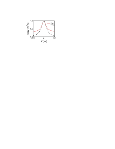
Supplementary Figure 1: The differential conductance ($dI/dV$) as a function of source voltage ($V$) at zero field.

In our experiment, as $k_{\rm B}T_{\rm K}=138\ {\rm\mu eV}$ and $\gamma_{0}=65\ {\rm\mu eV}$, $k_{\rm B}T_{\rm K}/\gamma_{0}\sim 2$ is the case. This is expected for $R\rightarrow 2$, which can be explained as follows. In the TRS and PHS case, the following is established OguriJPSJ2005 ,

$$\frac{dI}{dV}=\dfrac{2e^{2}}{h}\left[1-\frac{1+5(R-1)^{2}}{4}\left(\frac{eV}{\tilde{\Gamma}}\right)^{2}\right].$$ (25)

Here, $\tilde{\Gamma}$ is the renormalized width of the Kondo resonance, which depends on $U$ and $\Gamma$. For $U/\Gamma\rightarrow\infty$ ($R\rightarrow 2$), $\tilde{\Gamma}=4k_{\rm B}T_{\rm K}/\pi$ holds, and thus,

$$\frac{dI}{dV}=\frac{2e^{2}}{h}\left[1-\frac{3}{2}\left(\frac{\pi}{4}\right)^{2}\left(\frac{eV}{k_{\rm B}T_{\rm K}}\right)^{2}\right].$$ (26)

On the other hand, for $|eV/2\gamma_{0}|\ll 1$, Equation (22) yields

$$\frac{dI}{dV}=\dfrac{2e^{2}}{h}\dfrac{\gamma_{0}^{2}}{(eV/2)^{2}+\gamma_{0}^{2}}\rightarrow\frac{2e^{2}}{h}\left[1-\left(\frac{eV}{2\gamma_{0}}\right)^{2}\right].$$ (27)

Comparing these two, the following is obtained.

$$\frac{k_{\rm B}T_{\rm K}}{\gamma_{0}}=\sqrt{\frac{3}{8}}\pi=1.923\cdots.$$ (28)

It is interesting to note that, when $T_{\rm K}$ is given, the differential conductance tells us information on $R$ in this way.

SUPPLEMENTARY NOTE 2

The analysis in the Kondo regime

Magnetic field dependence of Kondo temperature

The solid curves in Supplementary Figure 2(a) are experimental conductance at different magnetic fields. We obtain $\gamma_{0}(B)$ and $G_{0}(B)$ for each field by fitting the experimental results with Supplementary Equation (12). Supplementary Figure 2(b) shows $\mu_{\rm B}B/k_{\rm B}T_{\rm K}$ or $B$ dependence of $\gamma_{0}(0)/\gamma_{0}(B)$ and $G_{0}(B)$. $T_{\rm K}$ is the Kondo temperature at zero field, which we evaluated from the temperature dependence (see the main text).

In the $U=0$ case, $T^{\ast}_{\rm K}(B)$, $\gamma_{0}(B)$, and phase shift $\delta_{\sigma}$ are related as:

$$4k_{\rm B}T^{\ast}_{\rm K}=\dfrac{\pi\gamma_{0}(B)}{\sin^{2}{\delta_{\sigma}}}.$$ (29)

Here, $T^{\ast}_{\rm K}$ is a characteristic temperature nominally obtained according to the definition of $T^{\ast}_{\rm K}\equiv 1/(4\sqrt{\chi_{\uparrow\uparrow}\chi_{\downarrow\downarrow}})$.

Thus, we obtain the following relation between $T^{\ast}_{\rm K}$ and $\gamma_{0}(B)$:

$$\dfrac{T_{\rm K}^{\ast}(0)}{T_{\rm K}^{\ast}(B)}=\dfrac{\gamma_{0}(0)}{\gamma_{0}(B)}\dfrac{G(B)}{G(0)},$$ (30)

Thus, we get $T_{\rm K}^{\ast}(0)/T_{\rm K}^{\ast}(B)$ by multiplying $\gamma_{0}(0)/\gamma_{0}(B)$ and $G_{0}(B)$ [the red circles in Supplementary Figure 2(c). The evaluation agrees well with the theoretical curve given by NRG calculations with $U/\Gamma=3.5$ OguriPRB2018_2 .

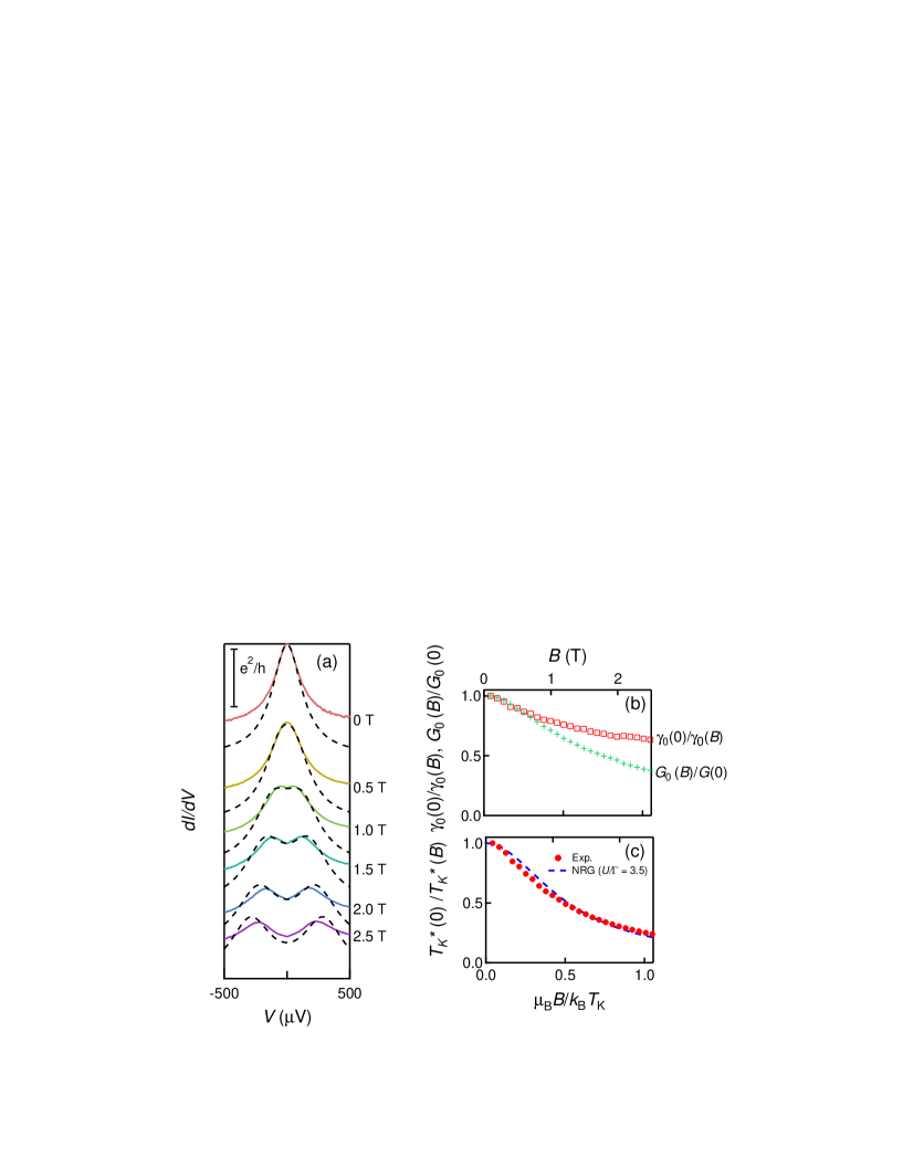
Supplementary Figure 2: (a) $dI/dV$ as a function of $V$ for different magnetic fields. The dashed lines are fitting curves with Supplementary Equation (12). (b) The red squares are $\gamma_{0}(0)/\gamma_{0}(B)$ obtained from the fitting. The green cross marks are the zero bias conductance. (c) The red circles are $T_{\rm K}^{\ast}(0)/T_{\rm K}^{\ast}(B)$, which we obtained by multiplying $\gamma_{0}(0)/\gamma_{0}(B)$ with $G(B)/G(0)$. The dashed line is given by the NRG calculations with $U/\Gamma=3.5$.

Small dip in conductance at finite magnetic field.

Supplementary Figure 3(a) is $dI/dV$ as a function of $eV/k_{\rm B}T_{\rm K}$ at $2\ \rm{T}$ ($\mu_{\rm B}B/k_{\rm B}T_{\rm K}=0.84$), where Zeeman splitting (ZS) is clearly seen. There is a small dip or cusp-like structure just around the zero bias, whose shape is not parabolic to cause a sharp change in $dI/dV$ as a function of ${\rm sign}(V)\times(eV/k_{\rm B}T_{\rm K})^{2}$ [Supplementary Figure 3(b)]. This may be attributed to the two-stage Kondo effect vanderWielPRL2002 and we do not use several points near zero bias to avoid this effect.

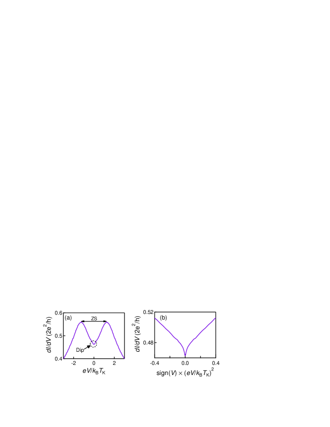
Supplementary Figure 3: (a) $dI/dV$ as a function of $eV/k_{\rm B}T_{\rm K}$ at $2\ {\rm T}$. The circle points out a very small dip or cusp-like structure just around the zero bias, which might be attributed to the two-stage Kondo effect. (b) $dI/dV$ as a function of ${\rm sign}(V)\times(eV/k_{\rm B}T_{\rm K})^{2}$ at $2\ {\rm T}$. The small dip in the left figure is attributed to the sharp slope around zero bias.

Magnetic field and gate voltage dependence of the Wilson ratio

Supplementary Figures 4 (a) and (b) are $\mu_{\rm B}B/k_{\rm B}T_{\rm K}$ and $\varepsilon/U$ dependence of $R-1$, which are given by the NRG calculations with $U/\Gamma=3.5$, respectively OguriPRB2018_2 . Here, $R$ is the Wilson ratio. The Wilson Ratio decreases as the time-reversal and particle-hole symmetry are broken. The insets are the expanded views of $R-1$ whose horizontal scale corresponds to those shown in the main text, showing the value does not change in these regions. Thus, we use experimental value of $R=1.95$ at zero field and at $\varepsilon=-U/2$ for our analysis.

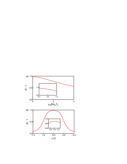
Supplementary Figure 4: (a) (b) $R-1$ as a function of $\mu_{\rm B}B/k_{\rm B}T_{\rm K}$ and $\varepsilon/U$, respectively, which are given by the NRG calculations with $U/\Gamma=3.5$ OguriPRB2018_2 .

SUPPLEMENTARY NOTE 3

Analysis procedure

We show the analysis procedures to obtain $W_{2}$ and $W_{3}$ as a function of magnetic field and gate voltage as follows.

Magnetic field dependence of $W_{2}$

1. We obtain $T_{\rm K}$ by analyzing the temperature dependence of $G_{0}$ FerrierNatPhys2016 .

2. We obtain $T_{\rm K}^{\ast}(\varepsilon=0,\ B)$ by analyzing $dI/dV$ at each field [Supplementary Note 2 and Supplementary Fig. 2(c)].

3. We derive $m_{d}(B)$ from $G_{0}(B)$ by using $G_{0}=\dfrac{2e^{2}}{h}\cos^{2}{(\pi m_{d})}$ (Fig. 3a in the main text).

4. We obtain $R=1.95$ at $B=0\ {\rm T}$ by the shot noise measurement FerrierNatPhys2016 .

5. We assume that $R$ is constant up to $\mu_{B}B/k_{\rm B}T_{\rm K}\sim 1$, which is justified by the NRG calculation [Supplementary Note 2 and Supplementary Fig. 4(a)].

6. We obtain $W_{2}$ as a function of $\mu_{\rm B}B/k_{\rm B}T_{\rm K}$ by using $W_{2}=-\left[1+5(R-1)^{2}\right]\cos{(\pi m_{d})}$ (Fig. 3a in the main text).

Magnetic field dependence of $W_{3}$

1. We plot $dI/dV$ as a function of ${\rm sign}(V)\times(eV/k_{\rm B}T_{\rm K})^{2}$, and obtain $\alpha_{\rm V}$ at each magnetic field by fitting the plotted points with $dI/dV=G_{0}-\alpha_{\rm V}(eV/k_{\rm B}T_{\rm K})^{2}$ (Fig. 3b in the main text).

2. We calculate $W_{3}$ by using $\alpha_{\rm V}$, $W_{2}$, $T_{\rm K}$, and $T_{\rm K}^{\ast}$ with Equation (6) in the main text (Fig. 3c in the main text).

Gate voltage dependence of $W_{2}$

1. We obtain $T_{\rm K}^{\ast}(\varepsilon,\ B=0)$ by analyzing the temperature dependence of $G_{0}$ at each gate voltage [Fig. 2a in the main text].

2. We derive $\delta_{\sigma}(\varepsilon)$ from $G_{0}(\varepsilon)$ by using $G_{0}=\dfrac{2e^{2}}{h}\sin^{2}{\delta_{\sigma}}$. Here, we assume that $\delta_{\sigma}=\delta_{\uparrow}=\delta_{\downarrow}$ and that $\delta_{\sigma}>\pi/2$ and $\delta_{\sigma}<\pi/2$ for $\varepsilon/U<-0.5$ and $\varepsilon/U>-0.5$, respectively [Fig. 4a in the main text].

3. We assume that $R$ is constant in a wide region $|\varepsilon/U+0.5|<0.15$, which is justified by the NRG calculation [Section C3 and Supplementary Figure 4(b)].

4. We obtain $W_{2}$ as a function of $\varepsilon/U$ by using $W_{2}=\left[1+5(R-1)^{2}\right]\cos{2\delta_{\sigma}}$ [Supplementary Figure 5].

Gate voltage dependence of $W_{3}$

1. We plot $dI/dV$ as a function of ${\rm sign}(V)\times(eV/k_{\rm B}T_{\rm K})^{2}$, and obtain $\alpha_{\rm V}$ at each gate voltage by fitting the plotted points with $dI/dV=G_{0}-\alpha_{\rm V}(eV/k_{\rm B}T_{\rm K})^{2}$ [Fig. 4b in the main text].

2. We obtain $W_{3}$ by using $W_{2}$, $T_{\rm K}$, $T_{\rm K}^{\ast}$, and Eq. (3) shown in the main text [Fig. 4c in the main text].

Supplementary Figure 5: $W_{2}$ as a function of $\varepsilon/U$. The points are experimental results, while the lines are theoretical ones.

SUPPLEMENTARY NOTE 4

Supplemental data

In this study, we measure the Kondo ridge at $N=3$ in the sample that has been used in Refs. FerrierNatPhys2016 ; FerrierPRL2017 ; Hata2018 , where $N$ is the number of electrons in the last shell. Supplementary Figure 6(b) is the color plot of $dI/dV$ as a function of $V$ and $V_{\rm g}$, where $V$ and $V_{\rm g}$ are source-drain voltage and gate voltage, respectively. Here, the magnetic field, $B=0.08\ {\rm T}$, is applied to suppress the superconductivity of the electrodes. The particle-hole symmetry point, $\varepsilon/U=-0.5$, is also indicated.

We also show $W_{2}$, $m_{d}$, $\alpha_{\rm V}$, and $W_{3}$ as a function of $B$ in Supplementary Figures 7(a)–(c). While the same data as a function of the normalized magnetic field $\mu_{\rm B}B/k_{\rm B}T_{\rm K}$ are shown in Figs. 3a, 3b, and 3c in the main text, these graphs shown as a function of $B$ itself might be useful for future analysis.

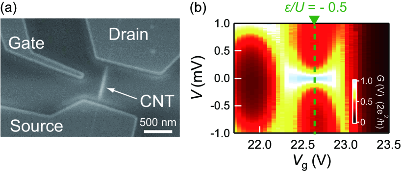
Supplementary Figure 6: (a) Scanning electron micrograph of a carbon nanotube quantum dot. (b) Color plot of $dI/dV$ as a function of $V$ and $V_{\rm g}$.

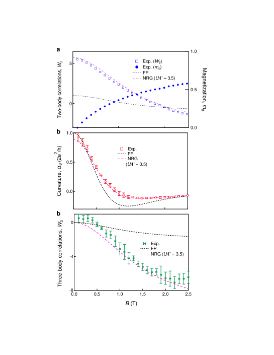
Supplementary Figure 7: (a) – (c) $W_{2}$, $m_{d}$, $\alpha_{\rm V}$, and $W_{3}$ as a function of magnetic field. The points are experimental results, while the lines are theoretical ones. The dotted and dashed lines for $W_{2}$ are given by the free particle (FP) model and the NRG calculations ($U/\Gamma=3.5$), respectively. Error bars in Supplementary Figure 7(b) correspond to the uncertainty of the linear fit performed on slightly different ranges. The error bars in Supplementary Figure 7(c) are determined based on those of $\alpha_{\rm V}$ shown in Supplementary Figure 7(b).

References

(1)
Oguri, A. & Hewson, A. C.
Higher-order Fermi-liquid corrections for an
Anderson impurity away from half filling.
Physical Review Letters120, 126802
(2018).
(2)
Nozieres, P.
A ”Fermi-liquid” description of the Kondo problem
at low temperatures.
Journal of Low Temperature Physics17, 31–42
(1974).
(3)
Yosida, K. & Yamada, K.
Perturbation expansion for the anderson hamiltonian.
Progress of Theoretical Physics Supplement46, 244–255
(1970).
(4)
Oguri, A.
Fermi liquid theory for the nonequilibrium Kondo
effect at low bias voltages.
Journal of the Physical Society of Japan74, 110–117
(2005).
(5)
Oguri, A. & Hewson, A. C.
Higher-order Fermi-liquid corrections for an
Anderson impurity away from half filling: Nonequilibrium transport.
Physical Review B97, 035435
(2018).
(6)
van der Wiel, W. G. et al.Two-stage Kondo effect in a quantum dot at a high
magnetic field.
Physical Review Letters88, 126803
(2002).
(7)
Ferrier, M. et al.Universality of non-equilibrium fluctuations in
strongly correlated quantum liquids.
Nature Physics12, 230–235
(2016).
(8)
Ferrier, M. et al.Quantum fluctuations along symmetry crossover in a
Kondo-correlated quantum dot.
Physical Review Letters118, 196803
(2017).
(9)
Hata, T. et al.Enhanced shot noise of multiple andreev reflections
in a carbon nanotube quantum dot in SU(2) and SU(4) kondo regimes.
Physical Review Letters121 (2018).