Informing Geometric Deep Learning with Electronic Interactions to Accelerate Quantum Chemistry
Abstract
Predicting electronic energies, densities, and related chemical properties can facilitate the discovery of novel catalysts, medicines, and battery materials. By developing a physics-inspired equivariant neural network, we introduce a method to learn molecular representations based on the electronic interactions among atomic orbitals. Our method, OrbNet-Equi, leverages efficient tight-binding simulations and learned mappings to recover high fidelity quantum chemical properties. OrbNet-Equi models a wide spectrum of target properties with an accuracy consistently better than standard machine learning methods and a speed several orders of magnitude greater than density functional theory. Despite only using training samples collected from readily available small-molecule libraries, OrbNet-Equi outperforms traditional methods on comprehensive downstream benchmarks that encompass diverse main-group chemical processes. Our method also describes interactions in challenging charge-transfer complexes and open-shell systems. We anticipate that the strategy presented here will help to expand opportunities for studies in chemistry and materials science, where the acquisition of experimental or reference training data is costly.
Discovering new molecules and materials is central to tackling contemporary challenges in energy storage and drug discovery [1, 2]. As the experimentally uninvestigated chemical space for these applications is immense, large-scale computational design and screening for new molecule candidates has the potential to vastly reduce the burden of laborious experiments and to accelerate discovery [3, 4, 5]. A crucial task is to model the quantum chemical properties of molecules by solving the many-body Schrödinger equation, which is commonly addressed by ab initio electronic structure methods [6, 7] such as density functional theory (DFT) (Figure 1a). While very successful, ab initio methods are laden with punitive computational requirements that makes it difficult to achieve a throughput on a scale of the unexplored chemical space.
In contrast, machine learning (ML) approaches are highly flexible as function approximators, and thus are promising for modelling molecular properties at a drastically reduced computational cost. A large class of ML-based molecular property predictors includes methods that use atomic-coordinate-based input features which closely resemble molecular mechanics (MM) descriptors [8, 9, 10, 11, 12, 13, 14, 15, 16, 17, 18]; these methods will be referred to as Atomistic ML methods in the current work (Figure 1b). Atomistic ML methods have been employed to solve challenging problems in molecular sciences such as RNA structure prediction [19] and anomalous phase transitions [20]. However, there remains a key discrepancy between Atomistic ML and ab initio approaches regarding the modelling of quantum chemical properties, as Atomistic ML approaches typically neglect the electronic degrees of freedom which are central for the description of important phenomena such as electronic excitations, charge transfer, and long-range interactions. Moreover, recent work shows that Atomistic ML can struggle with transferability on downstream tasks where the molecules may chemically deviate from the training samples [21, 22] as is expected to be common for under-explored chemical spaces.
Recent efforts to embody quantum mechanics (QM) into molecular representations based on electronic structure theory have made breakthroughs in improving both the chemical and electronic transferability of ML-based molecular modelling [23, 24, 25, 26, 27, 28, 29]. Leveraging a physical feature space extracted from QM simulations, such QM-informed ML methods have attained data efficiency that significantly surpass Atomistic ML methods, especially when extrapolated to systems with length scales or chemical compositions unseen during training. Nevertheless, QM-informed ML methods still fall short in terms of the flexibility of modelling diverse molecular properties unlike their atomistic counterparts, as they are typically implemented for a limited set of learning targets such as the electronic energy or the exchange-correlation potential. A key bottleneck hampering the broader applicability of QM-informed approaches is the presence of unique many-body symmetries necessitated by an explicit treatment on electron-electron interactions. Heuristic schemes have been used to enforce invariance [30, 31, 24, 26, 32, 33] at a potential loss of information in their input features or expressivity in their ML models. Two objectives remain elusive for QM-informed machine learning: (a) incorporate the underlying physical symmetries with maximal data efficiency and model flexibility, and (b) accurately infer downstream molecular properties for large chemical spaces, at a computational resource requirement on par with existing empirical and Atomisic ML methods.
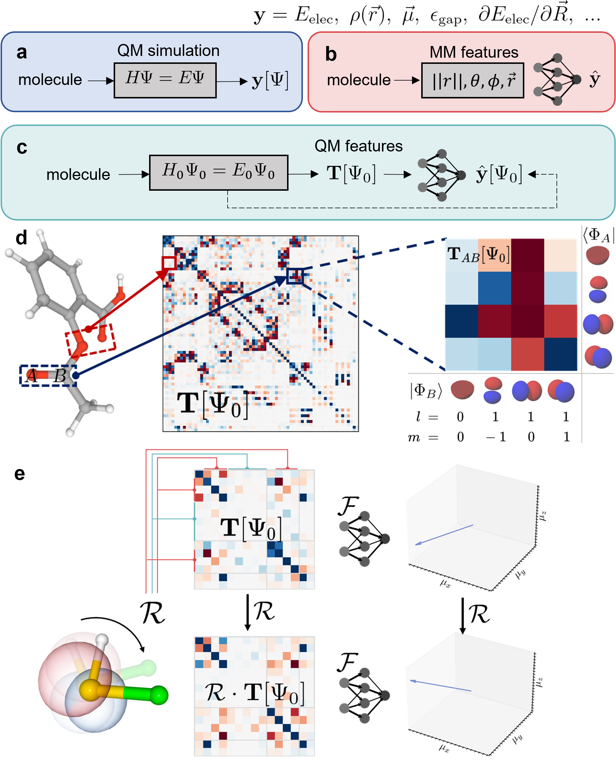
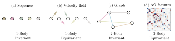
Herein, we introduce an end-to-end ML method for QM-informed molecular representations, OrbNet-Equi, in fulfillment of these two objectives. OrbNet-Equi featurizes a mean-field electronic structure via the atomic orbital basis, and learns molecular representations through a machine learning model that is equivariant with respect to isometric basis transformations (Figure 1c-e). By the virtue of equivariance, OrbNet-Equi respects essential physical constraints of symmetry conservation so that the target quantum chemistry properties are learned independent of a reference frame. Underpinning OrbNet-Equi is a neural network designed with insights from recent advances in geometric deep learning [34, 35, 36, 37, 38, 39, 40], but with key architectural innovations to achieve equivariance based on the tensor-space algebraic structures entailed in atomic-orbital-based molecular representations.
We demonstrate the data efficiency of OrbNet-Equi on learning molecular properties using input features obtained from tight-binding QM simulations which are efficient and scalable to systems with thousands of atoms [41]. We find that OrbNet-Equi consistently achieves lower prediction errors than existing Atomistic ML methods and our previous QM-informed ML method [26] on diverse target properties such as electronic energies, dipole moments, electron densities, and frontier orbital energies. Specifically, our study on learning frontier orbital energies illustrates an effective strategy to improve the prediction of electronic properties by incorporating molecular-orbital-space information.
To showcase its transferability to complex real-world chemical spaces, we trained an OrbNet-Equi model on single-point energies of 236k molecules curated from readily available small-molecule libraries. The resulting model, OrbNet-Equi/SDC21, achieves a performance competitive to state-of-the-art composite DFT methods when tested on a wide variety of main-group quantum chemistry benchmarks, while being up to thousand-fold faster at runtime. As a particular case study, we found that OrbNet-Equi/SDC21 substantially improved the prediction accuracy of ionization potentials relative to semi-empirical QM methods, even though no radical species was included for training. Thus, our method has the potential to accelerate simulations for challenging problems in organic synthesis [42], battery design [43], and molecular biology [44]. Detailed data analysis pinpoints viable future directions to systematically improve its chemical space coverage, opening a plausible pathway towards a generic hybrid physics-ML paradigm for the acceleration of molecular modelling and discovery.
Results
The OrbNet-Equi methodology
OrbNet-Equi featurizes a molecular system through mean-field QM simulations. Semi-empirical tight-binding models [41] are used through this study since they can be solved rapidly for both small-molecules and extended systems, which enables deploying OrbNet-Equi to large chemical spaces. In particular, we employ the recently reported GFN-xTB [45] QM model in which the mean-field electronic structure is obtained through self-consistently solving a tight-binding model system (Figure 1c). Built upon , the inputs to the neural network comprises a stack of matrices defined as single-electron operators represented in the atomic orbitals (Figure 1d),
| (1) |
where and are both atom indices; and indicate a basis function in the set of atomic orbitals centered at each atom. Motivated by mean-field electronic energy expressions, the input atomic orbital features are selected as using the Fock , density , core-Hamiltonian , and overlap matrices of the tight-binding QM model (see Methods 1.2), unless otherwise specified.
OrbNet-Equi learns a map to approximate the target molecular property of high-fidelity electronic structure simulations or experimental measurements,
| (2) |
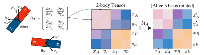
where denotes a cost functional between the reference and predicted targets over training data. The learning problem described by (2) requires a careful treatment on isometric coordinate transformations imposed on the molecular system, because the coefficients of are defined up to a given viewpoint (Figure 1e). Precisely, the atomic orbitals undergo a unitary linear recombination subject to 3D rotations: , where denotes the Wigner-D matrix of degree for a rotation operation . As a consequence of the basis changing induced by , is transformed block-wise:
| (3) |
where the dagger symbol denotes an Hermitian conjugate. To account for the roto-translation symmetries, the neural network must be made equivariant with respect to all such isometric basis rotations, that is,
| (4) |
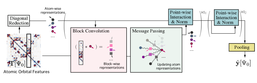
which is fulfilled through our delicate design of the neural network in OrbNet-Equi (Figure 2). The neural network iteratively updates a set of representations defined at each atom through its neural network modules, and reads out predictions using a pooling layer located at the end of the network. During its forward pass, diagonal blocks of the inputs are first transformed into components that are isomorphic to orbital-angular-momentum eigenstates, which are then cast to the initial representations . Each subsequent module exploits off-diagonal blocks of to propagate non-local information among atomic orbitals and refine the representations , which resembles a process of applying time-evolution operators on quantum states. We provide a technical introduction to the neural network architecture in Methods 1.1. We incorporate other constraints on the learning task such as size-consistency solely through programming the pooling layer (Methods S1.5), therefore achieving task-agnostic modelling for diverse chemical properties. Additional details and theoretical results are provided in Appendix S1-S2.
Performance on benchmark datasets
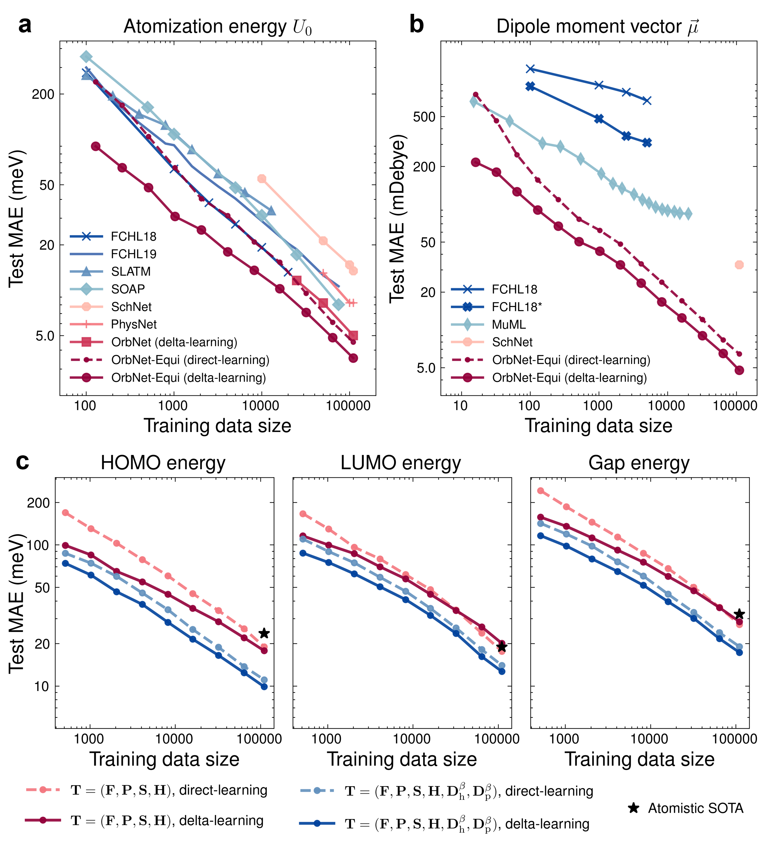
We begin with benchmarking OrbNet-Equi on the QM9 dataset [46] which has been widely adopted for assessing ML-based molecular property prediction methods. QM9 contains 134k small organic molecules at optimized geometries, with target properties computed by DFT. Following previous works [13, 14, 38, 47, 18, 17], we take 110000 random samples as the training set and 10831 samples as the test set. We present results for both the “direct-learning” training strategy which corresponds to training the model directly on the target property, and, whenever applicable, the “delta-learning” strategy [48] which corresponds to training on the residual between output of the tight-binding QM model and the target level of theory.
We first trained OrbNet-Equi on two representative targets, the total electronic energy and the molecular dipole moment vector (Figure 3a-b), for which a plethora of task-specific ML models has previously been developed [49, 50, 51, 26, 52, 53]. The total energy is predicted through a sum over atom-wise energy contributions and the dipole moment is predicted through a combination of atomic partial charges and dipoles (Appendix S1.5). For (Figure 3a), the direct-learning results of OrbNet-Equi match the state-of-the-art kernel-based ML method FCHL18/GPR [50] in terms of the test mean absolute error (MAE), while being scalable to large data regimes (Figure 3a, training data size > 20,000) where no competitive result has been reported before. With delta-learning, OrbNet-Equi outperforms our previous QM-informed ML approach OrbNet [26] by in the test MAE. Because OrbNet also uses the GFN-xTB QM model for featurization and the delta-learning strategy for training, this improvement underscores the strength of our neural network design which seamlessly integrates the underlying physical symmetries. Moreover, for dipole moments (Figure 3b), OrbNet-Equi exhibits steep learning curve slopes regardless of the training strategy, highlighting its capability of learning rotational-covariant quantities at no sacrifice of data efficiency.
We then targeted on the learning task of frontier molecular orbital (FMO) properties, in particular energies of the highest occupied molecular orbital (HOMO), the lowest unoccupied molecular orbital (LUMO) and the HOMO-LUMO gaps which are important in the prediction of chemical reactivity and optical properties [54, 55]. Because the FMOs are inherently defined in the electron energy space and are often spatially localized, it is expected to be challenging to predict FMO properties based on molecular representations in which a notion of electronic energy levels is absent. OrbNet-Equi overcame this obstacle by breaking the orbital filling degeneracy of its input features to encode plausible electron excitations near the FMO energy levels, that is, adding energy-weighted density matrices of ‘hole-excitation’ and that of ‘particle-excitation’ :
| (5) | ||||
| (6) |
where and are the orbital energy and occupation number of the -th molecular orbital from tight-binding QM, and denotes the molecular orbital coefficients with and indexing the atomic orbital basis. Here the effective temperature parameters are chosen as (atomic units), and a global-attention based pooling is used to ensure size-intensive predictions (Appendix S1.5.4). Figure 3c shows that the inclusion of energy-weighted density matrices () indeed greatly enhanced model generalization on FMO energies, as evident from the drastic test MAE reduction against the model with default ground-state features () as well as the best result from Atomistic ML methods. Remarkably, for models using default ground-state features (Figure 3c, red lines) we noticed a rank reversal behavior between direct-learning and delta-learning models as more training samples become available, mirroring similar observations from a recent Atomistic ML study [56]. The absence of this crossover when () are provided (Figure 3c, blue) suggests that the origin of such a learning slow-down is the incompleteness of spatially-degenerate descriptors, and the gap between delta-learning and direct-learning curves can be restored by breaking the energy-space degeneracy. This analysis reaffirms the role of identifying the dominant physical degrees of freedom in the context of ML-based prediction of quantum chemical properties, and is expected to benefit the modelling of relevant electrochemical and optical properties such as redox potentials.
Furthermore, OrbNet-Equi is benchmarked on 12 targets of QM9 using the 110k full training set (Appendix Table S1), for which we programmed its pooling layer to reflect the symmetry constraint of each target property (Appendix S1.5). We observed top-ranked performance on all targets with average test MAE around two-fold lower than atomistic deep learning methods. In addition, we tested OrbNet-Equi on fitting molecular potential energy surfaces by training on multiple configurations of a molecule (Appendix S3.2). Results (Appendix Table S2-S3) showed that OrbNet-Equi obtained energy and force prediction errors that match state-of-the-art machine learning potential methods [57, 58] on the MD17 dataset [59, 57], suggesting that our method also efficiently generalizes over the conformation degrees of freedom apart from being transferable across the chemical space. These extensive benchmarking studies confirm that our strategy is consistently applicable to a wide range of molecular properties.
Accurate modelling for electron densities
We next focus on the task of predicting the electron density which plays an essential role in both the formulation of DFT and in the interpretation of molecular interactions. It is also more challenging than predicting the energetic properties from a machine learning perspective, due to the need of preserving its real-space continuity and rotational covariance. OrbNet-Equi learns to output a set of expansion coefficients to represent the predicted electron density through a density fitting basis set (Methods 1.3, Appendix S1.5.6),
| (7) |
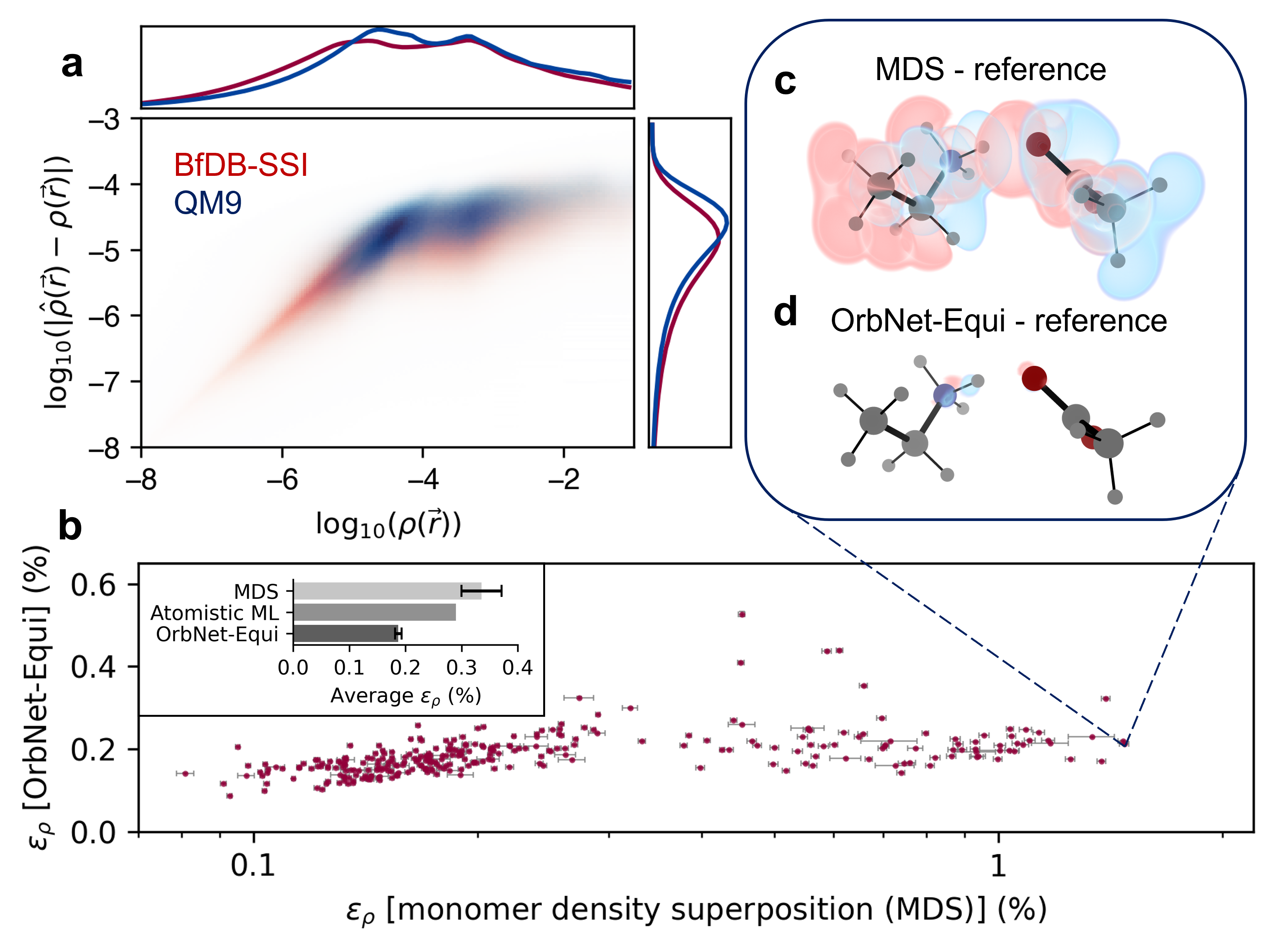
where is the maximum angular momentum in the density fitting basis set for atom type , and denotes the cardinality of basis functions with angular momentum . We train OrbNet-Equi to learn DFT electron densities on the QM9 dataset of small organic molecules and the BfDB-SSI [60] dataset of amino-acid side-chain dimers (Figure 4) using the direct-learning strategy. OrbNet-Equi results are substantially better than Atomistic ML baselines in terms of the average density error (Methods 1.3); specifically, OrbNet-Equi achieves an average of 0.1910.003% on BfDB-SSI using 2000 training samples compared to 0.29% of SA-GPR [61], and an average of 0.2060.001% on QM9 using 123835 training samples as compared to 0.28%-0.36% of DeepDFT [62]. Figure 4a confirms that OrbNet-Equi predicts densities at consistently low errors across the real-space and maintains a robust asymptotic decay behavior within low-density () regions that are far from the molecular system.
To understand whether the model generalizes to cases where charge transfer is significant, as in donor-acceptor systems, we introduce a simple baseline predictor termed monomer density superposition (MDS). The MDS electron density of a dimeric system is taken as the sum of independently-computed DFT electron densities of the two monomers. OrbNet-Equi yields accurate predictions in the presence of charge redistribution induced by non-covalent effects, as identified by dimeric examples from the BfDB-SSI test set for which the MDS density (Figure 4b, x-axis) largely deviates from the DFT reference density of the dimer due to inter-molecular interactions. One representative example is a strongly interacting Glutamic acid - Lysine system (Figure 4, c-d) whose salt-bridge formation is known to be essential for the helical stabilization in protein folding [63], for which OrbNet-Equi predicts with significantly lower than that of monomer density superposition (). The accurate modelling of offers an opportunity for constructing transferable DFT models for extended systems by learning on both energetics and densities, while at a small fraction of expense relative to solving the Kohn-Sham equations from scratch.
Transferability on downstream tasks
Beyond data efficiency on established datasets in train-test split settings, a crucial but highly challenging aspect is whether the model accurately infers downstream properties after being trained on data that are feasible to obtain. To comprehensively evaluate whether OrbNet-Equi can be transferred to unseen chemical spaces without any additional supervision, we have trained an OrbNet-Equi model on a dataset curated from readily available small-molecule databases (Methods 1.3). The training dataset contains 236k samples with chemical space coverage for drug-like molecules and biological motifs containing chemical elements C, O, N, F, S, Cl, Br, I, P, Si, B, Na, K, Li, Ca and Mg, and thermalized geometries. The resulting OrbNet-Equi/SDC21 potential energy model is solely trained on DFT single-point energies using the delta-learning strategy. Without any fine-tuning, we directly apply OrbNet-Equi/SDC21 to downstream benchmarks that are recognized for assessing the accuracy of physics-based molecular modelling methods.
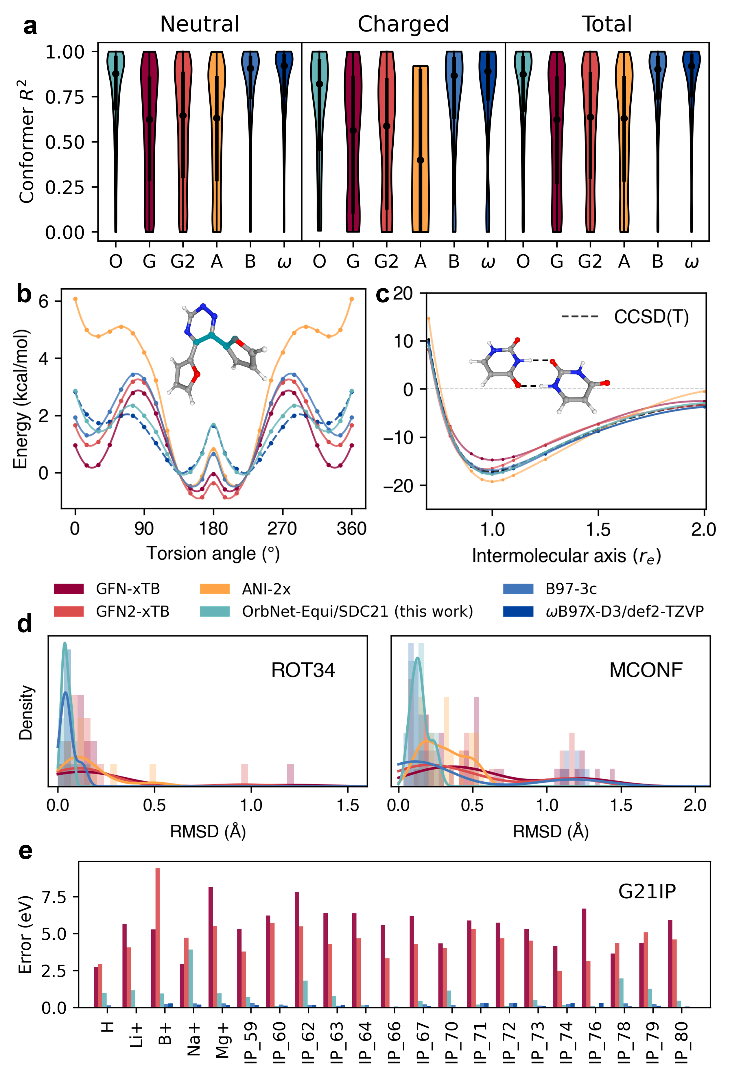
The task of ranking conformer energies of drug-like molecules is benchmarked via the Hutchison dataset of conformers of 700 molecules [21] (Figure 5a; Table S5, row 1-2). On this task, OrbNet-Equi/SDC21 achieves a median score of 0.87±0.02 and distributions closely matching the reference DFT theory on both neutral and charged systems. On the other hand, we notice that the median of OrbNet-Equi/SDC21 with respect to the reference DFT theory (B97X-D3/def2-TZVP) is 0.96±0.01, suggesting that the current performance on this task is saturated by the accuracy of DFT and can be systematically improved by applying fine-tuning techniques on higher-fidelity labels [64, 65]. Timing results on the Hutchison dataset (Table S4) confirms that the neural network inference time of OrbNet-Equi/SDC21 is on par with the GFN-xTB QM featurizer, resulting in an overall computational speed that is fold faster relative to existing cost-efficient composite DFT methods [21, 66, 67]. To understand the model’s ability to describe dihedral energetics which are crucial for virtual screening tasks, we benchmark OrbNet-Equi on the prediction of intra-molecular torsion energy profiles using the TorsionNet500 [68] dataset, the most diverse benchmark set available for this problem (Table S5, row 3). Although no explicit torsion angle sampling was performed during training data generation, OrbNet-Equi/SDC21 exhibits a barrier MAE of 0.1730.003 kcal/mol much lower than the 1 kcal/mol threshold commonly considered for chemical accuracy. On the other hand, we notice a MAE of 0.7 kcal/mol for the TorsionNet model [68] which was trained on 1 million torsion energy samples. As shown in Figure 5b, OrbNet-Equi/SDC21 robustly captures the torsion sectors of potential energy surface on an example challenging for both semi-empirical QM [45, 69] and cost-efficient composite DFT [66] methods, precisely resolving both the sub-optimal energy minima location at dihedral angle as well as the barrier energy between two local minimas within a 1 kcal/mol chemical accuracy. Next, the ability to characterize non-covalent interactions is assessed on the S66x10 dataset [70] of inter-molecular dissociation curves (Table S6), on which OrbNet-Equi achieves an equilibrium-distance binding energy MAE of kcal/mol with respect to the reference DFT theory compared against kcal/mol of the GFN-xTB baseline. As shown from a Uracil-Uracil base-pair example (Figure 5c) for which high-fidelity wavefunction-based reference calculations have been reported, the binding energy curve along the inter-molecular axis predicted by OrbNet-Equi/SDC21 agrees well with both DFT and the high-level CCSD(T) results. To further understand the accuracy and smoothness of the energy surfaces and the applicability on dynamics tasks, we perform geometry optimizations on the ROT34 dataset of 12 small organic molecules and the MCONF dataset of 52 conformers of melatonin [71, 72] (Figure 5d; Table S5, row 4-5). Remarkably, OrbNet-Equi/SDC21 consistently exhibits the lowest average RMSD among all physics-based and ML-based approaches (Table S5) including the popular cost-efficient DFT method B97-3c [66]. Further details regarding the numerical experiments and error metrics are provided in Methods 1.3.
Remarkably, on the G21IP dataset [73] of adiabatic ionization potentials, we find that the OrbNet-Equi/SDC21 model achieves prediction errors substantially lower than semi-empirical QM methods (Figure 5e, Table S7) even though samples of open-shell signatures are expected to be rare from the training set (Methods 1.3). Such an improvement cannot be solely attributed to structure-based corrections, since there is no or negligible geometrical changes between the neutral and ionized species for both the single-atom systems and several poly-atomic systems (e.g., IP_66, a Phosphanide anion) in the G21IP dataset. This reveals that our method has the potential to be transferred to unseen electronic states in a zero-shot manner, which represents an early evidence that a hybrid physics-ML strategy may unravel novel chemical processes such as unknown electron-catalyzed reactions [74].
To comprehensively study the transferability of OrbNet-Equi on complex under-explored main-group chemical spaces, we evaluate OrbNet-Equi/SDC21 on the challenging, community-recognized benchmark collection of the General Thermochemistry, Kinetics, and Non-covalent Interactions (GMTKN55)[75] datasets (Figure 6). Prediction error statistics on the GMTKN55 benchmark are reported with three filtration schemes. First, we evaluate the WTMAD error metrics (Methods 1.3) on reactions that only consist of neutral and closed-shell molecules with chemical elements CHONFSCl (Figure 6a), as is supported by an Atomistic-ML-based potential method, ANI-2x [76], which is trained on large-scale DFT data. OrbNet-Equi/SDC21 predictions are found to be highly accurate on this subset, as seen from the WTMAD with respect to CCSD(T) being on par with the DFT methods on all five reaction classes and significantly outperforming ANI-2x and the GFN family of semi-empirical QM methods [45, 69]. It is worth noting that OrbNet-Equi/SDC21 uses much fewer number of training samples than the ANI-2x training set, which signifies the effectiveness of combining physics-based and ML-based modelling.
The second filtration scheme includes reactions that consist of closed-shell - but can be charged - molecules with chemical elements that have appeared in the SDC21 training dataset (Figure 6b). Although all chemical elements and electronic configurations in this subset are contained in the training dataset, we note that unseen types of physical interactions or bonding types are included, such as in alkali metal clusters from the ALK8 subset [75] and short strong hydrogen bonds in the AHB21 subset [77]. Therefore, assessments of OrbNet-Equi with this filtration strategy reflect its performance on cases where examples of atom-level physics are provided but the the chemical compositions are largely unknown. Despite this fact, the median WTMADs of OrbNet-Equi/SDC21 are still competitive to DFT methods on the tasks of small-system properties, large-system properties and intra-molecular interactions. On reaction barriers and inter-molecular non-covalent interactions (NCIs), OrbNet-Equi/SDC21 results fall behind DFT but still show improvements against the GFN-xTB baseline and match the accuracy of GFN2-xTB which is developed with physic-based schemes to improve the descriptions on NCI properties against its predecessor GFN-xTB.
The last scheme includes all reactions in the GMTKN55 benchmarks containing chemical elements and spin states never seen during training (Figure 6c), which represents on the most stringent test and reflects the performance of OrbNet-Equi/SDC21 when being indiscriminately deployed as a quantum chemistry method. When evaluated on the collection of all GMTKN55 tasks (Figure 6, ‘Total’ panel), OrbNet-Equi/SDC21 maintains the lowest median WTMAD among methods considered here that can be executed at the computational cost of semi-empirical QM calculations. Moreover, we note that failure modes on a few highly extrapolative subsets can be identified to diagnose cases that are challenging for the QM model used for featurization (Table S7). For example, the fact that predictions being inaccurate on the W4-11 subset of atomization energies [78] and the G21EA subset of electron affinities [73] parallels the absence of an explicit treatment of triplet or higher-spin species within the formulation of GFN family of tight-binding models. On the population level, the distribution of prediction WTMADs across GMTKN55 tasks also differ from that of GFN2-xTB, which implies that further incorporating physics-based approximations into the QM featurizer can complement the ML model, and thus the accuracy boundary of semi-empirical methods can be pushed to a regime where no known physical approximation is feasible.
Discussion
We have introduced OrbNet-Equi, a QM-informed geometric deep learning framework for learning molecular or material properties using representations in the atomic orbital basis. OrbNet-Equi shows excellent data efficiency for learning related to both energy-space and real-space properties, expanding the diversity of molecular properties that can be modelled by QM-informed machine learning. Despite only using readily available small-molecule libraries as training data, OrbNet-Equi offers an accuracy alternative to DFT methods on comprehensive main-group quantum chemistry benchmarks at a computation speed on par with semi-empirical methods, thus offering a possible replacement for conventional ab initio simulations for general-purpose downstream applications. For example, OrbNet-Equi could immediately facilitate applications such as screening electrochemical properties of electrolytes for the design of flow batteries [43], and performing accurate direct or hybrid QM/MM simulations for reactions in transition-metal catalysis [42, 79]. The method can also improve the modelling for complex reactive biochemical processes [80] using multi-scale strategies that have been demonstrated in our previous study [44], while conventional ab initio reference calculations can be prohibitively expensive even on a minimal sub-system.
The demonstrated transferability of OrbNet-Equi to seemingly dissimilar chemical species identifies a promising future direction of improving the accuracy and chemical space coverage through adding simple model systems of the absent types of physical interactions to the training data, a strategy that is consistent with using synthetic data to improve ML models [81] which has been demonstrated for improving the accuracy of DFT functionals [29]. Additionally, OrbNet-Equi may provide valuable perspectives for the development of physics-based QM models by relieving the burden of parameterizing Hamiltonian parameters against specific target systems, potentially expanding their design space to higher energy-scales without sacrificing model accuracy. Because the framework presented here can be readily extended to alternative quantum chemistry models for either molecular or material systems, we expect OrbNet-Equi to broadly benefit studies in chemistry, materials science, and biotechnology.
1 Methods
1.1 The UNiTE neural network
This section introduces Unitary N-body Tensor Equivariant Network (UNiTE), the neural network model developed for the OrbNet-Equi method to enable learning equivariant maps between the input atomic orbital features and the property predictions . Given the inputs , UNiTE first generates initial representations through its diagonal reduction module (Methods 1.1.1). Then UNiTE updates the representations with stacks of block convolution (Methods 1.1.2), message passing (Methods 1.1.3), and point-wise interaction (Methods 1.1.5) modules, followed by stacks of point-wise interaction modules. A pooling layer (Methods 1.1.6) outputs predictions using the final representations at as inputs.
is a stack of atom-wise representations, i.e., for a molecular system containing atoms, . The representation for the -th atom, , is a concatenation of neurons which are associated with irreducible representations of group . Each neuron in is identified by a channel index , a "degree" index , and a "parity" index . The neuron is a vector of length and transforms as the -th irreducible representation of group ; i.e., where denotes a vector concatenation operation and . We use to denote the number of neurons with degree and parity in , and to denote the total number of neurons in .
For a molecular/material system with atomic coordinates , the following equivariance properties with respect to isometric Euclidean transformations are fulfilled for any input gauge-invariant and Hermitian operator ; for all allowed indices :
-
•
Translation invariance:
(8) where is an arbitrary global shift vector;
-
•
Rotation equivariance:
(9) for where denotes a rotation matrix corresponding to standard Euler angles ;
-
•
Parity inversion equivariance:
(10)
The initial vector representations are generated by decomposing diagonal sub-tensors of the input into a spherical-tensor representation without explicitly solving tensor factorization, based on the tensor product property of group . The intuition behind this operation is that the diagonal sub-tensors of can be viewed as isolated systems interacting with an effective external field, whose rotational symmetries are described by the Wigner-Eckart Theorem [82] which links tensor operators to their spherical counterparts and applies here within a natural generalization. Each update step is composed of (a) block convolution, (b) message passing, and (c) point-wise interaction modules which are all equivariant with respect to index permutations and basis transformations. In an update step , each off-diagonal block of corresponding to a pair of atoms is contracted with . This block-wise contraction operation can be interpreted as performing local convolutions using the blocks of as convolution kernels, and therefore is called block convolution module. The output block-wise representations are then passed into a message passing module, which is analogous to a message-passing operation on edges in graph neural networks [83]. The message passing outputs are then fed into a point-wise interaction module with the previous-step representation to finish the update . The point-wise interaction modules are constructed as a stack of multi-layer perceptrons (MLPs), Clebsch-Gordan product operations and skip connections. Within those modules, a matching layer assigns the channel indices of to indices of the atomic orbital basis.
We also introduce a normalization layer termed Equivariant Normalization (EvNorm, see Methods 1.1.4) to improve training and generalization of the neural network. EvNorm normalizes scales of the representations , while recording the direction-like information to be recovered afterward. EvNorm is fused with a point-wise interaction module through first applying EvNorm to the module inputs, then using an MLP to transform the normalized frame-invariant scale information, and finally by multiplying the recorded direction vector to the MLP’s output. Using EvNorm within the point-wise interaction modules is found to stabilize training and eliminate the need for tuning weight initializations and learning rates across different tasks.
The explicit expressions for the neural network modules are provided for quantum operators being one-electron operators and therefore the input tensors is a stack of matrices (i.e., order-2 tensors). Without loss of generality, we also assume that contains only one feature matrix. Additional technical aspects regarding the case of multiple input features, the inclusion of geometric descriptors, and implementation details are discussed in Appendix S1. The proofs regarding equivariance and theoretical generalizations to order- tensors are provided in Appendix S2.
1.1.1 The Diagonal Reduction module
We define the shorthand notations and to index atomic orbitals. The initialization scheme for is based on the following proposition: for each diagonal block of , , defined for an on-site atom pair ,
| (11) |
there exists a set of -independent coefficients such that the following linear transformation
| (12) |
is injective and yields that satisfy equivariance ((8)-(10)).
The existence of is discussed in Appendix, Corollary S3. For the sake of computational feasibility, a physically-motivated scheme is employed to tabulate and produce order-1 equivariant embeddings , using on-site 3-index overlap integrals :
| (13) |
where are the atomic orbital basis, and are auxiliary Gaussian-type basis functions defined as (for conciseness, at ):
| (14) |
where is a normalization constant such that following standard conventions [84]. For numerical experiments considered in this work the scale parameters are chosen as (in atomic units):
adheres to equivariance constraints due to its relation to Clebsch-Gordan coefficients [82]. Note that the auxiliary basis is independent of the atomic numbers thus the resulting are of equal length for all chemical elements. can be efficiently generated using electronic structure programs, here done with [85]. The resulting in explicit form are
are then projected by learnable linear weight matrices such that the number of channels for each matches the model specifications. The outputs are regarded as the initial representations to be passed into other modules.
1.1.2 The Block Convolution module
In an update step , sub-blocks of are first contracted with a stack of linearly-transformed order-1 representations .
| (15) |
which can be viewed as a 1D convolution between each block (as convolution kernels) and the (as the signal) in the -th channel where is the convolution channel index. The block convolution produces block-wise representations for each block index . is called a matching layer at atom and channel , defined as:
| (16) |
are learnable linear weight matrices specific to each degree index , where is the maximum principle quantum number for shells of angular momentum within the atomic orbital basis used for featurization. The operation maps the feature dimension to valid atomic orbitals by indexing using , the principle quantum numbers of atomic orbitals for atom type .
1.1.3 The Message Passing module
Block-wise representations are then aggregated into each atom index by summing over the indices , analogous to a ‘message-passing’ between nodes and edges in common realizations of graph neural networks [83],
| (17) |
up to a non-essential symmetrization and inclusion of point-cloud geometrical terms ((S5)). in (17) are scalar-valued weights parameterized as SE(3)-invariant multi-head attentions:
| (18) |
where denotes an element-wise (Hadamard) product, and
| (19) |
where denotes a 2-layer MLP, are learnable linear functions and denotes an attention head (one value in ). is chosen as Morlet wavelet basis functions:
| (20) | ||||
| (21) |
where are learnable linear functions and are learnable frequency coefficients initialized as where . Similar to the scheme proposed in -transformers [40], the attention mechanism (18) improves the network capacity without increasing memory costs as opposed to explicitly expanding .
The aggregated message is combined with the representation of current step through a point-wise interaction module (see Methods 1.1.5) to complete the update .
1.1.4 Equivariant Normalization (EvNorm)
We define where and are given by
| (22) |
where denotes taking a neuron-wise regularized norm:
| (23) |
and are mean and variance estimates of the invariant content that can be obtained from either batch or layer statistics as in normalization schemes developed for scalar neural networks [86, 87]; are positive, learnable scalars controlling the fraction of vector scale information from to be retained in , and is a numerical stability factor. The EvNorm operation (22) decouples to the normalized frame-invariant representation suitable for being transformed by an MLP, and a ‘pure-direction’ that is later multiplied to the MLP-transformed normalized invariant content to finish updating . Note that in (22), is always a fixed point of the map and the vector directions information is always preserved.
1.1.5 The Point-wise Interaction module and representation updates
A point-wise interaction module ((24)-(26)) nonlinearly updates the atom-wise representations through
| (24) | ||||
| (25) | ||||
| (26) |
which consist of coupling another -equivariant representation with and performing normalizations. In (24)-(26), are Clebsch-Gordan coefficients of group , is a Kronecker delta function, and and denote multi-layer perceptrons acting on the feature () dimension. and correspond to learnable linear weight matrices specific to the update step and each .
For , the updates are performed by combining with the aggregated messages from step :
| (27) |
where is called a reverse matching layer, defined as:
| (28) | ||||
| (29) |
the operation maps the atomic-orbital dimension in to a feature dimension with fixed length using as the indices, and flattens the outputs into shape . are learnable linear weight matrices to project the outputs into the shape of .
For , the updates are based on local information:
| (30) |
1.1.6 Pooling layers and training
A programmed pooling layer reads out the target prediction after the representations are updated to the last step . Pooling operations employed for obtaining main numerical results are detailed in Appendix S1.5; hyperparameter, training and loss function details are provided in Appendix S4. As a concrete example, the dipole moment vector is predicted as where is the 3D coordinate of atom , and atomic charges and atomic dipoles are predicted respectively using scalar () and Cartesian-coordinate vector () components of .
1.2 QM-informed featurization details and gradient calculations
The QM-informed representation employed in this work is motivated by a pair of our previous works [26, 88], but in this study the features are directly evaluated in the atomic orbital basis without the need of heuristic post-processing algorithms to enforce rotational invariance.
In particular, this work (as well as [26] and [88]) constructs features based on the GFN-xTB semi-empirical QM method [45]. As a member of the class of mean field quantum chemical methods, GFN-xTB centers around the self-consistent solution of the Roothaan-Hall equations,
| (31) |
All boldface symbols are matrices represented in the atomic orbital basis. For the particular case of GFN-xTB, the atomic orbital basis is similar to STO-6G and comprises a set of hydrogen-like orbitals. is the molecular orbital coefficients which defines , and is a diagonal eigenvalue matrix of the molecular orbital energies. is the overlap matrix and is given by
| (32) |
where and index the atomic orbital basis . is the Fock matrix and is given by
| (33) |
is the one-electron integrals including electron-nuclear attraction and electron kinetic energy. is the two-electron integrals comprising the electron-electron repulsion. Approximation of is the key task for self-consistent field methods, and GFN-xTB provides an accurate and efficient tight-binding approximation for . Finally, is the (one-electron-reduced) density matrix, and is given by
| (34) |
is the number of electrons, and a closed-shell singlet ground state is assumed for simplicity. Equations 31 and 33 are solved for . The electronic energy is related to the Fock matrix by
| (35) |
The particular form of the GFN-xTB electronic energy can be found in [45].
UNiTE is trained to predict the quantum chemistry properties of interest based on the inputs , , , with possible extensions (e.g., the energy-weighted density matrices). For the example of learning the DFT electronic energy with the "delta-learning" training strategy:
| (36) |
Note that , , , and all implicitly depend on the atomic coordinates and charge/spin state specifications.
In addition to predicting it is also common to compute its gradient with respect to atomic nuclear coordinates to predict the forces used for geometry optimization and molecular dynamics simulations. We directly differentiate the energy (36) to obtain energy-conserving forces. The partial derivatives of the UNiTE energy with respect to , , , and is determined through automatic differentiation. The resulting forces are computed through an adjoint approach developed in Appendix D of our previous work [88], with the simplification that the SAAO transformation matrix is replaced by the identity.
1.3 Dataset and computational details
Training datasets
The molecule datasets used in Section Performance on benchmark datasets-Accurate modelling for electron densities are all previously published. Following Section 2.1 of [61], the 2291 BFDb-SSI samples for training and testing are selected as the sidechain–sidechain dimers in the original BFDb-SSI dataset that contain 25 atoms and no sulfur element to allow for comparisons among methods.
The Selected Drug-like and biofragment Conformers (SDC21) dataset used for training the OrbNet-Equi/SDC21 model described in Section Transferability on downstream tasks is collected from several publicly-accessible sources. First 11,827 neutral SMILES strings were extracted from the ChEMBL database [89]. For each SMILES string, up to four conformers were generated by Entos Breeze, and optimized at the GFN-xTB level. Non-equilibrium geometries of the conformers were generated using either normal mode sampling [90] at 300K or ab initio molecular dynamics for 200fs at 500K in a ratio of 50%/50%, resulting in a total of 178,836 structures. An additional number 2,549 SMILES string were extracted from ChEMBL, and random protonation states for these were selected using Dimorphite-DL [91], as well as another 2,211 SMILES strings which were augmented by adding randomly selected salts from the list of common salts in the ChEMBL Structure Pipeline [92]. For these two collections of modified ChEMBL SMILES strings, non-equilibrium geometries were created using the same protocol described earlier, resulting in 21,141 and 27,005 additional structures for the two sets, respectively. To compensate for the bias towards large drug-like molecules, 45,000 SMILES strings were enumerated using common bonding patterns, from which a 9,830 conformers were generated from a randomly sampled subset.Lastly, molecules in the BFDb-SSI and JSCH-2005 datasets were added to the training data set [60, 93]. In total, the data set consists of 237,298 geometries spanning the elements C, O, N, F, S, Cl, Br, I, P, Si, B, Na, K, Li, Ca, and Mg. For each geometry DFT single point energies were calculated on the dataset at the B97X-D3/def2-TZVP level of theory in Entos Qcore version 0.8.17.[94, 95, 85] Lastly, we additionally filtered the geometries for which DFT calculation failed to converge or broken bonds between the equilibirum and non-equilibrium geometries are detected, resulting in 235,834 geometries used for training the OrbNet-Equi/SDC21 model.
Electronic structure computational details
The dipole moment labels for QM9 dataset used in Section Performance on benchmark datasets were calculated at the B3LYP level of DFT theory with def2-TZVP AO basis set to match the level of theory used for published QM9 labels, using Entos Qcore version 1.1.0 [96, 97, 85]. The electron density labels for QM9 and BFDb-SSI were computed at the B97X-D3/def2-TZVP level of DFT theory using def2-TZVP-JKFIT [98] for Coulomb and Exchange fitting, also as the electron charge density expansion basis . The density expansion coefficients are calculated as
| (37) |
where are AO basis indices, are density fitting basis indices. Note that stands for the combined index in (7). is the DFT AO density matrix, is the density fitting basis overlap matrix, and are 3-index overlap integrals between the AO basis and the density fitting basis .
Benchmarking details and summary statistics
For the mean electronic density error over the test sets reported in Section Accurate modelling for electron densities, we use 291 dimers as the test set for the BFDb-SSI dataset, and 10000 molecules as the test set for the QM9 dataset, following literature [61, 62]. for each molecule in the test sets is computed using a 3D cubic grid of voxel spacing Bohr for BFDb-SSI test set and voxel spacing Bohr for the QM9 test set, both with cutoff at . We note that two baseline methods used slightly different normalization conventions when computing the dataset-averaged density errors , (a) computing for each molecule and normalizing over the number of molecules in the test set [62] or (b) normalizing over the total number of electrons in the test set [61]. We found the average computed using normalization (b) is higher than (a) by around 5% for our results. We follow their individual definitions for average for the quantitative comparisons described in the main text, that is, using scheme (a) for QM9 but scheme (b) for BfDB-SSI.
For downstream task statistics reported in Figure 5 and Table S5, the results on the Hutchison dataset in Figure 5a are calculated as the correlation coefficients comparing the conformer energies of multiple conformers from a given model to the energies from DLPNO-CCSD(T). The median in Table S5 with respect to both DLPNO-CCSD(T) and B97X-D3/def2-TZVP are calculated over the -values for every molecule, and error bars are estimated by bootstrapping the pool of molecules. The error bars for TorsionNet500 and s66x10 are computed as 95% confidence intervals. Geometry optimization experiments are performed through relaxing the reference geometries until convergence. Geometry optimization accuracies in Figure 5d and Table S5 are reported as the symmetry-corrected root mean square deviation (RMSD) of the minimized geometry versus the reference level of theory (B97X-D3/def2-TZVP) calculated over molecules in the benchmark set. Additional computational details for this task are provided in Appendix S3.4.
For the GMTKN55 benchmark dataset collection, the reported CCSD(T)/CBS results are used as reference values. The WTAD scores for producing Figure 6 is defined similar to the updated weighted mean absolute deviation (WTMAD-2) in [75], but computed for each reaction in GMTKN55:
| (38) |
for -th reaction in the -th task subset. Note that the subset-wise WTMAD-2 metric in Appendix Table S7 is given by
| (39) |
and the overall WTMAD-2 is reproduced by
| (40) |
Acknowledgements
Z.Q. acknowledges graduate research funding from Caltech and partial support from the Amazon–Caltech AI4Science fellowship. T.F.M. and A.A. acknowledge partial support from the Caltech DeLogi fund, and A.A. acknowledges support from a Caltech Bren professorship. Z.Q. acknowledges Bo Li, Vignesh Bhethanabotla, Dani Kiyasseh, Hongkai Zheng, Sahin Lale, and Rafal Kocielnik for proofreading and helpful comments on the manuscript.
Appendix S1 Additional neural network details
S1.1 Efficient GPU evaluation of spherical harmonics and Clebsch-Gordan coefficients
All -representation related operations are implemented through element-wise operations on arrays and gather-scatter operations, without the need of recursive computations that can be difficult to parallelize on GPUs at runtime. The real spherical harmonics (RSHs) are computed based on Equations 6.4.47-6.4.50 of [101], which reads:
| (S1) | ||||
| (S2) | ||||
| (S3) | ||||
| (S4) |
where is the floor function. The above scheme only requires computing element-wise powers of 3D coordinates and a linear combination with pre-tabulated coefficients. The Clebsch-Gordan (CG) coefficients are first tabulated using their explicit expressions for complex spherical harmonics (CSHs) based on Equation 3.8.49 of Ref. 82, and are then converted to RSH CG coefficients with the transformation matrix between RSHs and CSHs [102].
S1.2 Multiple input channels
UNiTE is naturally extended to inputs that possess extra feature dimensions, as in the case of AO features described in Section 1.2 the extra dimension equals the cardinality of selected QM operators. Those stacked features is processed by a learnable linear layer resulting in a fixed-size channel dimension. Each channel is then shared among a subset of convolution channels (indexed by ), instead of using one convolution kernel for all channels . For the numerical experiments of this work, are mixed into input channels by and we assign a convolution channel to each input channel.
S1.3 Restricted summands in Clebsch-Gordan coupling
S1.4 Incorporating geometric information
Because the point cloud of atomic coordinates is available in addition to the atomic-orbital-based inputs , we incorporated such geometric information through the following modified message-passing scheme to extend (17):
| (S5) |
where denotes a spherical harmonics of degree and order , denotes the direction vector between atomic centers A and B, and are learnable linear functions.
S1.5 Pooling layers
We define schemes for learning different classes of chemical properties with OrbNet-Equi without modifying the base UNiTE model architecture. We use to denote an atom index, to denote the total number of atoms in the molecule, to denote the atomic number of atom , and to denote the atomic coordinate of atom .
S1.5.1 Energetic properties
A representative target in this family is the molecular electronic energy (i.e., in the convention of QM9), which is rotation-invariant and proportional to the system size (i.e., extensive). The pooling operation is defined as:
| (S6) |
which is a direct summation over atom-wise contributions. is a learnable linear layer and are learnable biases for each atomic number . To account for nuclei contributions to molecular energies, we initialize from a linear regression on the training labels with respect to to speed up training on those tasks. This scheme is employed for learning , , , , ZPVE and on QM9, the energies part in MD17 and for the OrbNet-Equi/SDC21 model.
S1.5.2 Dipole moment
The dipole moment can be thought as a vector in . It is modelled as a combination of atomic charges and atomic dipoles , and the pooling operation is defined as
| (S7) | ||||
| (S8) | ||||
| (S9) | ||||
| (S10) |
where and are learnable linear layers. Equation S8 ensures the translation invariance of the prediction through charge neutrality.
Note that OrbNet-Equi is trained by directly minimizing a loss function between the ground truth and the predicted molecular dipole moment vectors. For the published QM9 reference labels [46] only the dipole norm is available; we use the same pooling scheme to readout but train on instead to allow for comparing to other methods in Table S1.
S1.5.3 Polarizability
For isotropic polarizability , the pooling operation is defined as
| (S11) | ||||
| (S12) | ||||
| (S13) | ||||
| (S14) |
S1.5.4 Molecular orbital properties
For frontier molecular orbital energies, a global-attention based pooling is employed to produce intensive predictions:
| (S15) | ||||
| (S16) |
where and are learnable linear layers and are learnable biases for each atomic number . Similar to energy tasks, we initialize from a linear fitting on the targets to precondition training.
We take the difference between the predicted HOMO energies () and LUMO energies () as the HOMO-LUMO Gap () predictions.
S1.5.5 Electronic spatial extent
The pooling scheme for is defined as:
| (S17) | ||||
| (S18) | ||||
| (S19) | ||||
| (S20) | ||||
| (S21) |
where , and are learnable linear layers.
S1.5.6 Electron densities
Both the ground truth and predicted electron densities are represented as a superposition of atom-centered density fitting basis ,
| (S22) |
similar to the approach employed in [61]; here we use the def2-TZVP-JKFIT density fitting basis for . Computational details regarding obtaining the reference density coefficients are given in Section 1.3, and the training loss function is defined in SI S4.2.3. The pooling operation to predict from UNiTE is defined as
| (S23) |
where are learnable weight matrices specific to each atomic number and angular momentum index , and denotes the atomic number of atom . This atom-centered expansion scheme compactly parameterizes the model-predicted density . We stress that all UNiTE neural network parameters except for this density pooling layer (S23) are independent of the atomic numbers .
S1.6 Time complexity
The asymptotic time complexity of UNiTE model inference is , where is the number of non-zero elements in , and denotes the number of convolution channels in a convolution block (15). This implies UNiTE scales as if the input is dense, but can achieve a lower time complexity for sparse inputs, e.g., when long-range cutoffs are applied. We note that in each convolution block (15) the summand only if the tensor coefficient ; therefore (15) can be exactly evaluated using arithmetic operations. In each message passing block (17) the number of arithmetic operations scales as where is the number of indices such that , and . The embedding block and the point-wise interaction block has time complexities since they act on each point independently and do not contribute to the asymptotic time complexity.
Appendix S2 Theoretical results
We formally introduce the problem of interest, restate the definitions of the building blocks of UNiTE (Methods 1.1) using more formal notations, and prove the theoretical results claimed in this work. We first generalize the input data domain to a generic class of tensors beyond quantum chemistry quantities; for brevity we call such inputs N-body tensors.
S2.1 -body tensors (informal)
We are interested in a class of tensors , for which each sub-tensor describes relation among a collection of geometric objects defined in an -dimensional physical space. For simplicity, we will first introduce the tensors of interest using a special case based on point clouds embedded in the -dimensional Euclidean space, associating a (possibly different) set of orthogonal basis with each point’s neighbourhood. In this setting, our main focus is the change of the order-N tensor’s coefficients when applying -dimensional rotations and reflections to the local reference frames.
Definition S1 (-body tensor).
Let be points in for each . For each point index , we define an orthonormal basis (local reference frame) centered at 111We additionally allow for to represent features in that transform as scalars., and denote the space spanned by the basis as . We consider a tensor defined via -th direct products of the ‘concatenated’ basis :
| (S24) |
is a tensor of order- and is an element of . We call its coefficients an N-body tensor if is invariant to global translations (, and is symmetric:
| (S25) |
where denotes arbitrary permutation on its dimensions . Note that each sub-tensor, , does not have to be symmetric. The shorthand notation indicates a subset of points in which then identifies a sub-tensor222For example, if there are points defined in the 3-dimensional Euclidean space and each point is associated with a standard basis , then for the example of N=4, there are sub-tensors and each sub-tensor contains elements with indices spanning from to . In total, contains coefficients. The coefficients of are in general complex-valued as formally discussed in Definition S2, but are real-valued for the special case introduced in Definition S1 . in the -body tensor ; index a coefficient in a sub-tensor , where each index for .
We aim to build neural networks that map to order-1 tensor- or scalar-valued outputs . While is independent of the choice of local reference frame , its coefficients (i.e. the -body tensor) vary when rotating or reflecting the basis , i.e. acted by an element . Therefore, the neural network should be constructed equivariant with respect to those reference frame transformations.
S2.2 Equivariance
For a map and a group , is said to be -equivariant if for all and , where and are the group representation of element on and , respectively. In our case, the group is composed of (a) Unitary transformations locally applied to basis: , which are rotations and reflections for . induces transformations on tensor coefficients: , and an intuitive example for infinitesimal basis rotations in is shown in Figure S2; (b) Tensor index permutations: ; (c) Global translations: . For conciseness, we borrow the term -equivariance to say is equivariant to all the symmetry transformations listed above.
S2.3 -body tensors
Here we generalize the definition of N-body tensors to the basis of irreducible group representations instead of a Cartesian basis. The atomic orbital features discussed in the main text fall into this class, since the angular parts of atomic orbitals (i.e., spherical harmonics ) form the basis of the irreducible representations of group .
Definition S2.
Let denote unitary groups where are closed subgroups of for each . We denote . Let denote a irreducible unitary representation of labelled by . For each , we assume there is a finite-dimensional Banach space where is the multiplicity of (e.g. the number of feature channels associated with representation index ), with basis such that for each and , and for each . We denote , and index notation . For a tensor , we call the coefficients of in the -th direct products of basis an -body tensor, if for any permutation (i.e. permutation invariant).
Note that the vector spaces do not need to be embed in the same space as in the special case from Definition S1, but can be originated from general ‘parameterizations’ , e.g., coordinate charts on a manifold.
Corollary S1.
If , and where is a standard basis of , then is an -body tensor if is permutation invariant.
Proof.
For , is a fundamental representation of . Since the fundamental representations of a Lie group are irreducible, it follows that is a basis of a irreducible representation of , and is an -body tensor. ∎
Similarly, when and , is an -body tensor if is permutation invariant. Then we can recover the special case based on point clouds in in Definition S1.
Procedures for constructing complete bases for irreducible representations of with explicit forms are established [103]. A special case is , for which a common construction of a complete set of is using the spherical harmonics ; this is an example that polynomials can be constructed as a basis of square-integrable functions on the 2-sphere and consequently as a basis of the irreducible representations for all [104].
S2.4 Decomposition of diagonals
We consider the algebraic structure of the diagonal sub-tensors , which can be understood from tensor products of irreducible representations.
First we note that for a sub-tensor , the action of is given by
| (S26) |
for diagonal sub-tensors , this reduces to the action of a diagonal sub-group
| (S27) |
which forms a representation of on . According to the isomorphism in Definition S2 we have for where , more explicitly
| (S28) |
where we have used the shorthand notation and denotes the unitary matrix representation of on expressed in the basis , on the vector space for the irreducible representation labelled by . Therefore is the representation space of an -fold tensor product representations of . We note the following theorem for the decomposition of :
Theorem S1 (Theorem 2.1 and Lemma 2.2 of [105]).
The representation of on the direct product of decomposes into direct sum of irreducible representations:
| (S29) |
and
| (S30) |
where is the multiplicity of denoting the number of replicas of being present in the decomposition of .
Note that we have abstracted the labelling details for irreducible representations into the index . See [105] for proof and details on representation labelling. We now state the following result for generating order-1 representations (Materials and methods, 1.1.1):
Corollary S2.
There exists an invertible linear map where , such that for any , and , if .
Proof.
First note that each block of is an element of up to an isomorphism. (S30) in Theorem S1 states there is an invertible linear map , such that for any , where and are representations of . Note that is defined as a direct sum of irreducible representations of , i.e. . Note that and directly satisfies for . Since each are finite-dimensional and invertible, it follows that the finite direct sum is invertible. ∎
For Hermitian tensors, we conjecture the same result for , and as each irreducible representation is isomorphic to its complex conjugate.
We then formally restate the proposition in Methods 1.1.1 which was originally given for orthogonal representations of (i.e., the real spherical harmonics):
Corollary S3.
For each where , there exist -independent coefficents parameterizing the linear transformation that performs , if :
| (S31) |
such that the linear map is injective, , and for each :
| (S32) |
Proof.
According to Definition S2, a complete basis of is given by and a complete basis of is . Note that and are both finite dimensional. Therefore an example of is the matrix representation of the bijective map in the two basis, which proves the existence. ∎
Note that Corollary S3 does not guarantee the resulting order-1 representations (i.e. vectors in ) to be invariant under permutations , as the ordering of may change under . Hence, the symmetric condition on is important to achieve permutation equivariance for the decomposition ; we note that has a symmetric tensor factorization and is an element of , then algebraically the existence of a permutation-invariant decomposition is ensured by the Schur-Weyl duality [106] giving the fact that all representations in the decomposition of must commute with the symmetric group . With the matrix representation in (S31), clearly for any , . For general asymmetric -body tensors, we expect the realization of permutation equivariance to be sophisticated and may be achieved through tracking the Schur functors from the decomposition of , which is considered out of scope of the current work. Additionally, the upper bound is in practice often not saturated and the contraction (S31) can be simplified. For example, when it suffices to perform permutation-invariant decomposition on symmetric recursively through Clebsch-Gordan coefficients which has the following property:
| (S33) |
i.e., parameterizes the isomorphism of Theorem S2 for , . Then can be constructed with the procedure without explicit order- tensor contractions, where each reduction step can be parameterized using .
Procedures for computing in general are established [107, 108]. For the main results reported in this work is considered, where and the basis of an irreducible representation can be written as where and . can be thought as a spherical harmonic but may additionally flips sign under point reflections depending on the parity index : where . Clebsch-Gordan coefficients for is given by:
| (S34) |
where are Clebsch-Gordan coefficients. For , the problem reduces to using Clebsch-Gordan coefficients to decompose as a combination of matrix representations of spherical tensor operators which are linear operators transforming under irreducible representation of based on the the Wigner-Eckart Theorem (see [82] for formal derivations). Remarkably, a recent work [109] discussed connections of a class of neural networks to the Wigner-Eckart Theorem in the context of operators in spherical CNNs, which also provides a thorough review on this topic.
Both and are defined as direct sums of the representation spaces of irreducible representations of , but each may be associated with a different multiplicity or (e.g. different numbers of feature channels). We also allow for the case that the definition basis for the -body tensor differ from by a known linear transformation such that , or where denotes an Hermitian inner product, and we additionally define if , . We then give a natural extension to Definition S2:
Definition S3.
We extend the basis in Definition S2 for -body tensors to where , if
| (S35) |
where and are matrix representations of on in basis and in basis . Note that for .
S2.5 Generalized neural network building blocks
We clarify that in all the sections below refers to a feature channel index within a irreducible representation group labelled by , which should not be confused with . More explicitly, we note where is the number of vectors in the order-1 tensor that transforms under the -th irreducible representation (i.e. the multiplicity of in ). indicates the -th component of a vector in the representation space of the -th irreducible representation of , corresponding to a basis vector . We also denote the total number of feature channels in as .
For a simple example, if the features in the order-1 representation are specified by , , , , and , then and is stored as an array with elements.
We reiterate that is a sub-tensor index (location of a sub-tensor in the -body tensor ), and is an element index in a sub-tensor .
Convolution and message passing.
EvNorm.
We write the EvNorm operation (22) as where
| (S39) |
Point-wise interaction .
Matching layers.
Based on Definition S3, we can define generalized matching layers and as
| (S44) | ||||
| (S45) |
where are learnable () matrices; are learnable () matrices where denotes the number of convolution channels (number of allowed in (15)).
S2.6 -equivariance
With main results from Corollary S2 and Corollary S3 and basic linear algebra, the equivariance of UNiTE can be straightforwardly proven. -equivariance of the Diagonal Reduction layer is stated in Corollary S3, and it suffices to prove the equivariance for other building blocks.
Proof of -equivariance for the convolution block (S36). For any :
Proof of -equivariance for the message passing block (S37)-(S38). From the invariance condition , clearly
Proof of -equivariance for (S39). Note that the vector norm is invariant to unitary transformations . Then , and .
Appendix S3 Supplementary numerical results
| Target | Unit | SchNet | Cormorant | DimeNet++ | PaiNN | SphereNet | OrbNet-Equi |
| mD | 33 | 38 | 29.7 | 12 | 26.9 | 6.30.2 | |
| meV | 41 | 32.9 | 24.6 | 27.6 | 23.6 | 9.90.02 | |
| meV | 34 | 38 | 19.5 | 20.4 | 18.9 | 12.70.3 | |
| meV | 63 | 38 | 32.6 | 45.7 | 32.3 | 17.30.3 | |
| meV | 14 | 22 | 6.3 | 5.9 | 6.3 | 3.50.1 | |
| meV | 19 | 21 | 6.3 | 5.8 | 7.3 | 3.50.1 | |
| meV | 14 | 21 | 6.5 | 6.0 | 6.4 | 3.50.1 | |
| meV | 14 | 20 | 7.6 | 7.4 | 8.0 | 5.20.1 | |
| 0.235 | 0.085 | 0.044 | 0.045 | 0.047 | 0.0360.002 | ||
| 0.073 | 0.961 | 0.331 | 0.066 | 0.292 | 0.0300.001 | ||
| ZPVE | meV | 1.7 | 2.0 | 1.2 | 1.3 | 1.1 | 1.110.04 |
| 0.033 | 0.026 | 0.023 | 0.024 | 0.022 | 0.0220.001 | ||
| std. MAE | % | 1.76 | 1.44 | 0.98 | 1.01 | 0.94 | 0.47 |
| log. MAE | - | -5.2 | -5.0 | -5.7 | -5.8 | -5.7 | -6.4 |
| Molecule | FCHL19 [57] | NequIP () [58] | OrbNet-Equi (direct learning) | OrbNet-Equi (delta learning) | |
| Aspirin | Energy | 6.2 | 2.3 | 2.4 | 1.8 |
| Forces | 20.9 | 8.5 | 7.6 | 6.1 | |
| Azobenzene | Energy | 2.8 | 0.7 | 1.1 | 0.63 |
| Forces | 10.8 | 3.6 | 4.2 | 2.7 | |
| Ethanol | Energy | 0.9 | 0.4 | 0.62 | 0.42 |
| Forces | 6.2 | 3.4 | 3.7 | 2.6 | |
| Malonaldehyde | Energy | 1.5 | 0.8 | 1.2 | 0.80 |
| Forces | 10.2 | 5.2 | 7.1 | 4.6 | |
| Naphthalene | Energy | 1.2 | 0.2 | 0.46 | 0.27 |
| Forces | 6.5 | 1.2 | 2.6 | 1.5 | |
| Paracetamol | Energy | 2.9 | 1.4 | 1.9 | 1.2 |
| Forces | 12.2 | 6.9 | 7.1 | 4.5 | |
| Salicylic Acid | Energy | 1.8 | 0.7 | 0.73 | 0.52 |
| Forces | 9.5 | 4.0 | 3.8 | 2.9 | |
| Toluene | Energy | 1.6 | 0.3 | 0.45 | 0.27 |
| Forces | 8.8 | 1.6 | 2.5 | 1.6 | |
| Uracil | Energy | 0.4 | 0.4 | 0.58 | 0.35 |
| Forces | 4.2 | 3.2 | 3.8 | 2.4 | |
| Benzene | Energy | 0.3 | 0.04 | 0.07 | 0.02 |
| Forces | 2.6 | 0.3 | 0.73 | 0.27 |
| Molecule | OrbNet-Equi (direct learning) | OrbNet-Equi (delta learning) |
| Aspirin | 0.156 | 0.118 |
| Ethanol | 0.092 | 0.069 |
| Malonaldehyde | 0.159 | 0.128 |
| Naphthalene | 0.064 | 0.048 |
| Salicylic Acid | 0.097 | 0.067 |
| Toluene | 0.072 | 0.057 |
| Uracil | 0.098 | 0.072 |
| Feature generation | NN inference | NN back propagation | Nuclear gradients calculation |
| 85.8 40.1 | 181 83 | 273 73 | 33.2 1.8 |
| Task | Dataset | Metric | GFN-xTB | GFN2-xTB | ANI-2x | B97-3c | OrbNet-Equi/SDC21 |
| Conformer ordering | Hutchison [21] | Med. / DLPNO-CCSD(T) | 0.620.04 | 0.640.04 | 0.630.06 | 0.900.01 | 0.870.02 |
| Conformer ordering | Hutchison [21] | Med. / B97X-D3/def2-TZVP | 0.640.04 | 0.690.04 | 0.680.04 | 0.970.01 | 0.960.01 |
| Torsion profiles | TorsionNet [68] | MAE333With respect to B97X-D3/def2-TZVP. Note that ANI-2x is trained on a different DFT theory and the number is provided for reference only. (kcal/mol) | 0.9480.017 | 0.7310.013 | 0.8930.017 | 0.2840.006 | 0.1730.003 |
| Geometry optimization | ROT34 [71] | Avg. RMSD (Å) | 0.2270.087 | 0.2100.072 | - | 0.0630.013 | 0.0450.005 |
| Geometry optimization | MCONF [72] | Avg. RMSD (Å) | 0.8990.106 | 0.6030.064 | - | 0.5110.072 | 0.2270.042 |
| Distance () | GFN-xTB | GFN2-xTB | ANI-2x | B97-3c | OrbNet-Equi/SDC21 |
| 0.7 | 6.7584(2.1923) | 6.8887(2.2193) | 2.3236(0.5964) | 1.7856(0.6036) | 1.6443(0.4657) |
| 0.8 | 2.6225(0.7901) | 2.8569(0.8791) | 1.1433(0.2438) | 0.9751(0.2456) | 0.9241(0.2836) |
| 0.9 | 1.4087(0.1956) | 1.3301(0.2715) | 1.0103(0.1603) | 0.5922(0.1034) | 0.5336(0.1515) |
| 0.95 | 1.4365(0.1694) | 1.2018(0.1807) | 0.9752(0.1589) | 0.5018(0.0837) | 0.4341(0.1124) |
| 1.0 | 1.5552(0.1730) | 1.1927(0.1773) | 0.9688(0.1484) | 0.4433(0.0673) | 0.3540(0.0881) |
| 1.05 | 1.5962(0.1740) | 1.1960(0.1845) | 0.9501(0.1461) | 0.3756(0.0525) | 0.3090(0.0872) |
| 1.1 | 1.5577(0.1751) | 1.1800(0.1848) | 0.9404(0.1620) | 0.3049(0.0435) | 0.3328(0.0946) |
| 1.25 | 1.2690(0.1694) | 0.9764(0.1715) | 0.9645(0.1706) | 0.1344(0.0241) | 0.4432(0.0736) |
| 1.5 | 0.8270(0.1533) | 0.5764(0.1211) | 0.8503(0.1362) | 0.0610(0.0165) | 0.4697(0.0687) |
| 2.0 | 0.3346(0.0899) | 0.1664(0.0370) | 0.7139(0.2071) | 0.0294(0.0078) | 0.2820(0.0744) |
| Group | Subset | GFN1-xTB | GFN2-xTB | ANI-2x | B97-3c | B97xD3 | OrbNet-Equi/SDC21 | OrbNet-Equi/SDC21 (filtered) |
| Prop. small | W4-11 | 32.5(1.5) | 22.0(1.2) | - | 1.4(0.1) | 0.7(0.1) | 31.1(1.5) | - |
| G21EA | 392.6(185.7) | 158.3(12.3) | - | 13.9(1.3) | 12.0(1.4) | 254.1(182.7) | - | |
| G21IP | 31.2(2.0) | 26.4(2.0) | - | 0.8(0.1) | 0.7(0.1) | 8.1(1.3) | - | |
| DIPCS10 | 26.2(2.6) | 23.9(5.4) | - | 0.4(0.1) | 0.5(0.1) | 4.4(2.2) | 4.4(2.5) | |
| PA26 | 48.8(0.5) | 49.0(0.6) | - | 1.7(0.2) | 1.0(0.1) | 2.5(0.4) | 2.5(0.4) | |
| SIE4x4 | 163.6(27.8) | 108.5(14.2) | - | 38.0(5.2) | 20.5(3.1) | 133.0(30.1) | - | |
| ALKBDE10 | 39.2(8.7) | 35.5(9.0) | - | 4.5(1.0) | 3.0(0.8) | 42.6(7.3) | - | |
| YBDE18 | 18.6(2.7) | 22.1(2.7) | - | 5.9(1.0) | 2.5(0.4) | 23.9(2.0) | 20.3(1.7) | |
| AL2X6 | 24.0(6.5) | 23.2(3.7) | - | 3.5(1.2) | 4.9(0.5) | 20.1(4.8) | - | |
| HEAVYSB11 | 23.6(2.8) | 6.0(1.6) | - | 2.5(0.5) | 2.5(0.3) | 28.1(5.2) | - | |
| NBPRC | 22.5(6.4) | 21.6(6.1) | - | 3.2(1.0) | 3.4(1.0) | 23.8(4.5) | 23.8(4.5) | |
| ALK8 | 47.7(19.0) | 21.7(7.4) | - | 3.2(0.8) | 3.7(1.2) | 68.2(40.9) | 68.2(40.9) | |
| RC21 | 35.1(4.5) | 37.7(4.4) | - | 10.2(1.3) | 5.2(0.7) | 36.2(4.9) | - | |
| G2RC | 32.5(5.7) | 24.3(4.3) | 34.3(7.9) | 9.2(1.4) | 5.1(0.8) | 16.2(2.9) | 16.2(3.0) | |
| BH76RC | 56.2(8.7) | 49.2(9.6) | 218.5(-) | 9.7(2.4) | 6.1(0.8) | 46.0(7.0) | 45.1(14.8) | |
| FH51 | 22.1(2.8) | 20.9(3.3) | 24.5(4.2) | 8.1(1.1) | 4.5(0.5) | 9.4(2.1) | 9.4(2.1) | |
| TAUT15 | 108.1(21.9) | 18.3(4.8) | 46.9(9.9) | 31.9(4.8) | 19.6(3.1) | 21.8(5.5) | 21.8(5.5) | |
| DC13 | 38.9(10.1) | 33.9(7.6) | 23.5(13.3) | 11.7(2.0) | 7.0(1.5) | 32.8(13.7) | 13.3(3.7) | |
| Prop. large | MB16-43 | 18.5(2.2) | 31.8(3.1) | - | 3.3(0.4) | 4.9(0.4) | 16.5(2.6) | 31.3(18.6) |
| DARC | 27.7(1.6) | 31.1(2.2) | 9.6(1.7) | 7.6(1.0) | 2.2(0.7) | 1.3(0.3) | 1.3(0.3) | |
| RSE43 | 50.7(3.7) | 56.9(3.9) | - | 26.1(2.0) | 10.7(0.8) | 44.2(7.3) | - | |
| BSR36 | 8.2(0.7) | 9.7(1.6) | 31.0(3.3) | 6.7(0.5) | 15.3(1.6) | 24.1(2.4) | 24.1(2.4) | |
| CDIE20 | 28.6(4.8) | 25.3(4.1) | 50.9(9.5) | 27.8(3.1) | 10.1(2.3) | 16.0(3.6) | 16.0(3.6) | |
| ISO34 | 24.6(3.7) | 26.9(4.2) | 50.5(39.8) | 7.3(1.4) | 4.6(0.7) | 7.3(3.3) | 7.3(3.3) | |
| ISOL24 | 28.3(4.4) | 30.3(4.7) | 18.9(4.1) | 13.5(2.8) | 7.1(1.2) | 7.6(1.3) | 7.6(1.3) | |
| C60ISO | 4.6(1.0) | 3.4(0.9) | 26.0(2.9) | 3.6(1.1) | 7.8(1.2) | 2.3(0.4) | 2.3(0.4) | |
| PArel | 55.8(13.2) | 72.0(18.5) | - | 22.1(6.2) | 8.2(2.0) | 43.5(9.3) | 43.5(9.3) | |
| React. barriers | BH76 | 64.2(6.6) | 59.9(6.6) | 68.9(55.2) | 21.0(1.7) | 6.9(0.6) | 57.0(6.0) | 35.7(6.7) |
| BHPERI | 25.4(2.1) | 27.9(2.3) | 65.7(9.6) | 12.5(0.8) | 7.8(0.9) | 10.5(2.4) | 10.5(2.4) | |
| BHDIV10 | 10.5(2.3) | 10.2(2.6) | 13.8(7.2) | 7.3(1.5) | 1.3(0.3) | 8.2(2.1) | 8.2(2.1) | |
| INV24 | 10.4(2.2) | 5.9(1.0) | 26.2(5.7) | 3.5(0.8) | 2.9(0.8) | 20.1(4.9) | 20.1(4.9) | |
| BHROT27 | 21.5(3.2) | 10.6(1.6) | 12.9(3.2) | 5.5(1.0) | 4.3(0.7) | 5.4(0.9) | 5.4(0.9) | |
| PX13 | 14.1(3.1) | 4.7(1.1) | 22.7(7.4) | 12.1(0.8) | 5.4(0.7) | 22.1(5.7) | 22.1(5.7) | |
| WCPT18 | 8.6(1.3) | 6.2(1.1) | 10.0(1.6) | 8.9(1.2) | 3.5(0.6) | 12.1(1.6) | 12.1(1.6) | |
| Inter. mol. NCI | RG18 | 31.8(7.1) | 11.0(3.1) | - | 11.8(3.0) | 11.1(1.8) | 53.6(13.1) | - |
| ADIM6 | 17.1(2.8) | 19.5(4.2) | 5.8(1.2) | 8.9(2.1) | 6.2(2.2) | 4.5(1.2) | 4.5(1.2) | |
| S22 | 10.4(1.7) | 5.9(0.9) | 11.7(2.8) | 2.2(0.4) | 2.8(0.5) | 4.1(0.6) | 4.1(0.6) | |
| S66 | 11.2(0.8) | 7.6(0.6) | 11.5(1.2) | 3.4(0.4) | 5.4(0.4) | 5.1(0.5) | 5.1(0.5) | |
| HEAVY28 | 30.0(9.6) | 27.8(5.0) | - | 36.8(4.0) | 12.1(2.2) | 54.3(8.8) | - | |
| WATER27 | 5.2(0.7) | 2.1(0.3) | 33.4(8.1) | 6.6(0.9) | 10.0(1.6) | 12.0(1.5) | 12.0(1.5) | |
| CARBHB12 | 6.3(1.4) | 16.9(6.7) | 58.3(17.1) | 19.5(4.3) | 7.8(1.2) | 19.7(3.9) | 19.7(3.9) | |
| PNICO23 | 31.0(6.7) | 14.7(2.7) | 251.8(7.3) | 21.8(2.6) | 5.0(0.7) | 39.1(9.5) | 39.1(9.5) | |
| HAL59 | 16.6(2.6) | 15.8(1.7) | 74.4(41.7) | 20.1(2.9) | 4.2(0.4) | 33.5(6.0) | 33.5(6.0) | |
| AHB21 | 11.8(2.6) | 7.5(1.2) | - | 8.3(1.2) | 8.6(1.2) | 18.6(3.7) | 18.6(3.7) | |
| CHB6 | 8.4(3.9) | 11.5(2.3) | - | 2.9(1.2) | 2.8(0.9) | 24.0(10.7) | 24.0(10.7) | |
| IL16 | 3.0(0.6) | 2.2(0.3) | - | 1.2(0.3) | 1.1(0.2) | 2.5(0.4) | 2.5(0.4) | |
| Intra. mol. NCI | IDISP | 26.1(14.4) | 27.1(17.0) | 82.5(45.7) | 15.6(5.3) | 11.1(3.6) | 19.7(8.9) | 19.7(8.9) |
| ICONF | 45.7(13.5) | 28.3(4.8) | 73.3(27.2) | 6.6(1.5) | 5.9(1.4) | 29.8(10.3) | 29.8(10.3) | |
| ACONF | 20.5(3.4) | 6.0(1.3) | 4.8(1.1) | 6.6(0.8) | 2.7(0.3) | 1.6(0.4) | 1.6(0.4) | |
| Amino20x4 | 26.0(2.1) | 22.2(2.2) | 23.2(2.2) | 7.6(0.7) | 6.1(0.5) | 7.0(0.6) | 7.0(0.6) | |
| PCONF21 | 76.0(14.1) | 61.6(10.1) | 77.2(18.5) | 29.0(5.4) | 11.7(2.0) | 17.8(2.5) | 17.8(2.5) | |
| MCONF | 16.5(1.2) | 19.7(1.5) | 9.4(0.9) | 3.8(0.4) | 5.5(0.4) | 5.4(0.5) | 5.4(0.5) | |
| SCONF | 30.9(12.0) | 20.3(6.2) | 30.5(7.0) | 9.5(2.1) | 3.7(1.2) | 6.6(1.3) | 6.6(1.3) | |
| UPU23 | 12.3(1.6) | 28.9(2.9) | - | 5.0(0.8) | 9.4(1.0) | 10.7(1.5) | 10.7(1.5) | |
| BUT14DIOL | 19.4(1.6) | 25.4(1.8) | 28.8(1.7) | 8.4(0.5) | 8.3(0.4) | 11.9(0.5) | 11.9(0.5) |
S3.1 The QM9 dataset
S3.2 MD17 and rMD17 datasets
The MD17 dataset [59] contains energy and force labels from molecular dynamics trajectories of small organic molecules, and is used to benchmark ML methods for modelling a single instance of a molecular potential energy surface. Recently the revised-MD17 (rMD17) dataset[57] was reported with improved label fidelity. For both the MD17 and the rMD17 dataset, We train OrbNet-Equi simultaneously on energies and forces of 1000 geometries of each molecule and test on another 1000 geometries of the same molecule, using previously reported dataset splits (Section S4.2.2). All results are obtained without performing system-specific hyperparameter selections and without using additional regularization techniques such as model ensembling or stochastic weight averaging [110].
As shown in Table S2 and Table S3, OrbNet-Equi with direct learning achieves competitive accuracy when compared against the best results reported by kernel methods [111, 57] and graph neural networks (GNNs) [16, 58, 18]. Additional performance gains are observed when the models are trained with the delta learning strategy, resulting in the lowest test MAEs for both energy and forces on most of the test molecules. We note that MD17 represents an ideal case scenario where abundant high-level reference calculations are available on the potential energy surface of a single chemical system and the configurations of interest only spans a thermally-accessible energy scale. Despite the highly-interpolative nature of this learning task, OrbNet-Equi results still matches the accuracy that can be achieved with state-of-the-art neural network potentials for which system-dependent optimizations are often employed.
S3.3 Inference timings
Wall-clock timing results for evalulating the pretrained OrbNet-Equi/SDC21 model are reported on the Hutchison dataset [21] which represents the distribution of realistic drug-like molecules,. All timing results are obtained using 16 cores of an Intel Xeon Gold 6130 CPU. We note that due to the use of a Lagrangian formalism we previous developed [88] to efficiently compute the analytic nuclear gradients in which the operator derivatives with respect to atomic coordinates are not explicitly evaluated, for such medium-sized organic molecules the overhead for computing energy and forces in addition to only computing the energies is still dominated by neural network back propagation.
S3.4 Downstream benchmarks
Table S5-S7 provide summary statistics of method performances on downstream main-group quantum chemistry benchmarks considered in this study.
Additional computational details for geometry optimization experiments are provided as follows. The symmetry-corrected root-mean-square-deviations (RMSDs) are computed between the test geometries and the reference DFT (B97X-D3/def2-TZVP) geometries following a Hungarian algorithm [112] to account for equivalent atoms. OrbNet-Equi/SDC21 and GFN-xTB results are obtained using Entos Qcore version 1.1.0 with the L-BFGS algorithm with tight thresholds (energy change after iteration < 1E-6 a.u., gradient RMS < 4.5E-4 a.u, max element of gradient < 3E-4 a.u., optimization step RMS < 1.8E-3 a.u., and max element of optimization step < 1.2E-3 a.u.). GFN2-xTB results are obtained with the XTB [113] package with default settings. ANI-2x energy calculations are performed with the TorchANI [114] package and geometry optimizations are performed with the geomeTRIC optimizer [115] with default settings. Using this software setting, ANI-2x optimizations are found unable to converge on 21 out of 52 conformers on MCONF and 1 out of 12 conformers on ROT34, and the average errors are reported as “-”. On the subsets that ANI-2x geometry optimizations converged, the average RMSD for ANI-2x is 0.1540.038 on ROT34 and 0.3240.026 on MCONF versus the reference geometries. The histograms and kernel density estimations displayed in Figure 5d are computed on the subsets where all methods successfully converged, that is, 11 conformers from ROT34 and 31 conformers from MCONF.
Appendix S4 Hyperparameters and training details
S4.1 Model hyperparameters
We use the same set of model hyperparameters to obtain all numerical experiment results on open benchmarks reported in this work. The hyperparameters are summarized in Table S8 and Table S9. The hyperparameters for the OrbNet-Equi/SDC21 model is locally optimized based on a 4219-sample validation set from the training data distribution, with the additional difference of using LayerNorm [87] for mean and variance estimates, and in all EvNorm layers. This choice is made to improve model robustness when applied to extrapolative molecular geometries.
| Symbol | Meaning | Defined in | Value(s) |
| Total number of feature channels in | Methods. 1.1, (12) | 256 | |
| Number of feature channels for each in | Methods. 1.1, (12) | See Table S9 | |
| Number of convolution-message-passing update steps | Methods. 1.1 | 4 | |
| Number of post-update point-wise interaction modules | Methods. 1.1 | 4 | |
| Number of convolution channels | Methods. 1.1.2, (15) | 8 | |
| Number of attention heads | Methods. 1.1.3, (17) | 8 | |
| Depth of MLPs | MLPs in (24)-(26) | 2 | |
| Activation function | MLPs in (24)-(26) | Swish [116] | |
| Number of Radial basis functions | Methods. 1.1.3, (21) | 16 | |
| Estimation scheme for (, ) for EvNorm, | Methods. 1.1.4, (22) | BatchNorm [86] | |
| Estimation scheme for (, ) for EvNorm, | Methods. 1.1.4, (22) | LayerNorm [87] | |
| Initialization of in EvNorm layers | Methods. 1.1.4, (22) | ||
| Stability factor in EvNorm layers | Methods. 1.1.4, (22) | 0.1 | |
| Total number of parameters | - | 2.1M |
| 128 | 48 | 24 | 12 | 6 | |
| 24 | 8 | 4 | 2 | 0 |
S4.2 Training
For all training setups we use the Adam optimizer [117] with maximal learning rate and parameters and . The loss function denoted as below refers to a SmoothL1Loss function [118]. Batch sizes and the total number of epochs are adjusted for different benchmarks to account for their vastly different training set sizes, as detailed below. No additional regularization such as weight decay or early stopping is employed.
S4.2.1 QM9
For QM9 tasks we optimize the model using the loss for each target . We use a batch size of 64 when the training sample size > 1000, and a batch size of 16 for smaller training sizes. We employ a learning rate schedule of first performing linear warmup for 100 epochs to the maximal learning rate followed by a cosine learning rate annealing [119] for 200 epochs. Models are trained on a single Nvidia Tesla V100-SXM2-32GB GPU, taking around 36 hours for training runs with 110k training samples.
S4.2.2 MD17
For MD17, we optimize the model by simultaneously training on energies and forces , using the following loss function:
| (S46) |
Following previous works [13, 16, 58], we set , for training on the rMD17 labels, and , for training on the original MD17 labels. For each molecular system, we use the 1000 geometries of the ‘train 01’ subset given by [57] for training and the 1000 geometries of the ‘test 01’ subset for testing. We use a batch size of 8, and train the model on a single Nvidia Tesla V100-SXM2-32GB GPU for 1500 epochs using a step decay learning rate schedule, taking around 30 hours for each training run.
For proof-of-principle purposes, the gradients of tight-binding features with respect to atomic coordinates are obtained using finite difference with a 5-point stencil for each degree of freedom. The grid spacing between the stencil points are set to 0.01 Bohr. We note that in principle, this cost of evaluating and storing feature gradients can be avoided if the electronic structure method is implemented with back-propagation and the model can be trained end-to-end on both energy and force labels.
S4.2.3 Electron densities
For electron density, we train the models on the analytic density loss following [120]:
| (S47) |
where the density coefficients are defined in (7), and is the overlap matrix of the density fitting basis . A sparse COO format is used for to efficiently compute during batched training. We use a batch size of 64 and a cosine annealing learning schedule for training; the models are trained on a single Nvidia Tesla V100-SXM2-32GB GPU for 2000 epochs on the BFDb-SSI dataset taking 10 hours, and for 500 epochs on the QM9 dataset taking 120 hours.
S4.2.4 The OrbNet-Equi/SDC21 model
The training dataset (see Methods 1.3) contains different geometries for each molecule in the dataset. We train on a loss function following [26]:
| (S48) | ||||
where is a geometry randomly sampled from all the geometries of each molecule within each mini-batch during training. We use in this work. We train the model for 125 epochs on a Nvidia Tesla V100-SXM2-32GB GPU using a batch size of 64 and a cosine annealing learning rate schedule taking 64 hours.
References
- Ling [2022] Chen Ling. A review of the recent progress in battery informatics. npj Computational Materials, 8(1):1–22, 2022.
- Vamathevan et al. [2019] Jessica Vamathevan, Dominic Clark, Paul Czodrowski, Ian Dunham, Edgardo Ferran, George Lee, Bin Li, Anant Madabhushi, Parantu Shah, Michaela Spitzer, et al. Applications of machine learning in drug discovery and development. Nature reviews Drug discovery, 18(6):463–477, 2019.
- Baik and Friesner [2002] Mu-Hyun Baik and Richard A Friesner. Computing redox potentials in solution: Density functional theory as a tool for rational design of redox agents. The Journal of Physical Chemistry A, 106(32):7407–7412, 2002.
- Shoichet [2004] Brian K Shoichet. Virtual screening of chemical libraries. Nature, 432(7019):862–865, 2004.
- Cordova et al. [2020] Manuel Cordova, Matthew D Wodrich, Benjamin Meyer, Boodsarin Sawatlon, and Clemence Corminboeuf. Data-driven advancement of homogeneous nickel catalyst activity for aryl ether cleavage. Acs Catalysis, 10(13):7021–7031, 2020.
- Szabo and Ostlund [1996] Attila Szabo and Neil S. Ostlund. Modern Quantum Chemistry. Dover, Mineola, 1996. ISBN 0486691861.
- Kohn and Sham [1965] Walter Kohn and Lu Jeu Sham. Self-consistent equations including exchange and correlation effects. Physical review, 140(4A):A1133, 1965.
- MacKerell Jr [2004] Alexander D MacKerell Jr. Empirical force fields for biological macromolecules: overview and issues. Journal of computational chemistry, 25(13):1584–1604, 2004.
- Behler and Parrinello [2007] Jörg Behler and Michele Parrinello. Generalized neural-network representation of high-dimensional potential-energy surfaces. Phys. Rev. Lett., 98(14):146401, apr 2007. ISSN 0031-9007. doi: 10.1103/PhysRevLett.98.146401. URL https://link.aps.org/doi/10.1103/PhysRevLett.98.146401.
- Behler [2016] Jörg Behler. Perspective: Machine learning potentials for atomistic simulations. J. Chem. Phys., 145(17):170901, nov 2016. ISSN 0021-9606. doi: 10.1063/1.4966192. URL http://aip.scitation.org/doi/10.1063/1.4966192.
- Christensen et al. [2020] Anders S Christensen, Lars A Bratholm, Felix A Faber, and O Anatole von Lilienfeld. FCHL revisited: Faster and more accurate quantum machine learning. J. Chem. Phys., 152(4):044107, 2020.
- Zhang et al. [2018] Linfeng Zhang, Jiequn Han, Han Wang, Roberto Car, and E Weinan. Deep potential molecular dynamics: a scalable model with the accuracy of quantum mechanics. Physical review letters, 120(14):143001, 2018.
- Schütt et al. [2017] Kristof Schütt, Pieter-Jan Kindermans, Huziel Enoc Sauceda Felix, Stefan Chmiela, Alexandre Tkatchenko, and Klaus-Robert Müller. Schnet: A continuous-filter convolutional neural network for modeling quantum interactions. In Advances in neural information processing systems, pages 991–1001, 2017.
- Unke and Meuwly [2019] Oliver T Unke and Markus Meuwly. Physnet: A neural network for predicting energies, forces, dipole moments, and partial charges. J. Chem. Theory Comput., 15(6):3678–3693, 2019.
- Liu et al. [2020] Ziteng Liu, Liqiang Lin, Qingqing Jia, Zheng Cheng, Yanyan Jiang, Yanwen Guo, and Jing Ma. Transferable multi-level attention neural network for accurate prediction of quantum chemistry properties via multi-task learning. ChemRxiv, 12588170:v1, 2020.
- Klicpera et al. [2020a] Johannes Klicpera, Janek Groß, and Stephan Günnemann. Directional message passing for molecular graphs. In International Conference on Learning Representations (ICLR), 2020a.
- Liu et al. [2021] Yi Liu, Limei Wang, Meng Liu, Xuan Zhang, Bora Oztekin, and Shuiwang Ji. Spherical message passing for 3d graph networks. arXiv preprint arXiv:2102.05013, 2021.
- Schütt et al. [2021] Kristof T Schütt, Oliver T Unke, and Michael Gastegger. Equivariant message passing for the prediction of tensorial properties and molecular spectra. arXiv preprint arXiv:2102.03150, 2021.
- Townshend et al. [2021] Raphael JL Townshend, Stephan Eismann, Andrew M Watkins, Ramya Rangan, Maria Karelina, Rhiju Das, and Ron O Dror. Geometric deep learning of rna structure. Science, 373(6558):1047–1051, 2021.
- Cheng et al. [2020] Bingqing Cheng, Guglielmo Mazzola, Chris J Pickard, and Michele Ceriotti. Evidence for supercritical behaviour of high-pressure liquid hydrogen. Nature, 585(7824):217–220, 2020.
- Folmsbee and Hutchison [2020] Dakota Folmsbee and Geoffrey Hutchison. Assessing conformer energies using electronic structure and machine learning methods. Int. J. Quantum Chem., page e26381, 2020. doi: 10.1002/qua.26381.
- Rosenberger et al. [2021] David Rosenberger, Justin S Smith, and Angel E Garcia. Modeling of peptides with classical and novel machine learning force fields: A comparison. The Journal of Physical Chemistry B, 125(14):3598–3612, 2021.
- Cheng et al. [2019] Lixue Cheng, Matthew Welborn, Anders S Christensen, and Thomas F Miller III. A universal density matrix functional from molecular orbital-based machine learning: Transferability across organic molecules. The Journal of chemical physics, 150(13):131103, 2019.
- Chen et al. [2020a] Yixiao Chen, Linfeng Zhang, Han Wang, and Weinan E. Ground state energy functional with hartree–fock efficiency and chemical accuracy. The Journal of Physical Chemistry A, 124(35):7155–7165, 2020a.
- Li et al. [2018] Haichen Li, Christopher Collins, Matteus Tanha, Geoffrey J. Gordon, and David J. Yaron. A density functional tight binding layer for deep learning of chemical hamiltonians. J. Chem. Theory Comput., 14(11):5764–5776, 2018. doi: 10.1021/acs.jctc.8b00873.
- Qiao et al. [2020a] Zhuoran Qiao, Matthew Welborn, Animashree Anandkumar, Frederick R Manby, and Thomas F Miller III. Orbnet: Deep learning for quantum chemistry using symmetry-adapted atomic-orbital features. The Journal of Chemical Physics, 153(12):124111, 2020a.
- Li et al. [2021] Li Li, Stephan Hoyer, Ryan Pederson, Ruoxi Sun, Ekin D Cubuk, Patrick Riley, Kieron Burke, et al. Kohn-sham equations as regularizer: Building prior knowledge into machine-learned physics. Physical review letters, 126(3):036401, 2021.
- Nagai et al. [2020] Ryo Nagai, Ryosuke Akashi, and Osamu Sugino. Completing density functional theory by machine learning hidden messages from molecules. npj Computational Materials, 6(1):1–8, 2020.
- Kirkpatrick et al. [2021] James Kirkpatrick, Brendan McMorrow, David HP Turban, Alexander L Gaunt, James S Spencer, Alexander GDG Matthews, Annette Obika, Louis Thiry, Meire Fortunato, David Pfau, et al. Pushing the frontiers of density functionals by solving the fractional electron problem. Science, 374(6573):1385–1389, 2021.
- Welborn et al. [2018] Matthew Welborn, Lixue Cheng, and Thomas F Miller III. Transferability in machine learning for electronic structure via the molecular orbital basis. J. Chem. Theory Comput., 14(9):4772–4779, 2018.
- Dick and Fernandez-Serra [2020] Sebastian Dick and Marivi Fernandez-Serra. Machine learning accurate exchange and correlation functionals of the electronic density. Nat. Commun., 11(1):3509, Jul 2020. ISSN 2041-1723. doi: 10.1038/s41467-020-17265-7. URL https://doi.org/10.1038/s41467-020-17265-7.
- Low et al. [2022] Kaycee Low, Michelle L Coote, and Ekaterina I Izgorodina. Inclusion of more physics leads to less data: Learning the interaction energy as a function of electron deformation density with limited training data. Journal of Chemical Theory and Computation, 2022.
- Karandashev and von Lilienfeld [2021] Konstantin Karandashev and O Anatole von Lilienfeld. An orbital-based representation for accurate quantum machine learning. arXiv preprint arXiv:2112.12877, 2021.
- Bronstein et al. [2021] Michael M Bronstein, Joan Bruna, Taco Cohen, and Petar Veličković. Geometric deep learning: Grids, groups, graphs, geodesics, and gauges. arXiv preprint arXiv:2104.13478, 2021.
- Cohen and Welling [2016] Taco Cohen and Max Welling. Group equivariant convolutional networks. In International conference on machine learning, pages 2990–2999. PMLR, 2016.
- Weiler et al. [2018] Maurice Weiler, Mario Geiger, Max Welling, Wouter Boomsma, and Taco Cohen. 3d steerable cnns: Learning rotationally equivariant features in volumetric data. arXiv preprint arXiv:1807.02547, 2018.
- Kondor et al. [2018] Risi Kondor, Zhen Lin, and Shubhendu Trivedi. Clebsch–gordan nets: a fully fourier space spherical convolutional neural network. Advances in Neural Information Processing Systems, 31, 2018.
- Anderson et al. [2019] Brandon Anderson, Truong Son Hy, and Risi Kondor. Cormorant: Covariant molecular neural networks. In H. Wallach, H. Larochelle, A. Beygelzimer, F. d'Alché-Buc, E. Fox, and R. Garnett, editors, Advances in Neural Information Processing Systems 32, pages 14537–14546. Curran Associates, Inc., 2019. URL http://papers.nips.cc/paper/9596-cormorant-covariant-molecular-neural-networks.pdf.
- Thomas et al. [2018] Nathaniel Thomas, Tess Smidt, Steven Kearnes, Lusann Yang, Li Li, Kai Kohlhoff, and Patrick Riley. Tensor field networks: Rotation-and translation-equivariant neural networks for 3d point clouds. arXiv preprint arXiv:1802.08219, 2018.
- Fuchs et al. [2020] Fabian B Fuchs, Daniel E Worrall, Volker Fischer, and Max Welling. Se (3)-transformers: 3d roto-translation equivariant attention networks. arXiv preprint arXiv:2006.10503, 2020.
- Bannwarth et al. [2021] Christoph Bannwarth, Eike Caldeweyher, Sebastian Ehlert, Andreas Hansen, Philipp Pracht, Jakob Seibert, Sebastian Spicher, and Stefan Grimme. Extended tight-binding quantum chemistry methods. Wiley Interdisciplinary Reviews: Computational Molecular Science, 11(2):e1493, 2021.
- Chen et al. [2020b] Leanne D Chen, James J Lawniczak, Feizhi Ding, Peter J Bygrave, Saleh Riahi, Frederick R Manby, Sukrit Mukhopadhyay, and Thomas F Miller III. Embedded mean-field theory for solution-phase transition-metal polyolefin catalysis. Journal of Chemical Theory and Computation, 16(7):4226–4237, 2020b.
- Janet et al. [2020] Jon Paul Janet, Sahasrajit Ramesh, Chenru Duan, and Heather J Kulik. Accurate multiobjective design in a space of millions of transition metal complexes with neural-network-driven efficient global optimization. ACS central science, 6(4):513–524, 2020.
- [44] Abigail Dommer, Lorenzo Casalino, Fiona Kearns, Mia Rosenfeld, Nicholas Wauer, Surl-Hee Ahn, John Russo, Sofia Oliveira, Clare Morris, Anthony Bogetti, et al. # covidisairborne: Ai-enabled multiscale computational microscopy of delta sars-cov-2 in a respiratory aerosol. bioRxiv.
- Grimme et al. [2017] Stefan Grimme, Christoph Bannwarth, and Philip Shushkov. A robust and accurate tight-binding quantum chemical method for structures, vibrational frequencies, and noncovalent interactions of large molecular systems parametrized for all spd-block elements (Z=1–86). J. Chem. Theory Comput., 13(5):1989–2009, 2017.
- Ramakrishnan et al. [2014] Raghunathan Ramakrishnan, Pavlo O Dral, Matthias Rupp, and O Anatole Von Lilienfeld. Quantum chemistry structures and properties of 134 kilo molecules. Sci. Data, 1(1):1–7, 2014.
- Klicpera et al. [2020b] Johannes Klicpera, Shankari Giri, Johannes T Margraf, and Stephan Günnemann. Fast and uncertainty-aware directional message passing for non-equilibrium molecules. arXiv preprint arXiv:2011.14115, 2020b.
- Ramakrishnan et al. [2015] Raghunathan Ramakrishnan, Pavlo O Dral, Matthias Rupp, and O Anatole von Lilienfeld. Big data meets quantum chemistry approximations: the -machine learning approach. J. Chem. Theory Comput., 11(5):2087, 2015.
- Huang and von Lilienfeld [2020] Bing Huang and O. Anatole von Lilienfeld. Quantum machine learning using atom-in-molecule-based fragments selected on the fly. Nature Chemistry, 12(10):945–951, September 2020. doi: 10.1038/s41557-020-0527-z. URL https://doi.org/10.1038/s41557-020-0527-z.
- Faber et al. [2018] Felix A Faber, Anders S Christensen, Bing Huang, and O Anatole von Lilienfeld. Alchemical and structural distribution based representation for universal quantum machine learning. J. Chem. Phys., 148(24):241717, 2018. doi: 10.1063/1.5020710.
- Bartók et al. [2017] Albert P Bartók, Sandip De, Carl Poelking, Noam Bernstein, James R Kermode, Gábor Csányi, and Michele Ceriotti. Machine learning unifies the modeling of materials and molecules. Science advances, 3(12):e1701816, 2017.
- Christensen et al. [2019a] Anders S Christensen, Felix A Faber, and O Anatole von Lilienfeld. Operators in quantum machine learning: Response properties in chemical space. The Journal of chemical physics, 150(6):064105, 2019a.
- Veit et al. [2020] Max Veit, David M Wilkins, Yang Yang, Robert A DiStasio Jr, and Michele Ceriotti. Predicting molecular dipole moments by combining atomic partial charges and atomic dipoles. The Journal of Chemical Physics, 153(2):024113, 2020.
- Yang and Mortier [1986] Weitao Yang and Wilfried J Mortier. The use of global and local molecular parameters for the analysis of the gas-phase basicity of amines. Journal of the American Chemical Society, 108(19):5708–5711, 1986.
- Silva et al. [2007] Gloria L Silva, Volkan Ediz, David Yaron, and Bruce A Armitage. Experimental and computational investigation of unsymmetrical cyanine dyes: understanding torsionally responsive fluorogenic dyes. Journal of the American Chemical Society, 129(17):5710–5718, 2007.
- Atz et al. [2021] Kenneth Atz, Clemens Isert, Markus N. A. Böcker, José Jiménez-Luna, and Gisbert Schneider. -quantum machine learning for medicinal chemistry. ChemRxiv, 2021. doi: 10.26434/chemrxiv-2021-fz6v7-v2.
- Christensen and von Lilienfeld [2020] Anders S Christensen and O Anatole von Lilienfeld. On the role of gradients for machine learning of molecular energies and forces. Machine Learning: Science and Technology, 1(4):045018, 2020.
- Batzner et al. [2021] Simon Batzner, Tess E Smidt, Lixin Sun, Jonathan P Mailoa, Mordechai Kornbluth, Nicola Molinari, and Boris Kozinsky. Se (3)-equivariant graph neural networks for data-efficient and accurate interatomic potentials. arXiv preprint arXiv:2101.03164, 2021.
- Chmiela et al. [2017] Stefan Chmiela, Alexandre Tkatchenko, Huziel E Sauceda, Igor Poltavsky, Kristof T Schütt, and Klaus-Robert Müller. Machine learning of accurate energy-conserving molecular force fields. Science advances, 3(5):e1603015, 2017.
- Burns et al. [2017] Lori A. Burns, John C. Faver, Zheng Zheng, Michael S. Marshall, Daniel G. A. Smith, Kenno Vanommeslaeghe, Alexander D. MacKerell, Kenneth M. Merz, and C. David Sherrill. The BioFragment database (BFDb): An open-data platform for computational chemistry analysis of noncovalent interactions. The Journal of Chemical Physics, 147(16):161727, October 2017. doi: 10.1063/1.5001028. URL https://doi.org/10.1063/1.5001028.
- Fabrizio et al. [2019] Alberto Fabrizio, Andrea Grisafi, Benjamin Meyer, Michele Ceriotti, and Clemence Corminboeuf. Electron density learning of non-covalent systems. Chemical science, 10(41):9424–9432, 2019.
- Jørgensen and Bhowmik [2020] Peter Bjørn Jørgensen and Arghya Bhowmik. Deepdft: Neural message passing network for accurate charge density prediction. arXiv preprint arXiv:2011.03346, 2020.
- Marqusee and Baldwin [1987] Susan Marqusee and Robert L Baldwin. Helix stabilization by glu-… lys+ salt bridges in short peptides of de novo design. Proceedings of the National Academy of Sciences, 84(24):8898–8902, 1987.
- Smith et al. [2019] Justin S Smith, Benjamin T Nebgen, Roman Zubatyuk, Nicholas Lubbers, Christian Devereux, Kipton Barros, Sergei Tretiak, Olexandr Isayev, and Adrian E Roitberg. Approaching coupled cluster accuracy with a general-purpose neural network potential through transfer learning. Nature communications, 10(1):1–8, 2019.
- Zheng et al. [2021] Peikun Zheng, Roman Zubatyuk, Wei Wu, Olexandr Isayev, and Pavlo O Dral. Artificial intelligence-enhanced quantum chemical method with broad applicability. Nature communications, 12(1):1–13, 2021.
- Brandenburg et al. [2018] Jan Gerit Brandenburg, Christoph Bannwarth, Andreas Hansen, and Stefan Grimme. B97-3c: A revised low-cost variant of the b97-d density functional method. The Journal of chemical physics, 148(6):064104, 2018.
- Grimme et al. [2021] Stefan Grimme, Andreas Hansen, Sebastian Ehlert, and Jan-Michael Mewes. r2scan-3c: A “swiss army knife” composite electronic-structure method. The Journal of Chemical Physics, 154(6):064103, 2021.
- Rai et al. [2022] Brajesh K. Rai, Vishnu Sresht, Qingyi Yang, Ray Unwalla, Meihua Tu, Alan M. Mathiowetz, and Gregory A. Bakken. Torsionnet: A deep neural network to rapidly predict small-molecule torsional energy profiles with the accuracy of quantum mechanics. Journal of Chemical Information and Modeling, 62(4):785–800, 2022. doi: 10.1021/acs.jcim.1c01346. URL https://doi.org/10.1021/acs.jcim.1c01346. PMID: 35119861.
- Bannwarth et al. [2019] Christoph Bannwarth, Sebastian Ehlert, and Stefan Grimme. GFN2-xTB — an accurate and broadly parametrized self-consistent tight-binding quantum chemical method with multipole electrostatics and density-dependent dispersion contributions. J. Chem. Theory Comput., 15(3):1652–1671, 2019.
- Smith et al. [2016] Daniel GA Smith, Lori A Burns, Konrad Patkowski, and C David Sherrill. Revised damping parameters for the d3 dispersion correction to density functional theory. The journal of physical chemistry letters, 7(12):2197–2203, 2016.
- Risthaus et al. [2014] Tobias Risthaus, Marc Steinmetz, and Stefan Grimme. Implementation of nuclear gradients of range-separated hybrid density functionals and benchmarking on rotational constants for organic molecules. Journal of Computational Chemistry, 35(20):1509–1516, 2014.
- Fogueri et al. [2013] Uma R Fogueri, Sebastian Kozuch, Amir Karton, and Jan ML Martin. The melatonin conformer space: Benchmark and assessment of wave function and dft methods for a paradigmatic biological and pharmacological molecule. The Journal of Physical Chemistry A, 117(10):2269–2277, 2013.
- Curtiss et al. [1991] Larry A Curtiss, Krishnan Raghavachari, Gary W Trucks, and John A Pople. Gaussian-2 theory for molecular energies of first-and second-row compounds. The Journal of chemical physics, 94(11):7221–7230, 1991.
- Studer and Curran [2014] Armido Studer and Dennis P Curran. The electron is a catalyst. Nature Chemistry, 6(9):765–773, 2014.
- Goerigk et al. [2017] Lars Goerigk, Andreas Hansen, Christoph Bauer, Stephan Ehrlich, Asim Najibi, and Stefan Grimme. A look at the density functional theory zoo with the advanced gmtkn55 database for general main group thermochemistry, kinetics and noncovalent interactions. Physical Chemistry Chemical Physics, 19(48):32184–32215, 2017.
- Devereux et al. [2020] Christian Devereux, Justin S Smith, Kate K Davis, Kipton Barros, Roman Zubatyuk, Olexandr Isayev, and Adrian E Roitberg. Extending the applicability of the ani deep learning molecular potential to sulfur and halogens. Journal of Chemical Theory and Computation, 16(7):4192–4202, 2020.
- Lao et al. [2015] Ka Un Lao, Rainer Schäffer, Georg Jansen, and John M Herbert. Accurate description of intermolecular interactions involving ions using symmetry-adapted perturbation theory. Journal of Chemical Theory and Computation, 11(6):2473–2486, 2015.
- Karton et al. [2011] Amir Karton, Shauli Daon, and Jan ML Martin. W4-11: A high-confidence benchmark dataset for computational thermochemistry derived from first-principles w4 data. Chemical Physics Letters, 510(4-6):165–178, 2011.
- [79] Bo Li, Hui Xu, Yanfeng Dang, and KN Houk. Dispersion and steric effects on enantio-/diastereoselectivities in synergistic dual transition-metal catalysis. Journal of the American Chemical Society.
- Lampret et al. [2020] Oliver Lampret, Jifu Duan, Eckhard Hofmann, Martin Winkler, Fraser A Armstrong, and Thomas Happe. The roles of long-range proton-coupled electron transfer in the directionality and efficiency of [fefe]-hydrogenases. Proceedings of the National Academy of Sciences, 117(34):20520–20529, 2020.
- Chen et al. [2020c] Wuyang Chen, Zhiding Yu, Zhangyang Wang, and Animashree Anandkumar. Automated synthetic-to-real generalization. In International Conference on Machine Learning, pages 1746–1756. PMLR, 2020c.
- Sakurai and Commins [1995] Jun John Sakurai and Eugene D Commins. Modern quantum mechanics, revised edition, 1995.
- Gilmer et al. [2017] Justin Gilmer, Samuel S Schoenholz, Patrick F Riley, Oriol Vinyals, and George E Dahl. Neural message passing for quantum chemistry. In Proceedings of the 34th International Conference on Machine Learning-Volume 70, pages 1263–1272, 2017.
- Dunning and Hay [1977] Thom H Dunning and P Jeffrey Hay. Gaussian basis sets for molecular calculations. In Methods of electronic structure theory, pages 1–27. Springer, 1977.
- Manby et al. [2019] Frederick Manby, Thomas Miller, Peter Bygrave, Feizhi Ding, Thomas Dresselhaus, Fidel Batista-Romero, Alexander Buccheri, Callum Bungey, Sebastian Lee, Rocco Meli, Kaito Miyamoto, Casper Steinmann, Takashi Tsuchiya, Matthew Welborn, Timothy Wiles, and Zack Williams. entos: A Quantum Molecular Simulation Package. ChemRxiv preprint 10.26434/chemrxiv.7762646.v2, 2019. URL https://chemrxiv.org/articles/entos_A_Quantum_Molecular_Simulation_Package/7762646.
- Ioffe and Szegedy [2015] Sergey Ioffe and Christian Szegedy. Batch normalization: Accelerating deep network training by reducing internal covariate shift. In International Conference on Machine Learning, pages 448–456, 2015.
- Ba et al. [2016] Jimmy Lei Ba, Jamie Ryan Kiros, and Geoffrey E Hinton. Layer normalization. arXiv preprint arXiv:1607.06450, 2016.
- Qiao et al. [2020b] Zhuoran Qiao, Feizhi Ding, Matthew Welborn, Peter J Bygrave, Daniel GA Smith, Animashree Anandkumar, Frederick R Manby, and Thomas F Miller III. Multi-task learning for electronic structure to predict and explore molecular potential energy surfaces. arXiv preprint arXiv:2011.02680, 2020b.
- che [2020] CHEMBL database release 27, May 2020. URL https://doi.org/10.6019/chembl.database.27.
- Smith et al. [2017] Justin S. Smith, Olexandr Isayev, and Adrian E. Roitberg. ANI-1, a data set of 20 million calculated off-equilibrium conformations for organic molecules. Scientific Data, 4(1), December 2017. doi: 10.1038/sdata.2017.193. URL https://doi.org/10.1038/sdata.2017.193.
- Ropp et al. [2019] Patrick J. Ropp, Jesse C. Kaminsky, Sara Yablonski, and Jacob D. Durrant. Dimorphite-DL: an open-source program for enumerating the ionization states of drug-like small molecules. Journal of Cheminformatics, 11(1), February 2019. doi: 10.1186/s13321-019-0336-9. URL https://doi.org/10.1186/s13321-019-0336-9.
- Bento et al. [2020] A. Patrícia Bento, Anne Hersey, Eloy Félix, Greg Landrum, Anna Gaulton, Francis Atkinson, Louisa J. Bellis, Marleen De Veij, and Andrew R. Leach. An open source chemical structure curation pipeline using RDKit. Journal of Cheminformatics, 12(1), September 2020. doi: 10.1186/s13321-020-00456-1. URL https://doi.org/10.1186/s13321-020-00456-1.
- Jurečka et al. [2006] Petr Jurečka, Jiří Šponer, Jiří Černý, and Pavel Hobza. Benchmark database of accurate (MP2 and CCSD(t) complete basis set limit) interaction energies of small model complexes, DNA base pairs, and amino acid pairs. Phys. Chem. Chem. Phys., 8(17):1985–1993, 2006. doi: 10.1039/b600027d. URL https://doi.org/10.1039/b600027d.
- Lin et al. [2013] You-Sheng Lin, Guan-De Li, Shan-Ping Mao, and Jeng-Da Chai. Long-range corrected hybrid density functionals with improved dispersion corrections. J. Chem. Theory Comput., 9(1):263–272, 2013.
- Weigend and Ahlrichs [2005a] Florian Weigend and Reinhart Ahlrichs. Balanced basis sets of split valence, triple zeta valence and quadruple zeta valence quality for h to rn: Design and assessment of accuracy. Physical Chemistry Chemical Physics, 7(18):3297, 2005a. doi: 10.1039/b508541a. URL https://doi.org/10.1039/b508541a.
- Lee et al. [1988] Chengteh Lee, Weitao Yang, and Robert G Parr. Development of the Colle-Salvetti correlation-energy formula into a functional of the electron density. Phys. Rev. B, 37(2):785, 1988. doi: 10.1103/PhysRevB.37.785.
- Weigend and Ahlrichs [2005b] Florian Weigend and Reinhart Ahlrichs. Balanced basis sets of split valence, triple zeta valence and quadruple zeta valence quality for H to Rn: Design and assessment of accuracy. Phys. Chem. Chem. Phys., 7, 2005b.
- Weigend [2008] Florian Weigend. Hartree–fock exchange fitting basis sets for h to rn. Journal of computational chemistry, 29(2):167–175, 2008.
- Christensen et al. [2019b] Anders S. Christensen, Felix A. Faber, and O. Anatole von Lilienfeld. Operators in quantum machine learning: Response properties in chemical space. J. Chem. Phys., 150(6):064105, 2019b. doi: 10.1063/1.5053562.
- Huang and von Lilienfeld [2017] Bing Huang and O Anatole von Lilienfeld. Efficient accurate scalable and transferable quantum machine learning with am-ons. arXiv preprint arXiv:1707.04146, 2017.
- Helgaker et al. [2014] Trygve Helgaker, Poul Jorgensen, and Jeppe Olsen. Molecular electronic-structure theory. John Wiley & Sons, 2014.
- Blanco et al. [1997] Miguel A Blanco, Manuel Flórez, and Margarita Bermejo. Evaluation of the rotation matrices in the basis of real spherical harmonics. Journal of Molecular Structure: THEOCHEM, 419(1-3):19–27, 1997.
- Molev [2002] Alexander I Molev. Gelfand-tsetlin bases for classical lie algebras. arXiv preprint math/0211289, 2002.
- Hall [2013] Brian C Hall. Quantum theory for mathematicians, volume 267. Springer, 2013.
- Klink and Ton-That [1996] WH Klink and T Ton-That. Multiplicity, invariants, and tensor product decompositions of compact groups. Journal of Mathematical Physics, 37(12):6468–6485, 1996.
- Fulton and Harris [2013] William Fulton and Joe Harris. Representation theory: a first course, volume 129. Springer Science & Business Media, 2013.
- Alex et al. [2011] Arne Alex, Matthias Kalus, Alan Huckleberry, and Jan von Delft. A numerical algorithm for the explicit calculation of su (n) and sl (n, c) clebsch–gordan coefficients. Journal of Mathematical Physics, 52(2):023507, 2011.
- Gliske et al. [2007] S Gliske, W Klink, and T Ton-That. Algorithms for computing u (n) clebsch gordan coefficients. Acta Applicandae Mathematicae, 95(1):51–72, 2007.
- Lang and Weiler [2020] Leon Lang and Maurice Weiler. A wigner-eckart theorem for group equivariant convolution kernels. arXiv preprint arXiv:2010.10952, 2020.
- Izmailov et al. [2018] Pavel Izmailov, Dmitrii Podoprikhin, Timur Garipov, Dmitry Vetrov, and Andrew Gordon Wilson. Averaging weights leads to wider optima and better generalization. arXiv preprint arXiv:1803.05407, 2018.
- Chmiela et al. [2018] Stefan Chmiela, Huziel E Sauceda, Klaus-Robert Müller, and Alexandre Tkatchenko. Towards exact molecular dynamics simulations with machine-learned force fields. Nature communications, 9(1):1–10, 2018.
- Allen and Rizzo [2014] William J Allen and Robert C Rizzo. Implementation of the hungarian algorithm to account for ligand symmetry and similarity in structure-based design. Journal of chemical information and modeling, 54(2):518–529, 2014.
- xtb [2020, accessed July 14, 2020] Semiempirical Extended Tight-Binding Program Package, 2020, accessed July 14, 2020. https://github.com/grimme-lab/xtb.
- Gao et al. [2020] Xiang Gao, Farhad Ramezanghorbani, Olexandr Isayev, Justin S Smith, and Adrian E Roitberg. Torchani: A free and open source pytorch-based deep learning implementation of the ani neural network potentials. Journal of chemical information and modeling, 60(7):3408–3415, 2020.
- Wang and Song [2016] Lee-Ping Wang and Chenchen Song. Geometry optimization made simple with translation and rotation coordinates. The Journal of chemical physics, 144(21):214108, 2016.
- Ramachandran et al. [2017] Prajit Ramachandran, Barret Zoph, and Quoc V Le. Searching for activation functions. arXiv preprint arXiv:1710.05941, 2017.
- Kingma and Ba [2014] Diederik P Kingma and Jimmy Ba. Adam: A method for stochastic optimization. arXiv preprint arXiv:1412.6980, 2014.
- Girshick [2015] Ross Girshick. Fast r-cnn. In Proceedings of the IEEE international conference on computer vision, pages 1440–1448, 2015.
- Loshchilov and Hutter [2016] Ilya Loshchilov and Frank Hutter. Sgdr: Stochastic gradient descent with warm restarts. arXiv preprint arXiv:1608.03983, 2016.
- Grisafi et al. [2019] Andrea Grisafi, Alberto Fabrizio, Benjamin Meyer, David M. Wilkins, Clemence Corminboeuf, and Michele Ceriotti. Transferable machine-learning model of the electron density. ACS Cent. Sci., 5(1):57–64, 2019.