LEAP: Learnable Pruning for Transformer-based Models

Abstract

Pruning is an effective method to reduce the memory footprint and computational cost associated with large natural language processing models. However, current pruning algorithms either only focus on one pruning category, e.g., structured pruning and unstructured, or need extensive hyperparameter tuning in order to get reasonable accuracy performance. To address these challenges, we propose LEArnable Pruning (LEAP), an effective method to gradually prune the model based on thresholds learned by gradient descent. Different than previous learnable pruning methods, which utilize $L_{0}$ or $L_{1}$ penalty to indirectly affect the final pruning ratio, LEAP introduces a novel regularization function, that directly interacts with the preset target pruning ratio. Moreover, in order to reduce hyperparameter tuning, a novel adaptive regularization coefficient is deployed to control the regularization penalty adaptively. With the new regularization term and its associated adaptive regularization coefficient, LEAP is able to be applied for different pruning granularity, including unstructured pruning, structured pruning, and hybrid pruning, with minimal hyperparameter tuning. We apply LEAP for BERT models on QQP/MNLI/SQuAD for different pruning settings. Our result shows that for all datasets, pruning granularity, and pruning ratios, LEAP achieves on-par or better results as compared to previous heavily hand-tuned methods.

1 Introduction

Since the development of transformer models (Vaswani et al., 2017), the number of parameters for natural language processing (NLP) models has become much larger, e.g., BERT_large (330M) (Devlin et al., 2019), Megatron-LM (8.3B) (Shoeybi et al., 2019), T5 (11B) (Raffel et al., 2019), GPT3 (170B) (Brown et al., 2020), and MT-NLG (530B) (Microsoft & Nvidia, 2021). Although larger models tend to exhibit better generalization ability for downstream tasks, the inference time and associated power consumption become critical bottlenecks for deploying those models on both cloud and edge devices.

One of the promising approaches for addressing the inference time and power consumption issues of these large models is pruning (Sanh et al., 2020; Michel et al., 2019; Wang et al., 2020a). As the nature of neural networks (NNs), different pruning granularity exists, e.g., structured pruning (head pruning for transformers and block-wise pruning for weight matrices) and unstructured pruning (purely sparse-based pruning). Different pruning methods are proposed, but they generally only target one set of pruning granularity. As such, when a new scenario comes, e.g., hybrid pruning, a combination of structured pruning and unstructured pruning, it is unclear how to choose the proper method.

Meanwhile, existing work sometimes sets the same pruning ratio for all layers. However, it is challenging to prune the same amount of parameters of all weights of a general NNs to ultra-low density without significant accuracy loss. This is because not all the layers of an NN allow the same pruning level. A possible approach to address this is to use different pruning ratios. A higher density ratio is needed for certain “sensitive” layers of the network, and a lower density ratio for “non-sensitive” layers. However, manually setting such multi-level pruning ratios is infeasible. Regularization method, e.g., (Sanh et al., 2020), is proposed to address multi-level pruning ratio issue. However, it introduces two drawbacks: (i) a careful hand-tuned threshold schedule is needed to improves the performance, especially in high sparsity regimes; and (ii) due to the regularization term is not directly applied to the final pruning ratio, the regularization magnitude also needs heavily tuning to get desired density ratio.

Motivated by these issues, we propose an effective LEArnable Pruning (LEAP) method to gradually prune the weight matrices based on corresponding thresholds that are learned by gradient descent. We summarize our contributions below,

• LEAP sets a group of learnable pruning ratio parameters, which can be learned by the stochastic gradient descent, for the weight matrices, with a purpose to set a high pruning ratio for insensitive layers and vice versa. As the NN prefers a high-density ratio for higher accuracy and low loss, we introduce a novel regularization function that can directly control the preset target pruning ratio. As such, LEAP can easily achieve the desired compression ratio unlike those $L_{0}$ or $L_{1}$ penalty-based regularization methods, whose target pruning ratio needs careful hyperparameter tuning.

• To ease hyperparameter search, we design an adaptive regularization magnitude $\lambda_{reg}$ to adaptively control the contribution to the final loss from the regularization penalty. The coefficient $\lambda_{reg}$ is automatically adjusted to be large (small) when the current pruning ratio is far away (close to) the target ratio.

• We apply LEAP for BERT${}_{\text{base}}$ on three datasets, i.e., QQP/MNLI/SQuAD, under different pruning granularity, including structured, hybrid, and unstructured pruning, with various pruning ratios. Our results demonstrate that LEAP can consistently achieve on-par or better performance as compared to previous heavily tuned methods, with minimal hyperparameter tuning.

• We show that LEAP is less sensitive to the hyperparameters introduced by our learnable pruning thresholds, and demonstrate the advance of our adaptive regularization magnitude over constant magnitude. Also, by analyzing the final pruned models, two clear observations can be made for BERT pruning: (1) early layers are more sensitive to pruning, which results in a higher density ratio at the end; and (2) fully connected layers are more insensitive to pruning, which results in a much higher pruning ratio than multi-head attention layers.

2 Related Work

Different approaches have been proposed to compress large pre-trained NLP models. These efforts can be generally categorized as follows: (i) knowledge distillation (Jiao et al., 2019; Tang et al., 2019; Sanh et al., 2019; Sun et al., 2019); (ii) quantization (Bhandare et al., 2019; Zafrir et al., 2019; Shen et al., 2020; Fan et al., 2020; Zadeh et al., 2020; Zhang et al., 2020; Bai et al., 2020; Esser et al., 2019); (iii) new architecture design (Sun et al., 2020; Iandola et al., 2020; Lan et al., 2019; Kitaev et al., 2020; Wang et al., 2020b); and (iv) pruning. Pruning can be broadly categorized into unstructured pruning (Dong et al., 2017; Lee et al., 2018; Xiao et al., 2019; Park et al., 2020; Han et al., 2016; Sanh et al., 2020) and structured pruning (Luo et al., 2017; He et al., 2018; Yu et al., 2018; Lin et al., 2018; Huang & Wang, 2018; Zhao et al., 2019; Yu et al., 2021; Michel et al., 2019). Here, we briefly discuss the related pruning work in NLP.

For unstructured pruning, (Yu et al., 2019; Chen et al., 2020; Prasanna et al., 2020; Shen et al., 2021) explore the lottery-ticket hypothesis (Frankle & Carbin, 2018) for transformer-based models; (Zhao et al., 2020) shows that pruning is an alternative effective way to fine-tune pre-trained language models on downstream tasks; and (Sanh et al., 2020) proposes the so-called movement pruning, which considers the changes in weights during fine-tuning for a better pruning strategy, and which achieves significant accuracy improvements in high sparsity regimes. However, as an extension of (Narang et al., 2017), (Sanh et al., 2020) requires non-trivial hyperparameter tuning to achieve better performance as well as desired pruning ratio.

For structured pruning, (Fan et al., 2019; Sajjad et al., 2020) uses LayerDrop to train the model and observes that small/efficient models can be extracted from the pre-trained model; (Wang et al., 2019) uses a low-rank factorization of the weight matrix and adaptively removes rank-1 components during training; and (Michel et al., 2019) tests head drop for multi-head attention and concludes that a large percentage of attention heads can be removed during inference without significantly affecting the performance. More recently, (Lagunas et al., 2021) extends (Sanh et al., 2020) from unstructured pruning to block-wise structured pruning. As a continuing work of (Sanh et al., 2020; Narang et al., 2017), hyperparameter tuning is also critical for (Lagunas et al., 2021).

Although fruitful pruning algorithms are proposed, most methods generally only work for specific pruning scenarios, e.g., unstructured or structured pruning. Also, a lot of algorithms either (i) need a hand-tuned threshold (aka pruning ratio) to achieve good performances; or (ii) require careful regularization magnitude/schedule to control the final pruning ratio and retain the model quality. Our LEAP is a general pruning algorithm that achieves on-par or even better performance under similar pruning ratio across various pruning scenarios as compared to previous methods, and LEAP achieves this with very minimal hyperparameter tuning by introducing a new regularization term and a self-adaptive regularization magnitude.

3 Methodology

Regardless of pruning granularity, in order to prune a neural network (NN) there are two approaches: (i) one-time pruning (Yu et al., 2021; Michel et al., 2019) and (ii) multi-stage pruning (Han et al., 2016; Lagunas et al., 2021). The main difference between the two is that one-time pruning directly prunes the NN to a target ratio within one pruning cycle. However, one-time pruning oftentimes requires a pre-trained model on downstream tasks and leads to worse performance as compared to multi-stage pruning. For multi-stage pruning, two main categories are used: (i) one needs multiple rounds for pruning and finetuing (Han et al., 2016); and (ii) another gradually increases pruning ratio within one run (Sanh et al., 2020; Lagunas et al., 2021). Here, we focus on the latter case, where the pruning ratio gradually increases until it reaches the preset target.

3.1 Background and Problems of Existing Pruning Methods

Assume the NN consists of $n$ weight matrices, $\mathcal{W}=\{W_{1},\ldots,W_{n}\}$. To compress $\mathcal{W}$, gradual pruning consists of the following two stages:

• (S1) For each $W_{i}$, we initialize a corresponding all-one mask $M_{i}$ and denote $\mathcal{M}=\{{M_{1},\ldots,M_{n}}\}$ as the whole set of masks.

• (S2) We train the network with the objective function,

  $$\small\min_{\mathcal{W}}\mathcal{L}_{\text{pure}}(\mathcal{M}\odot\mathcal{W}),$$

  where $\mathcal{M}\odot\mathcal{W}$ means $W_{i}\odot M_{i}$ for all $i=1,\dots n$, and $\mathcal{L}_{\text{pure}}$ is the standard training objective function of the associated task, e.g., the finite sum problem with cross-entropy loss. As the training proceeds, the mask $M_{i}$ is gradually updated with more zero, i.e., the cardinality, $|M_{i}|=s^{i}_{t}$ at iteration $t$, becomes smaller.

Here $s^{i}_{t}$ in (S2) could be a simple linear decaying function or more generally a polynomial function based on the user’s requirement. Such method is called hard/soft-threshold pruning. In (Zhu & Gupta, 2017; Sanh et al., 2020; Lagunas et al., 2021), $s^{i}_{t}$ is set to be the same across all the weight matrices, i.e., $s^{i}_{t}:=s_{t}$ and they use a cubic sparsity scheduling for the target sparsity $s_{f}$ given a total iterations of $t_{f}$:

$$\small{s_{t}=\begin{cases}s_{0}&0\leq t<t_{0},\\ s_{f}+(s_{0}-s_{f})(1-\frac{t-(t_{0}+t_{c})}{t_{f}-(t_{0}+t_{c})})^{3}&t_{0}\leq t<t_{f}-t_{c},\\ s_{f}&t\geq t_{c}.\end{cases}}$$ (1)

Although threshold methods achieve reasonably advanced pruning ratios along with high model qualities, they also exhibit various issues. Here we dive deep into those problems.

Common issues

Both hard- and soft- threshold pruning introduce three hyperparameters: the initial sparsity value $s_{0}$, the warmup step $t_{0}$, and the cool-down steps $t_{c}$. As a common practical issue, more hyperparameters need more tuning efforts, and the question, how to choose the hyperparameters $v_{0},~{}t_{0}$ and $t_{f}$, is by no means resolved.

Issues of hard-threshold pruning

It is natural for weight matrices to have different tolerances/sensitivities to pruning, which means that a high pruning ratio needs to be applied for insensitive layers, and vice versa. However, for hard-threshold pruning, which sorts the weight in one layer by absolute values and masks the smaller portion (i.e., $s^{i}_{t}$) to zero, it uses the same pruning ratio across all layers. That oftentimes leads to a sub-optimal solution for hard-threshold pruning.

As such instead of using a single $s_{t}$ schedule, a more suitable way is to use different $s_{t}^{i},~{}i=1,\ldots n$ for each weight matrix $W_{i}$. However, this leads the number of tuning hyperparameters to be a linear function as the number of weight matrices, i.e., $3n$. For instance, there are $3\times 6\times 12=216$ hyperparameters for the popular NLP model–BERT${}_{\text{base}}$, a 12-layer encoder-only Transformer of which each layer consists of 6 weight matrices  (Devlin et al., 2019). Extensively searching for these many hyperparameters over a large space is impractical.

Except for the single threshold issue, the hard-threshold method is hard to extend to different pruning scenarios, e.g., block-pruning, head pruning for attention heads, and filter pruning for fully connected layers. The reason is that the importance of those structured patterns cannot be simply determined by their sum of absolute values or other norms such as the Euclidean norm.

Issues of soft-threshold pruning

One way to resolve the above issues is through soft-threshold methods. Instead of using the magnitude (aka absolute value) of the weight matrix to generate the mask, soft-threshold methods introduce a regularization (penalty) function $\mathcal{L}_{reg}(\mathcal{S})$ to control the sparsity of the weight parameters (for instance, $L_{p}$-norm, $\mathcal{L}_{reg}=\|\cdot\|_{p}$, with $p=0$ or $p=1$). Here, $\mathcal{S}:=\{S_{i}\}_{i=1}^{n}$ and each $S_{i}$ refers to the associated importance score matrix of $W_{i}$, which is learnable during training. Particularly, (i) this $S_{i}$ can be adopted to different pruning granularity, e.g., structured and unstructured pruning, and (ii) the final pruning ratio of each weight matrix can be varied thanks to the learnable nature of $S_{i}$.

For soft-threshold pruning, the mask, $M_{i}$, is generated by the learnable importance score $S_{i}$ and $s_{t}$ using the comparison function, $M_{i}=f(S_{i})>s_{t}$. Where $f(\cdot)$ is any function that maps real values to $[0,~{}1]$. As $f(S_{i})$ will prefer larger values as smaller loss will be introduced to training procedure, a regularization term is added to the training objective,

$$\mathcal{L}_{\text{obj}}(\mathcal{M}\odot\mathcal{W})=\mathcal{L}_{\text{pure}}(\mathcal{M}\odot\mathcal{W})+\lambda_{reg}\mathcal{L}_{reg}(f(\mathcal{S}))$$ (2)

The coefficient $\lambda_{reg}$ is used to adjust the magnitude of the penalty (the larger $\lambda_{reg}$, the sparser the $\mathcal{W}$). Although soft-threshold pruning methods achieve better performance as compared to hard-threshold pruning methods, it introduces another hyperparameter $\lambda_{reg}$. More importantly, as the final sparsity is controlled indirectly by the regularization term, it requires sizable laborious experiments to achieve the desired compression ratio.

Short summary

For both hard- and soft- threshold pruning, users have to design sparsity scheduling which raises hyperparameters search issues. Hard-threshold pruning can hardly extend to different pruning granularity, which likely leads to sub-optimal solutions by setting the same pruning ratio for all layers. While soft threshold methods could be a possible solution to resolve part of the problems, it introduces another extra hyperparameter, $\lambda_{reg}$, and there are critical concerns on how to obtain the target sparse ratio. We address the above challenges in the coming section by designing learnable thresholds with (i) a simple yet effective regularization function that can help the users to achieve their target sparse ratio, and (ii) an adaptive regularization magnitude, $\lambda_{reg}$ to alleviate the hyperparameter tuning.

3.2 LEAP with A New Regularization

In order to address the previously mentioned challenges in Section 3.1, we propose our LEArnable Pruning (LEAP) with a new regularization. We denote the learnable threshold vector $\bm{\sigma}=[\sigma_{i},\ldots,\sigma_{n}]$ and each $\sigma_{i}$ associates with the tuple $(W_{i},M_{i},S_{i})$. With a general importance score $\mathcal{S}$ and learnable threshold vector $\bm{\sigma}$, LEAP can be smoothly incorporated to Top-k pruning method (Zhu & Gupta, 2017; Sanh et al., 2020).

Recall the Top-K pruning uses the score matrix set $\mathcal{S}$ to compute $\mathcal{M}$, i.e., $M_{i}=\text{Top-}K(S_{i})$ with $K\in[0,100]$ in a unit of percentage. By sorting the elements of the matrix $S_{i}$, Top-$K$ set the mask $M_{i}$ for the top $K\%$ to be 1, and the bottom $(100-K)\%$ to 0. Mathematically, it expresses as

$$\small\text{Top-K}(x)=\begin{cases}1~{}~{}&\text{$x\in\text{sort}(S_{i},K\%)$},\\ 0~{}~{}&\text{o.w.},\end{cases}$$ (3)

where $\text{sort}(S_{i},K\%)$ contains the Top $K\%$ of the sorted matrix $S_{i}$. Here $K$ is determined by the users, and thus follows various kinds of schedules such as the cubic sparsity scheduling, Eq. 1. As described in Section 3.1, such a schedule usually requires extensive engineering tuning in order to achieve state-of-the-art performance. Moreover, in (Zhu & Gupta, 2017), the $\text{Top-K}(\cdot)$ threshold is fixed for all weight matrices. However, different weight matrices have different tolerances/sensitivities to pruning, meaning that a low pruning ratio needs to be applied for sensitive layers, and vice versa. In order to resolve those issues, we propose an algorithm to automatically adjust their thresholds for all weight matrices. More specifically, we define $K$ as

$$K(\sigma_{i}):=100\cdot k(\sigma_{i}),$$

$$k(\sigma_{i})=\text{Sigmoid}(\sigma_{i}/T),\text{~{}~{}~{}for}\quad i=1,\ldots,n$$ (4)

where the Sigmoid function is used to map $\sigma$ to be in the range of $(0,1)$. $T$ is a temperature value which critically controls the speed of $k$ transitioning from $1$ to $0$ as $\sigma$ decreases. We remark that Sigmoid could be replaced with any continuous function that maps any positive or negative values to $[0,1]$. Investigating for various such functions could be an interesting future direction.

For a mask $M_{i}\in\mathbb{R}^{d^{i}_{\text{in}}\times d^{i}_{\text{out}}}$, its density ratio $|M_{i}|/(d^{i}_{\text{in}}\times d^{i}_{\text{out}})=k(\sigma_{i})$ is uniquely determined by $\sigma_{i}$. However, directly applying this for our objective function will tend to make $k(\sigma_{i})$ always close to $1$, since the model prefers no pruning to achieve lower training loss. Therefore, we introduce a novel regularization term to compensate for this. Denote $R(\bm{\sigma})$ the remaining ratio of weight parameter, which is a function of $\bm{\sigma}$ (more details of how to calculate $R(\bm{\sigma})$ are given later). Suppose that our target pruning ratio is $R_{target}$. We propose the following simple yet effective regularization loss,

$$\small\mathcal{L}_{reg}(\bm{\sigma})=\begin{cases}(R(\bm{\sigma})-R_{target})^{2}&R(\bm{\sigma})\geq R_{target},\\ 0&\text{else}.\end{cases}$$ (5)

Equipped with Eq. 3, 3.2, and 5, we then rewrite the training objective as

$$\mathcal{L}_{\text{obj}}(\mathcal{M}_{\bm{\sigma}}\odot\mathcal{W})=\mathcal{L}_{\text{pure}}(\mathcal{M}_{\bm{\sigma}}\odot\mathcal{W})+\lambda_{reg}\mathcal{L}_{reg}(\bm{\sigma})$$ (6)

where the masks $\mathcal{M}_{\bm{\sigma}}$ is written in an abstract manner, meaning that each mask $M_{i}$ is determined by Top-K (defined in Eq. 3). As the Top-$k$ operator is not a smooth operator, we use the so-called Straight-through Estimator (Bengio et al., 2013) to compute the gradient with respect to both $\bm{\sigma}$ and $\mathcal{S}$. That is to say, the gradient through Top-$K$ operator is artificially set to be $1$.

With such a regularization defined in Eq. 6, there exits “competition" between $\sigma_{i}$ in $\mathcal{L}_{\text{pure}}$ and $\sigma_{i}$ in $\mathcal{L}_{reg}$. Particularly, $\sigma_{i}$ in $\mathcal{L}_{\text{pure}}$ tends to make $k(\sigma_{i})$ close to 1 as the dense model generally gives better accuracy performance, while $\sigma_{i}$ in $\mathcal{L}_{reg}$ makes $k(\sigma_{i})$ close to the target ratio $R_{target}$. Notably, our regularization method is fundamentally different from those soft-threshold methods by using $L_{0}$ or $L_{1}$ regularization. While they apply a penalty to the score matrices with indirect control on final sparsity, our method focus on learnable sparsity thresholds $\sigma_{i}$. Thus, we could easily achieve our target compression ratios. On the other hand, one may add $L_{0}$ or $L_{1}$ regularization to Eq. 6 as the two are complementary.

Critical term $R(\bm{\sigma})$

We now delve into the calculation of $R(\bm{\sigma})$. For simplicity, we consider that all three matrices $M_{i}$, $W_{i}$, and $S_{i}$ follow the same dimensions $d^{i}_{\text{in}}\times d^{i}_{\text{out}}$. Then

$$R(\bm{\sigma})=N_{\text{remain}}(\bm{\sigma})/N_{\text{total}},$$

where the total number of weight parameters $N_{\text{total}}=\sum_{i=1}^{n}(d^{i}_{\text{in}}\times d^{i}_{\text{out}})$, and the number of remaining parameters $N_{\text{remain}}(\bm{\sigma})=\sum_{i=1}^{n}k(\sigma_{i})(d^{i}_{\text{in}}\times d^{i}_{\text{out}})$.

Adaptive regularization coefficient $\lambda_{reg}$

Generally, for regularization-based (e.g., $L_{1}$ or $L_{0}$ regularization) pruning methods, $\lambda_{reg}$ needs to be carefully tuned (Sanh et al., 2020). To resolve this tuning issue, we propose an adaptive formula to choose the value of $\lambda_{reg}$,

$$\small\lambda_{reg}=\max\left\{\lambda_{max}\frac{\mathcal{L}_{reg}}{(1-R_{target})^{2}},\lambda_{min}\right\},$$ (7)

where $\lambda_{max}$ and $\lambda_{min}$ are pre-chosen hyperparameters. We have found that our results are not sensitive to the choice of these hyper-parameters. The idea is that when $R(\bm{\sigma})$ is far away from the $R_{target}$, the new coefficient $\lambda_{reg}$ in Eq. 7 is close to $\lambda_{max}$ (when $R(\bm{\sigma})=1$, it is indeed $\lambda_{max}$) so that we can have a strong regularization effect; and when $R$ is close to $R_{target}$, the penalty can be less heavy in Eq. 6. Detailed comparison between constant and our proposed adaptive regularization are referred to Section 5.

4 Experimental Setup

We apply LEAP with task-specific pruning for BERT${}_{\text{base}}$, a 12-layer encoder-only Transformer model (Devlin et al., 2019), with approximately 85M parameters excluding the first embedding layer. We focus on three monolingual (English) tasks: question answer (SQuAD v1.1) (Rajpurkar et al., 2016); sentence similarity (QQP) (Iyer et al., 2017); and natural language inference (MNLI) (Williams et al., 2017). For SQuAD, QQP, and MNLI, there are 88K, 364K, 392K training examples respectively.

In order to do a fair comparison with Soft MvP (Lagunas et al., 2021), for all tasks, we perform logit distillation to boost the performance (Hinton et al., 2014). That is,

$$\small\mathcal{L}_{obj}=\alpha\mathcal{L}_{ds}+(1-\alpha)\mathcal{L}_{\text{ce}}(\mathcal{M}({\bm{\sigma}})\odot\mathcal{W})+\lambda_{reg}\mathcal{L}_{reg}(\bm{\sigma})$$ (8)

Here, $\mathcal{L}_{ds}$ is the KL-divergence between the predictions of the student and the teacher, $\mathcal{L}_{\text{ce}}$ is the original cross entropy loss function between the student and the true label, and $\alpha$ is the hyperparameter that balances the cross-entropy loss and the distillation loss. We let $\alpha=0.9$ by default for fair comparison (One might be able to improve the results further with more careful hyperparameter tuning and more sophisticated distillation methods).

Structured/Unstructured/Hybrid pruning

The basic ingredients of the transformer-based layer consist of multi-headed attention (MHA) and fully connected (FC) sub-layers. We denote the sets of weight matrices $\mathcal{W}_{\text{att}}$ for MHA and $\mathcal{W}_{\text{fc}}$ for FC.

Before we give details on the three pruning settings (Structured, Unstructured, and Hybrid), we first explain square $d\times d$ block-wise pruning. Consider an output matrix as $W\in{\mathbb{R}}^{d_{\text{in}}\times d_{\text{out}}}$, where $d_{\text{in}}=dr$ and $d_{\text{out}}=dc$ (here $r$ and $c$ are integer by design). We will define a mask $M$ and a score $S$ with the dimension of $r\times c$ for the matrix $W$. Given a score $[S]_{i,j}$, if the Top-K operator returns $[M]_{i,j}=0$, then all $d^{2}$ elements in the $(i,j)$-th block of $W$ will be set to $0$; otherwise, $[M]_{i,j}=1$ means keeping those elements.

In our experiments, structured pruning refers to applying block-wise pruning to both sets, i.e., $\mathcal{W}_{\text{att}}$ and $\mathcal{W}_{\text{fc}}$. In addition, we make the square block size the same in both MHA and FC sub-layers and we choose $d=32$. Unstructured pruning is using $d=1$ for MHA and FC. Hybrid pruning means using structured pruning for MHA (setting the block size to be $d=32$) and using unstructured one for FC ($d=1$). As such, there are three different sets of experiments and we summarize them in Table 1.

Table 1: Summary of different pruning settings. Here the first column shows the abbreviate name we will refer to later, the second column shows the block size used for multi-head attention (MHA), and the third column shows the block size used for fully-connected layers (FC).

Pruning Settings MHA FC Hybrid ($\text{H}_{32}$) $32\times 32$ $1\times 1$ Structure ($S_{32}$) $32\times 32$ $32\times 32$ Structure ($S_{16}$) $16\times 16$ $16\times 16$ Structure ($S_{8}$) $8\times 8$ $8\times 8$ Unstructure ($S_{1}$) $1\times 1$ $1\times 1$

We test our methods with the scores $\mathcal{S}$ described in movement pruning (Sanh et al., 2020; Lagunas et al., 2021) over three datasets across unstructured, hybrid, and structured pruning setups. Moreover, we follow strictly (Lagunas et al., 2021) (referred to as Soft Pruning in later text) on the learning rate including warm-up and decaying schedules as well as the total training epochs to make sure the comparison is fair. Let LEAP-l and soft MvP-1 denote a double-epoch training setup compared to LEAP and Soft Pruning (Sanh et al., 2020). For more training details, see Appendix A.

5 Results

In this section, we present our results for unstructured pruning and structured block-wise pruning, and compare with (Sanh et al., 2020; Lagunas et al., 2021) and not include other methods for the two reasons: (1) our training setup are close to them and they are the current stat-of-the-art methods for BERT models. (2) in (Sanh et al., 2020; Lagunas et al., 2021), there already exist extensive comparisons between different methods, including hard-threshold and $L_{0}$ regularization

5.1 Unstructured pruning

Table 2: Different density ratios for unstructured pruning. Here Soft MvP is referred to (Lagunas et al., 2021). Here LEAP uses exactly training strategies as (Lagunas et al., 2021) and LEAP-l doubles the training epochs. For QQP, we report accuracy and F1 socre; for MNLI, we report the accuracy of match and mis-match sets; for SQuAD, we report exact match and F1 score.

Methods Density 1 Density 2 Density 3 9$\sim$10% 3$\sim$4% 1$\sim$2% Soft MvP 90.2/86.8 89.1/85.5 N/A LEAP 90.4/87.1 90.3/87.0 89.6/86.0 QQP LEAP-l 90.9/87.9 90.6/87.4 90.4/87.1 12$\sim$13% 10$\sim$11% 2$\sim$3% Soft MvP N/A 81.2/81.8 79.5/80.1 LEAP 81.3/81.5 80.6/81.0 79.0/79.3 MNLI LEAP-l 82.2/82.2 81.7/81.7 80.3/80.2 9$\sim$10% 5$\sim$6% 3$\sim$4% Soft MvP 76.6/84.9 N/A 72.7/82.3 LEAP 77.0/85.4 74.3/83.3 72.9/82.5 SQuAD LEAP-l 78.7/86.7 75.9/84.5 75.7/84.5

Unstructured pruning is one of the most effective ways to reduce the memory footprint of NNs with minimal impact on model quality. Here, we show the performance of LEAP under different density ratios of BERT${}_{\text{base}}$ on QQP/MNLI/SQuAD.

As can be seen, compared to Soft MvP, LEAP achieves better performances on 4 out of 6 direct comparisons (as Soft MvP only provides two pruning ratios per task). Particularly, for QQP, LEAP is able to reduce the density ratio to 1$\sim$2% while achieving similar performance as Soft MvP with 3$\sim$4% density ratio; for MNLI, although LEAP is slightly worse than Soft MvP, the performance gap is within 0.6 for all cases. Also, recall that in order to achieve different level of pruning ratios as well as good model quality, Soft MvP needs to be carefully tuned $s_{t}$ in Eq. 1 and $\lambda_{reg}$ in Eq. 2. However, for LEAP, the tuning is much friendly and stable (see Section 6).

We also list the results of LEAP-l, which utilizes more training epochs to boost the performance, in Table 2. Note that for all 9 scenarios, the performance of LEAP-l is much better than LEAP, particularly for extreme compression. For instance, for MNLI (SQuAD) with 2$\sim$3% (3$\sim$4%) density ratio, longer training brings 1.3/0.9 (2.8/2.0) extra performance as compared to LEAP. Meanwhile, for all tasks, LEAP-l demonstrates a better performance as compared to Soft MvP.

One hypothesis to explain why longer training can significantly boost the performance of LEAP is that LEAP introduces both more learnable hyperparameters and the adaptive regularization magnitude. As such, those extra parameters need more iterations to reach the “optimal” values (which is also illustrated in Section 6).

5.2 Hybrid and structure pruning

Table 3: Hybrid and structured pruning comparison between LEAP and Soft MvP (Lagunas et al., 2021). For QQP, we report accuracy and F1 socre; for MNLI, we report the accuracy of match and mis-match sets; for SQuAD, we report exact match and F1 score. LEAP-1 (MvP-1) means the training iterations is twice larger than LEAP (MvP).

Methods Density 1 Density 2 Density 3 27$\sim$30% 21$\sim$25% 11$\sim$15% soft MvP-1 (H₃₂) NA/87.6 NA/87.1 NA/86.8 QQP LEAP-1 (H₃₂) 91.2/88.0 91.0/87.9 90.7/85.5 2-5 LEAP-1 (S₃₂) 91.0/87.9 90.9/87.7 90.5/87.3 27$\sim$30% 17$\sim$21% 11$\sim$15% soft MvP-1 (H₃₂) 83.0/83.6 82.3/82.7 81.1/81.5 MNLI LEAP-1 (H₃₂) 83.0/83.2 82.2/82.4 81.5/81.5 2-5 LEAP-1 (S₃₂) 82.0/82.1 81.0/81.0 80.0/80.0 27$\sim$30% 21$\sim$25% 15$\sim$19% soft MvP-1 (H₃₂) 80.5/88.7 79.3/86.9 78.8/86.6 LEAP-1 (H₃₂) 80.1/87.6 79.3/87.0 78.2/86.1 2-5 soft MvP-1 (S₃₂) 77.9/85.6 77.1/85.2 N/A SQuAD LEAP-1 (S₃₂) 77.9/85.9 77.2/86.4 N/A 2-5 LEAP-1 (S₁₆) 78.1/86.1 77.8/86.1 N/A LEAP-1 (S₈) 78.7/86.7 78.3/86.3 N/A

We start with hybrid pruning and compare LEAP-1 with Soft MvP-1. The results are shown in Table 3. Again, as can be seen, for different tasks with various pruning ratio, the overall performance of LEAP-1 is similar to Soft MvP-1, which demonstrates the easy adoption feature of LEAP.

We also present structured pruning results in Table 3. The first noticeable finding as expected here is that the accuracy drop of structured pruning is much higher than hybrid mode, especially for a low density ratio. Compared to Soft MvP-1, LEAP-1 achieves slightly better performance on SQuAD. For more results, see Appendix B.

We reiterate that Table 2 and Table 3 are not about beating the state-of-the-art results but emphasizing that LEAP requires much less hyper-parameter tuning but achieves similar performance as Soft MvP that involved a large set of the hyper-parameter sweep. For details about hyper-parameter tuning of Soft MvP-1 and LEAP, see Section B.

6 Analysis

As mentioned, LEAP is a learnable pruning method with a minimal requirement of hyperparameter tuning. In order to demonstrate this, we analyze LEAP by delving into the key components of LEAP: the initialization of our thresholds $\bm{\sigma}$, the temperature $T$, and the regularization term $\lambda_{reg}$.

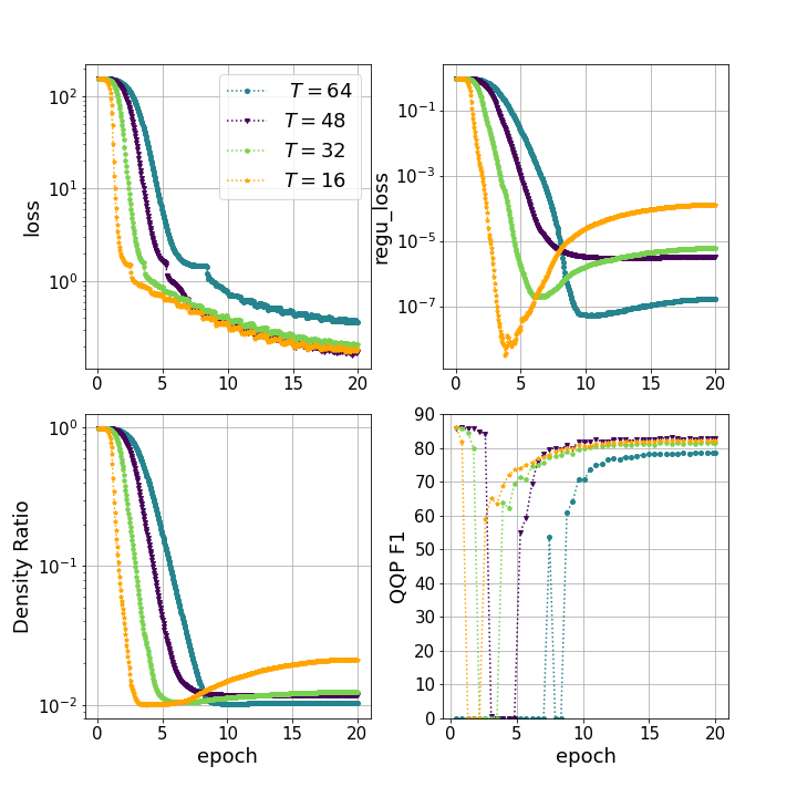
Figure 1: Effect of temperature $T$ for unstructured pruning on QQP. The density ratio is set to be 1%.

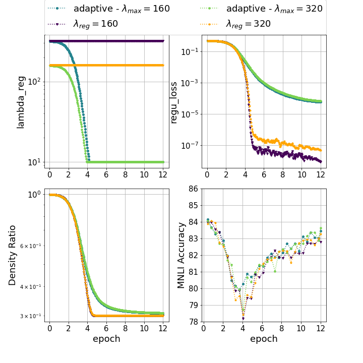
Figure 2: Effect of adaptive regularization $T$ for Hybrid pruning (H₃₂) on MNLI with a target dense ratio of $30\%$. Note that in the plot of density ratio with respect to epochs (left bottom), the purple (blue) and orange (green) curves are overlapped. Also in the right top bottom, blue and green curves are overlapped.

Temperature $T$

As $T$ defined in Eq. 3.2, it plays a critical role in determining the rate at which the threshold curve $k(\sigma_{i})$ falls. In addition, $T$ also directly links to the initialization of $\sigma_{i}$ which is set to be $5T$ for all $i$ such that $\text{Sigmoid}(\sigma_{i}/T)\approx 1$. This allows the model to have sufficient time to identify the layers which are insensitive for aggressive pruning and vice versa. To understand how $T$ influences the performances of the Bert model, we conduct an unstructured pruning on the QQP dataset by varying $T\in\{64,48,32,16\}$ and keeping all other hyperparameters to be the same. We plot the objective loss $\mathcal{L}_{\text{obj}}$ (loss), the regularization loss $\mathcal{L}_{\text{reg}}$ (regu_loss), the density ratio $R(\bm{\sigma})$, and F1 accuracy, with respect to the iterations in Figure 1.

Table 4: Unstructured pruning on SQuAD with epoch 10 using various values of regularization coefficient $\lambda_{reg}$ in Eq. 6. It shows that our LEAP is not too sensitive to the hyper-parameter choices $T$ and $\lambda_{reg}$.

Temperature $\lambda_{reg}=50$ $\lambda_{reg}=160$ $\lambda_{reg}=320$ acc/f1 density acc/f1 density acc/f1 density $T=16$ 76.58/84.94 10.66 76.49/85.01 10.27 76.33/84.85 10.2 $T=32$ 77.11/85.49 11.46 76.97/85.47 10.39 76.96/85.36 10.23

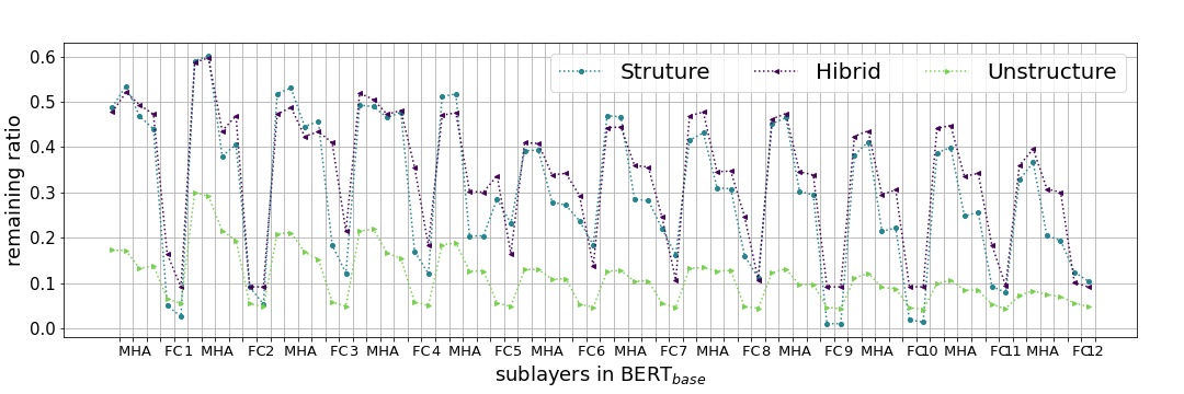
Figure 3: The density ratio $k(\sigma_{i})$ to all the weight matrices for structured, hybrid and unstructured pruning on SQuAD, of which the total density ratios are respectively 20% , 16%, and 8%.

Among the four curves in Figure 1, $T=48$ gives the best F1 accuracy while achieving $\sim$1% density, which clearly demonstrates the significance of $T$ for LEAP. Meanwhile, we see that the gaps between the performance for all $T$ except $64$ are close, thus it shows that LEAP is not sensitive to $T$. A possible explanation why $T=64$ gives the worse performance is that the density ratio of $T=64$ decays relatively slower compared to rest curves. As such, when it is close to the desired pruning regime, the learning rate is relatively small and so it cannot be able to recover the accuracy. On the other hand, it is interesting to note that using the temperature $T=16$ (orange curve), the density ratio increases after around five epochs and keeps increasing to the end, which results in a much better performance even though it experiences the most accuracy drop in the beginning. This in some scenes illustrates the “competition" between $\sigma_{i}$ in $\mathcal{L}_{\text{pure}}$ and $\sigma_{i}$ in $\mathcal{L}_{reg}$ mentioned in Section 3.2: the accuracy increases at epoch $5$ meaning that $\mathcal{L}_{\text{pure}}$ is decreasing effectively and the $\mathcal{L}_{reg}$ increases (compromises). Compared to those manual scheduling thresholds, this increasing phenomena of $\sigma_{i}$ also shows the advantage of learnable thresholds verifying that the model can figure out automatically when to prune and when not.

Robustness of hyper-parameter tuning $T$ and $\lambda_{reg}$

We see in the previous section that given the same $\lambda_{reg}$, various values of the temperature $T$ lead to similar results although tuning is necessary to achieve the best one. Here we study how robust the coefficient of $\lambda_{reg}$ in our proposed regularization $\mathcal{L}_{reg}$. We prune BERT${}_{\text{base}}$ on the SQuAD task with a target ratio $10\%$ with a combination of $\lambda_{reg}\in\{50,160,320\}$ and $T\in\{16,32\}$, for which the results is in Table 4.

For a given $T$, it indicates that the results are not highly sensitive to different $\lambda_{reg}$s as there is only about 0.1 variation for accuracy. It is worth noticing that a smaller $\lambda_{reg}$ (here $\lambda_{reg}=50$) can indeed affect achieving our target sparse ratio. However, the most off pruning ratio is 11.46%, which is reasonably close to the desired target of 10%.

For a given $\lambda_{reg}$, larger $T$ leads both the accuracy and the density ratio higher as expected. The reason is that the density ratio function, i.e., Sigmoid$(\sigma_{i}/T)$, becomes flatter for larger $T$, which leads to a higher density ratio by using the same value of $\sigma$ (Generally, $\sigma$ is negative to achieve $<50\%$ density ratio). And higher density ratio results in higher accuracy.

Overall, we can see that LEAP is robust to both $T$ and $\lambda_{reg}$.

The regularization coefficient $\lambda_{reg}$

To better understand the effect of adaptive $\lambda_{reg}$ (Eq. 7), we set $\lambda_{max}\in\{160,320\}$ and fix $\lambda_{min}=10$ (same as Section 5) to prune BERT${}_{\text{base}}$ on the MNLI task with a target ratio $30\%$. In addition, we also compare this adaptive coefficient with their constant counterparts $\lambda_{reg}\in\{160,320\}$. We plots the $\lambda_{reg}$ (lambda_reg), the regularization loss $\mathcal{L}_{\text{reg}}$ (regu_loss), the density ratio $R(\bm{\sigma})$, and accuracy, with respect to the iterations in Figure 2. First of all, we see that our adaptive coefficient $\lambda_{reg}$ decreases in a quadratic manner and reaching to the $\lambda_{min}=10$ after 4 epochs, which slows down the pruning activities after $4$ epochs. Also, note that the curves of different $\lambda_{max}$ are actually overlapped with each other, which also indicates that LEAP is not vulnerable to $\lambda_{reg}$. Meanwhile, as $\lambda_{reg}$ quickly reaches $\lambda_{min}$, the importance score $\mathcal{S}$ has more time to figure out the pruning parameters for the last small portion. As such, this slowness can in turn decrease the drop of accuracy and thus eventually recover a much better accuracy than that of the constant regularization.

The effect of learnable pruning for different weight matrices

As mentioned, the sensitivities of different weight matrices are different. Therefore, a high pruning ratio should be set for insensitive layers, and a low pruning ratio needs to be used for sensitive layers. To demonstrate LEAP can automatically achieve this, we plot the remaining parameters per layer for different pruning granularity on SQuAD in Figure 3. As can be seen, different layers receive different pruning ratios. Particularly, (i) as compared to MHA layers, FC layers are generally pruned more, which results in a lower density ratio. This might indicate that FC layers are less sensitive as compared to MHA layers; (ii) there is a clear trend that shallow layers (close to inputs) have higher density ratios as compared to deep layers (close to outputs). This finding is very intuitive. If the pruning ratio is too high for shallow layers, the information loss might be too high, and it is hard for the model to propagate the information to the output layer successfully. Therefore, the pruning ratio of shallow layers is smaller.

7 Conclusions

In this work, we present LEAP, a learnable pruning framework for transformer-based models. To alleviate the hyperparameter tuning effort, LEAP (i) introduces a novel regularization function to achieve desired pruning ratio with learnable pruning ratios for different weight matrices, and (ii) designs an adaptive regularization magnitude coefficient to control the regularization loss adaptively. By combining these two techniques, LEAP achieves on-par or even better performance for various pruning scenarios as compared to previous methods. Also, we demonstrate that LEAP less sensitive to the newly introduced hyperparameters and show the advance of the proposed adaptive regularization coefficient. Finally, we also show that there is clear pruning sensitivity associated with the depth and the component of the network.

Appendix A Training Details

For all three tasks, the temperature parameter $T$ for $k(\sigma_{i})$ is chosen between $\{16,32,48,64\}$ and $\lambda_{\max}$ varies between $\{40,80,160,320\}$ with $\lambda_{\min}=10$. For initialization of $\sigma_{i}$, we set it to be $5T$. We use a batch size 32, a sequence 128 for QQP/MNLI and 11000/12000 warmup steps (about 1 epoch) for learning rate. As for SQuAD, we use a batch size 16 and a sequence 384, and we use 5400 warmup steps (about 1 epoch). We use a learning rate of 3e-5 (1e-2) for the original weights (for pruning-rated parameters, i.e., $\mathcal{S}$ and $\bm{\sigma}$). We set all the training to be deterministic with the random seed of $17$. All the models are trained using FP32 with PyTorch on a single V100 GPU. Note that these configurations strictly follow the experimental setup in (Sanh et al., 2020; Lagunas et al., 2021); readers could check more details there. For the results in Table 1, the entire epoch using LEAP is 10, 6, and 10, respectively, for QQP, MNLI, and SQuAD. For the results of LEAP-1 and the results in Table 2, we simply double training epochs correspondingly (i.e., 20, 12, and 20).

Appendix B Results Details

Smaller tasks.

Note larger datasets (QQP/MNLI/SQuAD) to evaluate the performance of the pruning method is very common due to the evaluation robustness. However, to illustrate the generalization ability of LEAP, we also tested its performance on two smaller datasets STS-B and MPRC, using block pruning with size 32x32. The results are shown in Table 1. As can be seen, with around 20% density ratio, LEAP still achieves marginal accuracy degradation compared to baseline.

Table 5: Results for STS-B (baseline is 88.71) and MRPC (baseline is 87.01%) with different temperature $T$ and adaptive $\lambda_{max}$ for structure pruning (block size 32x32).

	Spearman correlation				Density ratio
STS-B	T=1	T=2	T=4		T=1	T=2	T=4
$\lambda_{max}=$80	85.68	85.86	85.96		20.0	20.1	22.5
$\lambda_{max}=$160	85.73	85.91	86.19		20.0	20.1	26.0
$\lambda_{max}=$320	85.72	86.01	86.46		20.0	20.3	28.5
	Accuracy				Density ratio
MRPC	T=1	T=2	T=4		T=1	T=2	T=4
$\lambda_{max}=$80	82.1	82.6	79.16		20.0	20.0	20.3
$\lambda_{max}=$160	81.37	82.35	79.65		20.0	20.0	21.3
$\lambda_{max}=$320	80.88	81.37	78.67		20.0	20.0	22.7

Hyper-parameter.

We emphasize again the results of soft mvp is a strong baseline, and our goal is not to purely beat soft mvp from accuracy perspective. However, their results require extensive hyperparameter tuning (see directory), while ours require to only tune $T$. To show the generalization of the best hyperparameter, we include the results for various $\lambda_{max}$ and $T$ on multiple tasks in Table 3. Note that when $T$ is fixed, different $\lambda_{max}$ gives similar results over various tasks.

Table 6: Results for QQP and MRPC with different temperature $T$ and adaptive $\lambda_{max}$ for structure pruning (block size 32x32).

	Accuracy				Density ratio
QQP	T=16	T=32	T=48		T=16	T=32	T=48
$\lambda_{max}$=160	90.68	90.87	90.7		20.07	20.07	20.1
$\lambda_{max}$=320	90.79	90.78	90.6		20.08	20.06	20.1
	Accuracy (MNLI/MNLI-MM)				Density ratio
MNLI	T=16	T=32	T=48		T=16	T=32	T=48
$\lambda_{max}$=40	80.41/81.06	80.79/81.12	80.87/81.22		21.07	21.52	22.25
$\lambda_{max}$=160	80.56/80.98	80.88/80.81	81.02/81.17		21.07	21.46	22.15

References

- Bai et al. (2020) Bai, H., Zhang, W., Hou, L., Shang, L., Jin, J., Jiang, X., Liu, Q., Lyu, M., and King, I. BinaryBERT: Pushing the limit of BERT quantization. arXiv preprint arXiv:2012.15701, 2020.
- Bengio et al. (2013) Bengio, Y., Léonard, N., and Courville, A. Estimating or propagating gradients through stochastic neurons for conditional computation. arXiv preprint arXiv:1308.3432, 2013.
- Bhandare et al. (2019) Bhandare, A., Sripathi, V., Karkada, D., Menon, V., Choi, S., Datta, K., and Saletore, V. Efficient 8-bit quantization of transformer neural machine language translation model. arXiv preprint arXiv:1906.00532, 2019.
- Brown et al. (2020) Brown, T. B., Mann, B., Ryder, N., Subbiah, M., Kaplan, J., Dhariwal, P., Neelakantan, A., Shyam, P., Sastry, G., Askell, A., et al. Language models are few-shot learners. arXiv preprint arXiv:2005.14165, 2020.
- Chen et al. (2020) Chen, T., Frankle, J., Chang, S., Liu, S., Zhang, Y., Wang, Z., and Carbin, M. The lottery ticket hypothesis for pre-trained BERT networks. arXiv preprint arXiv:2007.12223, 2020.
- Devlin et al. (2019) Devlin, J., Chang, M.-W., Lee, K., and Toutanova, K. BERT: Pre-training of deep bidirectional transformers for language understanding. In NAACL-HLT, 2019.
- Dong et al. (2017) Dong, X., Chen, S., and Pan, S. Learning to prune deep neural networks via layer-wise optimal brain surgeon. In Advances in Neural Information Processing Systems, pp. 4857–4867, 2017.
- Esser et al. (2019) Esser, S. K., McKinstry, J. L., Bablani, D., Appuswamy, R., and Modha, D. S. Learned step size quantization. arXiv preprint arXiv:1902.08153, 2019.
- Fan et al. (2019) Fan, A., Grave, E., and Joulin, A. Reducing transformer depth on demand with structured dropout. arXiv preprint arXiv:1909.11556, 2019.
- Fan et al. (2020) Fan, A., Stock, P., Graham, B., Grave, E., Gribonval, R., Jegou, H., and Joulin, A. Training with quantization noise for extreme fixed-point compression. arXiv preprint arXiv:2004.07320, 2020.
- Frankle & Carbin (2018) Frankle, J. and Carbin, M. The lottery ticket hypothesis: Finding sparse, trainable neural networks. arXiv preprint arXiv:1803.03635, 2018.
- Han et al. (2015) Han, S., Pool, J., Tran, J., and Dally, W. Learning both weights and connections for efficient neural network. In Advances in neural information processing systems, pp. 1135–1143, 2015.
- Han et al. (2016) Han, S., Mao, H., and Dally, W. J. Deep compression: Compressing deep neural networks with pruning, trained quantization and huffman coding. International Conference on Learning Representations, 2016.
- He et al. (2018) He, Y., Lin, J., Liu, Z., Wang, H., Li, L.-J., and Han, S. Amc: Automl for model compression and acceleration on mobile devices. In Proceedings of the European Conference on Computer Vision (ECCV), pp. 784–800, 2018.
- Hinton et al. (2014) Hinton, G., Vinyals, O., and Dean, J. Distilling the knowledge in a neural network. Workshop paper in NIPS, 2014.
- Huang & Wang (2018) Huang, Z. and Wang, N. Data-driven sparse structure selection for deep neural networks. In Proceedings of the European conference on computer vision (ECCV), pp. 304–320, 2018.
- Iandola et al. (2020) Iandola, F. N., Shaw, A. E., Krishna, R., and Keutzer, K. W. SqueezeBERT: What can computer vision teach NLP about efficient neural networks? arXiv preprint arXiv:2006.11316, 2020.
- Iyer et al. (2017) Iyer, S., Dandekar, N., and Csernai, K. First quora dataset release: Question pairs, 2017. URL https://data. quora. com/First-Quora-Dataset-Release-Question-Pairs, 2017.
- Jiao et al. (2019) Jiao, X., Yin, Y., Shang, L., Jiang, X., Chen, X., Li, L., Wang, F., and Liu, Q. TinyBERT: Distilling BERT for natural language understanding. arXiv preprint arXiv:1909.10351, 2019.
- Kitaev et al. (2020) Kitaev, N., Kaiser, Ł., and Levskaya, A. Reformer: The efficient transformer. arXiv preprint arXiv:2001.04451, 2020.
- Lagunas et al. (2021) Lagunas, F., Charlaix, E., Sanh, V., and Rush, A. M. Block pruning for faster transformers. In Proceedings of the 2021 Conference on Empirical Methods in Natural Language Processing, pp. 10619–10629, 2021.
- Lan et al. (2019) Lan, Z., Chen, M., Goodman, S., Gimpel, K., Sharma, P., and Soricut, R. ALBERT: A lite bert for self-supervised learning of language representations. In International Conference on Learning Representations, 2019.
- Lee et al. (2018) Lee, N., Ajanthan, T., and Torr, P. H. Snip: Single-shot network pruning based on connection sensitivity. arXiv preprint arXiv:1810.02340, 2018.
- Lin et al. (2018) Lin, S., Ji, R., Li, Y., Wu, Y., Huang, F., and Zhang, B. Accelerating convolutional networks via global & dynamic filter pruning. In IJCAI, pp. 2425–2432, 2018.
- Luo et al. (2017) Luo, J.-H., Wu, J., and Lin, W. Thinet: A filter level pruning method for deep neural network compression. In Proceedings of the IEEE international conference on computer vision, pp. 5058–5066, 2017.
- Michel et al. (2019) Michel, P., Levy, O., and Neubig, G. Are sixteen heads really better than one? arXiv preprint arXiv:1905.10650, 2019.
- Microsoft & Nvidia (2021) Microsoft and Nvidia. Using DeepSpeed and Megatron to Train Megatron-Turing NLG 530B, the World’s Largest and Most Powerful Generative Language Model. https://developer.nvidia.com/blog/using-deepspeed-and-megatron-to-train-megatron-turing-nlg-530b-the-worlds-largest-and-most-powerful-generative-language-model/, 2021.
- Narang et al. (2017) Narang, S., Undersander, E., and Diamos, G. Block-sparse recurrent neural networks. arXiv preprint arXiv:1711.02782, 2017.
- Park et al. (2020) Park, S., Lee, J., Mo, S., and Shin, J. Lookahead: a far-sighted alternative of magnitude-based pruning. arXiv preprint arXiv:2002.04809, 2020.
- Prasanna et al. (2020) Prasanna, S., Rogers, A., and Rumshisky, A. When BERT plays the lottery, all tickets are winning. arXiv preprint arXiv:2005.00561, 2020.
- Raffel et al. (2019) Raffel, C., Shazeer, N., Roberts, A., Lee, K., Narang, S., Matena, M., Zhou, Y., Li, W., and Liu, P. J. Exploring the limits of transfer learning with a unified text-to-text transformer. arXiv preprint arXiv:1910.10683, 2019.
- Rajpurkar et al. (2016) Rajpurkar, P., Zhang, J., Lopyrev, K., and Liang, P. Squad: 100,000+ questions for machine comprehension of text. arXiv preprint arXiv:1606.05250, 2016.
- Sajjad et al. (2020) Sajjad, H., Dalvi, F., Durrani, N., and Nakov, P. Poor man’s BERT: Smaller and faster transformer models. arXiv preprint arXiv:2004.03844, 2020.
- Sanh et al. (2019) Sanh, V., Debut, L., Chaumond, J., and Wolf, T. DistilBERT, a distilled version of bert: smaller, faster, cheaper and lighter. arXiv preprint arXiv:1910.01108, 2019.
- Sanh et al. (2020) Sanh, V., Wolf, T., and Rush, A. M. Movement pruning: Adaptive sparsity by fine-tuning. arXiv preprint arXiv:2005.07683, 2020.
- Shen et al. (2020) Shen, S., Dong, Z., Ye, J., Ma, L., Yao, Z., Gholami, A., Mahoney, M. W., and Keutzer, K. Q-BERT: Hessian based ultra low precision quantization of bert. In AAAI, pp. 8815–8821, 2020.
- Shen et al. (2021) Shen, S., Yao, Z., Kiela, D., Keutzer, K., and Mahoney, M. W. What’s hidden in a one-layer randomly weighted transformer? arXiv preprint arXiv:2109.03939, 2021.
- Shoeybi et al. (2019) Shoeybi, M., Patwary, M., Puri, R., LeGresley, P., Casper, J., and Catanzaro, B. Megatron-LM: Training multi-billion parameter language models using gpu model parallelism. arXiv preprint arXiv:1909.08053, 2019.
- Sun et al. (2019) Sun, S., Cheng, Y., Gan, Z., and Liu, J. Patient knowledge distillation for bert model compression. arXiv preprint arXiv:1908.09355, 2019.
- Sun et al. (2020) Sun, Z., Yu, H., Song, X., Liu, R., Yang, Y., and Zhou, D. MobileBERT: a compact task-agnostic BERT for resource-limited devices. arXiv preprint arXiv:2004.02984, 2020.
- Tang et al. (2019) Tang, R., Lu, Y., Liu, L., Mou, L., Vechtomova, O., and Lin, J. Distilling task-specific knowledge from BERT into simple neural networks. arXiv preprint arXiv:1903.12136, 2019.
- Vaswani et al. (2017) Vaswani, A., Shazeer, N., Parmar, N., Uszkoreit, J., Jones, L., Gomez, A. N., Kaiser, Ł., and Polosukhin, I. Attention is all you need. In Advances in neural information processing systems, pp. 5998–6008, 2017.
- Wang et al. (2020a) Wang, H., Zhang, Z., and Han, S. Spatten: Efficient sparse attention architecture with cascade token and head pruning. arXiv preprint arXiv:2012.09852, 2020a.
- Wang et al. (2020b) Wang, S., Li, B., Khabsa, M., Fang, H., and Ma, H. Linformer: Self-attention with linear complexity. arXiv preprint arXiv:2006.04768, 2020b.
- Wang et al. (2019) Wang, Z., Wohlwend, J., and Lei, T. Structured pruning of large language models. arXiv preprint arXiv:1910.04732, 2019.
- Williams et al. (2017) Williams, A., Nangia, N., and Bowman, S. R. A broad-coverage challenge corpus for sentence understanding through inference. arXiv preprint arXiv:1704.05426, 2017.
- Xiao et al. (2019) Xiao, X., Wang, Z., and Rajasekaran, S. Autoprune: Automatic network pruning by regularizing auxiliary parameters. In Advances in Neural Information Processing Systems, pp. 13681–13691, 2019.
- Yu et al. (2019) Yu, H., Edunov, S., Tian, Y., and Morcos, A. S. Playing the lottery with rewards and multiple languages: lottery tickets in rl and nlp. arXiv preprint arXiv:1906.02768, 2019.
- Yu et al. (2018) Yu, R., Li, A., Chen, C.-F., Lai, J.-H., Morariu, V. I., Han, X., Gao, M., Lin, C.-Y., and Davis, L. S. Nisp: Pruning networks using neuron importance score propagation. In Proceedings of the IEEE Conference on Computer Vision and Pattern Recognition, pp. 9194–9203, 2018.
- Yu et al. (2021) Yu, S., Yao, Z., Gholami, A., Dong, Z., Mahoney, M. W., and Keutzer, K. Hessian-aware pruning and optimal neural implant. arXiv preprint arXiv:2101.08940, 2021.
- Zadeh et al. (2020) Zadeh, A. H., Edo, I., Awad, O. M., and Moshovos, A. Gobo: Quantizing attention-based nlp models for low latency and energy efficient inference. In 2020 53rd Annual IEEE/ACM International Symposium on Microarchitecture (MICRO), pp. 811–824. IEEE, 2020.
- Zafrir et al. (2019) Zafrir, O., Boudoukh, G., Izsak, P., and Wasserblat, M. Q8BERT: Quantized 8bit bert. arXiv preprint arXiv:1910.06188, 2019.
- Zhang et al. (2020) Zhang, W., Hou, L., Yin, Y., Shang, L., Chen, X., Jiang, X., and Liu, Q. Ternarybert: Distillation-aware ultra-low bit bert. arXiv preprint arXiv:2009.12812, 2020.
- Zhao et al. (2019) Zhao, C., Ni, B., Zhang, J., Zhao, Q., Zhang, W., and Tian, Q. Variational convolutional neural network pruning. In Proceedings of the IEEE Conference on Computer Vision and Pattern Recognition, pp. 2780–2789, 2019.
- Zhao et al. (2020) Zhao, M., Lin, T., Mi, F., Jaggi, M., and Schütze, H. Masking as an efficient alternative to finetuning for pretrained language models. arXiv preprint arXiv:2004.12406, 2020.
- Zhu & Gupta (2017) Zhu, M. and Gupta, S. To prune, or not to prune: exploring the efficacy of pruning for model compression. arXiv preprint arXiv:1710.01878, 2017.