A learning-based projection method for model order reduction of transport problems

Abstract

The Kolmogorov $n$-width of the solution manifolds of transport-dominated problems can decay slowly. As a result, it can be challenging to design efficient and accurate reduced order models (ROMs) for such problems. To address this issue, we propose a new learning-based projection method to construct nonlinear adaptive ROMs for transport problems. The construction follows the offline-online decomposition. In the offline stage, we train a neural network to construct adaptive reduced basis dependent on time and model parameters. In the online stage, we project the solution to the learned reduced manifold. Inheriting the merits from both deep learning and the projection method, the proposed method is more efficient than the conventional linear projection-based methods, and may reduce the generalization error of a solely learning-based ROM. Unlike some learning-based projection methods, the proposed method does not need to take derivatives of the neural network in the online stage.

Keywords— reduced order model; transport problems; deep learning; neural network; projection method; adaptive

1 Introduction

The transport phenomena arise in many important areas of applications, such as fluid dynamics, plasma physics and electromagnetics. Efficient and accurate reduced order models (ROMs) of transport-dominated problems are highly desired. However, as pointed out by [3, 42, 21, 13], the Kolmogorov $n$-width [44] of the solution manifold for a transport problem may decay slowly. If one applies conventional ROM strategies such as proper orthogonal decomposition (POD) methods [4, 22] or reduced basis methods (RBM) [24] straightforwardly, linear subspaces of rather high dimensions will be needed to obtain accurate reduced order approximations. The design of a model with genuine reduced order for transport problems is hence challenging.

Overcoming this difficulty has been an active research topic in the ROM community, where two general ideas have been extensively considered: 1) to introduce online adaptivity to the reduced solution space, and 2) to identify and conduct inherent nonlinear transformations which enable the construction of efficient ROMs. Examples following the former include [10] and [43], where [10] adaptively enriches the reduced basis in the online stage through splitting while [43] applies online adaptive sampling and basis reconstruction based on a local low-rank structure. Examples following the latter direction include the shift POD method [45], which utilizes a shift operator determined by the underlying wave speed. Such information is also utilized under a Lagrangian framework in designing the Lagrangian POD [37], the Lagrangian DMD [31] and its recent extension to the case with shocks [32]. Besides, nonlinear transformations can also be obtained by the method of freezing [50, 41, 5], the transformed snapshot interpolation [60, 61, 62], the approximated Lax pairs [18, 19], template fitting [27, 51], the transport reversal method [46], shock fitting [55], the registration method [54, 57, 16], and the greedy Wasserstein barycenter algorithm [15].

Our proposed method is inspired by the series of work [8, 7, 9, 40], and is also closely related to [47, 39, 57, 38, 54, 16]. The key underlying idea of [8, 7, 9, 40] is that, for a transport-dominated problem, there exists some suitable nonlinear transformation $T_{t,\mu}$, under which the transformed solution manifold displays a much faster decay in its Kolmogorov $n$-width and hence can be accurately approximated by a low-dimensional reduced space. Once the transformation is obtained by some means, a reduced order approximation is constructed in the form of

$$u_{r}(x,t;\mu)=\sum_{i=1}^{r}\alpha_{i}(t,\mu)\psi_{i}(T_{t,\mu}(x;t,\mu))=\sum_{i=1}^{r}\alpha_{i}(t,\mu)\phi_{i}(x;t,\mu).$$ (1.1)

Here, $x$ is the physical location, $t$ is time, $\mu$ is a scalar or vector-valued model parameter. Each $\psi_{i}$ is a reduced basis function in the transformed space and $\phi_{i}(x;t,\mu)=\psi_{i}(T_{t,\mu}(x;t,\mu))$ is the respective reduced basis function in the original solution manifold. The distinct feature of the adaptive reduced basis $\{\phi_{i}(x;t,\mu)\}_{i=1}^{r}$ is that each member depends on time $t$ and the model parameter $\mu$, in addition to $x$. The nonlinear transformation $T_{t,\mu}$ can be realized as coordinate transformations defined case by case, such as for the 2D Euler equations in [8], the 1D Burgers equation in [9] and the Navier-Stokes equations in [40]. The manifold approximations via transported subspaces (MATS) [47], on the other hand, construct the nonlinear transformation with an optimal transport tool called displacement interpolation [35, 58], while the transported snapshot method [39] applies a polynomial approximation in such constructions. The Lagrangian registration based method [54, 16], the ALE registration method [57] and the ALE autoencoder [38] construct $T_{t,\mu}$ by solving nonlinear optimization problems.

In this paper, we propose a new framework to design nonlinear reduced order models for transport problems by working with an adaptively constructed reduced basis $\{\phi_{i}(x;t,\mu)\}_{i=1}^{r}$. The framework can be decomposed into an offline stage and an online stage. In the offline stage, instead of predetermining or seeking the transformation $T_{t,\mu}$, the adaptive basis will be learned directly from data with neural networks, since the ultimate goal is to obtain the reduced order space. More specifically, $\{\alpha_{i}(t,\mu)\}_{i=1}^{r}$ and $\{\phi_{i}(x;t,\mu)\}_{i=1}^{r}$ in (1.1) will be parameterized separately as feed-forward neural networks taking $t,\mu$ or $x,t,\mu$ as inputs, and these neural networks will be trained with snapshot solutions (e.g. high-fidelity numerical solutions). In the online stage, instead of making predictions entirely with the trained neural networks as in a pure learning-based method, we only take the learned basis $\{\phi_{i}(x;t,\mu)\}_{i=1}^{r}$ to construct a subspace that is local to $t$ and $\mu$, and apply the standard projection method to find the reduced order approximation. The performance of the proposed method is demonstrated numerically through a series of linear and nonlinear scalar hyperbolic conservation laws in 1D and 2D as well as the 1D compressible Euler system. The methodology developed here can also be applied to obtain reduced order approximations for other transport problems. Unlike the aforementioned methods that explicitly identify $T_{t,\mu}$ to build ROMs, our proposed method only learns the basis and the corresponding reduced order space, with the information of the transformation $T_{t,\mu}$ implicitly encoded in the learned space. Identifying $T_{t,\mu}$ can sometimes be helpful, but the explicit form of it is not always necessary.

The proposed learning-based projection method is a combination of the deep learning method and the standard projection method. Compared with a conventional projection method (e.g. POD), or a solely learning-based method, the proposed method has several advantages in constructing ROMs. Our numerical experiments show that the proposed method is more accurate than the standard POD method for long time predictions with a similar order reduction. The reason behind is that the inherent nonlinear information of the underlying transport problems can be implicitly embedded in the adaptive basis through training while a conventional linear projection method may suffer from the slow decay of the Kolmogorov $n$-width. Particularly, we observe that the adaptive basis obtained in fact travels at the underlying wave speed for a simple 1D linear advection equation. Another advantage over the conventional projection method is that the neural network takes $x$ as an input in a mesh-free manner, hence it is simple and flexible to work with different meshes in the online and offline stages, or even learn from experimental mesh-free data. Comparing with a pure learning-based approach, our method can reduce the generalization error due to overfitting with an online projection procedure utilizing the underlying PDE information.

We also want to point out that we are not the first to combine projection methods with the deep learning techniques to build ROMs for transport problems. In [28, 29, 26], auto-encoders were used to learn a low-dimensional nonlinear approximation of the solution manifold offline, and a reduced-order solution can then be obtained through an online projection . The main differences between our method and aforementioned methods are as follows. First, [28, 29, 26] are based on a different reduced-order representation. Second, in the online computations, different from our method, these methods need to take the derivative of the decoder neural network, and this could be computationally expensive. To improve their online efficiency, [26] uses a decoder with a shallow architecture and applies hyper-reduction techniques. Third, compared with these methods, our method does not require using the same spatial meshes at online and offline stages, and is thus advantageous for moving mesh methods or $h$-adaptive simulations with locally refined meshes. Similar ideas as in [28, 29, 26] are also utilized to develop a learning based ROM [17] under a pure data-driven framework. There, a reduced order nonlinear trial manifold is constructed by the decoder part of an auto-encoder trained offline. Instead of using a projection-based method online, [17] evolves the coordinate in the low-dimensional latent space through an extra neural network which is trained offline to learn the reduced dynamics. This data-driven online phase is more efficient than the projection based online algorithm in [28, 29, 26] and our method, but may suffer from larger generalization errors. Another interesting work that uses deep learning to construct ROMs for transport problems is [48], which utilizes ideas similar to the MATS [47] to lighten the architectures of neural networks.

The main difference between our method and the optimal transport based method [47], optimization based registration/autoencoder [57, 54, 38, 16] and the transported snapshot method [39] is that we find the adaptive reduced order space without explicitly finding the transformation, while they explicitly find the transformation. We use a neural network ansatz for the adaptive reduced basis, while these methods use different ansatz. Our method can be seen as an alternative to these methods. We would also like to make more comments about the optimal transport based methods [15, 47]. Compared with deep learning based methods, these optimal transport based methods are more interpretable, and theoretical understandings have been established. However, more developments are still needed for more complicated transport problems. The greedy Wasserstein barycenter method [15] and its recent generalization to the nonconservative flows in porous media [2] are limited to 1D for now, as they use an exponential map only valid in 1D to efficiently compute the Wasserstein distance. The MATS method [47] transports reduced subspaces along characteristics and can not directly handle the case when characteristics intersect (e.g. problems with shocks). As demonstrated in our numerical examples, our proposed method can handle 2D problems and problems with shocks. We also want to mention that [48] generalizes [47] with deep learning techniques and could handle problems with shocks, but its connection with optimal transport becomes less clear.

The paper is organized as follows. In Section 2, we briefly review the basic idea of projection-based ROM methods and explain why designing an efficient ROM of transport problems could be challenging. Then, in Section 3, we present the offline and online algorithms of the proposed learning-based projection method as well as the neural network architecture. In Section 4, the performance of the proposed method is demonstrated through a series of numerical experiments. In Section 5, we draw our conclusions and discuss some potential future research directions.

2 Background

We consider a parametric time-dependent transport problem:

$${\color[rgb]{0,0,0}\textrm{residual}(u;\mu)=0,\;\mu\in X_{\mathcal{P}},}$$ (2.2)

where $\mu$ is a scalar or vector-valued model parameter and $\textrm{residual}(\cdot;\mu)$ represents a time-dependent parametric hyperbolic partial differential operator. The solution $u(x,t;\mu)$ depends on the location $x\in\Omega$, the time $t$ and the parameter $\mu$. To design a reduced order model, we assume a full order model is available, which is a high-fidelity numerical scheme solving (2.2) and can be written as

$${\color[rgb]{0,0,0}\textrm{residual}}_{h}(u_{h};\mu)=0$$ (2.3)

in its strong form. We view the solution $u_{h}(x,t;\mu)$ as the ground truth, and denote the solution manifold as $\{u_{h}(\cdot,t;\mu):0\leq t\leq T_{\textrm{max}},\mu\in X_{\mathcal{P}}\}$.

A conventional projection-based ROM seeks a solution in the form of

$$u_{r}(x,t;\mu)=\sum_{i=1}^{r}\alpha_{i}(t,\mu)\varphi_{i}(x).$$ (2.4)

Here, $r$ is the order of the reduced order model, $\{\varphi_{i}(x)\}_{i=1}^{r}$ is a reduced basis, with the expansion coefficients ${\boldsymbol{\alpha}}(t,\mu)=(\alpha_{1}(t,\mu),\dots,\alpha_{r}(t,\mu))^{T}$. The reduced basis depends on $x$, and is typically obtained through the offline training. The coefficients are then determined online through projection methods. Such procedure provides efficient and accurate reduced order models for problems whose solution manifolds have fast-decaying Kolmogorov $n$-width [36, 6].

However, it is well-known that the Kolmogorov $n$-width for transport-dominated problems may decay slowly [42, 3, 21, 13]. On the other hand, the evidence in [8] indicates that under some coordinate transformations, the transformed solution manifolds of transport-like problems can have much faster decay in their Kolmogorov $n$-width. This can be illustrated by the following simple example. Consider the 1D advection equation

$$u_{t}+u_{x}=0,\quad x\in[0,2],$$ (2.5)

with zero boundary conditions and the following initial condition

$$u(x,0)=u_{0}(x)=\begin{cases}1,\quad 0.25\leq x\leq 0.5,\\ 0,\quad\text{otherwise.}\end{cases}$$ (2.6)

The exact solution is $u(x,t)=u_{0}(x-t)$ (over the time period $[0,1]$ of our consideration). We introduce a uniform space-time mesh with $\Delta x=\Delta t=0.01$ and $x_{i}=i\Delta x$, $t_{j}=j\Delta t$, and use the exact solution sampled from this mesh over $t\in[0,1]$ to define the solution manifold, whose Kolmogorov n-width with respect to the $l_{2}$ norm is measured as the $n$-th singular value of the snapshot matrix $S=(s_{ij})$, with $s_{ij}=u(x_{i},t_{j})=u_{0}((i-j)\Delta x)$. Meanwhile, we can follow [8] and apply a $t$-dependent transformation $T(x;t)=x-t$, and obtain a transformed snapshot matrix $\tilde{S}=\{\tilde{s}_{ij}\}$ with

$$\tilde{s}_{ij}=u(T^{-1}(x_{i};t_{j}),t_{j})=u(x_{i}+t_{j},t_{j})=u_{0}(x_{i}).$$

In Figure 2.1, the singular values of the original and transformed snapshot matrices are presented. We observe that the singular values of the original snapshot matrix decay fairly slowly as expected, while those of the transformed snapshot matrix decay very fast. As a result, standard ROMs such as POD will require a fairly large reduced space for accurate approximation, yet with the help of the $t$-dependent transformation $T(x;t)$, the dimension of the reduced space can be dramatically reduced.

Figure 2.1: Singular values of the original and transformed snapshot matrices.

The approximation power of the standard reduced order spaces (e.g. the POD space) is limited as they are linearly expanded with basis functions that are static with respect to $t$ and $\mu$, see (2.4). As shown above, one way to conquer this limitation is to use a reduced order space with an adaptive time-and-parameter-dependent (i.e. ($t,\mu$)-dependent) basis $\{\phi_{i}(x;t,\mu)\}_{i=1}^{r}$, with the reduced order approximation given as:

$$u_{r}(x,t;\mu)=\sum_{i=1}^{r}\alpha_{i}(t,\mu)\phi_{i}(x;t,\mu).$$ (2.7)

In the series of paper [8, 9, 40], the basis used takes the form $\phi_{i}(x;t,\mu)=\psi_{i}(T_{t,\mu}(x))$, where $T_{t,\mu}$ is a suitable coordinate transformation defined problem by problem. Similar ideas have also been considered in [47, 39, 57, 54, 38, 16]. In [47], $T_{t,\mu}$ is constructed with the displacement interpolation [35, 58] while the polynomial approximation is used in [39]. The Lagrangian and arbitrary Lagrangian Eulerian (ALE) registration method [57, 54, 16] and the ALE autoencoder [38] find $T_{t,\mu}$ by solving optimization problems.

Following [8, 9, 40], we propose a learning-based projection method. To avoid designing suitable coordinate transformations $T_{t,\mu}$ a priori for each problem, we parameterize the basis functions $\{\phi_{i}(x;t,\mu)\}_{i=1}^{r}$ as a neural network ${\mathcal{N}\mathcal{N}}^{\phi}(x,t,\mu;\theta^{\phi})$ and determine the trainable parameters of the neural network $\theta^{\phi}$ in the offline learning stage. In the online stage, we further utilize a projection method to predict solutions either at a future time or corresponding to a new value of the model parameter $\mu$. The ROM algorithms will be detailed in Section 3.

3 Reduced order model algorithms

One natural extension to [8, 9, 40] is utilizing neural networks to learn a coordinate transformation $T_{t,\mu}$. However, it is nontrivial to measure how a coordinate transformation reduces the Kolmogorov $n$-width of the transformed solution manifold for a general problem with neural networks, not to mention to systematically find a good one. Instead, we directly learn the $(t,\mu)$-dependent adaptive basis, hence the adaptive reduced order space, using neural networks, while the transformation $T_{t,\mu}$ is implicitly encoded.

We follow the standard offline-online decomposition of the projection-based ROM method. In Section 3.1, we present the offline stage algorithm which obtains the adaptive basis by training two neural networks with snapshot solutions. In the online stage, with the learned $(t,\mu)$-dependent basis available, we apply a projection-based method to construct a reduced representation of the solution, and this will be detailed in Section 3.2. A discussion over the architecture of the neural network is then presented in Section 3.3.

3.1 Offline stage

In the offline training stage, the snapshot solutions are high-fidelity numerical solutions from a full order model. For the time-dependent transport problems considered in this work, we assume the full order model is given by a one-step scheme

$${\color[rgb]{0,0,0}\textrm{residual}_{h}(u_{h}^{n+1},u_{h}^{n};\mu)=0}$$ (3.8)

in its strong form, and it can be constructed through a finite difference/volume/element method, or a discontinuous Galerkin method. Here $u_{h}^{n}=u_{h}(x,t_{n};\mu)$ denotes the numerical solution at time $t_{n}$. The snapshot solutions can also be obtained from measurements or practical experiments.

Suppose we have the snapshot solutions, $u_{h}(x_{i},t_{j};\mu_{k})$, with

$$\{x_{i}\}_{i=0}^{N_{x}}\subset\Omega,\quad\{t_{j}\}_{j=1}^{N_{t}}\subset[0,T_{\textrm{train}}],\quad\{\mu_{k}\}_{k=1}^{N_{\mu}}\subset\mathcal{P}_{\textrm{train}}\subset X_{\mathcal{P}}.$$

Note that the spatial degrees of freedom of $u_{h}$ used here are nodal values. Our proposed framework can be adapted to ROMs with other types of spatial degrees of freedom, such as moments. Though the snapshot solutions are taken from $[0,T_{\textrm{train}}$], the proposed method may be applied to predict solutions at a future time $t>T_{\textrm{train}}$.

To obtain the $(t,\mu)$-dependent basis, we define the following $r$-th order neural network approximation:

$$u_{\mathcal{N}\mathcal{N}}(x,t;\mu,\boldsymbol{\theta}) =\sum_{i=1}^{r}{\alpha}^{\mathcal{N}\mathcal{N}}_{i}(t,\mu;{\color[rgb]{0,0,0}\theta^{\alpha}})\ {\phi}^{\mathcal{N}\mathcal{N}}_{i}(x,t,\mu;{\color[rgb]{0,0,0}\theta^{\phi}})$$

$$=\boldsymbol{{\alpha}^{\mathcal{N}\mathcal{N}}}(t,\mu;\theta^{\alpha})\cdot\boldsymbol{{\phi}^{\mathcal{N}\mathcal{N}}}(x,t,\mu;\theta^{\phi}).$$ (3.9)

Here, ${\color[rgb]{0,0,0}r}\ll N_{x}$ is the order of the ROM. $\boldsymbol{\theta}=(\theta^{\alpha},\theta^{\phi})$ are trainable parameters of the neural network. The $r$-dimensional vectors $\boldsymbol{{\alpha}^{\mathcal{N}\mathcal{N}}}=({\alpha}^{\mathcal{N}\mathcal{N}}_{1},\cdots,{\alpha}^{\mathcal{N}\mathcal{N}}_{r})^{T}$ and $\boldsymbol{{\phi}^{\mathcal{N}\mathcal{N}}}=({\phi}^{\mathcal{N}\mathcal{N}}_{1},\cdots,{\phi}^{\mathcal{N}\mathcal{N}}_{r})^{T}$ are the outputs of the neural networks ${\mathcal{N}\mathcal{N}}^{\alpha}(t,\mu;\theta^{\alpha})$ and ${\mathcal{N}\mathcal{N}}^{\phi}(x,t,\mu;\theta^{\phi})$, where ${\mathcal{N}\mathcal{N}}^{\alpha}(t,\mu;\theta^{\alpha})$ and ${\mathcal{N}\mathcal{N}}^{\phi}(x,t,\mu;\theta^{\phi})$ parameterize the expansion coefficients and the $(t,\mu)$-dependent basis, respectively. The neural network is trained by minimizing the mean-square loss function:

$${\color[rgb]{0,0,0}\boldsymbol{\theta^{*}}=(\theta^{\alpha,*},\theta^{\phi,*})=\arg\min_{\boldsymbol{\theta}}\frac{1}{(N_{x}+1)N_{t}N_{\mu}}\sum_{i=0}^{N_{x}}\sum_{j=1}^{N_{t}}\sum_{k=1}^{N_{\mu}}\big{(}u_{\mathcal{N}\mathcal{N}}(x_{i},t_{j};\mu_{k},\boldsymbol{\theta})-u_{h}(x_{i},t_{j};\mu_{k})\big{)}^{2}.}$$ (3.10)

The solution to the optimization problem in (3.10) is not unique in the sense that one can reorder and rescale basis functions. Keep in mind that what we truly want is not the basis itself but the associated adaptive reduced order space. In practice, the ordering and the scaling of the learned basis will be influenced by the random initialization of the neural networks. Also, due to the non-convex nature of the underlying minimization problem, the optimizer may converge to a low dimensional manifold corresponding to a local minimum. But at least for numerical tests being considered, these issues do not seem to pose any problem in the present work, either to the training of the neural networks or to the overall performance of the proposed algorithm. Nevertheless, it will be left to our future exploration to learn more structured basis functions such as an orthonormal basis.

Essentially, the neural network $u_{\mathcal{N}\mathcal{N}}(\cdot;\cdot,\mathbf{\theta^{*}})$ provides a reduced order model to approximate the true solution. However, due to the potential risk of over-fitting, the purely learning-based reduced approximation $u_{\mathcal{N}\mathcal{N}}$ is not always accurate and robust in generalization. We propose to only pass the learned adaptive basis $\{{\phi}^{\mathcal{N}\mathcal{N}}_{i}\}_{i=1}^{r}$ onward to the online stage.

It is worth noticing that ${\mathcal{N}\mathcal{N}}^{\phi}$ takes $x$ as one of its inputs in a mesh free manner, and therefore it is simple and flexible to work with solution snapshots obtained on different meshes tailored for different values of the model parameter, or even solution snapshots based on experimental data. However, a conventional projection-based method may need extra steps such as interpolations [20] or full order offline re-computations [64, 65] in order to work with snapshots subject to different meshes.

Remark 3.1.

For now, the reduced order $r$ is pre-selected. One way to adaptively determining $r$ is to apply a block-by-block training strategy similar to [14]. More specifically, start with a pre-selected small $r_{0}$ and train the neural network $u_{\mathcal{N}\mathcal{N}_{0}}=\sum_{i=1}^{r_{0}}{\alpha}^{\mathcal{N}\mathcal{N}}_{i}(t,\mu;\theta^{\alpha}){\phi}^{\mathcal{N}\mathcal{N}}_{i}(x,t,\mu;\theta^{\phi})$. If the prediction error of a validation set is too large with the pre-selected $r_{0}$, one can train a second neural network $u_{\mathcal{N}\mathcal{N}_{1}}=\sum_{i=r_{0}+1}^{r_{0}+\Delta r}{\alpha}^{\mathcal{N}\mathcal{N}}_{i}(t,\mu;\theta^{\alpha}){\phi}^{\mathcal{N}\mathcal{N}}_{i}(x,t,\mu;\theta^{\phi})$ by minimizing the mismatch between $u_{\mathcal{N}\mathcal{N}_{0}}+u_{\mathcal{N}\mathcal{N}_{1}}$ and the full order solution $u_{h}$. Repeat this procedure until the prediction error of the validation set is small enough or reach the maximum number of basis functions allowed.

Remark 3.2.

In practice, it is important to have an effective sampling strategy when the dimension of the problem or the parameter $\mu$ is high. In order to reduce the computational cost of sampling, one may apply an adaptive sampling strategy based on the greedy algorithm [34, 24] or the “data exploration” in [23]. Effective sampling strategy is not the focus of this paper, and for now, we do not apply these strategies and leave them for future investigations. Similarly, the terminal training time $T_{\textrm{train}}$ can also be adaptively determined, e.g. based on the validation error or an error estimator.

3.2 Online stage

In the online stage, we take the learned adaptive basis $\{{\phi}^{\mathcal{N}\mathcal{N}}_{i}\}_{i=1}^{r}$ and seek a reduced-order numerical solution in their span following a projection approach. For simplicity, we denote $\phi_{i}^{n+1}(x;\mu)=\phi_{i}^{\mathcal{N}\mathcal{N}}(x,t_{n+1},\mu;\theta^{\phi,*})$, $i=1,\cdots,r$. The reduced order space at $t_{n+1}$ associated with $\mu$ is then given as

$$V^{n+1}_{r}(\mu):=\text{span}\{\phi_{i}^{n+1}(\cdot;\mu)\}_{i=1}^{r}.$$

We also introduce $\boldsymbol{\Phi}_{\mu}^{n+1}\in\mathbb{R}^{(N_{x}+1)\times r}$, with its $(i,j)$-th entry being

$$\boldsymbol{\Phi}_{\mu}^{n+1}(i,j)=\phi_{j}^{n+1}(x_{i};\mu),\;\;i=0,\cdots,N_{x},\;\;j=1,\cdots,r.$$ (3.11)

Suppose the full order model (3.8) has the following matrix-vector form:

$$\boldsymbol{F}_{\mu}({\bf u}_{\mu}^{n+1})={\bf{b}}_{\mu}^{n},$$ (3.12)

where ${\bf{u}}_{\mu}^{n+1}\in\mathbb{R}^{N_{x}+1}$ is the vector of nodal values (i.e. the spatial degrees of freedom) of the numerical solution $u_{h}(x,t_{n+1};\mu)$ at $\{x_{j}\}_{j=0}^{N_{x}}$ and time $t_{n+1}$. ${\bf{b}}_{\mu}^{n}\in\mathbb{R}^{N_{x}+1}$ is a known vector determined by ${\bf{u}}_{\mu}^{n}$, and the operator $\boldsymbol{F}_{\mu}:\mathbb{R}^{N_{x}+1}\mapsto\mathbb{R}^{N_{x}+1}$ is derived from the full order model (3.8). We look for the reduced order approximation of the solution $u_{r,h}^{n+1}\in V^{n+1}_{r}(\mu)$, whose nodal values at $\{x_{j}\}_{j=0}^{N_{x}}$ (i.e. spatial degrees of freedom) are $\boldsymbol{\Phi}_{\mu}^{n+1}\boldsymbol{\alpha}^{n+1}$, with some $\boldsymbol{\alpha}^{n+1}=(\alpha_{1}^{n+1},\cdots,\alpha_{r}^{n+1})^{T}\in\mathbb{R}^{r}$. Following a projection method, we require

$$(\boldsymbol{\Phi}^{n+1}_{\mu})^{T}\boldsymbol{F}_{\mu}(\boldsymbol{\Phi}^{n+1}_{\mu}\boldsymbol{\alpha}^{n+1})=(\boldsymbol{\Phi}^{n+1}_{\mu})^{T}{\bf{b}}^{n}_{\mu}.$$ (3.13)

Once ${\boldsymbol{\alpha}}^{n+1}$ is calculated, we reach a reduced-order approximation of the solution at $t_{n+1}$: $u_{r,h}^{n+1}=\sum_{i=1}^{r}\alpha_{i}^{n+1}\phi_{i}^{n+1}$. The online algorithm is summarized in Algorithm 1.

1:Input: given the parameter $\mu$; assume the reduced order numerical solution $u_{r,h}^{n}$ at time $t_{n}$ is known, and it defines ${\bf{b}}_{\mu}^{n}$ in (3.12) based on the full order model (3.8).

2:Evaluate the $(t,\mu)$-dependent basis with the neural network ${\mathcal{N}\mathcal{N}}^{\phi}$ trained offline:

$${\color[rgb]{0,0,0}\phi_{i}^{n+1}}(x;\mu):={\phi}^{\mathcal{N}\mathcal{N}}_{i}(x,t_{n+1},\mu;\theta^{\phi,*}),\quad i=1,\cdots,r.$$ (3.14)

And form the matrix $\boldsymbol{\Phi}_{\mu}^{n+1}\in\mathbb{R}^{{(N_{x}+1)}\times r}$ as in (3.11).

3:Obtain $u_{r,h}^{n+1}$ through the projection: compute $\boldsymbol{\alpha}^{n+1}$ by

$$(\boldsymbol{\Phi}^{n+1}_{\mu})^{T}\boldsymbol{F}_{\mu}(\boldsymbol{\Phi}^{n+1}_{\mu}\boldsymbol{\alpha}^{n+1})=(\boldsymbol{\Phi}^{n+1}_{\mu})^{T}{\bf{b}}_{\mu}^{n}.$$ (3.15)

4:Output: the reduced order numerical solution at $t_{n+1}$ for the parameter $\mu$ is

$$u_{r,h}^{n+1}=\sum_{i=1}^{r}\alpha_{i}^{n+1}\phi_{i}^{n+1}.$$

Algorithm 1 Online projection for one time step update

Compared with a standard projection-based method such as the POD method, in the online stage, we have the extra step to evaluate the $(t,\mu)$-dependent basis with a trained neural network with known parameters $\theta^{\phi,*}$ at each time step $t_{n+1}$. In our numerical tests, we find that, even with this additional cost, our method still leads to computational savings compared with a full order model when the underlying mesh is well refined.

As mentioned before, the neural network ${\mathcal{N}\mathcal{N}}^{\phi}$ takes $x$ as one of its inputs in a mesh free manner. Although it is not deeply investigated in this work, the proposed method has the capability to be integrated with $h$-adaptive numerical schemes for time dependent problems in the online stage. In Section 4.3, the proposed method is combined with a moving mesh method to show its capability.

We also want to compare our proposed method with the learning-based projection methods in [28, 29, 26]. In the offline stage, taking the full order solution as the input, these methods find a low-dimensional nonlinear manifold to represent the full order solution manifold by training an auto-encoder. In the online stage, these methods seek a reduced order approximation in the form

$$u\approx u_{\textrm{ref}}+g(\hat{u}_{r}).$$ (3.16)

Here, $u_{\textrm{ref}}$ is a predetermined reference frame, $g$ is the decoder part of the neural-network trained offline, which is a mapping from a low-dimensional latent space to the high-dimensional solution manifold, and ${\color[rgb]{0,0,0}\hat{u}_{r}}$ can be seen as the coordinates in the low-dimensional latent space. In the online stage, these methods solve a minimal residual problem

$$\hat{u}_{r}^{n+1}=\arg\min||{\color[rgb]{0,0,0}\textrm{residual}}_{h}(g(\hat{u}_{r}^{n+1}),u_{h}^{n};\mu)||_{2}.$$ (3.17)

To obtain $\hat{u}^{n+1}_{r}$, [28, 29] need to take the derivatives or even the second order derivatives of the neural-network $g$ online, which can be computationally expensive. To improve the online efficiency, [26] uses a shallow architecture for the decoder neural network $g$ and applies the hyper-reduction techniques. Unlike these methods, we only need to compute $\boldsymbol{\alpha}^{n+1}$ as in (3.15) and there is no need to take derivatives of neural networks at all in our method. Furthermore, since the input of our method is not full/reduced-order solutions as of the auto-encoders, our method is relatively more flexible to work with different meshes in the online and offline stages. We also want to point out that [17] proposes an alternative data-driven online phase for this auto-encoder and deep learning based framework. The data-driven online phase of [17] is more efficient than the projection-based online phase in [28, 29, 26] and our method, while the projection-based online algorithm may lead to better accuracy.

Remark 3.3.

In our method, we require the projection of the residual of the full order model (3.8) onto the local reduced order space to vanish. Alternatively, in our method, one can also use a minimal residual formulation similar to [29, 26, 8]:

$$\boldsymbol{\alpha}^{n+1}=\arg\min_{\boldsymbol{\alpha\in\mathbb{R}^{r}}}||{\color[rgb]{0,0,0}\textrm{residual}}_{h}(\sum_{i=1}^{r}\alpha_{i}\phi_{i}^{n+1},u_{h}^{n};\mu)||_{2}.$$ (3.18)

In the matrix-vector formulation, this alternative online step becomes

$$(\boldsymbol{\Phi}^{n+1}_{\mu})^{T}(\boldsymbol{J}_{\mu}^{n+1})^{T}\boldsymbol{F}_{\mu}(\boldsymbol{\Phi}^{n+1}_{\mu}\boldsymbol{\alpha}^{n+1})=(\boldsymbol{\Phi}^{n+1}_{\mu})^{T}{\color[rgb]{0,0,0}(\boldsymbol{J}_{\mu}^{n+1})^{T}}{\bf{b}}^{n}_{\mu}.$$ (3.19)

Here, $\boldsymbol{J}_{\mu}^{n+1}$ is the Jacobian matrix of $\boldsymbol{F}_{\mu}$ with respect to $\boldsymbol{u}_{\mu}^{n+1}$, and this can be seen as a weighted projection.

Remark 3.4.

To work with the operator $(\boldsymbol{\Phi}^{n+1}_{\mu})^{T}\boldsymbol{F}_{\mu}(\boldsymbol{\Phi}^{n+1}_{\mu})$ in (3.15), an $O(N_{x})$ computational cost will be needed per time step. Unlike ROM methods (e.g. POD) with static bases, the reduced basis in our method is updated dynamically and can not be precomputed. As a result, the proposed method will not save computational time without hyper-reduction when explicit time steppers are applied. Our method is indeed more suitable when implicit time integrators are preferred, for example, in the cases of very non-uniform spatial meshes or for stiff problems.

Hyper-reduction strategies have been considered for the ROMs of transport dominant problems. To predict solutions for unseen values of physical parameter $\mu$ (yet over $[0,T_{\textrm{train}}]$), the autoencoder neural network based projection methods [26] and [49] apply the DEIM-SNS/GNAT-SNS [12] and the reduced over-collocation method [11] for the hyper-reduction, respectively. For steady state problems, the $l_{0}$ minimization based strategy in [16] has been designed. When predicting the solutions for unseen values of $\mu$ at time $t\in[0,T_{\textrm{train}}]$, a hyper-reduction strategy similar to the aforementioned methods may be combined with our method. However, to accurately predict solutions at future time $t>T_{\textrm{train}}$, an adaptive hyper-reduction strategy may be necessary, and the design of such adaptive strategy could be challenging.

Alternative to the hyper-reduction techniques, one can also enhance the computational efficiency of explicit time steppers by freezing the basis over a few time steps as in [43]. This will lead to an $O(N_{x})$ computational cost for one time step followed by an $O(r)$ cost for a few time steps. The key is to design an adaptive strategy determining when to update the basis for a good balance of efficiency and accuracy.

3.3 Neural network architecture

As indicated by (3.9), we parameterize the reduced-order basis and the corresponding coefficient as independent neural networks, namely ${\mathcal{N}\mathcal{N}}^{\alpha}(\mu,t;{\color[rgb]{0,0,0}\theta^{\alpha}})$ and ${\mathcal{N}\mathcal{N}}^{\phi}(x,t,\mu;{\color[rgb]{0,0,0}\theta^{\phi}})$, respectively. More specifically, we require each neural network to output a vector of dimension $r$, where each component stands for one dimension in the reduced latent space. The inner product between the output vectors of the two neural networks will provide a reduced order approximation for the solution.

There is much flexibility in choosing the neural network architecture. In this paper, we take each neural network to be simply a feed-forward fully-connected neural network. A standard $n$-layer architecture of such neural network has a repeated compositional structure, where each layer is composed of a linear function and a nonlinear activation functions $\sigma$:

$$NN(\mathbf{x};\boldsymbol{\theta})=W_{n}\sigma\left(\cdots\sigma\left(W_{2}\sigma\left(W_{1}\mathbf{x}+b_{1}\right)+b_{2}\right)\cdots\right)+b_{n}.$$

Here, $\boldsymbol{\theta}$ stands for the collection of all trainable parameters, that is, $\boldsymbol{\theta}=\{W_{1},b_{1},\cdots,W_{n},b_{n}\}$. Other architectures can also be considered within our proposed reduced-order model framework. An interesting choice will be the partition of unity (POU) neural network [30], which is related to $h,p$-adaptive methods and can potentially be beneficial for the construction of ROMs for transport problems. Another architecture that can be potentially used is the DeepONet [33]. The DeepONet can take $\mu$ and $x,t$ in different ways, and this is natural in parameterizing a parameter-dependent function.

The entire algorithm can be summarized as the flow chart in Figure 3.2.

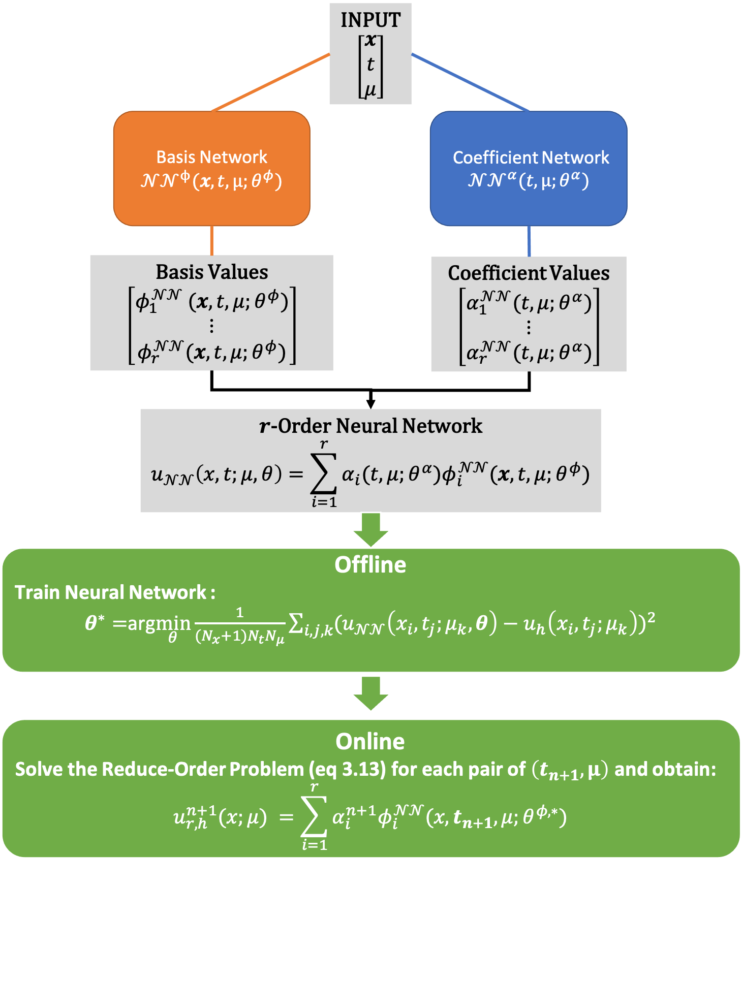
Figure 3.2: The flow chart of the proposed algorithm

4 Numerical experiments

In this section, we demonstrate the performance of the proposed learning-based projection (LP) method by applying it to linear and nonlinear hyperbolic conservation laws in 1D and 2D. Particularly, the 1D and 2D linear advection equation, the 1D and 2D Burgers equation, and the 1D compressible Euler system of gas dynamics are tested. We also compare our method with the standard POD method and the prediction directly provided by the neural network $u_{\mathcal{N}\mathcal{N}}$ in (3.9). Throughout this section, the reduced order solution obtained with the learning-based projection method is referred to as “LP” and the one directly predicted by the neural network $u_{\mathcal{N}\mathcal{N}}$ is referred to as “learning”.

In our numerical experiments, we adopt the feed forward neural network architecture for both ${\mathcal{N}\mathcal{N}}^{\phi}$ and ${\mathcal{N}\mathcal{N}}^{\alpha}$. The activation function is taken as $\tanh$, except for the output layers which are defined as

$${\bf{y}}_{\textrm{output}}=\textrm{softmax}(W{\mathbf{x}})+b,$$ (4.20)

for both the basis and coefficients. Here, $W$ is the weight and $b$ is the bias and $\mathbf{x}$ stands for the output of the previous layer. Among different activation functions of the output layer we have numerically experimented with, softmax outperforms other choices. As pointed out in [30], the softmax activation function introduces $h$-adaptivity to some extent, which may have made the neural network more suitable for the transport problems with local structures. As presented in Section 4.4, the proposed method is not sensitive to the choice of the width and the depth of the hidden layers of the neural network. Unless specified, the neural network ${\mathcal{N}\mathcal{N}}^{\phi}$ has $4$ hidden layers of $25$ neurons per layer and an output layer with $r$ neurons. The neural network ${\mathcal{N}\mathcal{N}}^{\alpha}$ has $3$ hidden layers of $25$ neurons per layer and an output layer with $r$ neurons.

Our code is implemented under the framework of Tensorflow 2.0 [1]. When an implicit time integrator such as backward Euler or Crank-Nicolson method is applied, the associated linear or linearized systems are solved by the GMRES method. If the equation is nonlinear, the Newton’s method will be applied first as an outer loop iterative solver.

4.1 Preliminaries

To set the stage, we start with a 1D scalar hyperbolic conservation law

$$u_{t}+\left(f\left(u\right)\right)_{x}=0,\;x\in[x_{L},x_{R}]$$ (4.21)

with an initial condition and some suitable boundary conditions.

Let $x_{L}=x_{0}<x_{1}\dots<x_{N_{x}}=x_{R}$ be a uniform mesh in space, with $x_{i}=x_{L}+i\Delta x$ and $\Delta x=\frac{x_{R}-x_{L}}{N_{x}}$, and let $\Delta t$ be the time step size. One of the full order models used in our experiments is the following first-order method, that involves the backward Euler method in time and a first-order conservative finite difference method in space:

$$\frac{u_{j}^{n+1}-u^{n}_{j}}{\Delta t}+\frac{f^{n+1}_{j+\frac{1}{2}}-f^{n+1}_{j-\frac{1}{2}}}{\Delta x}=0.$$ (4.22)

Here, $u_{j}^{n}\approx u(x_{j},t_{n})$, $f^{n}_{j+\frac{1}{2}}$ is a numerical flux at $x_{j+\frac{1}{2}}=\frac{x_{j}+x_{j+1}}{2}$, which will be specified later. Boundary conditions are imposed through numerical fluxes. The method in (4.22) can be easily extended to non-uniform meshes, and it can also be interpreted as a finite volume method, with $u_{j}^{n}$ as the element average.

Throughout this section, the $L_{2}$ error and the relative $L_{2}$ error for the solution associated with a test parameter $\mu$ at $t_{n}$ are defined as

$$\mathcal{E}^{n}_{L_{2}}(\mu)=\sqrt{\sum_{j=0}^{N_{x}}(u_{\textrm{reduced},j}^{n}-u_{\textrm{full},j}^{n})^{2}\Delta x},$$ (4.23a)

$$\mathcal{E}^{n}_{\textrm{relative}}(\mu)=\frac{\mathcal{E}^{n}_{L_{2}}(\mu)}{\sqrt{\sum_{j=0}^{N_{x}}(u_{\textrm{full},j}^{n})^{2}\Delta x}},$$ (4.23b)

respectively. The average relative $L_{2}$ error for a test set $\{\mu_{i}\}_{i=1}^{N_{\mu}}$ from $t_{n_{0}}$ to $t_{n_{m}}$ is defined as

$$\mathcal{E}_{\textrm{average}}=\frac{1}{N_{\mu}}\sum_{i=1}^{N_{\mu}}\max_{n_{0}\leq n\leq n_{m}}\left\{\mathcal{E}^{n}_{\textrm{relative}}({\color[rgb]{0,0,0}\mu_{i}})\right\}.$$ (4.24)

The 2D analog of these quantities can be defined similarly.

4.2 1D linear advection equation: learned basis functions

We first consider the 1D linear advection equation of the constant velocity 1:

$$u_{t}+u_{x}=0,$$ (4.25)

with the initial condition

$$u(x,0)=\begin{cases}2,\quad 0.5\leq x\leq 1.5,\\ 0,\quad\text{otherwise.}\end{cases}$$ (4.26)

The computational domain is $[0,5]$, and it is partitioned with a uniform mesh with $\Delta x=0.01$. The time step size is taken as $\Delta t=\Delta x$. We use the exact solution from $t=[0,0.75]$ to train the neural network with the reduced order $r=3$. The purpose of this example is to test whether the proposed method is able to capture the underlying $t$-dependent transformation.

In Figure 4.3, we present the learned basis functions at three different times obtained offline. We observe that, as time evolves, all three basis functions propagate from the left to the right with a wave speed approximately $1$. This qualitatively verifies that the proposed LP method is able to capture the underlying physics. In Figure 4.4, we further qualitatively measure the difference between the learned basis functions and shifted initial basis functions with wave speed $1$. As time evolves, the difference will be larger.

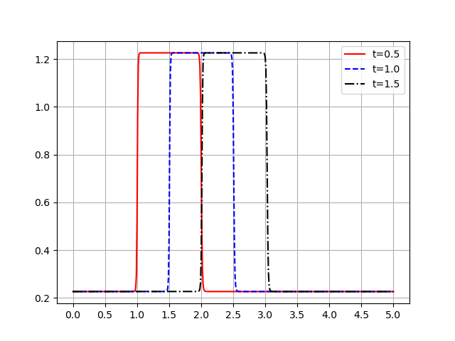
(a) Basis function 1

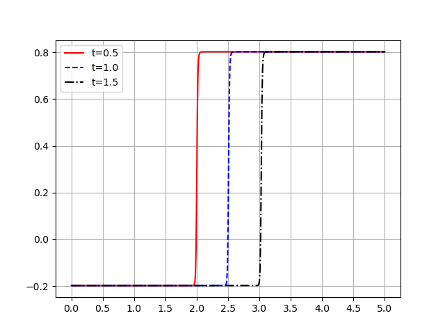
(b) Basis function 2

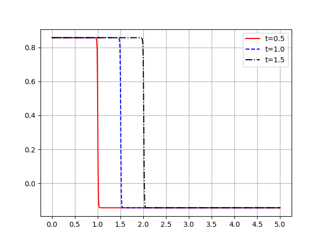
(c) Basis function 3

Figure 4.3: The learned basis functions ${\phi}^{\mathcal{N}\mathcal{N}}_{i}$ for $i=1,2,3$ at different times for the linear advection equation in Section 4.2.

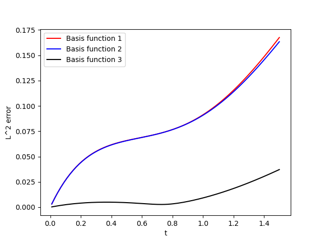
Figure 4.4: The difference between the learned basis functions and the shifted initial basis functions for the linear advection equation in Section 4.2.

4.3 1D linear advection equation with a moving mesh method

The aim of this example is to show the flexibility and the effectiveness of our method to couple with a full order moving mesh method.

We consider the same linear advection equation as in Section 4.2, but with a slightly different initial condition

$$u(x,0)=\begin{cases}2,\quad 0.6<x<1.4,\\ 0,\quad\text{otherwise.}\end{cases}$$ (4.27)

We use a non-uniform moving mesh: $0=x_{0}(t)<x_{1}(t)<\dots<x_{N_{x}}(t)=5.0$, with $N_{x}=1000$. Define $h_{\textrm{coarse}}=\frac{1}{125}$ and $h_{\textrm{refine}}=\frac{1}{500}.$ The grid point at time $t$, namely, $x_{i}(t)$ ($1\leq i\leq N_{x}-1$), satisfies

$$x_{i}(t)=\begin{cases}x_{i-1}(t)+h_{\textrm{refine}},\quad\text{if\;}0.5+t\leq x_{i-1}(t)\leq 1.5+t,\\ x_{i-1}(t)+h_{\textrm{coarse}},\quad\text{otherwise}.\end{cases}$$ (4.28)

This mesh moves with the underlying wave speed and is always more refined near the discontinuity of the solution. With this moving mesh, the first order upwind finite volume method with $f^{n}_{j+\frac{1}{2}}=u_{j}^{n}$ is applied in space, together with the backward Euler method in time and the time step size $\Delta t=h_{\textrm{coarse}}$. Before marching to the next time step, an extra key step of a moving mesh method is to interpolate the solution from the mesh at $t^{n-1}$ to the mesh at $t^{n}$. In our simulation, we follow the Step 2 of the moving mesh algorithm [56] to do this interpolation. When our LP method is applied, we use the same interpolation subroutine to interpolate predicted solution from the old mesh to the new mesh. Extra cost reduction can be done in this step, and this is not explored here.

The training set is the snapshot solutions for $t\in[0,0.75]$ ($95$ time snapshots), and we will predict the solution from $t=0.75$ to $t=1.5$. With the moving mesh, each solution snapshot corresponds to a different mesh. As a result, interpolation of basis functions from different meshes [20] or extra refinement and re-computation with a more refined common mesh [64, 65] may be needed for the standard POD or RB method. Our neural networks take $x$, $t$ as inputs in a mesh-free manner, and hence do not need additional treatments to work with basis functions associated with different meshes. Here, we only present results of the pure learning based method and the LP method.

In Figure 4.5, we present the predicted solution at $t=1.5$ and the error history with $r=15$. Both the learning based and the LP methods match the full order solution well, and the error of the LP method is overall smaller. From Figure 6(a) (resp. Figures 6(c)- 6(d)) with $r=5,10,15,20,25$, we further observe that the LP method leads to smaller average absolute (resp. relative) errors than the learning based method.

Finally we want to compare the computational efficiency between the LP method and the full order method. As it is mentioned, both methods share the same subroutine to interpolate a computed solution from one mesh to another. The total number of the time steps are also the same for both methods. Therefore in Figure 6(b), we only show the relative average CPU time (i.e. relative to that of the full order method) to invert the linear system for one step time marching. With $N_{x}=1000$, it is observed that with $5$ to $25$ basis functions, it takes the LP method around $36\%$ of the time of the full order method to invert the resulting linear system.

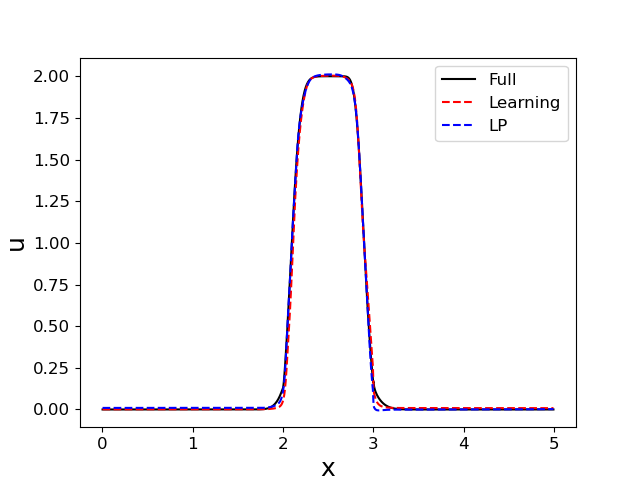
(a) Predicted solutions with 15 reduced basis functions

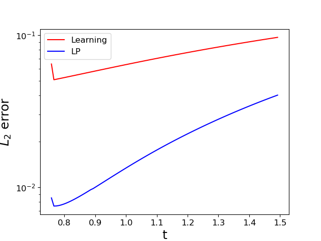
(b) Error history with 15 reduced basis functions

Figure 4.5: Predicted solutions at $t=1.5$ (left) and the error history (right) with 15 reduced basis functions for the moving mesh test in Section 4.3.

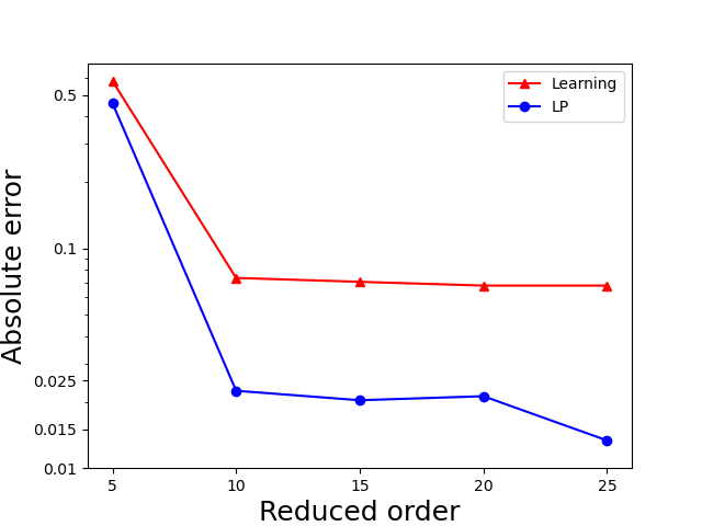
(a) Average absolute error

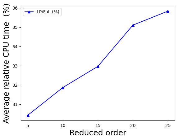
(b) Average relative CPU time to invert the linear system for one step time marching

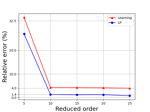
(c) Average relative error

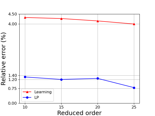
(d) Average relative error (zoomed-in)

Figure 4.6: Average absolute/relative error and average relative CPU time to invert the linear system for one step time marching, versus the reduced order $r$ for the moving mesh test in Section 4.3.

4.4 2D linear advection equation

In this example, we consider a 2D linear advection equation:

$$u_{t}+b\cdot\nabla u=0,\quad(x,y)\in[0,1]\times[0,1]$$ (4.29)

with $b=(1.0,2.0)^{T}$ and the zero initial condition. The boundary condition is given at the inflow boundary $\Gamma_{\textrm{inflow}}=\{(x,y)\in[0,1]\times[0,1]:xy=0\}$ as below,

$$u(x,y)|_{(x,y)\in\Gamma_{\textrm{inflow}}}=\begin{cases}1+\cos(8\pi x),\quad 0.125<x<0.625,\\ 0,\quad\text{otherwise}.\end{cases}$$ (4.30)

The computational domain is partitioned by a triangular mesh $\mathcal{T}_{h}=\{\mathcal{T}_{i}\}_{i=1}^{N_{x}}$. In space, we apply the upwind discontinuous Galerkin (DG) method: seeking $u_{h}\in V_{h}:=\bigoplus_{\mathcal{T}_{i}\in\mathcal{T}_{h}}\mathcal{P}^{1}(\mathcal{T}_{i})$ satisfying

$$\sum_{\mathcal{T}_{i}\in\mathcal{T}_{h}}\left(\int_{\mathcal{T}_{i}}\partial_{t}u_{h}v-(b\cdot\nabla v)u_{h}dx+\int_{\partial\mathcal{T}_{i}}\widehat{b\cdot\mathbf{n}_{i}u_{h}}vds\right)=0,\quad\forall v\in V_{h}.$$ (4.31)

Here, $\mathcal{P}^{1}(\mathcal{T}_{i})$ is the linear polynomial space on $\mathcal{T}_{i}$, $\mathbf{n}_{i}$ is the outward unit normal of $\mathcal{T}_{i}$ along its boundary $\partial\mathcal{T}_{i}$, and $\widehat{b\cdot\mathbf{n}_{i}u_{h}}$ is the upwind flux that is based on the upwind mechanism and defined as $\widehat{b\cdot\mathbf{n}_{i}u_{h}}=b\cdot\mathbf{n}_{i}\textrm{lim}_{\epsilon\rightarrow 0+}u_{h}(x-(b\cdot\mathbf{n}_{i})\mathbf{n}_{i}\epsilon).$ In time, we apply the trapezoidal method that is second order accurate. The DG code is implemented with the python interface of the c++ finite element library NGSolve [52].

The mesh in our test consists of $N_{x}=3710$ elements with the maximal edge length $h_{\textrm{max}}=0.025$ (see Figure 7(a)), and the time step size is set as $\Delta t=\frac{0.5h_{\textrm{max}}}{\|b\|_{2}}$. The training data is the nodal values of the full order solution for $t\in[0,0.2]$ ($37$ time snapshots) and we predict the solution from $t=0.2$ to $t=0.4$. We find it much easier to train the neural network using nodal values instead of modal coefficients as the degrees of freedom. Since NGSolve implements the DG method based on a modal basis instead of a nodal basis, this leads to extra cost to covert between the nodal values and modal coefficients of the solution.

In Figure 4.7, we present the full order solution, the LP and POD solutions with $r=10$ at $t=0.4$, as well as the error in the LP solution. It is clear that the LP method matches the full order solution much better than the POD method. In Figure 4.8, we present the absolute error at $t=0.4$ for different methods and the relative CPU time of the LP method. We observe that the LP method always leads to the smallest error, and it only needs less than $25\%$ CPU time of the full order solve even with the extra online overhead to convert nodal values to modal coefficients.

We also use this example to illustrate that the proposed method is relatively insensitive to the width and the depth of the hidden layer of the neural network. In Figure 4.9, we present the final value of the loss function and the prediction error of the trained neural network at $t=0.2$ with different width and depth of the hidden layer. The two neural networks that represent the basis and the coefficients share the same width and the depth. These neural networks are also trained with the solution snapshots for $t\in[0,2]$, and the learning rate is $10^{-3}$ and the number of epochs is $30$. For each pair of depth and width, the value of the loss function and the prediction error are the average value of $5$ different random initialization of the neural network. We observe that when the depth is not less than $2$ and the width is not less than $10$, the final value of the loss function and the prediction error of the trained neural network at $t=0.2$ do not change much with respective to the depth and the width.

The last test for this example is to investigate the relation between the cost to generate the reduced basis online and the architecture of the neural networks. In Figure 4.10, we compute the average CPU time of $100$ runs to generate reduced basis for $t=0.4$ and $r=10$. In 10(a), we fix the depth of the hidden layer as $3$ and vary the width of the hidden layer. In 10(b), we fix the width of the hidden layer as $25$ and vary the depth. We observe that the computational cost of generating $10$ reduced basis functions is roughly proportional to the width and the depth of the hidden layer. We also would like to point out that, as to be shown in Section 4.5, the computational time of generating the basis will be less than solving the reduced order projection equation when the mesh is refined enough.

(a) Full order solution

(b) LP solution with $10$ basis functions

(c) Error of the LP method with $10$ basis functions

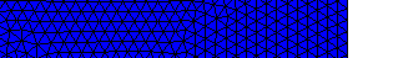
(d) POD solution with $10$ basis functions

Figure 4.7: The full order solution, the LP solution and its error with 10 basis functions, and the POD solution with 10 basis functions, all at $t=0.4$ for the 2D linear advection equation in Section 4.4.

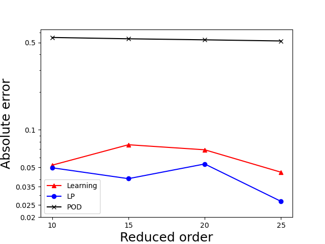
(a) Absolute error at $t=0.4$

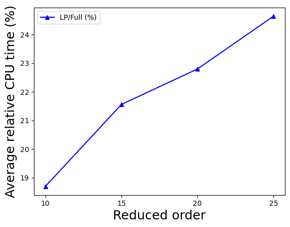
(b) Average relative CPU time

Figure 4.8: The absolute error at $t=0.4$ and the average relative CPU time for the 2D linear advection equation in Section 4.4.

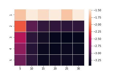
(a) Final value of the loss function of trained neural network

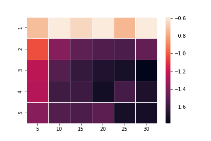
(b) The $L_{2}$ prediction error of the trained neural network at $t=0.2$ under $\log$-scale

Figure 4.9: $x$-axis: width of the hidden layers; $y$-axis: depth of the hideen layers; color: the value of the loss function/error under log scale.

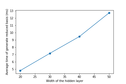
(a) Depth of the hidden layer, $3$

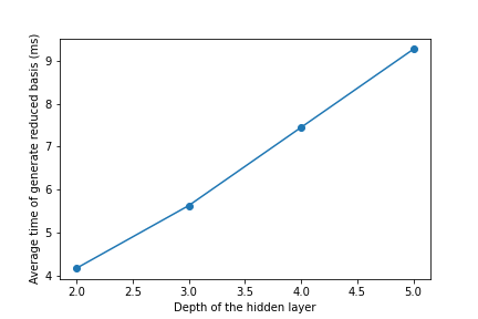
(b) Width of the hidden layer, $25$

Figure 4.10: $x$-axis: width/depth of the hidden layers; $y$-axis: average CPU time to generate $10$ reduced basis functions online.

4.5 1D linear advection equation with $(x,\mu)$-dependent inhomogeneous media

In this example, we consider the following 1D linear advection equation

$$u_{t}+(c(x;\mu)u)_{x}=0$$ (4.32)

in an inhomogeneous media where the propagation speed $c(x,\mu)$ is $(x,\mu)$-dependent, given as

$$c(x;\mu)=1.25+\mu_{1}\sin(\mu_{2}\pi x),\quad{\color[rgb]{0,0,0}\mu=(\mu_{1},\mu_{2})}\in X_{\mathcal{P}}=[0,0.5]\times[2,4].$$ (4.33)

The initial condition is

$$u(x,0)=\begin{cases}0.5+0.5\cos(5\pi(x-0.25)),\quad 0.05\leq x\leq 0.45,\\ 0,\quad\text{otherwise{\color[rgb]{0,0,0},}}\end{cases}$$ (4.34)

together with the zero boundary conditions. The spatial computational domain is $[0,2.5]$, and a uniform mesh with $500$ elements is used. To control the numerical dissipation of the full order model, we use the second-order Crank-Nicolson time discretization, and the numerical flux is chosen as an upwind-biased flux:

$$f^{n}_{j+\frac{1}{2}}=\frac{3}{4}c_{j}u_{j}^{n}+\frac{1}{4}c_{j+1}u_{j+1}^{n}$$ (4.35)

with $c_{j}=c(x_{j};\mu)>0$. The time step size is $\Delta t={2\Delta x}$.

Associated with the model parameter $\mu=(\mu_{1},\mu_{2})$, the training set is taken to be $\{\mu_{1}^{(i)}=\frac{i}{20}\}_{i=0}^{10}\times\{\mu_{2}^{(j)}=2+\frac{j}{10}\}_{j=0}^{20}$, and the testing set is constituted by $20$ pairs of $(\mu_{1},\mu_{2})$ randomly sampled from a uniform distribution on the parameter space $X_{\mathcal{P}}$. For both the training and the testing, $t\in[0,1]$ ($231\times 101$ time snapshots) is considered.

In Figure 4.11, we report the average relative testing error of the proposed LP method, the learning method, and the standard POD method versus the reduced order $r$. We observe that the LP method consistently entails the least error for varied $r$. When $r=25$, the error of the LP method is smaller than $0.3\%$. Possibly due to the overfitting, the error of the pure learning-based method does not decay as the number of basis functions increases. The projection step in the online stage reduces the generalization error dramatically, as the PDE information is utilized through this step.

For the testing sample $(\mu_{1},\mu_{2})=(0.23,3.56)$, we present in Figure 4.12 the solutions with different reduced order $r=15,25$ at $t=2$. With $15$ basis functions, the LP solution matches the full order solution better than the POD method, though some non-physical oscillation exists. Additional study can be found in Appendix A to understand the origin of the oscillation. With $25$ basis functions, the LP solution visually coincides with the full order solution.

Our next test aims at showing the flexibility of the LP method when the online spatial meshes are different from the offline ones. Our method avoids extra efforts which are needed by conventional projection based ROMs to accomplish similar tasks [20, 64, 65]. Using the neural network trained with data generated on a uniform mesh with $N_{x}^{\textrm{off}}=500$ spatial elements offline, we evaluate basis function values on uniform meshes with different $N_{x}^{\textrm{on}}$ in the online computation. The relative error for different grid resolutions online with $r=20$ is presented in the left picture of Figure 4.13, and it is reasonably small. In the right picture of Figure 4.13, we present the predicted solution at $\mu=(0.23,3.56)$ and $t=1$ with $N_{x}^{\textrm{on}}=2500$. The full order solution with $N_{x}^{\textrm{off}}=500$ is more dissipative than the full order solution with $N_{x}^{\textrm{on}}=2500$, but the LP solution still matches the full order solution with $N_{x}^{\textrm{on}}=2500$ well, while the pure learning-based method provides a more dissipative solution compared with the full order solution.

The final test we carry out is intended to examine the computational efficiency. In Figure 4.14, for the test sample $(\mu_{1},\mu_{2})=(0.23,3.56)$, we compare the CPU time of the one step online computation of the LP method with $20$ basis functions and that of the full order model for different grid resolutions online. We also compare the times for basis evaluation in (3.14) and for solving the projection equation (3.15) during the online stage of the LP method (see Algorithm 1). For different resolutions online ($N_{x}^{\textrm{on}}$), the reduced-order basis is always trained with $N_{x}^{\textrm{off}}=500$ elements in the offline stage, and the solutions predicted by our method always visually match the full order solution reasonably well. As $N_{x}^{\textrm{on}}$ grows, the CPU time of the basis evaluation grows much slower compared with that for solving the projection equation. For small $N_{x}^{\textrm{on}}$, the ROM spends most of the time on the basis generation. As $N_{x}^{\textrm{on}}$ grows, the computational time of the full order model grows much faster than that of the proposed LP method.

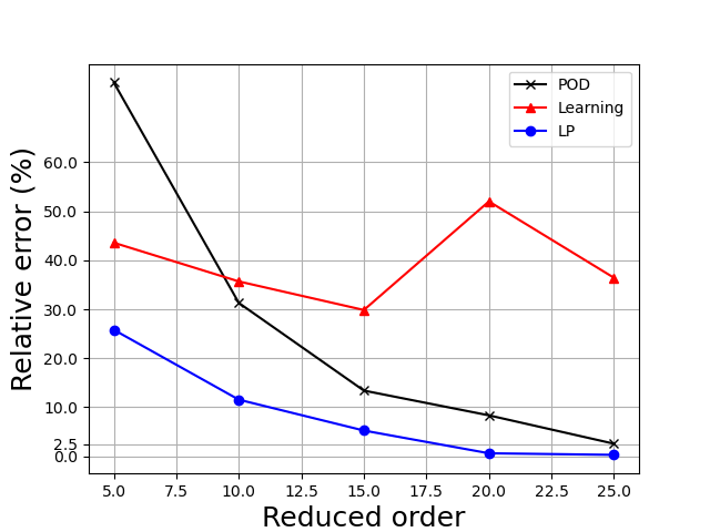
(a) Average relative error

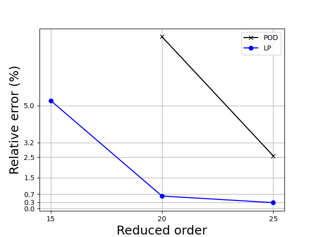
(b) Zoomed-in picture

Figure 4.11: $x$-axis: reduced order $r$; $y$-axis: the average relative error for the test set of the linear advection equation with $(x,\mu)$-dependent inhomogeneous media in 4.5.

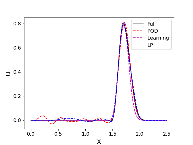
(a) $15$ basis functions

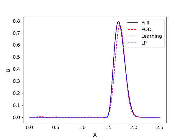
(b) $25$ basis functions

Figure 4.12: Predicted solutions of the linear advection equation with $(x,\mu)$-dependent inhomogeneous media in Section 4.5 at $(\mu_{1},\mu_{2})=(0.23,3.56)$ and $t=1$.

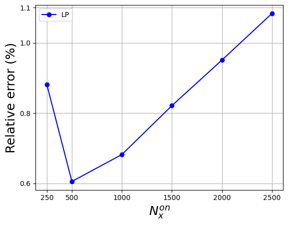
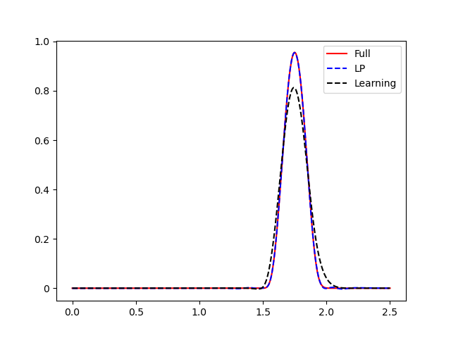
Figure 4.13: Linear advection equation with $(x,\mu)$-dependent inhomogeneous media in Section 4.5. Left: mean relative error of the test set for different online grid resolutions ($N_{x}^{\textrm{on}}$). Right: predicted solution at $\mu=(0.23,3.56)$ and $t=1$ with online mesh $N_{x}^{\textrm{on}}=2500$. $20$ basis functions are used and are trained offline with data subject to constant resolution ($N_{x}^{\textrm{off}}=500$).

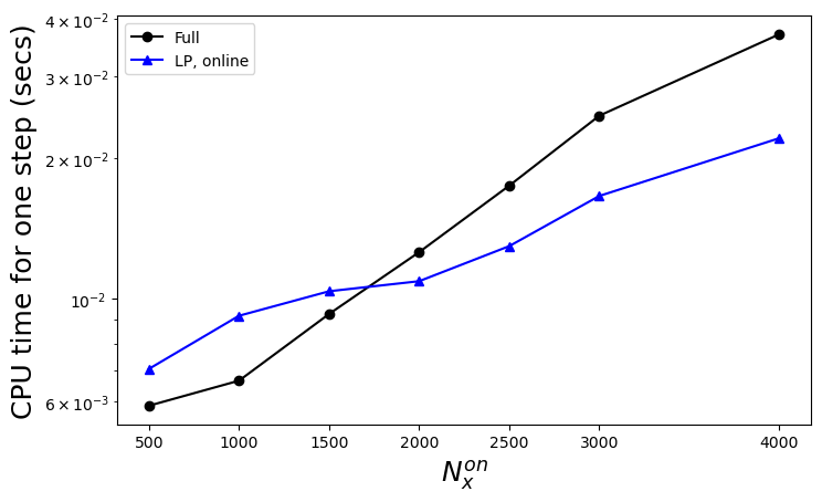
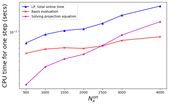
Figure 4.14: The average CPU time for one time step as a function of different online resolution $N_{x}^{\textrm{on}}$. Left: full order model v.s. the online computation of the LP method. Right: online basis evaluation, the online solve of projection equation of the LP method and the total time of the online computation of the LP method.

4.6 1D Burgers Equation

We consider the Burgers equation:

$$u_{t}+\left(\frac{1}{2}u^{2}\right)_{x}=0,$$ (4.36)

and perform two sets of experiments. In the first one, we consider a Riemann problem with a parameter in the initial data, and the solutions will be predicted for a test set of parameter and for future times. In the second experiment, we start with a smooth initial profile, and shock discontinuity will form later. We will predict the solutions at future times based on the full order solution on $[0,t_{0}]$, over which the shock structure may or may not have been “seen” by the offline training algorithm. The first order method in (4.22) will be applied, with the numerical flux chosen as:

$$f_{j+\frac{1}{2}}^{n}:=\frac{1}{2}\left(f(u_{j+1}^{n})+f(u_{j}^{n})\right)-\frac{\Delta x}{2\Delta t}(u_{j+1}^{n}-u_{j}^{n}).$$ (4.37)

4.6.1 Parameter-dependent Riemann problem

We consider the computational domain $[0,8]$ with a parameter-dependent initial condition:

$$u(x,0)=\begin{cases}1.+\mu,\quad{\color[rgb]{0,0,0}x\in[0.5,0.75]},\\ 0.,\quad\text{otherwise.}\end{cases}$$ (4.38)

Here, $\mu\in X_{\mathcal{P}}=[0,1]$. The solution has a rarefaction fan and a moving shock. We use a uniform mesh with $N_{x}=400$. The time step size is set to be $\Delta t=\Delta x$.

The training set is taken as $\{0,0.1,0.2,\dots,1\}\subset X_{\mathcal{P}}$ with $0\leq t\leq 0.25$ ($11\times 101$ snapshots). The test set is taken as $\{0.05\pm 0.01,0.15\pm 0.01,\dots,0.95\pm 0.01\}\subset X_{\mathcal{P}}$, and we predict the solution from $t=0$ to $t=0.5$. In the offline stage of this problem, we train the neural network with $150$ epochs.

In Figure 4.15, the average relative errors for the test set are presented corresponding to different reduced order $r$. Overall, we observe that for both the POD method and the LP method, the error decays as $r$ grows. However, this is not the case for the purely learning-based method. Moreover, the error of the LP method is much smaller than that of the other two methods.

In Figure 4.16, we present the predicted solutions for $\mu=0.76$ at $t=0.5$ with $r=15,25$. We observe that the LP method performs better than the other two methods in matching the full order solution, especially in capturing the shock location. There are small oscillations near the shock location in the LP solution .

In Figure 4.17, we present the time evolution of the $L_{2}$ error in prediction for $\mu=0.76$ under the $log$-scale with $r=15$ and $25$. Among the LP method, the learning method, and the POD method, the LP method displays the slowest growth in its error over time. When $r=25$, we observe that the error of the POD method is smaller than that of the LP method for $t\leq 0.25$, then it grows dramatically fast and becomes much larger than the LP method. The reason why the POD method becomes much worse after $t=0.25$ is that we only have the training data for $t\leq 0.25$ in the offline stage. The LP method shows its advantages in providing more accurate and stable long time prediction.

In Figure 4.18, we present the relative CPU time with different number of mesh elements in the online stage $N_{x}^{\textrm{on}}$ and $r=20$. The neural network is trained with $N_{x}^{\textrm{off}}=400$. When the mesh is refined enough, the LP method does lead to smaller computational time compared with a full order solver. However, when the mesh is refined with larger $N_{x}^{\textrm{on}}$, the LP method produces more numerical oscillations. It becomes important on much refined meshes to control non-physical oscillations of reduced order solutions and to improve numerical stability.

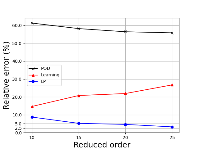
(a) Average relative error

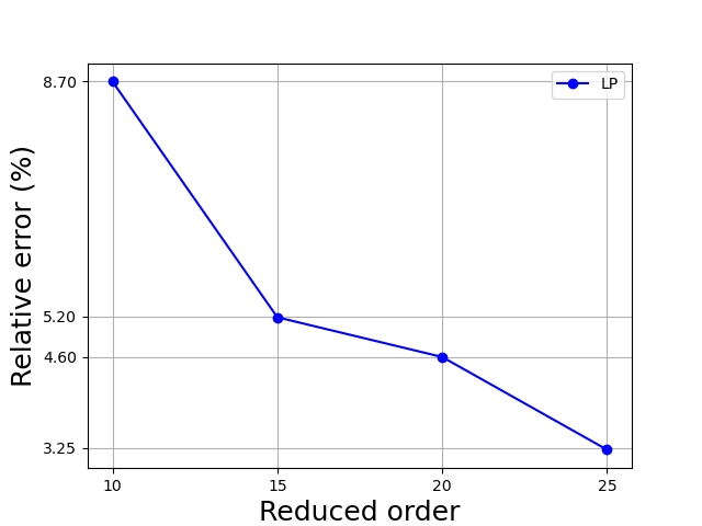
(b) Zoomed-in picture

Figure 4.15: $x$-axis: reduced order $r$; $y$-axis: the average relative error for the test set of the Burgers equation (parameter dependent initial profile) in Section 4.6.1.

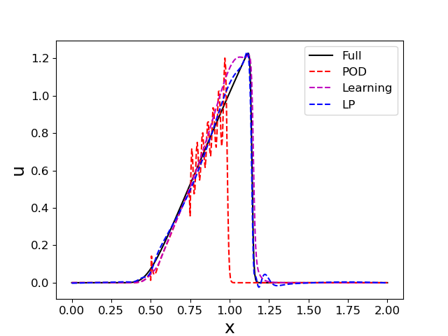
(a) $15$ basis functions

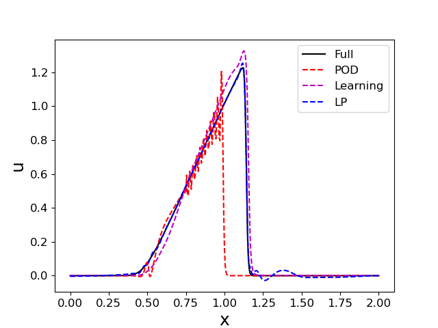
(b) $25$ basis functions

Figure 4.16: Predicted solutions for the Burgers equation (parameter dependent initial profile) in Section 4.6.1 with $\mu=0.76$ and $t=0.5$.

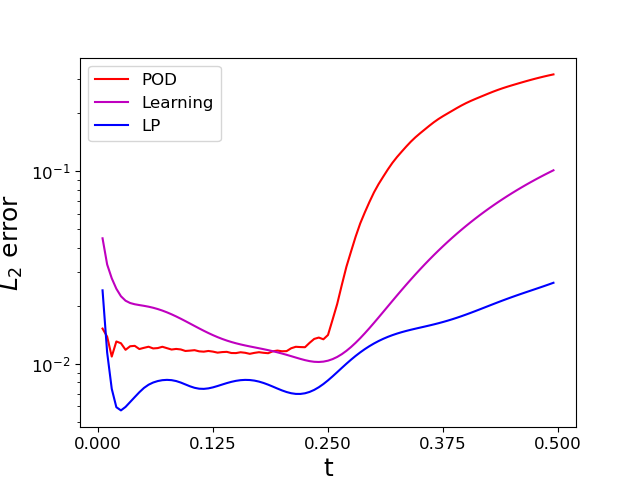
(a) $15$ basis functions

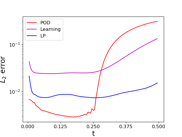
(b) $25$ basis functions

Figure 4.17: The time evolution of the prediction error history for the Burgers equation (parameter dependent initial profile) in Section 4.6.1 with $\mu=0.76$.

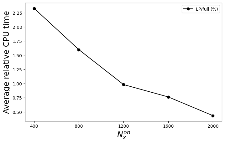
Figure 4.18: Relative computational time with different resolutions in the online stage.

4.6.2 Future prediction with smooth initial profile and shock formation

We consider the computational domain $[-1,1]$ and the following initial condition

$$u(x,0)=\frac{1}{4}+\frac{1}{2}\sin(\pi x)$$ (4.39)

with periodic boundary conditions. Though with a smooth initial profile, a shock will form at $t=t_{\star}=\frac{2}{{\pi}}$ and then moves as time evolves. We use a uniform mesh with $N_{x}=400$ and the time step size $\Delta t=0.25\Delta x$.

We consider two training sets, which are the full order numerical solutions for $t\in[0,t_{0}]$, with $t_{0}=1.1$ (when shock has formed with $881$ snapshots in the training set) and $t_{0}=0.6$ (when shock has not formed yet with $481$ snapshots in the training set), respectively. We predict the solution from $t=t_{0}$ to $t=1.6$. The neural network is trained with $100$ epochs. It is expected that the experiment with the second training data which has not “seen” any shock to be more challenging in future prediction.

In Figure 4.19, we present the predicted reduced-order solutions at $t=1.6$. We observe that, with both $t_{0}=1.1$ and $t_{0}=0.6$, the solutions by the LP method always match the full order solution the best. Even though the training data corresponding to $t\in[0,0.6]$ does not include any solutions with shock features, the LP method captures the correct shock location in the predicted solutions. Besides, with the training data from $t\in[0,0.6]$, the results of the LP method are relatively more oscillatory. The numerical oscillation is further suppressed with an increase of the reduced order $r$.

In Figure 4.20, we present the largest relative prediction error from $t=t_{0}$ to $t=1.6$ when the ROM is trained with the data sampled from $t=[0,t_{0}]$ for $t_{0}=1.1$ or $t_{0}=0.6$ versus the reduced order $r$. For both cases, the LP method always has the smallest relative error. When trained with $t_{0}=1.1$, the relative error of the LP method is approximately $0.71\%$ with $20$ basis functions and $0.15\%$ with 25 basis functions. For the same number of reduced basis, the relative error of the LP method trained with $t_{0}=1.1$ is smaller than that with $t_{0}=0.6$.

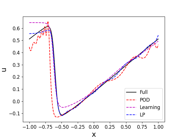
(a) 15 basis functions; training data: $t\in[0,1.1]$

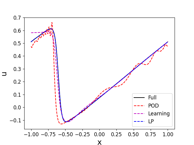
(b) 25 basis functions; training data: $t\in[0,1.1]$

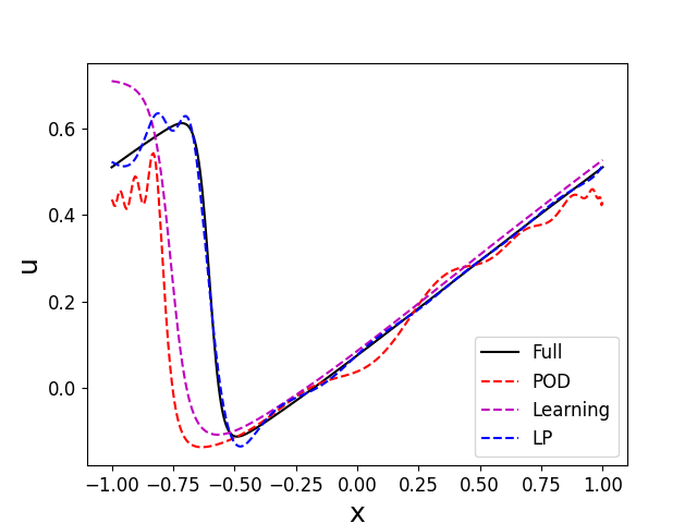
(c) 15 basis functions; training data: $t\in[0,0.6]$

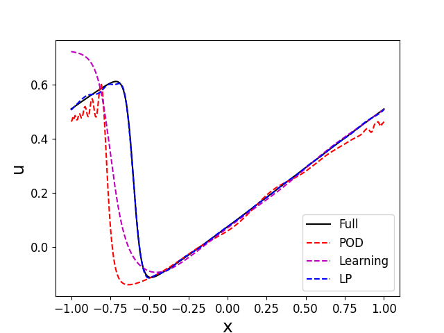
(d) 25 basis functions; training data: $t\in[0,0.6]$

Figure 4.19: Predicted solutions of the Burgers equation with smooth initial profile and shock formation in Section 4.6.2 at $t=1.6$.

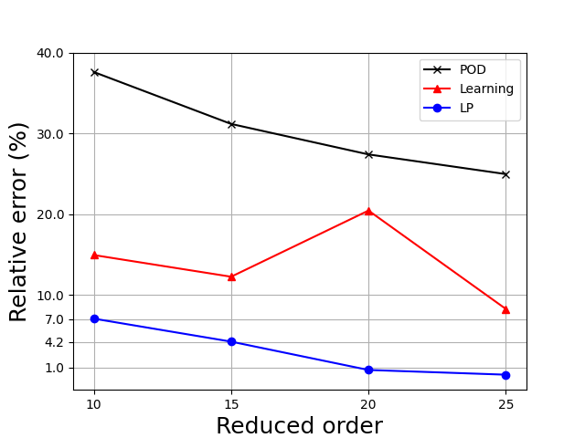
(a) Comparison between pure learning, POD and the LP method, training data: $t\in[0,1.1]$

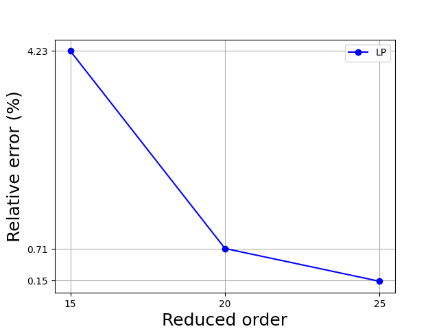
(b) Zoomed-in picture, training data: $t\in[0,1.1]$

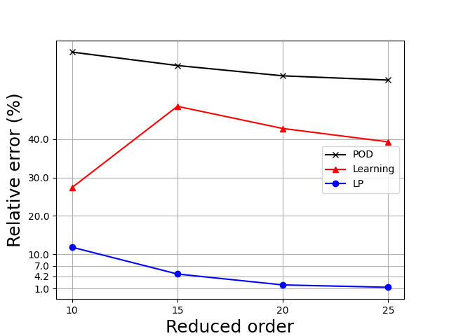
(c) Comparison between pure learning, POD and the LP method, training data: $t\in[0,0.6]$

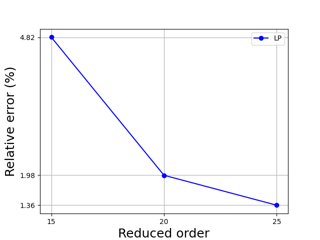
(d) Zoomed-in picture, training data: $t\in[0,0.6]$

Figure 4.20: $x$-axis: reduced order $r$; $y$-axis: the largest relative prediction error for the Burgers equation with smooth initial profile and shock formation in Section 4.6.2.

4.7 2D Burgers equation

We consider a 2D Burgers equation:

$$u_{t}+\nabla\cdot\mathbf{F}(u)=0,\quad(x,y)\in[-1,1]\times[-1,1],$$ (4.40)

with $\mathbf{F}(u)=(\frac{u^{2}}{2},\frac{u^{2}}{2})^{T}$ and the following initial condition (also see 21(c)),

$$u(x,0)=\begin{cases}\sin\left(\pi(0.5-\sqrt{x^{2}+y^{2}})\right),\quad\sqrt{x^{2}+y^{2}}\leq 0.5,\\ 0,\quad\text{otherwise}.\end{cases}$$ (4.41)

The computational domain is partitioned by a triangular mesh $\mathcal{T}_{h}=\{\mathcal{T}_{i}\}_{i=1}^{N_{x}}$, with $N_{x}=5822$ and the maximal edge length $h_{\textrm{max}}=0.04$. In space, we apply a DG method: seeking $u_{h}\in V_{h}:=\bigoplus_{\mathcal{T}_{i}\in\mathcal{T}_{h}}\mathcal{P}^{1}(\mathcal{T}_{i})$ satisfying

$$\sum_{\mathcal{T}_{i}\in\mathcal{T}_{h}}\left(\int_{\mathcal{T}_{i}}(\partial_{t}u_{h}v-\mathbf{F}(u_{h})\cdot\nabla v)dx+\int_{\partial\mathcal{T}_{i}}\widehat{\mathbf{F}\cdot\mathbf{n}_{i}}vds\right)=0,\quad\forall v\in V_{h}.$$ (4.42)

Here we use the local Lax-Fridriches flux

$$\widehat{\mathbf{F}\cdot\mathbf{n}_{i}}=\frac{(\mathbf{F}(u_{h}^{+})+\mathbf{F}({u_{h}}^{-})}{2}\cdot\mathbf{n}_{i}+\frac{\lambda_{i}}{2}(u_{h}^{+}-u_{h}^{-}),$$ (4.43)

where $\mathbf{n}_{i}$ is the outward unit normal of $\mathcal{T}_{i}$ along its boundary $\partial\mathcal{T}_{i}$, $u_{h}^{+}$ is the value of $u_{h}$ on $\partial{\mathcal{T}_{i}}$ from the interior of $\mathcal{T}_{i}$, $u_{h}^{-}$ is the value of $u_{h}$ on $\partial{\mathcal{T}_{i}}$ from the neighboring element of $\mathcal{T}_{i}$ sharing the same edge, and $\lambda_{i}=|[1,1]^{T}\cdot\mathbf{n}_{i}|\max(|u_{h}^{+}|,|u_{h}^{-}|)$. In time, we apply the forward Euler method with the time step size $\Delta t=0.001$. To stabilize both the full and reduced order solvers, an artificial viscosity term $\frac{1}{8}h\Delta u$ is added to the equation in an element-wise fashion (with $h|_{\mathcal{T}_{i}}$ as the element diameter), and is discretized by the symmetric interior penalty method [63]. The training data is the solution snapshots from $t=0.2$ to $t=0.35$ ($151$ time snapshots), and we predict the solution at $t=0.42$. The coefficient neural network has $2$ hidden layers with $25$ neurons per layer, and the basis neural network has $3$ layers with $25$ neurons per layer. In Figure 4.21, we present the full order solution with and without artificial viscosity. Without artificial viscosity, one can see the non-physical oscillations near the wave front in the full order solution, and the LP method produces even more oscillatory solutions.

As mentioned before, there will be no saving of computational cost with the forward Euler time integrator. The purpose of this test is to check whether the neural network is capable of capturing the underlying low-rank structure in 2D nonlinear hyperbolic problems. The reduced order solutions with 10 basis functions at $t=0.42$ are presented in Figure 4.22, all with the artificial viscosity strategy applied. The LP method and the pure learning-based method match the full order solution (in Figure 22(a)) reasonably well, while the POD method with the same number of basis functions fails to capture the solution structure when going beyond the training set. In Figure 4.23, the absolute errors at $t=0.42$ versus the reduced order $r$ are presented for the LP and the pure learning methods. The errors of the two method are close to each other, but the online stage of the pure learning method is faster, as it only needs function evaluation.

(a) Full order solution without artificial viscosity

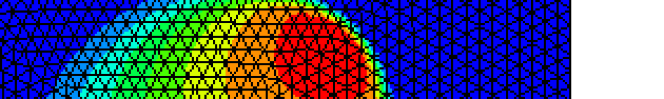
(b) Full order solution with artificial viscosity

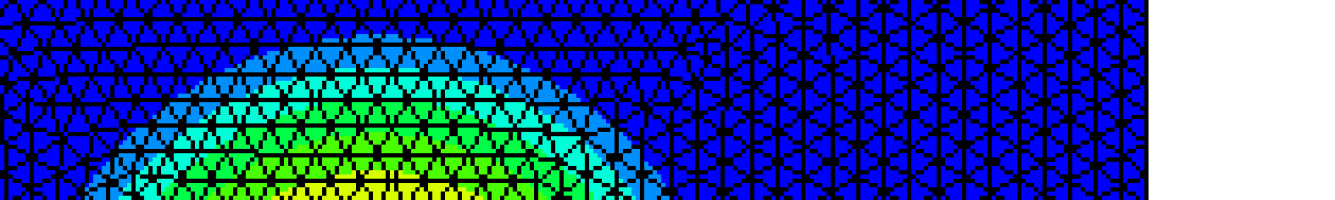
(c) Initial condition

Figure 4.21: Initial condition, and full order solutions with and without artificial viscosity at $t=0.42$ for the 2D Burgers equation in Section 4.7.

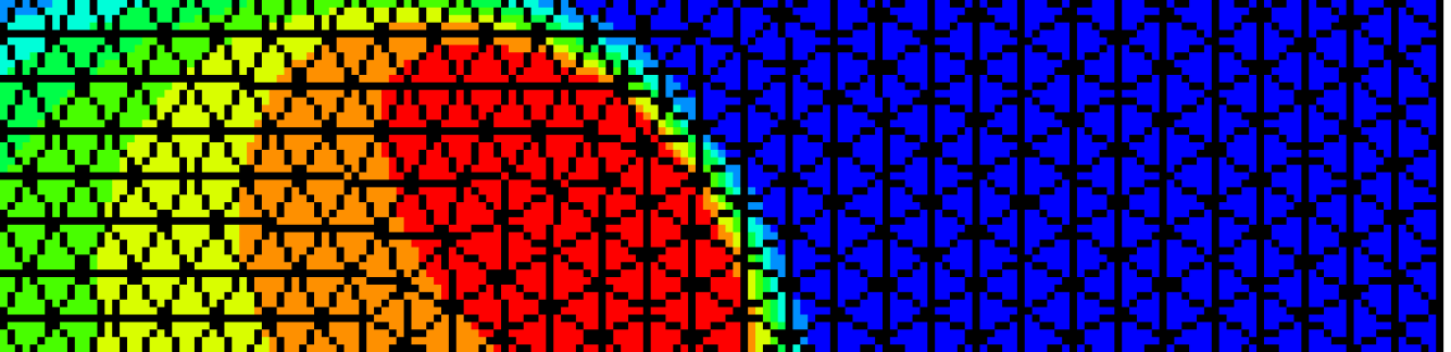
(a) LP solution with 10 basis functions

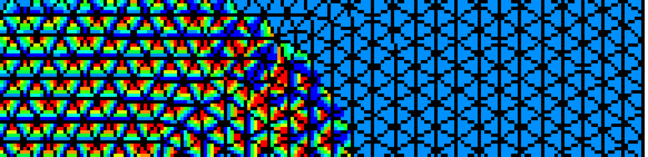
(b) POD solution with $10$ basis functions

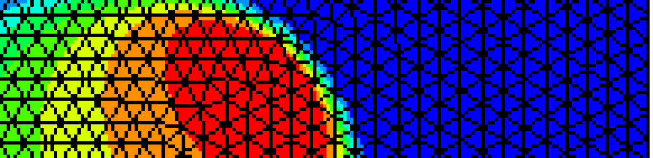
(c) Learning solution with 10 basis functions

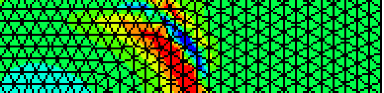
(d) Error of the LP method with $10$ basis functions

Figure 4.22: Full order and reduced order solutions and error at $t=0.42$ for the 2D Burgers equation in Section 4.7.

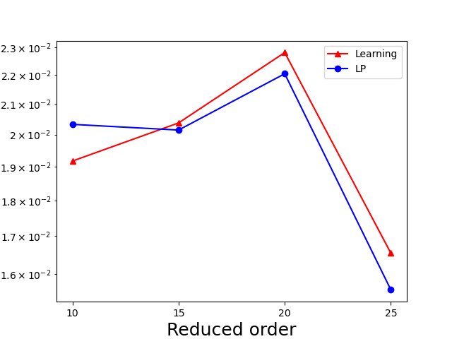
(a) Absolute error at $t=0.42$

Figure 4.23: The absolute error at $t=0.42$ for the 2D Bureges equation in Section 4.7.

4.8 Compressible Euler system

Finally we apply the proposed LP method to the 1D compressible Euler system of gas dynamics:

$$\begin{cases}&\rho_{t}+(\rho u)_{x}=0,\\ &(\rho u)_{t}+(\rho u^{2}+p)_{x}=0,\\ &E_{t}+\left(u(E+p)\right)_{x}=0.\end{cases}$$ (4.44)

Here $\rho,u,p$ are the density, velocity, pressure, respectively, with the total energy $E=\frac{p}{\gamma-1}+\frac{1}{2}\rho u^{2}$ and $\gamma=3$ for the ideal gas. We consider the Sod’s shock tube problem, with the initial conditions:

$$\rho(x,0)=\begin{cases}1.0,\quad x<0,\\ 0.125,\quad x\geq 0,\end{cases}\quad u(x,0)=0.0,\quad p(x,0)=\begin{cases}1.0,\quad x<0,\\ 0.1,\quad x\geq 0.\end{cases}$$ (4.45)

For this example, the full order method is based on the fifth-order WENO finite difference method with the Lax-Friedrichs flux [25] and the explicit third order strong stability preserving Runge-Kutta method [53]. With an explicit time integrator applied, the LP method will not reduce the computational time. We want to use this example to demonstrate that the proposed method can capture the hidden low-rank structure of nonlinear hyperbolic systems.

We consider the computational domain $[-1.5,1.5]$, and it is partitioned by a uniform mesh with $N_{x}=1500$ elements. The CFL number is taken as $0.6$. The training data are the solutions for $t\in[0,0.2]$, and we use ROMs to predict solutions for $t\in[0.2,0.25]$. In the offline stage of the LP method, we train three neural networks $\rho_{\mathcal{N}\mathcal{N}}$, $(\rho u)_{\mathcal{N}\mathcal{N}}$ and $E_{\mathcal{N}\mathcal{N}}$, with each using the same architecture as we specify previously. The basis blocks of these neural networks further provide $t$-dependent reduced basis for $\rho$, $\rho u$ and $E$ respectively. $100$ epochs of training are conducted in the offline stage.

In Figure 4.24, we present the density, velocity, and pressure of the reduced order solutions at $t=0.25$ by the LP and the pure learning methods with $r=20,30$. The solution includes a rarefaction wave, a contact discontinuity, and a shock. Overall, the predicted solutions by both methods capture these wave structures well. Numerical oscillations are observed near the rightward moving contact discontinuity and the shock, and they are further suppressed when the reduced order $r$ increases.

In Figure 4.25, we plot the time evolution of the relative error by the LP and the pure learning methods in prediction from $t=0.2$ to $t=0.25$, and the errors are reasonably small. Compared with examples in previous sections, the error of the LP method grows faster in this example. We believe this is due to the insufficient control of numerical oscillations in the online projection step (3.15). We also want to mention that with $10$ basis functions, the LP method suffers from negative pressure after $t=0.2315$ due to the numerical oscillation.

Note that the results of the POD method are not reported in this example. In fact, when $r=20,30$, the online computation with the POD basis fails due to the presence of non-physical negative pressure. Indeed, before this phenomenon occurs, the POD results are more oscillatory than that of the other two methods. It is an important task to explore how to effectively control numerical oscillation and to preserve positivity of certain physical quantities for ROMs.

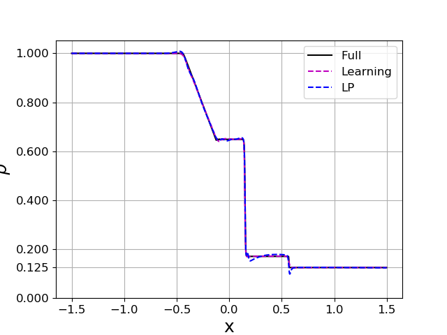
(a) 20 basis functions, density

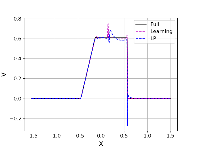
(b) 20 basis functions, velocity

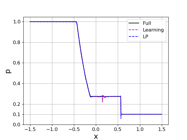
(c) 20 basis functions, pressure

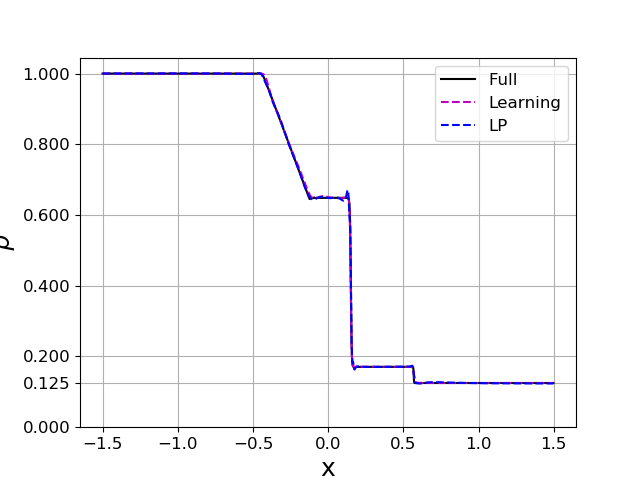
(d) 30 basis functions, density

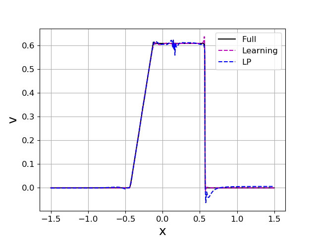
(e) 30 basis functions, velocity

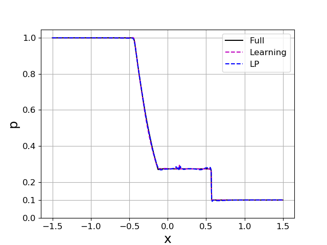
(f) 30 basis functions, pressure

Figure 4.24: Predicted solutions for the Euler equation in Section 4.8 at $t=0.25$.

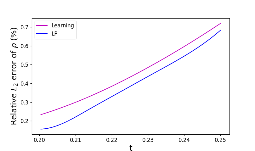
(a) 20 basis functions, density

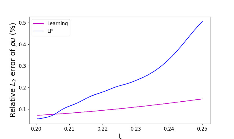
(b) 20 basis functions, velocity

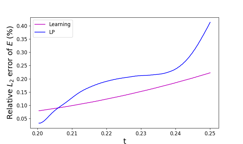
(c) 20 basis functions, pressure

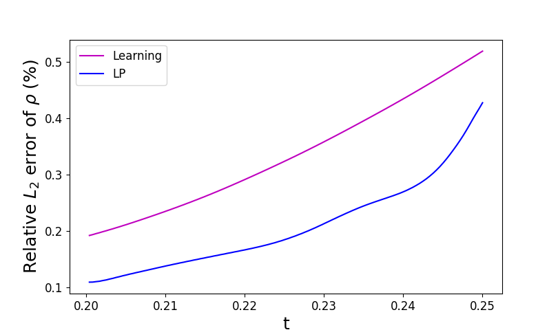
(d) 30 basis, density

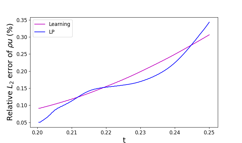
(e) 30 basis functions, velocity

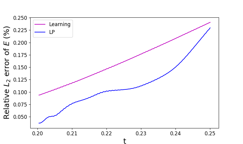
(f) 30 basis functions, pressure

Figure 4.25: The evolution of the prediction relative error of the Euler equation in Section 4.8 from $t=0.2$ to $t=0.25$.

5 Conclusions

Following the offline-online decomposition, we propose a learning-based projection method for transport problems.

As a combination of deep learning and the projection-based method, the proposed method has the following advantages:

1. Compared with the standard POD methods, it achieves smaller long-time prediction error with the same number of basis functions.

2. Compared with a pure learning-based method using the same neural network, the online projection step may reduce the generalization error dramatically.

3. Unlike previous learning-based projection methods [28, 29, 26], there is no need to take derivatives of neural networks in the online projection step.

4. With $x$ as an input of the neural network in a mesh free manner, it is flexible and simple for the proposed method to work with different meshes and even different schemes in the online and offline stages.

However, for problems with strong shocks, the projection based online stage may produce more numerical oscillation compared with a pure learning-based online stage.

There are still many aspects in this topic that could be further explored.

1. To design an efficient and robust hyper-reduction strategy to save the computational cost with explicit time integrators.

2. The effective and efficient control of numerical oscillations is crucial, especially when combined with hyper-reduction.

3. To apply and test the proposed method with more complicated 2D and 3D system hyperbolic conservation laws.

4. To further combine the proposed method with the adaptive moving mesh and the $h,p$-adaptive numerical methods which move or regenerate computational meshes for different time and/or parameter samples.

5. One drawback of the proposed method is that the learned basis is not orthonormal. To improve the robustness associated with this, one may introduce a regularization term similar to [59] in the loss function.

Appendix A More on the oscillation in Figure 4.12 with $r=15$

In Figure 4.12, non-physical oscillation can be observed in the reduced order solution generated by the LP method with $r=15$. To gain some understanding to the origin of such oscillation, in Figures 26(a)-26(f), we present the evolution of the full order solution, reduced order solution by the proposed LP method, and the $L^{2}$ projection of the full order solution onto the learned adaptive reduced space. At $t=0.6$, all three curves match well, with slight difference observed in the zoomed-in plot. At $t=0.7$, the oscillation in both the LP solution and the projection becomes quite visible. At $t=1.0$, the oscillation in the LP solution remains and spreads out, while the projection of the full order solution displays little difference from the full order solution. In Figures 26(g)-26(h), we further overlay the 15 learned basis functions and the full order solution at $t=0.7$ and $t=1.0$, respectively. One can see that the learned basis functions faithfully capture the local nature of the full order solution, without visible oscillation in themselves. The basis functions at these two different times also capture the propagation of the solution as well as its slight reduction in amplitude as time increases. From the observations above, we attribute the numerical oscillation in the LP solution with $r=15$ to the accumulation of the errors over time, the extrapolation of the basis functions from the training set to a test sample, and also to the online projection step. The underlying media is inhomogeneous, and this also contributes to the difference observed at $t=0.7$ and $t=1.0$ in the shape and amplitude of the basis functions and hence of the oscillation in the LP solution. Adaptively adding artificial viscosity in the online phase of the LP method to control these oscillations is worthy future research.

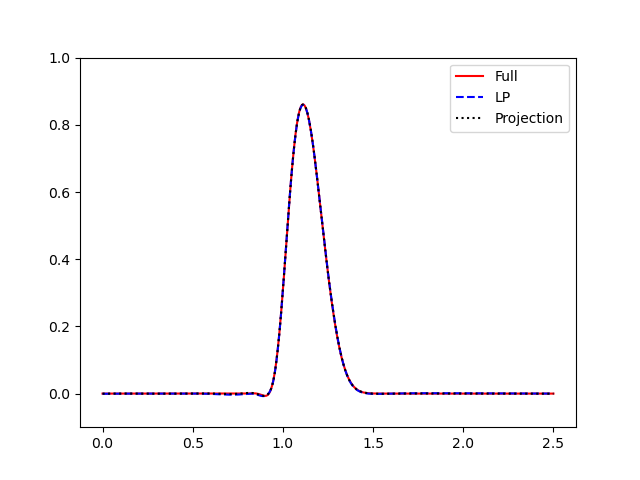
(a) $t=0.6$

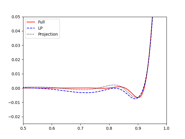
(b) $t=0.6$, zoomed-in

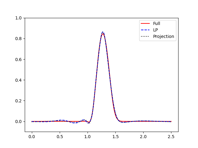
(c) $t=0.7$

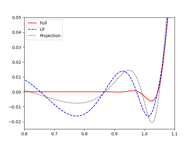
(d) $t=0.7$, zoomed-in

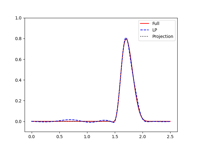
(e) $t=1.0$

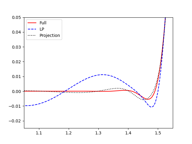
(f) $t=1.0$, zoomed-in

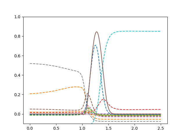
(g) $15$ basis functions (dashed lines) and the full order solution (solid line) at $t=0.7$

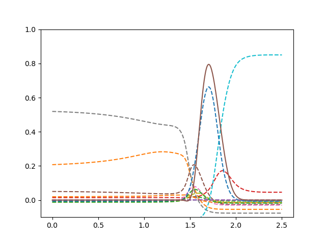
(h) $15$ basis functions (dashed lines) and the full order solution (solid line) at $t=1.0$

Figure A.26: The inhomogeneous media example in Section 4.5. (a)-(f): solutions at different times, where “Full” is the full order solution, “LP” is by the learning-based projection method, and “Projection” is the $L^{2}$ projection of the full order solution onto the learned reduced subspace. (g)-(h): $15$ learned basis functions (dashed lines) and the full order solution (solid line) at $t=0.7$ and $t=1.0$.

Acknowledgement. The authors want to thank Dr. Juntao Huang from Michigan State University for generously sharing his WENO codes solving the compressible Euler system.

References

- [1] Martín Abadi, Paul Barham, Jianmin Chen, Zhifeng Chen, Andy Davis, Jeffrey Dean, Matthieu Devin, Sanjay Ghemawat, Geoffrey Irving, Michael Isard, et al. Tensorflow: A system for large-scale machine learning. In 12th USENIX symposium on operating systems design and implementation (OSDI 16), pages 265–283, 2016.
- [2] Beatrice Battisti, Tobias Blickhan, Guillaume Enchery, Virginie Ehrlacher, Damiano Lombardi, and Olga Mula. Wasserstein model reduction approach for parametrized flow problems in porous media. 2022.
- [3] Peter Benner, Mario Ohlberger, Albert Cohen, and Karen Willcox. Model reduction and approximation: theory and algorithms. SIAM, 2017.
- [4] Gal Berkooz, Philip Holmes, and John L Lumley. The proper orthogonal decomposition in the analysis of turbulent flows. Annual review of fluid mechanics, 25(1):539–575, 1993.
- [5] W-J. Beyn and V. Thümmler. Freezing solutions of equivariant evolution equations. SIAM Journal on Applied Dynamical Systems, 3(2):85–116, 2004.
- [6] Annalisa Buffa, Yvon Maday, Anthony T Patera, Christophe Prud’homme, and Gabriel Turinici. A priori convergence of the greedy algorithm for the parametrized reduced basis method. ESAIM: Mathematical Modelling and Numerical Analysis-Modélisation Mathématique et Analyse Numérique, 46(3):595–603, 2012.
- [7] N. Cagniart. A few nonlinear approaches in model order reduction. PhD thesis, Sorbonne Université, 2018.
- [8] N. Cagniart, R. Crisovan, Y. Maday, and R. Abgrall. Model order reduction for hyperbolic problems: a new framework. 2017.
- [9] Nicolas Cagniart, Yvon Maday, and Benjamin Stamm. Model order reduction for problems with large convection effects. In Contributions to partial differential equations and applications, pages 131–150. Springer, 2019.
- [10] K. Carlberg. Adaptive -refinement for reduced-order models. International Journal for Numerical Methods in Engineering, 102(5):1192–1210, 2015.
- [11] Yanlai Chen, Sigal Gottlieb, Lijie Ji, and Yvon Maday. An EIM-degradation free reduced basis method via over collocation and residual hyper reduction-based error estimation. arXiv preprint arXiv:2101.05902, 2021.
- [12] Youngsoo Choi, Deshawn Coombs, and Robert Anderson. SNS: a solution-based nonlinear subspace method for time-dependent model order reduction. SIAM Journal on Scientific Computing, 42(2):A1116–A1146, 2020.
- [13] Albert Cohen, Ronald Devore, Guergana Petrova, and Przemyslaw Wojtaszczyk. Optimal stable nonlinear approximation. Foundations of Computational Mathematics, pages 1–42, 2021.
- [14] Wolfgang Dahmen, Min Wang, and Zhu Wang. Nonlinear Reduced DNN Models for State Estimation. arXiv preprint arXiv:2110.08951, 2021.
- [15] V. Ehrlacher, D. Lombardi, O. Mula, and F-X. Vialard. Nonlinear model reduction on metric spaces. Application to one-dimensional conservative PDEs in Wasserstein spaces. ESAIM: Mathematical Modelling and Numerical Analysis, 2019.
- [16] Andrea Ferrero, Tommaso Taddei, and Lei Zhang. Registration-based model reduction of parameterized two-dimensional conservation laws. arXiv preprint arXiv:2105.02024, 2021.
- [17] Stefania Fresca, Andrea Manzoni, et al. A comprehensive deep learning-based approach to reduced order modeling of nonlinear time-dependent parametrized PDEs. Journal of Scientific Computing, 87(2):1–36, 2021.
- [18] J-F. Gerbeau and D. Lombardi. Approximated Lax pairs for the reduced order integration of nonlinear evolution equations. Journal of Computational Physics, 265:246–269, 2014.
- [19] J-F. Gerbeau, D. Lombardi, and E. Schenone. Reduced order model in cardiac electrophysiology with approximated Lax pairs. Advances in Computational Mathematics, 41(5):1103–1130, 2015.
- [20] Carmen Gräßle and Michael Hinze. POD reduced-order modeling for evolution equations utilizing arbitrary finite element discretizations. Advances in Computational Mathematics, 44(6):1941–1978, 2018.
- [21] C. Greif and K. Urban. Decay of the Kolmogorov N-width for wave problems. Applied Mathematics Letters, 96:216–222, 2019.
- [22] Martin Gubisch and Stefan Volkwein. Proper orthogonal decomposition for linear-quadratic optimal control. Model reduction and approximation: theory and algorithms, 5:66, 2017.
- [23] Jiequn Han, Chao Ma, Zheng Ma, and E Weinan. Uniformly accurate machine learning-based hydrodynamic models for kinetic equations. Proceedings of the National Academy of Sciences, 116(44):21983–21991, 2019.
- [24] Jan S Hesthaven, Gianluigi Rozza, Benjamin Stamm, et al. Certified reduced basis methods for parametrized partial differential equations, volume 590. Springer, 2016.
- [25] Guang-Shan Jiang and Chi-Wang Shu. Efficient implementation of weighted eno schemes. Journal of computational physics, 126(1):202–228, 1996.
- [26] Y. Kim, Y. Choi, D. Widemann, and T. Zohdi. A fast and accurate physics-informed neural network reduced order model with shallow masked autoencoder. arXiv:2009.11990, 2020.
- [27] M. Kirby and D. Armbruster. Reconstructing phase space from PDE simulations. Zeitschrift für angewandte Mathematik und Physik ZAMP, 43(6):999–1022, 1992.
- [28] K. Lee and K. Carlberg. Deep Conservation: A latent dynamics model for exact satisfaction of physical conservation laws. arXiv:1909.09754, 2019.
- [29] K. Lee and K. Carlberg. Model reduction of dynamical systems on nonlinear manifolds using deep convolutional autoencoders. Journal of Computational Physics, 404:108973, 2020.
- [30] Kookjin Lee, Nathaniel A Trask, Ravi G Patel, Mamikon A Gulian, and Eric C Cyr. Partition of unity networks: deep hp-approximation. arXiv:2101.11256, 2021.
- [31] Hannah Lu and Daniel M Tartakovsky. Lagrangian dynamic mode decomposition for construction of reduced-order models of advection-dominated phenomena. Journal of Computational Physics, 407:109229, 2020.
- [32] Hannah Lu and Daniel M Tartakovsky. Dynamic Mode Decomposition for Construction of Reduced-Order Models of Hyperbolic Problems with Shocks. Journal of Machine Learning for Modeling and Computing, 2(1), 2021.
- [33] Lu Lu, Pengzhan Jin, and George Em Karniadakis. Deeponet: Learning nonlinear operators for identifying differential equations based on the universal approximation theorem of operators. arXiv:1910.03193, 2019.
- [34] Yvon Maday and Benjamin Stamm. Locally adaptive greedy approximations for anisotropic parameter reduced basis spaces. SIAM Journal on Scientific Computing, 35(6):A2417–A2441, 2013.
- [35] R. McCann. A convexity principle for interacting gases. Advances in mathematics, 128(1):153–179, 1997.
- [36] Jens M Melenk. On -widths for elliptic problems. Journal of mathematical analysis and applications, 247(1):272–289, 2000.
- [37] Rambod Mojgani and Maciej Balajewicz. Lagrangian basis method for dimensionality reduction of convection dominated nonlinear flows. arXiv:1701.04343, 2017.
- [38] Rambod Mojgani and Maciej Balajewicz. Physics-aware registration based auto-encoder for convection dominated PDEs. arXiv preprint arXiv:2006.15655, 2020.
- [39] N. Nair and M. Balajewicz. Transported snapshot model order reduction approach for parametric, steady-state fluid flows containing parameter-dependent shocks. International Journal for Numerical Methods in Engineering, 117(12):1234–1262, 2019.
- [40] M. Nonino, F. Ballarin, G. Rozza, and Y. Maday. Overcoming slowly decaying Kolmogorov -width by transport maps: application to model order reduction of fluid dynamics and fluid–structure interaction problems. arXiv:1911.06598, 2019.
- [41] M. Ohlberger and S. Rave. Nonlinear reduced basis approximation of parameterized evolution equations via the method of freezing. Comptes Rendus Mathematique, 351(23-24):901–906, 2013.
- [42] Mario Ohlberger and Stephan Rave. Reduced basis methods: success, limitations and future challenges. In Proceedings of ALGORITMY, pages 1–12, 2016.
- [43] B. Peherstorfer. Model reduction for transport-dominated problems via online adaptive bases and adaptive sampling. SIAM Journal on Scientific Computing, 42(5):A2803–A2836, 2020.
- [44] Allan Pinkus. N-widths in Approximation Theory, volume 7. Springer Science & Business Media, 2012.
- [45] Julius Reiss, Philipp Schulze, Jörn Sesterhenn, and Volker Mehrmann. The shifted proper orthogonal decomposition: A mode decomposition for multiple transport phenomena. SIAM Journal on Scientific Computing, 40(3):A1322–A1344, 2018.
- [46] D. Rim, S. Moe, and R. LeVeque. Transport reversal for model reduction of hyperbolic partial differential equations. SIAM/ASA Journal on Uncertainty Quantification, 6(1):118–150, 2018.
- [47] D. Rim, B. Peherstorfer, and K. Mandli. Manifold approximations via transported subspaces: model reduction for transport-dominated problems. arXiv:1912.13024, 2019.
- [48] D. Rim, L. Venturi, J. Bruna, and B. Peherstorfer. Depth separation for reduced deep networks in nonlinear model reduction: distilling shock waves in nonlinear hyperbolic problems. arXiv:2007.13977, 2020.
- [49] Francesco Romor, Giovanni Stabile, and Gianluigi Rozza. Non-linear manifold ROM with Convolutional Autoencoders and Reduced Over-Collocation method. arXiv preprint arXiv:2203.00360, 2022.
- [50] C. Rowley, I. Kevrekidis, J. Marsden, and K. Lust. Reduction and reconstruction for self-similar dynamical systems. Nonlinearity, 16(4):1257, 2003.
- [51] C. Rowley and J. Marsden. Reconstruction equations and the Karhunen–Loève expansion for systems with symmetry. Physica D: Nonlinear Phenomena, 142(1-2):1–19, 2000.
- [52] Joachim Schöberl. C++ 11 implementation of finite elements in ngsolve. Institute for Analysis and Scientific Computing, Vienna University of Technology, 30, 2014.
- [53] Chi-Wang Shu and Stanley Osher. Efficient implementation of essentially non-oscillatory shock-capturing schemes. Journal of computational physics, 77(2):439–471, 1988.
- [54] T. Taddei. A registration method for model order reduction: data compression and geometry reduction. SIAM Journal on Scientific Computing, 42(2):A997–A1027, 2020.
- [55] T. Taddei, S. Perotto, and A. Quarteroni. Reduced basis techniques for nonlinear conservation laws. ESAIM: Mathematical Modelling and Numerical Analysis, 49(3):787–814, 2015.
- [56] Huazhong Tang and Tao Tang. Adaptive mesh methods for one-and two-dimensional hyperbolic conservation laws. SIAM Journal on Numerical Analysis, 41(2):487–515, 2003.
- [57] Davide Torlo. Model reduction for advection dominated hyperbolic problems in an ALE framework: Offline and online phases. arXiv preprint arXiv:2003.13735, 2020.
- [58] C. Villani. Optimal transport: old and new, volume 338. Springer Science & Business Media, 2008.
- [59] Min Wang, Siu Wun Cheung, Wing Tat Leung, Eric T Chung, Yalchin Efendiev, and Mary Wheeler. Reduced-order deep learning for flow dynamics. The interplay between deep learning and model reduction. Journal of Computational Physics, 401:108939, 2020.
- [60] G. Welper. and -adaptive interpolation by transformed snapshots for parametric and stochastic hyperbolic PDEs. arXiv:1710.11481, 2017.
- [61] G. Welper. Interpolation of functions with parameter dependent jumps by transformed snapshots. SIAM Journal on Scientific Computing, 39(4):A1225–A1250, 2017.
- [62] G Welper. Transformed snapshot interpolation with high resolution transforms. SIAM Journal on Scientific Computing, 42(4):A2037–A2061, 2020.
- [63] Mary Fanett Wheeler. An elliptic collocation-finite element method with interior penalties. SIAM Journal on Numerical Analysis, 15(1):152–161, 1978.
- [64] Masayuki Yano. Discontinuous Galerkin reduced basis empirical quadrature procedure for model reduction of parametrized nonlinear conservation laws. Advances in Computational Mathematics, 45(5):2287–2320, 2019.
- [65] Masayuki Yano. Goal-oriented model reduction of parametrized nonlinear partial differential equations: Application to aerodynamics. International Journal for Numerical Methods in Engineering, 121(23):5200–5226, 2020.