Kolmogorov–Smirnov Test-Based Actively-Adaptive Thompson Sampling for Non-Stationary Bandits

Abstract

We consider the non-stationary multi-armed bandit (MAB) framework and propose a Kolmogorov-Smirnov (KS) test based Thompson Sampling (TS) algorithm named TS-KS, that actively detects change points and resets the TS parameters once a change is detected. In particular, for the two-armed bandit case, we derive bounds on the number of samples of the reward distribution to detect the change once it occurs. Consequently, we show that the proposed algorithm has sub-linear regret. Contrary to existing works, our algorithm is able to detect a change when the underlying reward distribution changes even though the mean reward remains the same. Finally, to test the efficacy of the proposed algorithm, we employ it in two case-studies: i) task-offloading scenario in wireless edge-computing, and ii) portfolio optimization. Our results show that the proposed TS-KS algorithm outperforms not only the static TS algorithm but also it performs better than other bandit algorithms designed for non-stationary environments. Moreover, the performance of TS-KS is at par with the state-of-the-art forecasting algorithms such as Facebook-PROPHET and ARIMA.

The applications of the multi-armed bandit (MAB) framework is well-established in literature. However, the non-stationary MAB problem is notoriously difficult to analyze mathematically. Contrary to the existing works, the proposed algorithm in this paper can detect a change in the environment when the underlying reward distribution changes even though the mean remains constant. In the task-offloading application in wireless edge-computing, and in the portfolio optimization problem, the proposed algorithm outperforms the contending algorithms across all time-windows. This work will find significant applications in epidemiology, e.g., in randomized clinical trials, wireless networks, computational advertisement, and financial portfolio design.

Multi-armed bandits, Thompson sampling, Kolmogorov-Smirnov test, edge-computing, 5G.

1 Introduction

In reinforcement-learning (RL), the multi-armed bandit (MAB) is a framework to facilitate sequential decision-making, wherein, a player selects a subset possible actions based on the rewards of previous action selections [2, 3, 4, 5]. The MAB framework has found applications in the fields of load demand sensing [6], online recommendation systems [7], computational advertisement [8], and wireless communications [9], among others. The MAB algorithms are particularly useful since they can directly be employed in an uncertain environment without any training phase. In the basic MAB setting, an agent (or player) chooses one out of $K$ independent choices (or arms), and obtains an associated reward. Each arm corresponds to a (possibly non-identical) reward distribution, that is unknown to the player. The objective of the player is to device an algorithm which minimizes the difference between the total rewards of the player and the highest expected reward, over a period of time, called the horizon $T$. To derive such an algorithm, the player maintains a belief associated to each choice as the temporal dynamics of the MAB setting evolves. Consequently, at each time-slot, the player selects the choice with the highest belief. This action-selection procedure presents an exploration-exploitation dilemma. In the classical setting, the reward distributions remain stationary over the entire time of play. However, most practical systems are characterized by a non-stationary reward framework, which is notoriously difficult to analyze analytically. Additionally, classical bandit algorithms are designed to select the arm with the highest mean reward. On the contrary, for several use-cases, such as portfolio optimization and clinical trials, an optimal arm may not be the one with the highest mean reward, but the one that achieves the best risk-reward balance. Recently, Zhu et al. [10] have developed modified TS algorithms for mean-variance bandits and provide comprehensive regret analyses for Gaussian and Bernoulli bandits. Indeed, for such use-cases, an algorithm that yields a lower expected payout but is less risky may be preferable. Since risk is characterized by the variance of the reward, a detection of the change in the cumulative density function (CDF) of the reward distribution becomes imperative. In this work, we propose and characterize a Kolmogorov-Smirnov (KS) test based bandit algorithm that provides asymptotic regret guarantees with an arbitrary probability.

Related Work: For stationary settings, several bandit algorithms, e.g., see [11] perform optimally. On the contrary, the Thompson Sampling (TS) algorithm [12], has gotten considerable interest recently due to its remarkably augmented performance vis-a-vis index-based policies [13]. However, the analytical characterization of the TS algorithm was challenging due to its randomized nature, until the work by Agarwal and Goyal [14].

In case of non-stationary reward distributions, most bandit algorithms loose mathematical tractability. For such non-stationary environments, researchers generally employ either of the two approaches: i) passively adaptive policies (e.g., see [15, 16]) which remain oblivious to the change instants and gradually decrease the weights given to past rewards, and ii) actively adaptive policies (e.g., see [17, 18, 19]) which track the changes and reset the algorithm on the detection of a change. Generally speaking, for the passively adaptive algorithms, rigorous performance bounds can be derived. Among the passively adaptive policies, Garivier and Moulines [15] have considered a scenario where the distribution of the rewards remain constant over epochs and change at unknown time instants. They have analyzed the theoretical upper and lower bounds of regret for the discounted upper confidence bound (UCB) (D-UCB) and sliding window UCB (SW-UCB). Besbes et al. [16] have developed a near optimal policy, REXP3. The authors have established lower bounds on the performance of any non-anticipating policy for a general class of non-stationary reward distributions. Following this, the optimal exploration exploitation trade-off for non-stationary environments were studied by the authors in [20].

On the other hand, actively adaptive algorithms outperform passively adaptive ones, as has been shown experimentally in e.g., [21]. Pertaining to the actively adaptive policies, Hartland et al. [17] have proposed an algorithm Adapt-EVE for abrupt changes in the environment. The change is detected via the Page-Hinkley statistical test (PHT). However, their evaluation is empirical and deviod of any performance bounds. PHT has found other applications, e.g., to adapt the window length of SW-UCL [22]. Furthermore, the works by Yu et. al [18] and Cao et al. [19] detect a change in the empirical means of the rewards of the arms. However, in both these works, the authors assume a fixed number of changes withing an interval to derive the respective bounds. The work that is closest to ours is [23], where the author assumed a change-detection based TS algorithm. However, similar to [18, 19], the author has proposed a change detection mechanism based on the comparison of means. On the same line, recently, Auer et al. [24] have proposed the algorithm ADSWITCH which is also based primarily on mean-estimation based checks for all the arms, and achieves nearly-optimal regret bounds without the prior knowledge of the total number of changes. Remarkably, the authors show regret guarantees for ADSWITCH without any pre-condition on the quanta of changes with each change point. However, such an algorithm fails to detect the change when the underlying distribution changes while the mean remains the same. Thus, there is a need to develop a MAB framework that is sensitive to change in the higher moments of the reward distribution. Such a setting can then be applied to the context of randomized clinical trial [25] in which the characteristic of the targeted pathogen changes abruptly (e.g., due to mutations), or, e.g., in computational advertisement in order to detect and adapt to a change in user profile [26]. On the contrary, in this work, we propose a detection mechanism based on the change of the CDFs. In particular:

• We introduce a novel change detection framework for the non-stationary MAB problem based on the KS goodness-of-fit test. The proposed algorithm detects a change when the underlying reward distribution changes even when the mean remains the same (e.g., [24, 19, 18]).

• Based on the KS test based change detection, we propose a actively adaptive TS algorithm called TS-KS, which resets the parameters of the classical TS algorithm on detection of the change. Furthermore, by considering a change in the mean of the Gaussian distributed rewards, we derive lower bounds on i) the number of samples of the reward distribution of an arm to accurately estimate its empirical cumulative distribution function (ECDF), and ii) the number of samples $n_{T}$ from the reward distribution. Consequently, we derive a bound on the regret of the TS-KS algorithm ans show that it has a sub-linear regret with an arbitrary probability. We also investigate the conditions under which the number of samples required by TS-KS is smaller than the state-of-the-art mean-estimation based change-detection methods.

• Finally, based on the TS-KS algorithm we present two case-studies. First, we investigate a task-offloading scenario in edge-computing where a secondary user in the network selects one out of a set of servers to offload a computational task in the presence of primary users. Then, we employ the proposed TS-KS algorithm in the portfolio optimization problem. Our result highlights that the proposed algorithm outperforms not only the classical TS algorithm, but also it perform better than other passively-adaptive and actively-adaptive TS algorithms that designed for non-stationary environments.

2 The Two-Armed Non-Stationary Bandit Setting

In this paper we study the two-armed bandit framework, with arms $a_{i}$, where $i\in\{1,2\}$. This framework is the same as the one considered in [23]. The player selects an arm at each time step $n$, and obtains a reward $R_{a_{i}}(n)$. The reward of arm $a_{i}$ is assumed to follow a Gaussian distribution, i.e., $R_{a_{i}}(n)\sim\mathcal{N}\left(\mu_{i}(n),\sigma^{2}\right)$, with non-stationary mean that is unknown to the player. Moreover, for the purpose of the mathematical analysis, we assume a fixed variance $\sigma^{2}$ across arms, although the framework is applicable in practice for the case when the variances are distinct across arms and piece-wise non-stationary. Additionally, let us consider the following lower bound on the difference between the mean reward of the two arms:

$$\left|\mu_{i}(n)-\mu_{j}(n)\right|\geq\Delta_{\mu},\quad{i\neq j},\forall n.$$ (1)

In our work, we consider a piecewise-sationary environment in which the values of $\mu_{i}(n)$ change at random time-instants, $T_{C_{l}}$, $l=1,2,\ldots$, with $T_{C_{0}}$ is at $n=0$. In particular, we assume that the change instants follow a Poisson arrival process with parameter $\lambda_{C}$. Thus, the quantity $T_{C_{l+1}}-T_{C_{l}}$ is exponentially distributed:

$$\mathbb{P}\left(T_{C_{l+1}}-T_{C_{l}}\leq k\right)=1-\exp\left(-\lambda_{C}k\right).$$ (2)

Thanks to the memoryless property of the exponential random variable, each arrival is stochastically independent to all the other arrivals in the process. Thus, in contrast to the existing studies that consider a fixed number of changes (e.g., see [18, 19, 24]), we consider a framework with a random number of changes governed by the intensity parameter $\lambda_{C}$. This reflects in the parameter $\lambda_{C}$ appearing in the regret bound of our algorithm as compared to e.g., the exact number of changes in [24]. The case with a fixed number of changes is thus a realization of the Poisson arrival process that occur with a Poisson probability distribution function. Furthermore, we assume that both the arms change simultaneously at $T_{C_{l}}$. Thus, in contrast to the existing studies that consider a fixed number of changes (e.g., see [18, 19, 24]), we study a framework consisting of a random number of changes governed by the intensity parameter $\lambda_{C}$. Owing to the independent scattering property of the Poisson arrival process, the presented framework models a completely random change-point arrival process. Furthermore, we assume that the mean rewards of the same arm across different time slots is bounded as:

$$\left|\mu_{i}(n)-\mu_{i}(k)\right|\in\{0\}\cup\left[\Delta_{\min},\Delta_{\max}\right],\quad n\neq k.$$ (3)

In particular, either the mean of the reward of an arm does not change, or it changes uniformly by a magnitude bounded between $\Delta_{\min}$ and $\Delta_{\max}$. Note that as discussed later in Proposition 1, the KS-test based change detection works even when $\Delta_{\min}=0$ as long as $\sigma_{2}\neq\sigma_{1}$. However, we consider a change in the reward distribution to be characterized by a change in the corresponding means so as to enable a fair comparison with the state-of-the-art mean-estimation based actively adaptive bandit algorithms.

At this point, it can be noted that the minimum difference in the mean reward before and after a change point, i.e., $\Delta_{\min}$ is equivalent to $2\epsilon$ in [18] and $\delta_{k}$ in [19].

Regret The function of an algorithm $\pi$ is to make a decision at each time step $n$, regarding $a_{\pi}(n)$, i.e., which arm to play. Consequently, $\pi$ receives a reward $R_{a_{\pi}}(n)\sim\mathcal{N}\left(\mu_{a_{\pi}}(n),\sigma^{2}\right)$. To characterize the regret performance of the algorithm, let at a time-step $n$, the optimal arm be denoted by $a_{i}$. Then, the regret after $T$ rounds of action-selection is given by:

$$\mathcal{R}(T)=\sum_{n=0}^{T}\left(\mu^{*}(n)-\mu_{a_{\pi}}(n)\right).$$

The aim is to devise a policy $\pi$ that achieves a bound on the expected regret: $\mathbb{E}\left[\mathcal{R}(T)\right]$. In this regard, in the next section we discuss the proposed KS-test based change-detection mechanism that tracks changes in the environment.

Algorithm 1 TS-KS

1:Parameters: $n_{T}$, $N$, $t_{ref}$, $T$.

2:Initialization: Count = 1, $\mathcal{S}_{j}=\{\}$ $\forall{j}\in\{1,2\}$ $\alpha_{j}=1,\beta_{j}=1$ $\forall{j}\in\{1,2\}$

3:for $t=1,2,\ldots,T$ do

4:     $\theta_{j}\sim Beta(\alpha_{j},\beta_{j})\forall j\in\{1,2\}$

5:     Play arm $a_{k}$ such that $k=\operatorname{argmax_{j}}\theta_{j}$

6:     Observe reward $\tilde{r_{t}}$

7:     $\mathcal{S}_{k}=\mathcal{S}_{k}\cup\tilde{\{r_{t}\}}$ $\triangleright$ Store reward

8:     $R_{\pi}(t)\leftarrow\dfrac{\tilde{r_{t}}-\mu_{\min}-\sigma Q^{-1}\left(\epsilon_{b}\right)}{2\sigma Q^{-1}\left(\epsilon_{b}\right)+\mu_{\max}-\mu_{\min}}$

9:     Obtain $x_{t}\sim{\rm Bernoulli}(\tilde{R_{\pi}(t)})$ $\triangleright$ Bernoulli Trial

10:     Update $\alpha_{k}=\alpha_{k}+x_{t}$ and $\beta_{k}=\beta_{k}+1-x_{t}$

11:     Count = Count + 1

12:     if Count $>(T_{N}+n_{T})$ then

13:         Identify optimal arm $k_{b}\doteq\operatorname{argmax_{j}}\frac{\alpha_{j}}{\alpha_{j}+\beta_{j}}$

14:         $\mathcal{S}_{t}=\cup_{i=L-n}^{L}\mathcal{S}_{k_{b}}(i)$ $\triangleright$ Test Sequence

15:         $\mathcal{S}_{e}=\cup_{i=L-n-N}^{L-n}\mathcal{S}_{k_{b}}(i)$ $\triangleright$ Estimate Sequence

16:         $t_{stat}$ = KS2Samp($S_{e}$, $S_{t}$) $\triangleright$ K-S Test

17:         if $t_{stat}>t_{ref}$ then

18:              Count = 1 $\triangleright$ Change Detected

19:              $\alpha_{j}=1,\beta_{j}=1$ $\forall{j}\in\{1,2\}$ $\triangleright$ Reset

20:         end if

21:     end if

22:end for

Algorithm 2 KS2Samp

1:Parameters: $n$, $N$, $\mathcal{S}_{t}$, $\mathcal{S}_{e}$.

2:$F_{\mathcal{S}_{t}}\leftarrow ECDF(\mathcal{S}_{t})$ $\triangleright$ Emperical CDF of test set

3:$F_{\mathcal{S}_{e}}\leftarrow ECDF(\mathcal{S}_{e})$ $\triangleright$ Emperical CDF of estimated set

4:$t_{stat}=\sqrt{\frac{nN}{n+N}}\operatorname{sup}_{z}|F_{\mathcal{S}_{t}}(z)-F_{\mathcal{S}_{e}}(z)|$

5:Return $t_{stat}$

3 KS Test based TS Framework

In this section, we describe the proposed TS algorithm which actively detects a change-point based on the KS test. First let us recall the classical TS algorithm. It assumes a Beta distribution, $\mathcal{B}(\alpha_{k},\beta_{k})$ to be the prior belief for the distribution of the rewards of each arm. The parameters $\alpha_{k},\beta_{k}$ are initialized to 1. Then, at each $n$, the player generates an instance $\theta_{k}\sim\mathcal{B}(\alpha_{k},\beta_{k}),\forall k\in\{1,2\}$. Consequently, it plays the choice $k=\operatorname*{arg\,max}_{j}\theta_{j}$ and obtains a reward $R(n)$. Due to the assumption of normal distributed rewards, the values that the reward can take is in the range $R(n)\in(-\infty,\infty)$. However, for the sake of tractability and to employ the TS algorithm of [14], we map $R(n)$ to the range $[0,1]$ [23]. For each arm, let us define $L$ and $U$ as: $\mathcal{P}(L\leq R_{a_{j}(n)}\leq U)\geq 1-2\epsilon_{b},\quad\forall j\in\{1,2\},$ where, $\epsilon_{b}$ is an arbitrary small positive number. Naturally, the values of $U$ and $L$ depend on the maximum and minimum values of $\mu_{j}$, respectively. Accordingly, let us define:

$$\mu_{\max} =\max{\mu_{j}(n)},\quad\forall j,n\quad\mbox{and,}$$

$$\mu_{\min} =\min{\mu_{j}(n)},\quad\forall j,n$$

as the bounds of the mean rewards. Consequently, $U$ and $L$ can be calculated as: $U=\sigma Q^{-1}\left(\epsilon_{b}\right)+\mu_{\max}$ and $L=\mu_{\min}-\sigma Q^{-1}\left(\epsilon_{b}\right),$ where $Q^{-1}(\cdot)$ is the inverse of the Gaussian $Q$-function. Accordingly, we define $R_{\pi}(n)=\frac{R_{a_{j}}(n)-L}{U-L}$, which ensures that $0\leq R_{\pi}(n)\leq 1$ with a probability $1-2\epsilon_{b}$. and perform a Bernoulli trial with a success probability $R_{\pi}$ [14] with an outcome $x(n)$. Of course, for the reward distributions that are naturally restricted within a finite domain (e.g., Bernoulli rewards), this step is not necessary and the rest of the algorithm follows without this step.

The posterior distribution is consequently updated as $\alpha_{k}=\alpha_{k}+x(n)$ and $\beta_{k}=\beta_{k}+1-x(n)$. The sequence of the obtained rewards by the agent for each arm $j$ is used to generate a reward set $\mathcal{S}_{j}$. In our work, the distribution of the rewards are stationary for $T_{F}\geq T_{N}+n_{T}$ after each change. After $T_{N}$ plays of the bandit algorithm, the change-detection mechanism initiates. Each $\mathcal{S}_{j}$ is updated after every play for $a_{j}$ (i.e., the optimal arm), until the change is detected. In case the environment remains stationary, the beliefs of both the arms provide an accurate estimate of their respective CDFs. On the contrary, when the reward distributions of the both the arms change over time, the player has to adapt when such a change is detected. This is described in the what follows.

Active Change-point Detection: To actively detect the change-points, the proposed algorithm uses the two sample KS test [27]. In particular, the algorithm stores the rewards of the arm $a_{k}$ in a sequence $\mathcal{S}_{k}$ which is updated each time the arm $a_{k}$ is played. From the sequence $\mathcal{S}_{k}(\cdot)$, we create two sub-sequences: i) the test sequence $\mathcal{S}_{t}(\cdot)$: the rewards for the last $n_{T}$ plays of arm $j$, and ii) the estimate sequence $\mathcal{S}_{e}(\cdot)$: the rewards for the last $N$ rewards before the previous $n_{T}$ plays. In other words, if the cardinality of $\mathcal{S}_{j}$ is $L$, we have $\mathcal{S}_{t}=\cup_{i=L-n_{T}}^{L}\mathcal{S}_{k_{b}}(i)$ and $\mathcal{S}_{e}=\cup_{i=L-n_{T}-N}^{L-n_{T}}\mathcal{S}_{k_{b}}(i)$. Consequently, TS-KS constructs the ECDF of $\mathcal{S}_{t}$ and $\mathcal{S}_{e}$, denoted by $F_{\mathcal{S}_{t}}(\cdot)$ and $F_{\mathcal{S}_{e}}(\cdot)$, respectively.

Next, we calculate the Kolmogorov distance between the two ECDFs as $D_{n_{T},N}=\operatorname{sup}_{z}|F_{\mathcal{S}_{t}}(z)-F_{\mathcal{S}_{e}}(z)|$ and compare it with a reference test statistic value $t_{ref}$. In case $D_{n_{T},N}>t_{ref}$, the test concludes that the two set of samples belong to two different probability distributions, and a change is detected. On the contrary, if $D_{n,m}<t_{ref}$, the two set of samples are considered to be i.i.d. from the same distribution.

The parameter $N$ is the minimum number of samples needed to form an accurate ECDF of the reward distribution before the change point. On the other hand, the parameter $n_{T}$ is the minimum number of samples after the change-point needed to correctly detect a change. In the next section, we derive the theoretical bounds on the parameters $n_{T}$ and $N$.

4 Theoretical Bounds

Let the reward distribution of the optimal arm before the change-point $T_{C_{l}}$ be denoted by $\rho_{l}\sim\mathcal{N}(\mu_{l},\sigma^{2})$ and after the change-point be denoted by $\rho_{l+1}\sim\mathcal{N}(\mu_{l+1},\sigma^{2})$. Without loss of generality, it is assumed that $\mu_{l+1}>\mu_{l}$. Let us denote the CDF of $\rho_{l}$ by $F_{l}(x)$ and CDF of $\rho_{l+1}$ by $F_{l+1}(x)$. Let us mathematically characterize the accuracy of the ECDF $F_{\mathcal{S}_{e}}$ from $N$ observed samples. Note that contrary to [23], for the TS-KS algorithm, merely an estimate of the mean of the arm is not sufficient, and the framework must estimate the CDF of the reward distribution. For this, let us first introduce the following definition:

Definition 1.

An ECDF $\hat{F}_{X}(x)$ of a random variable $X$ formed from $K$ samples is defined to be accurate with respect to its actual CDF $F_{X}(x)$ if:

$$D_{K}=\operatorname{sup}_{x}|\hat{F}_{X}(x)-F_{X}(x)|\leq t_{ref}.$$

The above definition follows from the one-sample KS test of $\hat{F}_{X}(x)$ with respect to $F_{X}(x)$. Thus, for the ECDF of $\mathcal{S}_{e}$ to be accurate, the following condition must be satisfied:

$$D_{N}=\operatorname{sup}_{x}|F_{\mathcal{S}_{t}}-F_{l}(x)|\leq t_{ref}.$$ (4)

Proposition 1.

The KS-test detects a change in the bandit framework when the reward distributions change even when the mean of the rewards remain constant.

The KS statistic, defined by the supremum of the absolute value of the difference of the CDFs. Let $F_{S_{t}}\sim\mathcal{N}(\mu_{l},\sigma_{l}^{2})$ and $F_{l}\sim\mathcal{N}(\mu_{l+1},\sigma_{l+1}^{2})$, for a generic values of $\mu_{l},\mu_{l+1},\sigma_{l}$ and $\sigma_{l+1}$. Then, the supremum of $|F_{S_{t}}(x)-F_{l}(x)|$ is

$$D= \frac{1}{2}\left(\operatorname{erf}\left(\frac{\sigma_{l}^{2}(\mu_{l+1}-\mu_{l})-y_{1}}{\sqrt{2}\sigma_{l}(\sigma_{l}^{2}-\sigma_{l+1}^{2})}\right)-\right.$$

$$\left.\operatorname{erf}\left(\frac{\sigma_{l+1}^{2}(\mu_{l+1}-\mu_{l})-y_{1}}{\sqrt{2}\sigma_{l+1}(\sigma_{l}^{2}-\sigma_{l+1}^{2})}\right)\right)$$ (5)

where,

$$y_{1}= \sigma_{l}\sigma_{l+1}\left(2\sigma_{l}^{2}\log\left(\frac{\sigma_{l}}{\sigma_{l+1}}\right)-2\mu_{l}\mu_{l+1}-\right.$$

$$\left.2\sigma_{l+1}^{2}\log\left(\frac{\sigma_{l}}{\sigma_{l+1}}\right)+\mu_{l}^{2}+\mu_{l+1}^{2}\right)^{\frac{1}{2}}.$$ (6)

Accordingly, for $\sigma_{1}\neq\sigma_{2}$, the value of $D$ is non-zero even if $\mu_{l}=\mu_{l+1}$. Accordingly, for fixed mean, and a suitable threshold, the KS-test is able to detect a change in the environment which the mean-estimation based detection misses.

However, in what follows, we focus on the case when $\sigma_{1}=\sigma_{2}=\sigma$ and $\mu_{l}\neq\mu_{l+1}$. In the following Lemma, we bound the number of elements $N$ of $\mathcal{S}_{e}$ for the ECDF of the optimal arm to be accurate with respect to its actual CDF with a probability of at least $1-p_{loc}$.

Lemma 1.

The number of samples $N$ for which the ECDF of the optimal arm is accurate with respect to its $F_{l}(x)$ with probability greater than $1-p_{loc}$ is:

$$N\geq\frac{1}{2t_{ref}^{2}}\ln\left(\frac{2}{p_{loc}}\right)$$

We recall the Dvoretzky–Kiefer–Wolfowitz-Massart (DKWM) inequality [28] to bound the probability that the Kolmogorov distance of the ECDF with $N$ samples to its actual CDF is greater than $t_{ref}$ as:

$$\mathbb{P}\left(\sup_{x\in\mathbb{R}}|{F}_{\mathcal{S}_{t}}(x)-F_{l}(x)|>t_{ref}\right)\leq 2\exp\left(-2Nt_{ref}^{2}\right),$$

$$\qquad\forall t_{ref}>0.$$ (7)

Accordingly, we bound the right hand side as $2\exp\left(-2Nt^{2}_{ref}\right)\leq p_{loc}$ to complete the proof. Next, we evaluate the number of plays of the stationary bandit framework so that at least $N$ plays of the optimal arm occurs. First, let us note that in order to have at least one of the arms played at least $N$ times, the total number of plays is lower bounded by $T_{N}=2N$. On the other hand, for several applications where the variance of performance of the classical TS algorithm remains constant, we have the following result.

Lemma 2.

For the special case when the variance of the TS algorithm is low so that the approximation $N\approx\mathbb{E}[N]$ holds true, the number of plays so that the optimal arm is played at least $N$ times is given by:

$$T\geq T_{N}=\frac{160}{\Delta^{2}_{\mu}}\log\left(\frac{80}{\Delta^{2}_{\mu}}\right)+2\left[\frac{48}{\Delta^{4}_{\mu}}+18+N\right].$$

For this result, first let us consider the number of plays of the TS algorithm in the stationary regime, such that the optimal arm is played $N$ times. This in turn characterizes an accurate estimate of its CDF.

In the classical setting, if the TS algorithm is employed for $T$ plays, the mean plays of the sub-optimal $a_{j}$ is bounded as [14]: $\mathbb{E}\left[N_{j}\right]\leq\frac{40\ln T}{\Delta_{\mu}^{2}}+\frac{48}{\Delta_{\mu}^{4}}+18.$ Consequently, we want the number of plays of the optimal arm to satisfy the following criterion:

$$T-\left(\frac{40\ln T}{\Delta_{\mu}^{2}}+\frac{48}{\Delta_{\mu}^{4}}+18\right)\geq N,$$

$$\implies T\geq\frac{40\ln T}{\Delta^{2}_{\mu}}+\left[\frac{48}{\Delta^{4}_{\mu}}+18+N\right]$$ (8)

Then the statement of the lemma follows from applying Lemma A2 of [29].

Given the ECDF of the reward $\rho_{l}$ is accurate, we characterize the performance of the change-point detection. In particular, let the parameter $n_{T}$ denote the minimum number of plays required to detect a change. We recall that a change is detected with $n_{T}$ plays when the following condition holds true:

Lemma 3.

The maximum difference between the two CDFs of $\rho_{l}$ and $\rho_{l+1}$ is given by $\operatorname{sup}_{x}|F_{l}(x)-F_{l+1}(x)|=\operatorname{erf}(\frac{\mu_{l}-\mu_{l+1}}{2\sqrt{2}\sigma})$ and the point of maximum is $x_{\max}=\frac{\mu_{l}+\mu_{l+1}}{2}$

We assume the CDF before change-point follows the distribution $F_{l}\sim\mathcal{N}(\mu_{l},\sigma^{2})$ and CDF after the change-point follows the distribution $F_{l+1}\sim\mathcal{N}(\mu_{l+1},\sigma^{2})$. Therefore, the difference between the CDFs is given by the following equation:

$$|F_{l}(x)-F_{l+1}(x)|= \frac{1}{2}\left[1+\operatorname{erf}\left(\frac{x-\mu_{l}}{\sigma\sqrt{2}}\right)\right]-$$

$$\frac{1}{2}\left[1+\operatorname{erf}\left(\frac{x-\mu_{l+1}}{\sigma\sqrt{2}}\right)\right]$$

$$= \frac{1}{2}\left[\operatorname{erf}\left(\frac{x-\mu_{l}}{\sigma\sqrt{2}}\right)-\operatorname{erf}\left(\frac{x-\mu_{l+1}}{\sigma\sqrt{2}}\right)\right]$$ (9)

Next to find $D_{n}=\operatorname{sup}_{x}|F_{l}(x)-F_{l+1}(x)|$, we first differentiate the above function with respect to $x$ in order to obtain the maximum point:

$$\frac{\partial D_{n}}{\partial x}=\frac{1}{\sigma\sqrt{2\pi}}\left[e^{-\frac{1}{2}\left(\frac{x-\mu_{l}}{\sigma}\right)^{2}}-e^{-\frac{1}{2}\left(\frac{x-\mu_{l+1}}{\sigma}\right)^{2}}\right]=0$$

$$\implies e^{-\frac{1}{2}\left(\frac{x-\mu_{l}}{\sigma}\right)^{2}}-e^{-\frac{1}{2}\left(\frac{x-\mu_{l+1}}{\sigma}\right)^{2}}=0$$

Solving for $x$, we get:

$$x_{max}=\frac{\mu_{l}+\mu_{l+1}}{2}$$

Substituting the value of $x_{max}$ in $D_{n}$, we obtain:

$$\operatorname{sup}_{x}|F_{l}(x)-F_{l+1}(x)|=\operatorname{erf}\bigg{(}\frac{\mu_{l}-\mu_{l+1}}{2\sqrt{2}\sigma}\bigg{)}$$

Based on Lemma 3, we derive the lower bound on $n_{T}$ given by the following result.

Lemma 4.

Given the estimate of the ECDF $F_{\mathcal{S}_{e}}$ and $F_{\mathcal{S}_{t}}$ are accurate, for a false-alarm probability of $\mathcal{P}_{F}$, the minimum number of samples of $\rho_{l+1}$ required to limit the probability of missed detection to $\mathcal{P}_{M}$ is lower bounded as:

$$n\geq n_{T}=\frac{\ln\frac{2}{\mathcal{P}_{F}}}{2\operatorname{erf}^{2}\left(\frac{1}{2\sqrt{2}\sigma}\left(\mathcal{P}_{M}\left(\Delta_{\max}-\Delta_{\min}\right)+\Delta_{\min}\right)\right)}$$ (10)

The algorithm results in a false-alarm if it detects a change even if the test set and the estimate set are both sampled from the same reward distribution with CDF $F_{l}(x)$. By the DKWM inequality [28], for $t_{ref}>0$, we have:

$$\mathbb{P}\left({\mbox{False Alarm}}\right) =\mathbb{P}\left(\sup_{x}|F_{\mathcal{S}_{t}}(x)-F_{l}(x)|>t_{ref}\big{|}\mathcal{S}_{t}\sim\rho_{l}\right)$$

$$\leq 2\exp\left(-2nt_{ref}^{2}\right)$$ (11)

Equating this to $\mathcal{P}_{F}$, we get:

$$t_{ref}=\sqrt{\frac{1}{2n}\ln\frac{2}{\mathcal{P}_{F}}}$$ (12)

Recall that a missed detection occurs when the algorithm fails to detect a change, given that the test set and the estimate set are both sampled from two different reward distributions. From the condition of failure of change-point detection:

$$\mathbb{P}\left(\mbox{Missed Detection}\right)$$ (13)

$$=\mathbb{P}\left(\sup_{x}|F_{\mathcal{S}_{t}}(x)-F_{l}(x)|<t_{ref}|\mathcal{S}_{t}\sim\rho_{l+1}\right)$$

$$=\mathbb{P}\left(\operatorname{erf}\left(\frac{\Delta}{2\sqrt{2}\sigma}\right)<t_{ref}\right)$$

$$=\frac{2\sqrt{2}\sigma\operatorname{erf}^{-1}\left(t_{ref}\right)-\Delta_{min}}{\Delta_{\max}-\Delta_{\min}}$$

The last step follows from the uniform distribution of $\Delta$. Then, the result follows from the condition that $\mathbb{P}\left(\mbox{Missed Detection}\right)\leq\mathcal{P}_{M}$.

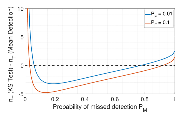
Figure 1: Comparison of the change-detection delay of TS-CD and TS-KS.

In Fig. 1, we compare the performance of the mean-estimation based change detection method [23] with the KS-test based change detection method for the special case when the reward distribution is associated with a change in the mean reward of the arms. We plot the difference in the number of samples required to detect a change between the two methods. In particular, we assume the distribution of the reward to be $\sim\mathcal{N}(\mu,\sigma)$ before the change point and $\leavevmode\nobreak\ \mathcal{N}(\mu+\Delta_{min},\sigma)$ after the change point. Then, the plot in the Figure 1 represents the difference in the number of samples after the change point that the two algorithms TS-KS and TS-CD take to detect the change. Thus, a negative value indicates that TS-KS is able to detect the change point with a fewer samples as compared to TS-CD.. For very low values of $\mathcal{P}_{M}$ (e.g., $<0.05$), the mean estimation based method detects a change with fewer samples as compared to the KS-test. This is because for such low values of $\mathcal{P}_{M}$, the KS-test requires a very high number of samples in order to create an accurate estimate of the CDF. On the other hand, for a large range of moderately tolerable missed detection probabilities (e.g., 0.1 to 0.7), the number of samples required by the KS-test is fewer than the mean based detection. It is thus important to note that the proposed KS-test must be employed on top of the bandit framework based on the type of application/service and its requirements characterized by a given missed detection probability. For stringent missed-detection constraints, the mean-estimation based change-detection should be employed since outperforms the KS-test.

Next, we study the bounds on the change arrival frequency so as to enable the TS-KS algorithm to track the changes in the environment.

Lemma 5.

To limit the probability of the frequency of change to $p_{change}$, the bound on the value of $\lambda_{A}$ is:

$$\lambda_{A}\leq\frac{1}{n_{T}+T_{N}}\ln\left(\frac{1}{1-p_{change}}\right).$$ (14)

This follows from (2). Finally, in what follows, we derive the bound on the regret of the TS-KS for given values of $\mathcal{P}_{M}$, $p_{loc}$, and $p_{change}$. For that, we first recall the result of [14] which states that for the stationary regime, the regret the TS algorithm is bounded by the order of $\mathcal{O}(\ln(T))$. Based on this, we derive the following result.

Theorem 1.

For the two-armed non-stationary bandit problem, with a probability

$$p_{tot}=\left(1-p_{loc}\right)\left(1-p_{change}\right)\left(1-\mathcal{P}_{M}\right),$$ (15)

the TS-KS algorithm has expected regret bound:

$$\mathbb{E}\left[\mathcal{R}(T)\right]\leq\mathcal{O}\left(\ln\left(T_{N}\right)\lambda_{A}T\left[\frac{\Gamma\left(\frac{T}{T_{N}+n_{T}},\lambda_{A}T\right)}{\Gamma\left(\frac{T}{T_{N}+n_{T}}\right)}\right]\right),$$ (16)

in time $T$, where $\Gamma(\cdot)$ is the Gamma function, and $\Gamma_{\mathrm{i}}(\cdot,\cdot)$ is the upper incomplete Gamma function. Thus, the time expected regret is asymptotically bounded, i.e., $\lim_{T\to\infty}\frac{1}{T}\mathbb{E}\left[\mathcal{R}(T)\right]=0.$

The proof follows similar to that in [23].

Table 1: Reference for Notations used

Symbol	Definition
$T$	Total number of time-steps/ Time horizon
$\tilde{r_{t}}\in\mathbb{R}$	Reward observed
$x_{t}\in\{0,1\}$	Outcome of the Bernoulli trail
$T_{C_{l}}$	Time-step of $l^{th}$ change-point
$F_{l}(x),F_{l+1}(x)$	CDF before/after change-point
$F_{n}(x)$	Empirical CDF formed from n samples
$D_{n}$	Test statistic value obtained from K-S test
$\mathcal{S}_{k}$	Reward cache for $k^{th}$ arm
$t_{ref}$	Reference test statistic value
$T_{N}$	No. of plays of the stationary MAB problem for $N$ plays of the optimal arm
$n_{T}$	No. of samples to detect a change
$\mathcal{P}_{F},\mathcal{P}_{M}$	Upper limit of the probability of false alarm and the probability missed detection

In order to investigate practical applications of our proposed method, in the next sections we perform two case-studies: edge-computing and algorithmic trading.

5 Case Study 1: Task Offloading in Edge-Computing

We consider an edge computing framework consisting of multiple edge servers denoted by the set $\mathcal{S}$ and multiple primary users denoted by the set $\mathcal{V}$. Each primary user connects to a server to offload a computing task. Additionally, we consider secondary users which opportunistically associate to a server for offloading their tasks based on the availability of the servers. The primary user-server association changes with time, thereby altering the short-term characteristics of the servers in terms of the amount of task pending to be processed, which we refer to as the workload buffer [30]. We model the task offloading process of a secondary-user in this network as the MAB problem. A secondary user makes a computation request to a server, that must perform the computation within the personal deadline of the secondary user, for the transaction to be counted as a successful service.

An epoch is defined as the duration for which the number of primary users associated to a server remains constant. Thus, the time axis is divided into sets of epochs, which we denote by $\mathcal{T}_{l}\equiv\left[T_{C_{l}},T_{C_{l+1}}\right)\cap\mathbb{N}$, where $l\in\mathbb{N}$ and $T_{C_{l}}$ denotes the $l^{\rm th}$ change-point. For an epoch $\mathcal{T}_{l}$, the size of the workload buffer at the beginning of this epoch, for server $s_{k}\in\mathcal{S}$ is $B_{0,l}^{k}$. Furthermore, the servers have a memory limit and accommodate a maximum workload buffer of size $B_{\max}^{k}$. The number of users associated with server $s_{k}\in\mathcal{S}$ in epoch $\mathcal{T}_{l}$ is $m_{l}^{k}$, and each primary user offloads task at the same rate of $\eta$ cycles/second. Finally, we assume that the server $s_{k}$ processes the workload at the rate of $C_{k}$ cycles/second.

The size of the workload buffer is modeled as:

$$B_{l}^{k}(t)=B_{0,l}^{k}+(m_{l}^{k}\cdot\eta-C_{k})\,(t-T_{C_{l}});\quad t\in\mathcal{T}_{l}.$$ (17)

Accordingly, conditioned on $m_{l}^{k}$, we model the value of $B_{l}^{k}(t),\forall t\in T_{C_{i}}$, from one of the following distributions:

$$B_{l}^{k}(t)\sim\begin{cases}\mathcal{U}\left(B_{0}^{l,k}+(m_{l}^{k}\cdot\eta-C_{k})\,|\mathcal{T}_{l}|,\quad B_{0}^{l,k}\right),&m_{l}^{k}\eta\leq C_{k}\\ \mathcal{U}\left(B_{0}^{l,k},\quad B_{0}^{l,k}+(m_{l}^{k}\cdot\eta-C_{k})\,|\mathcal{T}_{l}|\right),&m_{i}^{k}\eta>C_{k}\end{cases}$$

where $|\mathcal{T}_{l}|\triangleq T_{C_{l+1}}-T_{C_{l}}$.

5.1 User-Server association model

Next, we describe the primary user-server association model. Let us assume that a user $v_{j}\in\mathcal{V}$ changes its server association at intervals defined by an exponential process with parameter $\lambda_{j}$ (this model is used in e.g., [31]). Then, the interval for which the association of all the primary users remains unchanged is given by the epoch:

$$|\mathcal{T}_{l}|\sim\lambda_{C}\cdot\exp\left(-\lambda_{C}x\right);\quad\lambda_{C}\triangleq\sum_{j=1}^{|\mathcal{V}|}\lambda_{j},\quad x\in\mathbb{N}.$$ (18)

Since the users do not change their server associations within an epoch, we count the number of users associated $m_{l}^{k}\geq 0$ with any server $s_{k}$ by partitioning $\mathcal{V}$ users into $|\mathcal{S}|$ number of disjoint sets, i.e., $\sum_{s_{k}\in\mathcal{S}}m_{l}^{k}=|\mathcal{V}|,\forall l\in\mathbb{N}$.

$$\mathbf{m}_{l}\triangleq\Big{[}m_{l}^{1},m_{l}^{2},\cdots m^{|\mathcal{S}|}_{l}\Big{]}\sim\texttt{Partition}(\mathcal{V},|\mathcal{S}|).$$ (19)

Where, the Partition mechanism is be modelled as a multinomial distribution:

$$p_{\mathbf{m}_{l}}(\mathbf{m}_{l}=\mathbf{q}_{l})=\frac{|\mathcal{V}|!}{\prod_{k=1}^{|\mathcal{S}|}q_{l}^{k}!}|\mathcal{S}|^{-|\mathcal{V}|},$$ (20)

where each primary user is equally likely to connect to a server, i.e., probability of associating with a server $s_{k}$ is $\frac{1}{|\mathcal{S}|}$, which is independent of the server $s_{k}$.

5.2 Task Offload Mechanism and Reward Characterization

A secondary user wants to offload a task which takes $\delta$ cycles to process. Based on the workload buffer, the time required by server $s_{k}$ to generate the output is calculated as:

$$\zeta_{l}^{k}(t)=\frac{B_{l}^{k}(t)+\delta}{C_{k}}$$ (21)

For the a task offloading success, the output must be generated within the personal deadline $T_{\max}$ of the secondary user. Thus, the reward for TS is described as:

$$R_{s_{k}}(t)=\mathrm{1}\left\{\zeta_{l}^{k}(t)\leq T_{\max}\right\},\quad\forall t\in\mathcal{T}_{l}$$ (22)

For consistency with TS-KS, we map the reward in the continuous domain. Accordingly, we input the value $T_{\max}-\zeta_{l}^{k}(t)$ for Algorithm 2. This is intuitive, since negative values indicate that the deadline is exceeded and a positive value refers to the task being completed within the deadline.

Table 2: Simulation parameters

Parameter	Value	Unit
$B_{\max}^{k}$	$\sim\mathcal{U}(0.5,1)$	Giga-cycles
$C_{k}$	$\sim\mathcal{U}(2,4)$	GHz
$\eta$	8	Mbps
$\delta$	20	Mega-cycles
$1/\lambda_{C}$	$[50,500]$	s
$T_{\max}$	0.05	s

5.3 Results and Discussion

In Fig. 2, we show the evolution of the cumulative regret with time, for the various bandit algorithms. It is evident that TS-KS beats all other algorithms, as it has the lowest cumulative regret value. The performance of the change-point refresh based algorithms, namely TS-CD and TS-KS is comparable and both have similar variance. In contrast TS not only has the highest regret, but also the highest variance, which makes it the least reliable algorithm for non-stationary environments.

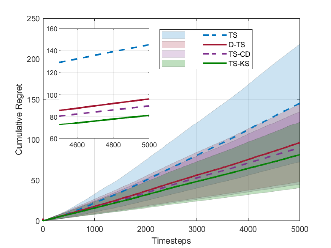
Figure 2: Cumulative Regret. $|\mathcal{S}|=3,|\mathcal{V}|=10^{3}$.

Next, in Fig. 3 we plot the values of mean normalized regret, for different values of mean epoch durations ($\frac{1}{\lambda_{C}}$) across the bandit algorithms under consideration. The value of mean epoch duration directly translates to the randomness of the environment; If the mean epoch duration is less, the reward distribution of the arms changes quickly and vice versa.

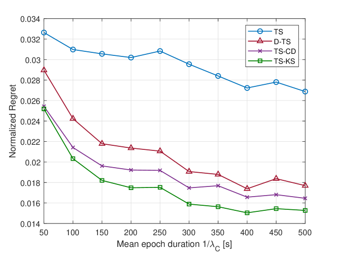
Figure 3: Regret variation against mean epoch duration. $|\mathcal{S}|=3,|\mathcal{V}|=10^{3},\frac{1}{\lambda_{C}}=300\leavevmode\nobreak\ s$.

We see that TS-KS maintains the lowest value of normalized regret across all values of mean epoch duration. As a common trend for all the algorithms, the mean normalized regret decreases as the environment becomes less random, i.e., the mean epoch duration increases.

6 Case Study 2: Portfolio Optimization

In the second case-study, we consider the problem of portfolio optimization [32]. A portfolio is defined as a collection of stocks which are selected on the basis of their associated risks and returns. We employ our TS-KS framework on the New York Stock Exchange dataset [33] and compare it with the contending algorithms. The dataset contains daily prices of 501 stocks spanning from 2010 to the end of 2016. The portfolios considered are $p_{1}$ = {Eaton Corporation, Whole Foods Market}, $p_{2}$ = {Union Pacific Corporation, IDEXX Laboratories}, $p_{3}$ = {Union Pacific Corporation} and $p_{4}$ = {Church & Dwights}. Then, we model each of the portfolios from the set $\mathcal{P}\equiv\{p_{1},p_{2},p_{3},p_{4}\}$ as an arm of the MAB setting. For this case-study, we focus only on buying stocks, and accordingly, all the reward returns are functions of unrealized profits in the stocks.

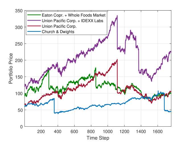
Figure 4: Portfolio price vs Time-step

In Fig. 4 we show the temporal evolution of the prices of each portfolio. The time-step has an unit of days. A time-window is defined as the interval, measured in days, between two consecutive investment actions by the player. The investor periodically chooses a portfolio $p_{k}\in\mathcal{P}$ after a gap of $L$ days and invests a certain amount, which is capped at the value $H$. The quantity of stocks in portfolio $p_{k}$ bought at the $i^{\rm th}$ investment is calculated as $m(i)=\left\lfloor\frac{H}{V^{[k]}(Li)}\right\rfloor$, where $V^{[k]}(t)$ is the combined value of portfolio $p_{k}$ on the $t^{\rm th}$ day. Furthermore, for the bandit framework, the reward at $i^{\rm th}$ investment is denoted by $\mathcal{R}(i)$ and defined mathematically as:

$$\mathcal{R}(i)\triangleq\frac{V^{[k]}(Li)\sum_{j\in\mathcal{I}_{k}}m(j)}{\sum_{j\in\mathcal{I}_{k}}V^{[k]}(Lj)m(j)}-1,$$ (23)

where $m(j)$ denotes the quantity of stocks in portfolio $p_{k}$ bought at the $j^{\rm th}$ investment and $\mathcal{I}_{k}$ is the set of the investments when portfolio $p_{k}$ was chosen. The reward is positive, when the current valuation of the the stocks of portfolio $p_{k}$ amassed by the investor is greater than the total investment on it else the reward is negative. For updating the parameters of TS-based algorithms, the reward is translated to binary 1 and 0 for positive and negative values of $\mathcal{R}(i)$ respectively.

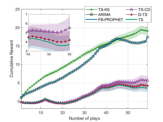
Figure 5: Cumulative reward vs number of plays [time window size = 30 days]

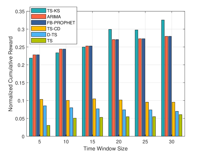
Figure 6: Time normalized cumulative reward vs time window size [in days]

We compare the performance of the proposed TS-KS algorithm with the different variants of Thompson sampling such as TS, dTS and TS-CD. In addition, we also compare TS-KS with state-of-the art forecasting algorithms such as ARIMA [34] and Facebook-PROPHET [35].

In particular, the ARIMA model considers that the output is linearly dependent on its own previous values and on an imperfectly predictable stochastic term. We select it for comparison since it is typically applied in cases where the data show evidence of non-stationarity in the sense of mean. Recently, in an attempt to develop a model that could capture seasonality in time-series data, Facebook developed the famous Facebook-PROPHET model that is publicly available. It is able to capture daily, weekly and yearly seasonality along with holiday effects, by implementing additive regression models. In essence, Facebook-PROPHET uses a piecewise linear model for trend forecasting. Its fitting procedure is usually very fast (even for thousands of observations) and it does not require any data pre-processing. It deals also with missing data and outliers. Due to its widespread popularity in time-series predictions, we select it as another competitor in our evaluation.

To facilitate the comparison, first, we consider a fixed window-size of 30 days and plot in Fig. 5 the temporal evolution of the reward over a period of about 5 years. Clearly, the TS-KS algorithm outperforms all the contending algorithms. In Fig. 5, we see a dip in the baseline algorithms (Facebook-PROPHET and ARIMA) during the phase when the portfolio with the highest valuation crashes (see Fig. 4). On the other hand, TS-KS is able to detect the change-points precisely and therefore has uniformly increasing cumulative reward. Then, from Fig. 6, we observe that the normalized cumulative reward is the maximum for TS-KS across all possible window-sizes varying from a week to a month. This establishes the efficacy of the proposed TS-KS algorithm vis-a-vis TS-CD and dTS.

Currently, we are investigating risk-constrained bandit algorithms in non-stationary environments, which we will report in a future work.

7 Conclusions and Future Work

We have proposed a KS-test based change detection mechanism for non-stationary environments in the MAB framework. Based on the KS-test, we have proposed an actively adaptive TS algorithm called TS-KS for the MAB problem. For the two-armed bandit case, the TS-KS algorithm has a sub-linear regret. It is noteworthy that the proposed framework is able to detect a change when the state-of-the-art mean-estimation based change detection mechanisms fail. Leveraging two case-studies, we have demonstrated that the TS-KS algorithm outperforms not only the classical TS and passively adaptive D-TS algorithms, but also it performs better than the actively adaptive TS-CD algorithm. Moreover, the performance of TS-KS is at par with the state-of-the-art forecasting algorithms such as Facebook-PROPHET and ARIMA as demonstrated in the portfolio optimization case study.

References

- [1] H. Mohanty, A. U. Rahman, and G. Ghatak. (2020) Thompson Sampling GoF. [Online]. Available: https://github.com/hardhik-99/Thompsom_Sampling_GoF/
- [2] D. Lee, N. He, P. Kamalaruban, and V. Cevher, “Optimization for reinforcement learning: From a single agent to cooperative agents,” IEEE Signal Processing Magazine, vol. 37, no. 3, pp. 123–135, 2020.
- [3] D. Bouneffouf and I. Rish, “A survey on practical applications of multi-armed and contextual bandits,” arXiv preprint arXiv:1904.10040, 2019.
- [4] P. Englert and M. Toussaint, “Combined optimization and reinforcement learning for manipulation skills.” in Robotics: Science and systems, vol. 2016, 2016.
- [5] G. Burtini, J. Loeppky, and R. Lawrence, “A survey of online experiment design with the stochastic multi-armed bandit,” arXiv preprint arXiv:1510.00757, 2015.
- [6] A. Lesage-Landry and J. A. Taylor, “The multi-armed bandit with stochastic plays,” IEEE Transactions on Automatic Control, vol. 63, no. 7, pp. 2280–2286, 2017.
- [7] S. Li et al., “Collaborative filtering bandits,” in Proceedings of the 39th International ACM SIGIR conference on Research and Development in Information Retrieval, 2016, pp. 539–548.
- [8] S. Buccapatnam, F. Liu, A. Eryilmaz, and N. B. Shroff, “Reward maximization under uncertainty: Leveraging side-observations on networks,” The Journal of Machine Learning Research, vol. 18, no. 1, pp. 7947–7980, 2017.
- [9] A. U. Rahman and G. Ghatak, “A beam-switching scheme for resilient mm-wave communications with dynamic link blockages,” in IEEE WiOpt, 2019.
- [10] Q. Zhu and V. Y. Tan, “Thompson sampling algorithms for mean-variance bandits,” arXiv preprint arXiv:2002.00232, 2020.
- [11] E. Contal, D. Buffoni, A. Robicquet, and N. Vayatis, “Parallel gaussian process optimization with upper confidence bound and pure exploration,” in Joint European Conference on Machine Learning and Knowledge Discovery in Databases. Springer, 2013, pp. 225–240.
- [12] W. R. Thompson, “On the likelihood that one unknown probability exceeds another in view of the evidence of two samples,” Biometrika, vol. 25, no. 3/4, pp. 285–294, 1933.
- [13] O.-C. Granmo, “Solving two-armed bernoulli bandit problems using a bayesian learning automaton,” International Journal of Intelligent Computing and Cybernetics, 2010.
- [14] S. Agrawal and N. Goyal, “Analysis of thompson sampling for the multi-armed bandit problem,” in Conference on learning theory, 2012, pp. 39–1.
- [15] A. Garivier and E. Moulines, “On upper-confidence bound policies for non-stationary bandit problems,” arXiv preprint arXiv:0805.3415, 2008.
- [16] O. Besbes et al., “Stochastic multi-armed-bandit problem with non-stationary rewards,” in Advances in neural information processing systems, 2014, pp. 199–207.
- [17] C. Hartland, S. Gelly, N. Baskiotis, O. Teytaud, and M. Sebag, “Multi-armed bandit, dynamic environments and meta-bandits,” 2006.
- [18] J. Y. Yu and S. Mannor, “Piecewise-stationary bandit problems with side observations,” in Proceedings of the 26th annual international conference on machine learning, 2009, pp. 1177–1184.
- [19] Y. Cao, Z. Wen, B. Kveton, and Y. Xie, “Nearly optimal adaptive procedure with change detection for piecewise-stationary bandit,” in The 22nd International Conference on Artificial Intelligence and Statistics, 2019, pp. 418–427.
- [20] O. Besbes et al., “Optimal exploration-exploitation in a multi-armed bandit problem with non-stationary rewards,” Stochastic Systems, vol. 9, no. 4, pp. 319–337, 2019.
- [21] J. Mellor and J. Shapiro, “Thompson sampling in switching environments with bayesian online change detection,” in Artificial Intelligence and Statistics, 2013, pp. 442–450.
- [22] V. Srivastava, P. Reverdy, and N. E. Leonard, “Surveillance in an abruptly changing world via multiarmed bandits,” in 53rd IEEE Conference on Decision and Control. IEEE, 2014, pp. 692–697.
- [23] G. Ghatak, “A change-detection based thompson sampling framework for non-stationary bandits,” IEEE Transactions on Computers, pp. 1–1, 2020.
- [24] P. Auer, P. Gajane, and R. Ortner, “Adaptively tracking the best bandit arm with an unknown number of distribution changes,” in Conference on Learning Theory, 2019, pp. 138–158.
- [25] S. S. Villar et al., “Multi-armed bandit models for the optimal design of clinical trials: benefits and challenges,” Statistical science: a review journal of the Institute of Mathematical Statistics, vol. 30, no. 2, p. 199, 2015.
- [26] K. Jahanbakhsh, “Applying multi-armed bandit algorithms to computational advertising,” arXiv preprint arXiv:2011.10919, 2020.
- [27] V. W. Berger and Y. Zhou, “Kolmogorov–smirnov test: Overview,” Wiley statsref: Statistics reference online, 2014.
- [28] P. Massart, “The tight constant in the dvoretzky-kiefer-wolfowitz inequality,” The annals of Probability, pp. 1269–1283, 1990.
- [29] S. Shalev-Shwartz and S. Ben-David, Understanding machine learning: From theory to algorithms. Cambridge university press, 2014.
- [30] N.-N. Dao, T.-T. Nguyen, M.-Q. Luong, T. Nguyen-Thanh, W. Na, and S. Cho, “Self-calibrated edge computation for unmodeled time-sensitive iot offloading traffic,” IEEE Access, vol. 8, pp. 110 316–110 323, 2020.
- [31] A. U. Rahman, G. Ghatak, and A. De Domenico, “An online algorithm for computation offloading in non-stationary environments,” IEEE Communications Letters, vol. 24, no. 10, pp. 2167–2171, 2020.
- [32] F. Black and R. Litterman, “Global portfolio optimization,” Financial analysts journal, vol. 48, no. 5, pp. 28–43, 1992.
- [33] D. Gawlik. (2017) New York Stock Exchange: S&P 500 companies historical prices with fundamental data. [Online]. Available: https://kaggle.com/dgawlik/nyse
- [34] H. A. Al-Zeaud, “Modelling and forecasting volatility using arima model,” European Journal of Economics, Finance & Administrative Science, vol. 35, pp. 109–125, 2011.
- [35] S. J. Taylor and B. Letham, “Forecasting at scale,” The American Statistician, vol. 72, no. 1, pp. 37–45, 2018.