Abstract

We adopt the interpretability offered by a parametric, Hawkes-process-inspired conditional probability mass function for the marks and apply variational inference techniques to derive a general and scalable inferential framework for marked point processes. The framework can handle both exchangeable and non-exchangeable event sequences with minimal tuning and without any pre-training. This contrasts with many parametric and non-parametric state-of-the-art methods that typically require pre-training and/or careful tuning, and can only handle exchangeable event sequences. The framework’s competitive computational and predictive performance against other state-of-the-art methods are illustrated through real data experiments. Its attractiveness for large-scale applications is demonstrated through a case study involving all events occurring in an English Premier League season.

1 INTRODUCTION

Point processes have been extensively used in a wide range of domains such as seismology (Hawkes, 1971; Hawkes and Oakes, 1974; Ogata, 1998), computational finance (Bacry et al., 2015, 2016), criminology (Mohler et al., 2011), examining insurgence in Iraq (Lewis et al., 2012), astronomy (Gregory and Loredo, 1992), neuroscience (Cunningham et al., 2007), sports (Gudmundsson and Horton, 2017) to name a few.

There is a voluminous literature on modelling event sequences with a vast proportion of it focusing on Hawkes process models (Hawkes, 1971) and their variants (Marsan and Lengline, 2008; Zhou et al., 2013; Iwata et al., 2013; Lemonnier and Vayatis, 2014; Hansen et al., 2015; Xu et al., 2016; Bacry and Muzy, 2016; Wang et al., 2016; Lee et al., 2016; Eichler et al., 2017; Yuan et al., 2019; Okawa et al., 2019; Zhang et al., 2020b; Donnet et al., 2020). Most of these methods are concerned with parametric forms of the intensity functions which generalize Hawkes processes. They aim to learn, non-parametrically, the so-called triggering kernels which model the dependencies between events. There are works where the whole conditional intensity function is learned non-parametrically based on Gaussian processes (Rasmussen and Williams, 2006), allowing the capture of complex events’ dynamics (Liu and Hauskrecht, 2019; Lloyd et al., 2016; Ding et al., 2018). Nevertheless, interpretability is further reduced in tandem with scalability due to the computationally demanding linear algebra required for training these models.

A more scalable solution that maintains flexibility and has produced state-of-the-art results is based on the introduction of deep learning techniques (Du et al., 2016; Mei and Eisner, 2017; Xiao et al., 2017; Li et al., 2018; Zhang et al., 2020a; Shchur et al., 2019). The majority of these methods model the intensity function of a point process through variants of recurrent neural networks (RNN). Recently, Shchur et al. (2019) has proposed a method that, instead of modelling the CIF, models the conditional distribution of the inter-arrival times using a log-normal mixture density network. Their model, though, assumes independence between occurrence times and marks, which is a strong assumption for the modelling of real-world event-sequence data. Interpretability in these methods is once again limited due to the black-box nature of the neural networks. Another class of models is Graphical event models (Didelez, 2008; Gunawardana et al., 2011; Bhattacharjya et al., 2018) where a graphical representation of multivariate point processes is used, offering interpretability but suffering from scalability issues due to their squared time complexity over the number of events. A recent work (Narayanan et al., 2021) introduced a new family of fully-parametric marked point processes, which provides both flexibility and interpretability through a decomposition of the joint distribution over times and marks, while the resulting model had directly interpretable parameterization. Nevertheless, the inference process has been based on a Hamiltonian Monte Carlo algorithm (Duane et al., 1987) in a high-dimensional space after a data wrangling procedure that eliminates parameter pre-training. Such an inference process quickly gets computationally prohibitive for large-scale event data sets.

Most of the aforementioned state-of-the-art (SOTA) methods for modelling event-sequence data are limited by the assumption of exchangeable event sequences. Despite the computational gains the exchangeability of event sequences delivers, such an assumption may considerably reduce the flexibility of the model, failing to capture complex dynamics between event sequences.

In this work, we inherit the interpretability offered by the conditional PMF for the marks in Narayanan et al. (2021), and we introduce an inferential framework based on variational inference (VI) (Blei et al., 2017) that successfully deals with the aforementioned scalability limitations. We also generalize the model through a latent autoregressive structure over the parameters, which relaxes the exchangeability assumption. The proposed model with the autoregressive component is general, and it could find various applications where the modelling of successive event sequences is required. We demonstrate the competitive performance of our VI framework against other SOTA baselines for marked point processes on a series of real-world datasets. We also use our method to extract valuable insights over the dynamics of association football teams using all events in a whole association football season, which is a substantially larger data set than Narayanan et al. (2021) considered. More importantly, the computational time is reduced to a few hours for data sets where Narayanan et al. (2021) would require several months of computation.

Our main contribution is a VI-based, scalable framework for modelling marked point processes with either exchangeable or non-exchangeable event sequences. Specifically, we provide the following:

• A scalable, general, VI-based inferential framework that can handle exchangeable and non-exchangeable event sequences requiring no pre-training parameter elimination and minimal tuning;

• Competitive performance against strong SOTA baselines (e.g. based on VI and deep learning) in terms of performance, facility of training, and interoperability;

• A large-scale case study of events from a whole association football season.

2 MARKED TEMPORAL POINT PROCESSES FOR EXCHANGEABLE EVENT SEQUENCES

2.1 Preliminaries

A marked temporal point process (MTPP) (Reinhart et al., 2018) can be seen as an ordered sequence of event times $t_{i}\in[0,T)$ over an observation interval $[0,T)$, accompanied by event marks $u_{i}\in\mathcal{U}$, which may include information about the event types or marks (discrete), location (continuous) or other event attributes. Our development focuses on discrete (multivariate temporal point process) mark spaces $\mathcal{U}$, however, extension to continuous spaces (marked spatiotemporal point process) is straightforward. An MTTP is fully determined by its conditional intensity function (CIF) $\lambda(t,u|\mathcal{F}_{t})$ which gives the probability of observing an event in the space $[0,T)\times\mathcal{U}$ given the filtration $\mathcal{F}_{t}=\{(t_{i},u_{i})\mid t_{i}<t\}$, i.e. $\lambda(t,u\mid\mathcal{F}_{t})~{}||B_{du}(u)||~{}dt=\mathbb{E}\left[N([t,t+dt]\times B_{du}(u))\mid\mathcal{F}_{t}\right]$, where $N(A)$ is the counting measure of events over the set $A\subseteq[0,T)\times\mathcal{U}$ and $||B_{du}(u)||$ is the Lebesgue measure over the open ball of radius $du>0$ in $\mathcal{U}$. Given a dataset $\mathcal{D}=\{\mathbf{y}_{s}\}_{s=1}^{S}$, where $\mathbf{y}_{s}=\{(t_{i}^{(s)},u_{i}^{(s)})\}_{i=1}^{N_{s}}$ is the $s$th event sequence consisting of $N_{s}$ time-mark pairs $(t_{i}^{(s)},u_{i}^{(s)})$, and under an exchangeability assumption about the event sequences, the log-likelihood of $\mathcal{D}$ is written as

$$\mathcal{L}(\mathcal{D})=\sum_{s=1}^{S}\ell_{s},$$ (1)

where the log-likelihood of each sequence $s$ is $\ell_{s}=\sum_{i=1}^{N_{s}}\log\lambda(t_{i}^{(s)},u_{i}^{(s)}\mid\mathcal{F}_{t_{i}^{(s)}})-\int_{0}^{T}\int_{\mathcal{U}}\lambda(t,u\mid\mathcal{F}_{t^{(s)}})dudt$. $\mathcal{F}_{t^{(s)}}=\{(t_{i}^{(s)},u_{i}^{(s)})\mid t_{i}^{(s)}<t^{(s)}\}$ is the filtration of the $s$th sequence; the dependence of $\ell_{s}$ on the parameters and the data has suppressed for notational convenience. In what follows, we also suppress the dependence on the $s$-th sequence to reduce clutter in the notation, unless otherwise stated. Multivariate Hawkes process Hawkes (1971) is a well-studied MTPP, where past events contribute additively to the intensity of the current event, allowing in that way to capture mutual excitation (clustering) behaviour between events. The CIF of a multivariate Hawkes process with mark space $\mathcal{U}=\{1,\cdots,U\}$ is given by

$$\lambda(t,u\mid\mathcal{F}_{t}) =\mu\delta_{u}+\eta\sum_{j:t_{j}<t}\beta_{u_{j},u}e^{-\beta_{u_{j},u}(t-t_{j})}\gamma_{u_{j},u},$$ (2)

where $\mu>0$ is a constant background intensity, $\delta_{u}>0$ is the background probability for event type $u$ with $\sum_{u=1}^{U}\delta_{u}=1$, $\gamma_{u_{j},u}>0$ is the probability of triggering an event type $u$ from the excitation of an event type $u_{j}$ where $\sum_{u=1}^{U}\gamma_{u_{j},u}=1$, $\forall u_{j}\in\mathcal{U}$, while $\beta_{u_{j},u}>0$ is the exponential decay rate of that excitation. The parameter $\eta\in(0,1)$ is called the excitation factor.

2.2 Decoupled MTPP

Despite their widespread applicability in modelling event sequences (Ogata, 1981; Mohler et al., 2011; Bowsher, 2007), Hawkes processes perform poorly in cases where event times do not exhibit clustering behavior. An example of such a setting is football event sequences, where the inter-arrival times tend to be under-dispersed relative to a Poisson process which is the limit of a Hawkes process when $\eta$ in (2) approaches zero. The drawbacks of Hawkes processes in this setup are discussed in Section 3.3 of Narayanan et al. (2021). These limitations are circumvented by considering the decomposition of the log-likelihood of a marked point process,

$$\ell=\sum_{i=1}^{N} \left\{\log f(u_{i}\mid t_{i},\mathcal{F}_{t_{i}};\boldsymbol{\theta}_{f})+\log g(t_{i}\mid\mathcal{F}_{t_{i}};\boldsymbol{\theta}_{g})\right\}$$

$$+\log\left(1-G(T\mid\mathcal{F}_{t_{N}};\boldsymbol{\theta}_{g})\right),$$ (3)

where $f(\cdot|\cdot~{};\boldsymbol{\theta}_{f})$ and $g(\cdot|\cdot~{};\boldsymbol{\theta}_{g})$ are the conditional probability mass function (PMF) of the event types and the conditional density for the occurrence times, respectively, parameterized by vectors $\boldsymbol{\theta}_{f}$ and $\boldsymbol{\theta}_{g}$, and $G(u\mid\cdot)=\int_{0}^{u}g(t\mid\cdot)dt$. The last term in (2.2) is the logarithm of the survival function that accounts for the fact that the unobserved occurrence time $t_{N+1}$ must be after the end of the observation interval $(0,T)$. The dependence of $\ell$ in (2.2) on $\boldsymbol{\theta}_{f}$ and $\boldsymbol{\theta}_{g}$ has been suppressed to simplify notation and it is omitted henceforth in $f(\cdot\mid\cdot)$ and $g(\cdot\mid\cdot)$ unless required. All likelihood contributions in  (2.2) share the same parameters $\boldsymbol{\theta}_{f}$ and $\boldsymbol{\theta}_{g}$, which, in turn, are assumed to have prior distributions. Therefore, the event sequences are independent conditional on $\boldsymbol{\theta}_{f}$ and $\boldsymbol{\theta}_{g}$, and, hence, exchangeable but not necessarily marginally independent. See, for example, Section 1 in Blei et al. (2003) for a discussion about the concept of exchangeability.

This decomposition allows defining an MTPP in terms of $f(\cdot\mid\cdot)$ and $g(\cdot\mid\cdot)$ instead of the CIF $\lambda(t,u\mid\mathcal{F}_{t})$, providing extra flexibility to the specification of the model, and thus, added expressibility. For example, a gamma or a log-normal density could be chosen as $g(\cdot\mid\cdot)$ to capture non-clustering relations among time occurrences, like under-dispersion.

In the current work, we adopt the same functional form of $f(u_{i}\mid t_{i},\mathcal{F}_{t_{i-1}})$ as in Narayanan et al. (2021), i.e.

$$f(u_{i}|t_{i},\mathcal{F}_{t_{i}})=\frac{\delta_{u_{i}}+\eta\sum_{j:t_{j}<t_{i}}\gamma_{u_{j},u_{i}}e^{-\beta_{u_{j},u_{i}}(t_{i}-t_{j})}}{1+\eta\sum_{j:t_{j}<t_{i}}e^{-\beta_{u_{j},u_{i}}(t_{i}-t_{j})}},$$ (4)

where $\eta>0$. Expression (4) is obtained by converting (2) into a PMF by normalising across all possible values of $u$. We define the probability vector $\boldsymbol{\delta}=(\delta_{1},\cdots,\delta_{U})^{\top}$, the stochastic matrix $\Gamma\in[0,1]^{U\times U}$ with $\Gamma_{u,u^{\prime}}=\gamma_{u,u^{\prime}}$, the decay matrix $B\in\mathbb{R}_{+}^{U\times U}$ where $B_{u,u^{\prime}}=\beta_{u,u^{\prime}}$. Hence, the model parameters are $\boldsymbol{\theta}_{f}=\{\boldsymbol{\delta},\Gamma,B,\eta\}$.

The PMF of marks in (4) possesses a natural interpretation of its parameters. Large values of $\eta$ correspond to higher dependence of each mark on its past events since $\eta$ can be viewed as a scaling factor over the contributions of past events to the current event mark probability. The probabilities $\gamma_{u_{j},u}$ can be interpreted as the conversion rates for the transition from an event type $u_{j}$ to an event type $u$ while the decay rate $\beta_{u,u^{\prime}}$ quantifies the exponential rate at which the excitation from a previous event with mark $u$ decays over time given the current event with mark $u^{\prime}$. The background probability $\delta_{u}$ gives the probability an event has a mark $u$ given this event is triggered exclusively by a background process. In this way, we can extract useful information regarding the cross-excitations between the event types and the corresponding excitation decay rates.

2.3 Proposed Model for Exchangeable Event Sequences

Despite the flexibility of (4), the implementation in Narayanan et al. (2021) is based on an MCMC algorithm that scales poorly with the number of time events after a data wrangling procedure that eliminates parameter pre-training, thus limiting its applicability only to small data sets. We address this limitation through a VI implementation strategy that maintains the desirable properties of the model in Narayanan et al. (2021), such as producing approximate posterior distributions over the parameters, while delivering vast computational speed-up over its MCMC counterpart. We focus on the PMF in (4), which, despite all the interpretability that brings into the model, is the computational bottleneck for the inference process.

Variational inference.

By considering a variational distribution $q_{\boldsymbol{\xi}}(\boldsymbol{\theta}_{f})$, parameterized by the variational parameters $\boldsymbol{\xi}$, we aim to find these parameters that minimize the Kullback-Leibler divergence between the variational distribution $q_{\boldsymbol{\xi}}(\boldsymbol{\theta}_{f})$ and the true posterior $p_{\boldsymbol{\xi}}(\boldsymbol{\theta}_{f}|\mathcal{D})$. This is equivalent to maximizing the evidence lower bound (ELBO) (Blei et al., 2017; Zhang et al., 2018) defined as

$$\text{ELBO}(\boldsymbol{\xi},\boldsymbol{\nu}):=\mathbb{E}_{q_{\boldsymbol{\xi}}}\left[\log\frac{p(\mathcal{D}\mid\boldsymbol{\theta}_{f})p_{\boldsymbol{\nu}}(\boldsymbol{\theta}_{f})}{q_{\boldsymbol{\xi}}(\boldsymbol{\theta}_{f})}\right],$$ (5)

where $p(\mathcal{D}|\boldsymbol{\theta}_{f}):=\prod_{s=1}^{S}\prod_{i=1}^{N_{s}}f(u_{i}^{(s)}\mid t_{i}^{(s)},\mathcal{F}_{t_{i}}^{(s)};\boldsymbol{\theta}_{f})$ is the data likelihood, and $p_{\boldsymbol{\nu}}(\boldsymbol{\theta}_{f})$ is the prior with hyperparameters $\boldsymbol{\nu}$, which are also chosen to maximize ELBO.

Regarding the variational distribution $q_{\boldsymbol{\xi}}(\boldsymbol{\theta}_{f})$, we follow the mean-field approach where $q_{\boldsymbol{\xi}}$ factorizes over $\boldsymbol{\theta}_{f}$, i.e. $q_{\boldsymbol{\xi}}(\boldsymbol{\theta}_{f})=q_{\boldsymbol{\xi}}(\boldsymbol{\delta})q_{\boldsymbol{\xi}}(\Gamma)q_{\boldsymbol{\xi}}(B,\eta)$, where each constituent distribution is defined as

$$q_{\boldsymbol{\xi}}(\boldsymbol{\delta})=\text{Dir}(\boldsymbol{\alpha}_{0}),\quad q_{\boldsymbol{\xi}}(\Gamma)=\prod_{u=1}^{U}\text{Dir}(\boldsymbol{\alpha}_{u}),$$ (6)

$$q_{\boldsymbol{\xi}}(B,\eta)=\prod_{p=1}^{U^{2}+1}\text{Lognormal}(\mu_{p},\sigma^{2}_{p}).$$ (7)

In the above expressions, $\boldsymbol{\alpha}_{p}\in\mathbb{R}_{+}^{U},p=0,1,\cdots,U$ are the concentration parameters of each Dirichlet distribution and $\{\mu_{p},\sigma^{2}_{p}\}_{p=1}^{U^{2}+1}$ are the means and variances of the log-normal distributions, and thus, $\boldsymbol{\xi}=\{\{\boldsymbol{\alpha}_{p}\}_{p=0}^{U},\{\mu_{p},\sigma^{2}_{p}\}_{p=1}^{U^{2}+1}\}$.

In order to maximize ELBO with respect to both $\boldsymbol{\xi},\boldsymbol{\nu}$, we adopt a similar procedure as in Salehi et al. (2019) where a variational EM algorithm is employed to iteratively optimize (5). For calculating ELBO, we refer to black-box variational inference (BBVI) optimization (Ranganath et al., 2014; Kingma and Welling, 2013) where Monte Carlo integration is used to approximate the bound. The reparameterization trick in Kingma and Welling (2013) allows us to obtain unbiased gradient estimates of the ELBO for the parameters of the log-normal distributions in (7). However, the reparameterization trick is not applicable to the concentration parameters $\boldsymbol{\alpha}_{i}$. To overcome this issue, we make use of pathwise gradients (Jankowiak and Obermeyer, 2018), allowing us to obtain an estimate of ELBO, given by

$$\text{ELBO}(\boldsymbol{\xi},\boldsymbol{\nu})\approx\frac{1}{L}\sum_{l=1}^{L}\log\frac{p(\mathcal{D}\mid\boldsymbol{\theta}^{(l)}_{f})p_{\boldsymbol{\nu}}(\boldsymbol{\theta}^{(l)}_{f})}{q_{\boldsymbol{\xi}}(\boldsymbol{\theta}^{(l)}_{f})},$$ (8)

for $L$ Monte Carlo samples $\boldsymbol{\theta}^{(l)}_{f}$ generated from the variational distribution using the reparameterization trick/pathwise gradients. Following Salehi et al. (2019), we maximize (8) with respect to the variational parameters $\boldsymbol{\xi}$ in the E-step while in the M-step we maximize with respect to the hyperparameters $\boldsymbol{\nu}$. The updated $\boldsymbol{\nu}$ can be found in closed form when certain priors are utilized (Salehi et al., 2019). In this work, we consider a zero-mean Gaussian prior over $\eta$ and the entries of $B$, and thus, we need $U^{2}+1$ hyperparameters to describe them. Furthermore, by imposing Dirichlet priors over $\Gamma$ and $\boldsymbol{\delta}$, updating the concentration parameters of these priors is not required. This can be seen by writing

$$\mathbb{E}_{q_{\boldsymbol{\xi}}}\left[\log\frac{p(\mathcal{D}\mid\boldsymbol{\theta}_{f})p_{\boldsymbol{\nu}}(\boldsymbol{\theta}_{f})}{q_{\boldsymbol{\xi}}(\boldsymbol{\theta}_{f})}\right]$$

$$=\mathbb{E}_{q_{\boldsymbol{\xi}}}\left[\log p(\mathcal{D}\mid\boldsymbol{\theta}_{f})\right]-\text{KL}[q_{\boldsymbol{\xi}}(\boldsymbol{\theta}_{f})\mid\mid p_{\boldsymbol{\nu}}(\boldsymbol{\theta}_{f})],$$

where $\text{KL}[q||p]$ is the Kullback-Leibler (KL) divergence between distribution $q$ and $p$. The above expression is maximized when the KL divergence is zero, which is true for two Dirichlet distributions when they share the same concentration parameters. Hence, these Dirichlet priors can be safely ignored from the ELBO and no hyperparameter update is required at the M-step. Details on the derivation of ELBO and the optimization procedure can be found in Section A of Appendix.

Computational speed-up.

The above model, despite its flexibility, still suffers from scalability issues due to the log-likelihood term $\log p(\mathcal{D}\mid\boldsymbol{\theta}_{f})$ which scales as $\mathcal{O}(SN^{2})$ where $N=\max_{s=1,\cdots,S}|\mathbf{y}_{s}|$. To circumvent the problem, we assume that past events do not contribute to the evaluation of the summation term in (4) up to a point, and thus, they can be ignored from the computation. Specifically, we use the following assumptions (Liu and Hauskrecht, 2019):

Assumption 1.

$\forall u=1,\cdots,U$, $\exists B_{u}>0$ such that if $0<B_{u}<t_{i}-t_{u}$, where $t_{u}\in\{t_{j}>0:t_{j}<t_{i},~{}u_{j}=u\}$ then these events do not contribute to the sum in (4).

Assumption 2.

$\forall u=1,\cdots,U$, $\exists~{}C_{u}:\mathbb{R}_{>0}\rightarrow\mathbb{N}$ such that for any finite interval $\mathcal{A}=[t_{\rm start},t_{\rm end}),|\mathcal{A}|=t_{\rm end}-t_{\rm start}$, the number of events of type $u$ in this interval $\mathcal{N}_{u}(\mathcal{A})$ are bounded above by $C_{u}(|\mathcal{A}|)<\infty$.

Theorem 1 (Proof in Liu and Hauskrecht (2019)).

Under assumptions 1 and 2, $\exists~{}Q\in\mathbb{N}$ such that the sum in (4) only requires the last $Q$ events of $\mathcal{F}_{t_{i}}$.

Theorem 1 allows us to reduce the time complexity to $\mathcal{O}(SQN)$ rendering inference feasible for large-scale datasets. This assumption can be justified by the fact that large time intervals $t_{i}-t_{j}$ lead to near to zero contributions for past events $t_{j}$ in (4), and hence, their absence would not affect the final log-likelihood value. $Q$ is a tunable hyperparameter that can be determined by inspecting the values of the log-likelihood on a validation dataset. Similar cut-off assumptions to speed up computations have been also considered in Liu and Hauskrecht (2019) and Zhang et al. (2020b), while a Bayesian treatment is considered in Linderman and Adams (2015).

The overall complexity is affected by the number of Monte Carlo samples $M$. However, $M=1$ is usually sufficient for BBVI applications as previous studies indicate (Kingma and Welling, 2013; Salehi et al., 2019). Finally, to further reduce the computational burden, we approximate the log-likelihood (1) by randomly selecting batches of sequences $\mathcal{B}\subseteq\{1,2,\cdots,S\}$, and taking unbiased estimates $\sum_{s=1}^{S}\ell_{s}\approx S\sum_{s^{\prime}\in\mathcal{B}}\ell_{s^{\prime}}/|\mathcal{B}|.$

Time modelling.

Time occurrences are modelled by log-normal distributions, i.e. $g(t_{i}\mid\mathcal{F}_{t_{i}};\boldsymbol{\theta}_{g})=p(r_{i}\mid u_{i-1},\tilde{\boldsymbol{\mu}},\tilde{\boldsymbol{\sigma}})$, where $r_{i}:=t_{i}-t_{i-1}$, $t_{0}=0$, $\tilde{\boldsymbol{\mu}}\in\mathbb{R}^{U},~{}\tilde{\boldsymbol{\sigma}}\in\mathbb{R}^{U}_{+}$ are the means and standard deviations of the log-normal distributions, respectively, with density $p(r_{i})$. Therefore, the inter-arrival times $r_{i}$ are log-normally distributed where the distribution’s parameters depend on the value of the previous mark $u_{i-1}$, i.e. $r_{i}\sim\text{Lognormal}(\tilde{\mu}_{u_{i-1}},\tilde{\sigma}_{u_{i-1}}^{2})$. In a similar way, we could consider any continuous distribution with support on the positive reals for the inter-arrival times, such as gamma. However, we found that log-normal distributions are sufficient for the real-world datasets considered in Section 2.4. Note also that the distribution over inter-arrival times allows for the easy and fast prediction of the time of future events. This is in contrast to prediction for CIF-based models, which requires computationally demanding procedures, like Ogata’s modified thinning algorithm (Ogata, 1981). Specifically, for a point process with CIF $\lambda(t)$, a prediction of the next time occurrence $t^{*}$ is computed as f $t^{*}=\mathbb{E}[\tilde{t}|\mathcal{F}_{t}]=\int_{t}^{\infty}\tilde{t}~{}\lambda(\tilde{t}\mid\mathcal{F}_{t})~{}\exp\left(-\int_{t}^{\tilde{t}}\lambda(u\mid\mathcal{F}_{t})du\right)d\tilde{t}$, which is intractable, and Monte Carlo sampling via Ogata’s algorithm is used to estimate it. In our formulation, we simply use the mode of the log-normal distribution to predict the next time occurrence.

2.4 Experiments on Real-World Data

We investigate the predictive performance of the proposed model under the exchangeability assumption in the previous section, which we term VI-Decoupled Point Process (VI-DPP), over four real-world datasets and compare the results to state-of-the-art baselines. Our code, based on PyTorch (Paszke et al., 2019), is available at https://github.com/aresPanos/Interpretable-Point-Processes.

We consider four real-world datasets with a range of characteristics, such as the number of sequences $S$, total number of events, mean sequence length etc; see Table 4 in Appendix. A detailed description of each of the datasets can be found in Section C of Appendix. Our method is trained on these four datasets and results are compared to those of three other baselines. We pick, for comparison, the VI-based Hawkes process variant in Salehi et al. (2019) due to its state-of-the-art performance over other MLE-based methods. We use both a parametric version with an exponential triggering function (VI-EXP) and a non-parametric one with a mixture of Gaussians triggering function (VI-SG). This method resembles ours in the way that inference is performed, however, it is limited to a parameterized form of a Hawkes process CIF and it requires careful hyperparameter tuning which is usually computationally demanding for large-scale applications. We also include in our comparisons the Self-Attentive Hawkes Process (SAHP) (Zhang et al., 2020a), which is the state-of-the-art NN-based method that uses the self-attention mechanism (Vaswani et al., 2017) to address the effect of long-range/non-linear dependencies. Note that comparison with the STAN HMC implementation in Narayanan et al. (2021) is infeasible to the real-world datasets and the case study in Section 3.2 due to extremely high running times; see pages 80, 98 of Narayanan (2020).

Table 1: Performance comparison between our proposed model (VI-DPP) and three other baselines over the four real-world datasets of Section 2.4. The best results across the four competing approaches are in bold.

Methods	Metrics	Mimic		SOF		Mooc		Ret
	LLKL	-3.072	(0.148)	-2.523	(0.022)	-1.387	(0.024)	-0.733	(0.005)
VI-EXP	RMSE	3.075	(0.897)	71.175	(9.970)	112.805	(6.951)	332.604	(83.590)
	$F_{1}$	82.28	(5.54)	5.52	(0.60)	10.10	(0.38)	41.21	(0.52)
	Time (min)	116.53	(15.29)	99.92	(21.78)	842.44	(133.20)	67.19	(10.85)
	LLKL	-3.070	(0.144)	-2.461	(0.022)	-4.260	(0.041)	0.238	(0.011)
VI-Gauss	RMSE	5.190	(1.817)	53.778	(10.098)	5436.984	(486.614)	319.599	(37.234)
	$F_{1}$	80.77	(4.59)	5.64	(0.86)	5.57	(0.41)	40.78	(0.82)
	Time (min)	248.94	(118.58)	586.13	(49.86)	1400.96	(128.93)	61.57	(17.65)
	LLKL	1.534	(0.215)	-0.506	(0.006)	1.289	(0.136)	0.621	(1.670)
SAHP	RMSE	10.896	(2.447)	44.968	(4.450)	28.409	(12.342)	354.880	(26.162)
	$F_{1}$	63.60	(6.38)	8.45	(0.31)	14.07	(0.95)	41.31	(0.70)
	Time (min)	63.09	(1.64)	398.21	(21.17)	528.34	(26.81)	80.54	(24.70)
	LLKL	-2.520	(0.103)	-2.483	(0.025)	-0.369	(0.014)	1.063	(0.020)
VI-DPP	RMSE	0.969	(0.043)	5.508	(1.235)	0.997	(0.000)	1.000	(0.000)
	$F_{1}$	57.42	(3.82)	10.04	(0.24)	19.52	(1.04)	41.15	(0.07)
	Time (min)	3.45	(0.17)	83.99	(6.03)	127.32	(1.98)	682.23	(2.05)

We randomly split each dataset into ten train/validation/test ($70\%/10\%/20\%$) sets. The train data set is used for inference, the validation dataset is used for tuning the hyperparameters, and the predictive performance is evaluated on the test dataset. Predictive performance is assessed by three different metrics: (i) mean log-likelihood (LLKL) for the ability of each method to model event sequences, (ii) root-mean-square error (RMSE) for the ability of each method to predict future time events, and (iii) $F_{1}$ score for the ability of each method to predict future marks. RMSE is computed as in Zhang et al. (2020a), i.e. the square root of the sum of the squares of $\epsilon_{i}=(t_{i+1}^{*}-t_{i})/(t_{i+1}-t_{i})-1$, where $t_{i+1}^{*}$ is the predicted time of the next event. $F_{1}$ score is chosen to take into account possible mark imbalances. Regarding mark prediction, since our VI method gives a distribution over the parameters $\boldsymbol{\theta}_{f}$ and not a point estimate, the PMF in (4) is computed using the mode of the log-normal distribution in (7) and the mean of the Dirichlet distributions in (6); see Table 1 and more details in Section B of Appendix.

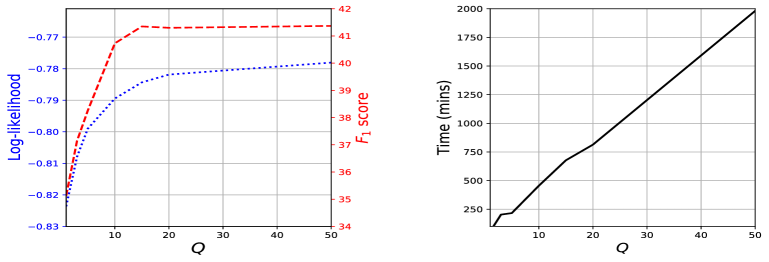
Figure 3: The values of log-likelihood (left panel, blue dotted line), $F_{1}$ score (left panel, red dashed line), and training time (right panel, black solid line) as a function of the number of cut-off points $Q$ for our model VI-DPP trained over the Retweet dataset. The log-likelihood computation here takes into account only the marks.

We see that VI-DPP consistently outperforms the other baselines in terms of both RMSE and $F_{1}$, providing evidence for the flexibility of the decoupled MTPP. SAHP scores higher values of LLKL due to the flexibility of the NN which is based on. The superior performance of VI-DPP compared to the other methods in RET, MIMIC, and MOOC is due to the fact that these datasets have small inter-arrival times (or zero, to which we have to add a small positive constant as Zhang et al. (2020a) do in their codebase) and/or large heterogeneity in those, resulting in either small sample means $\hat{\mu}$ of the log of the inter-arrival times and/or high variance $\hat{\sigma}^{2}$ of those. Hence, our mark-specific conditional log-normal models for the inter-arrival times are often trained to have modes that are very close to zero (the estimated mode of the log-normal is $\exp(\hat{\mu}-\hat{\sigma}^{2})$, which results in test RMSE that is very close to 1. We also notice a significant speed-up of our method over the rest competitors for all datasets but the Retweets. This is because a small number of cut-off points $Q$ is enough to achieve good results for the first three datasets while for Retweet a larger $Q$ is required; see Section B of Appendix. It is worth mentioning that our method required minimal hyperparameter tuning in contrast to the other three baselines where meticulous hyperparameter tuning was crucial for achieving competitive results. This process leads to considerably higher computational times, especially for large-scale datasets, something that is not directly revealed in Table 1. Fig. 3 of Appendix explores how $Q$ affects the performance of our model in terms of RMSE, $F_{1}$ score, and training time over the Retweets dataset. Values of $Q>20$ do not provide any significant performance boost for both RMSE and $F_{1}$, while training time, as expected, increases linearly with respect to $Q$. Ignoring events in the far past, as we do for our method, cannot be applied to SAHP due to its dependence on the self-attention mechanism, and it would not improve the VI-EXP and VI-GAUSS training times because of their pre-processing steps.

Table 2: Size of the association football dataset (leftmost table) and a performance comparison between our proposed model (VI-DPP) and three other baselines on the same dataset (rightmost table).

# of teams	20
# of games	380
# of sequences	760
# of events	524,160
$U$	30

	VI-EXP	VI-Gauss	SAHP	THP	VI-DPP
RMSE	15.6430	14.9554	0.7206	0.6754	0.4855
$F_{1}$	2.43	2.40	5.64	16.98	18.73
Time (min)	203.77	145.61	>1200	>1200	139.91

3 NON-EXCHANGEABLE EVENT SEQUENCES

3.1 Relaxing Exchangeability

We can relax the assumption of exchangeable event sequences in (2.1) by making one or more of the parameters in $\alpha,\boldsymbol{\delta},\Gamma,B$ in (4) depend on the event sequences or on a set of event sequences. Then, we can assume autoregressive latent processes for those parameters. Here, we focus on placing autoregressive latent processes on the conversion rates $\Gamma$ because of the facility to incorporate process- or event-specific covariate information whose effect is directly interpretable in terms of log-odds of triggering an event type from the excitation of another event type.

The event-sequence-specific conversion rates can be linked to covariate vectors $(x_{t1},\ldots,x_{tp})^{\top}$ observed at time $t$ by letting

$$\log\frac{\gamma_{u,u^{\prime}}(t^{(s)})}{\gamma_{u,U}(t^{(s)})}=\phi_{u,u^{\prime}}+\sum_{j=1}^{p}\omega_{ju^{\prime}}^{(s)}x_{t^{(s)}j},$$

$\forall~{}u^{\prime}\in\{1,\cdots,U-1\},u\in\{1,\cdots,U\}$. We then assume that the covariate effects follow independent autoregressive processes with $\omega_{ju^{\prime}}^{(1)}\sim\mathcal{N}(\mu_{ju^{\prime}},~{}\sigma_{ju^{\prime}}^{2}/(1-\rho_{ju^{\prime}}^{2}))$ and $\omega_{ju^{\prime}}^{(s)}\mid\omega_{ju^{\prime}}^{(s-1)}\sim\mathcal{N}(\mu_{ju^{\prime}}+\rho_{ju^{\prime}}\omega_{ju^{\prime}}^{(s-1)},~{}\sigma_{ju^{\prime}}^{2})$ $(s=2,\ldots,S)$. The log-likelihood is given by

$$\log\int_{\boldsymbol{\omega}}\prod_{s=1}^{S}~{}\mathcal{L}^{(s)}(\mathcal{F}^{(s)},\boldsymbol{\omega}^{(s)})~{}dP(\boldsymbol{\omega}),$$ (9)

which, in contrast to (1), is not tractable because we need to integrate out the latent parameters. $\mathcal{L}^{(s)}(\mathcal{F}^{(s)},\boldsymbol{\omega}^{(s)})$ is the event-type likelihood from all events in the $s$-th event sequence defined by the mass function in (4), and $\mathcal{F}^{(s)}$ is all the information available up to and including the $s$-th event sequence. The prior probability measure $P(\boldsymbol{\omega})$ is a $p\times(U-1)\times S$-dimensional Gaussian measure with mean vector defined by $\mu_{ju^{\prime}}$ and covariance matrix fully described by $\rho_{ju^{\prime}}$ and $\sigma_{ju^{\prime}}$; more details about autoregressive processes can be found in Section 2 of Rue and Held (2005). The logarithm is outside the integral in (9), making its computation numerically unstable. Hence, we resort to Jensen’s inequality to obtain a lower bound on (9),

$$\sum_{s=1}^{S}~{}\int_{\boldsymbol{\omega}^{(s)}}~{}\log\left(\mathcal{L}^{(s)}(\mathcal{F}^{(s)}\mid\boldsymbol{\omega}^{(s)})\right)~{}dP(\boldsymbol{\omega}^{(s)}),$$ (10)

which holds due to logarithm properties and conditional independence of $\omega_{ju^{\prime}}^{(s)}$. By treating $\{\mu_{ju^{\prime}},~{}\sigma_{ju^{\prime}},~{}\rho_{ju^{\prime}}\}$ as hyperparameters, we can naturally apply the VI framework of Section 2.3 by plugging (10) into (8) and maximize the new variational lower bound with respect to hyperparameters, the variational parameters, and the whole vector $\boldsymbol{\omega}$, and thus, deriving an approximation over the posterior mode of $\boldsymbol{\omega}$ given all the association football data.

Notice that the ELBO is regularized by the log-Gaussian density over the latent $\boldsymbol{\omega}$. The optimization procedure is now identical to the one followed in Section 2.3 while the assigned variational densities and priors for $\boldsymbol{\theta}_{f}=\{\boldsymbol{\delta},\Gamma,B,\eta\}$ hold the same as well. The $p\times(U-1)$-dimensional Gaussian integrals in (10) are approximated by Monte Carlo integration since the convenient structure of the inverse covariance matrix of an autoregressive process allows sampling with linear time complexity (Rue and Held, 2005).

As is done in the application of the next section, the above applies unaltered if the non-exchangeable event sequences are replaced by non-exchangeable sets of event sequences.

3.2 Association Football Data

Over the last decade, the importance of analysing association football matches, in tandem with the availability of spatiotemporal data from these matches, have sparked the development of many research works focusing on the statistical modelling of teams’ and/or players’ performance. Recent works on the analysis of spatiotemporal data from team sports, such as football, have been developed with a primary focus on each player’s performance or the pattern extraction in the team plays. These works use for their analysis, as we do in this section, event data streams from various team sports where each event can be fully described by the occurrence time, its location, its type (goal, pass, etc.), and the involved players, and team information. For instance, Passos et al. (2011); Grund (2012); Duch et al. (2010); Clemente et al. (2015) focus on modelling player interaction through network analysis. Other works aim to identify patterns from pass sequences (Wang et al., 2015; Van Haaren et al., 2016) or other patterns that lead to a goal event (Decroos et al., 2017).

Another stream of literature relies on the extraction of game states from event sequences in order to numerically assess in-game player actions (Routley and Schulte, 2015; Decroos et al., 2019) or to predict goal probabilities given the current game state (Robberechts et al., 2019). Gudmundsson and Horton (2017) provides a detailed survey of the use of spatiotemporal analysis in team sports. A more recent work (Narayanan et al., 2021) followed a different direction where they studied the dynamics of association football matches by modelling all event sequences within a game through a marked point process. The framework in Narayanan et al. (2021) relies on MCMC in a high-dimensional space after a data wrangling procedure that eliminates parameter pre-training, and can only handle exchangeable event sequences like most of the state-of-the-art (SOTA) methods for modelling event-sequence data. This poses severe computational and conceptual limitations in the realistic modelling of large-scale event-sequence data.

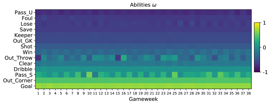
Figure 1: Values of Spearman’s rank correlation coefficient between $\omega_{\cdot,u^{\prime}}^{(w)}\in\mathbb{R}^{20},~{}w=1\cdots,38$, for each event type $u^{\prime}$ and the accumulated points awarded to each team at the end of the season, throughout the 38-week season.

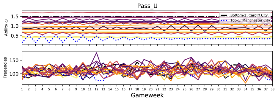
Figure 2: Top panel shows the evolution of unsuccessful passes (Pass_U) ability $\omega_{c,3}^{(t)}$ for each team across the season while the bottom one illustrates the same information using the raw frequencies of Pass_U from the association football dataset. The blue and black dashed lines correspond to Manchester City and Cardiff, the winner and bottom-ranked teams of the 2013/2014 Premier league respectively. The colors for the rest of the teams have been assigned according to their final rank, with brighter colors associated with teams with higher ranks at the end of the championship.

The data used in this study consists of all touch-ball events recorded in all English Premier League (EPL) games throughout the season 2013/2014. Each sequence includes the touch events from one of the two halves of each game. Hence, we have 760 sequences for 380 games between 20 teams for the season and more than half a million touch-ball events. The dataset consists of triplets $(t,u,z)$, where $t$ is the time when the touch-ball event occurred, $u$ is the event type with $u\in\{1,\ldots,30\}$ and $z\in\{1,2,3\}$ denotes the spatial location, or zone, in the football field that the event took place. There are 15 distinct types labeled by which team (home or away) triggered the event; see Table 3 in Appendix and Narayanan et al. (2021) for a detailed description of the data and pre-processing steps.

In association football, the process ends immediately after the last event in each half of the game. Hence, the last term in (2.2) is not part of the likelihood; see Section 4.2 of Lindqvist (2006).

We consider a generalization of (4) from Narayanan et al. (2021) where

$$f(u_{i}|t_{i},z_{i},\mathcal{F}_{t_{i}})=\frac{\delta_{u_{i}}^{z_{i}}+\alpha\sum_{j:t_{j}<t_{i}}\gamma_{u_{j},u_{i}}^{z_{i}}e^{-\beta_{u_{j},u_{i}}^{z_{i}}(t_{i}-t_{j})}}{1+\alpha\sum_{j:t_{j}<t_{i}}e^{-\beta_{u_{j},u_{i}}^{z_{i}}(t_{i}-t_{j})}},$$ (11)

that accounts for the zone information.

The parameters $\boldsymbol{\delta},\Gamma,B$ are now location specific, i.e. $\boldsymbol{\delta}^{z}_{u}=\delta_{u}^{z},\Gamma^{z}_{u,u^{\prime}}=\gamma_{u,u^{\prime}}^{z}$, and $B^{z}_{u,u^{\prime}}=\beta_{u,u^{\prime}}^{z}$. Team information is incorporated in the model via the baseline-category logit representation $\log\{\gamma_{u,u^{\prime}}^{z}(t)/\gamma_{u,U}^{z}(t)\}=\phi_{u,u^{\prime}}^{z}+\omega_{c(t)u^{\prime}}^{(w(t))}$ $\forall~{}u^{\prime}=1,\cdots,U-1,~{}c=1,\cdots,20,$ where $c(t)$ is the index of the team associated with the touch-ball event at time $t$, $w(t)\in\{1,\cdots,W\}$ is the game week of the event at time $t$, where $W$ is the number of game weeks in the season, $\phi_{u,u^{\prime}}^{z}$ is a location-specific base parameter, and $\omega_{cu^{\prime}}$ reflects the ability of the team $c$ to complete a conversion to an event of type $u^{\prime}$. For the autoregressive latent process, we assume that $\omega_{c,u^{\prime}}^{(1)}\sim\mathcal{N}(\mu_{c,u^{\prime}},~{}\sigma_{c,b(u^{\prime})}^{2}/(1-\rho_{c,b(u^{\prime})}^{2}))$, and $\omega_{c,u^{\prime}}^{(w)}\mid\omega_{c,u^{\prime}}^{(w-1)}\sim\mathcal{N}(\mu_{c,u^{\prime}}+\rho_{c,b(u^{\prime})}\omega_{c,u^{\prime}}^{(w-1)},~{}\sigma_{c,b(u^{\prime})}^{2})$, and $b(u^{\prime})=\max(1,u^{\prime}\bmod 16)$, i.e. we choose different means $\mu_{c,u^{\prime}}$ for both home and away event types while the 15 distinct (home and away) event types share common $\rho_{c,b}$ and $\sigma_{c,b}$. This choice is justified from the fact that each team, typically, plays one game home and one away in the next game week.

3.3 Experimental Results

We trained the new extended model using the full association football dataset (Table 2) with $33,932$ parameters being learned. We obtained the optimized $\boldsymbol{\omega}$, which has a natural interpretation, and we investigated possible patterns of its values throughout the whole season. We probed whether the various abilities are related to the final ranking of the teams at the end of the season by computing Spearman’s rank correlation coefficient between each one of the abilities and the final accumulated points earned by each team. Figure 1 illustrates that event types such as Goal and Pass_U seem to be strongly correlated with the final league table of the championship from the very first game weeks.

Figure 2 illustrates that abilities are more informative than the raw frequencies of the event type Pass_U for each game week. While noisy frequencies are hard to interpret across the season, the evolution of the Pass_U ability clearly indicates that teams with low ability of unsuccessful passes are found in the top ranks of the championship for each game week. Manchester City (MC) seems to have a more variable ability in the first game weeks of the season, possibly due to the alternate home/away games, but its ability stabilizes after the 20-th game week. Notice the strong correlation of Pass_U with the final ranking where teams with higher ranks (lighter colors) are close to the championship winner MC. Similar patterns for other event types are illustrated in Figure 4 of Appendix.

We have extended the code of the three competing methods of Section 2.4 so that the $\log$-survival term is not included in their log-likelihood computations and we compare their performance with our proposed method on the association football dataset. We have also added another baseline (THP) based on transformer architecture Zuo et al., 2020 in our comparisons on the football dataset. We use the first 37 game weeks for training and the last game week for model evaluation, see Table 2; VI-DPP outperforms all the baselines across all three metrics. Out-of-sample log-likelihood values are not presented since the computation of (9) is intractable for our model and thus, no direct comparison to the other baselines would be possible. We attribute the superior performance of the non-exchangeable version of VI-DPP over its competitors to the fact that the competing methods either assume that the event sequences are independent, e.g. see Section 5 in Zhang et al. (2020a) for SAHP, or that there is a single event sequence, e.g. see Salehi et al. (2019) for VI-EXP and VI-Gauss. Assuming exchangeability or independence effectively ignores the ordering of the event sequences, which is a restrictive assumption in settings like the analysis of football games, where it is reasonable to expect that team abilities vary during the season.

Our model can also produce event genealogies, which allow the probabilistic identification of the events in the past that are most likely to trigger a present event of interest, such as a goal. Section F of Appendix provides a detailed discussion about the computation and visualization of event genealogies post-training. Furthermore, interpretable results for association football games are presented based on the corresponding computed event genealogies. These results are supported by links to the actual footage of these games in the data, which confirms the insights extracted by our method.

4 DISCUSSION

We have proposed a novel inferential framework for a flexible family of interpretable MTPPs based on VI enjoying scalability benefits, under the assumption of exchangeable event sequences. We have also presented an extension of this model that accounts for successive event sequences, and thus, generalizing the work of Narayanan et al. (2021), with the goal of modelling association football in-game events. Nevertheless, other applications of the model could be considered where modelling of successive event sequences is required. A case study based on a large volume of association football events data has been demonstrated where the scalability and interpretability of our method has lead to valuable insights of event and team dynamics for the whole season. Experiments on real-world datasets illustrate that our framework has competitive performance over recent baselines, some of which involve neural network specifications. The usefulness of the framework becomes more apparent due to its minimal hyperparameter tuning, which is in contrast to the other three baselines where meticulous hyperparameter tuning is crucial for achieving competitive results.

The main limitation of the VI-DPP model, as defined here, is that it cannot capture inhibition behavior (Costa et al., 2020; Chen et al., 2017; Bonnet et al., 2021), i.e. having the occurrence of an event decrease the likelihood of another event to occur. This mainly concerns the mark space, where due to the additive nature of (4), the appearance of a mark increases the likelihood of another one triggering. Nevertheless, our experimental evaluation shows that our model is flexible enough to capture the dynamics of various complex real-world data.

Acknowledgements

We thank the reviewers for their insightful comments that enabled us to improve key aspects of our work. This work was supported by the Bill & Melinda Gates Foundation [INV-001309] through the "Trustworthy digital infrastructure for identity systems" project of The Alan Turing Institute.

Appendix A ON THE DERIVATION OF VI-DPP

The ELBO defined in (5) can be also seen as a lower bound on the log-marginal likelihood

$$\log p(\mathcal{D};\boldsymbol{\nu}):=\log\int p(\mathcal{D}|\boldsymbol{\theta}_{f})p_{\boldsymbol{\nu}}(\boldsymbol{\theta}_{f})~{}d\boldsymbol{\theta}_{f},$$

where a direct application of Jensen’s inequality gives

$$\log p(\mathcal{D};\boldsymbol{\nu})\geq\text{ELBO}(\boldsymbol{\xi},\boldsymbol{\nu}).$$

Maximizing ELBO with respect to $\boldsymbol{\xi}$ gives a tighter bound on the log-marginal likelihood. Hence, a variational EM algorithm, similar as the one described in Salehi et al. (2019), can be used to efficiently optimize the variational parameters $\boldsymbol{\xi}$ and the hyperparameters $\boldsymbol{\nu}$. At the E-step, the ELBO is maximized with respect to $\boldsymbol{\xi}$, giving in that way a better approximation to the log-marginal likelihood, and then, at the M-step, the updated ELBO is maximized with respect to $\boldsymbol{\nu}$. Nevertheless, we found empirically that the optimization of ELBO converges faster to a local maximum when the M-step is ignored and no prior information is incorporated into our VI framework. We postulate this behavior stems from a large amount of data available in our experiments which provides enough information to train our model efficiently without any prior information needed. Hence, the only parameters we need to optimize are the variational parameters $\boldsymbol{\xi}$ using the following objective function

$$\mathbb{E}_{q_{\boldsymbol{\xi}}}\left[\log p(\mathcal{D}|\boldsymbol{\theta}_{f})\right]\approx\frac{1}{L}\sum_{l=1}^{L}\log p(\mathcal{D}|\boldsymbol{\theta}^{(l)}_{f}).$$ (12)

This objective function is the same as the ELBO in (8) without the regularization term $\text{KL}[q_{\boldsymbol{\xi}}(\boldsymbol{\theta}_{f})~{}||~{}p_{\boldsymbol{\nu}}(\boldsymbol{\theta}_{f})]$, which can be obtained when the chosen prior $p_{\boldsymbol{\nu}}(\boldsymbol{\theta}_{f})$ is identical to the variational distribution $q_{\boldsymbol{\xi}}(\boldsymbol{\theta}_{f})$. Since the choice of prior has negligible importance in the presence of large amount of data and empirical evidence showed that faster convergence is attained by ignoring the KL-term, we opted to optimize only the variational parameters using (12).

Unlike typical Bayesian inference, in variational inference, it is customary to optimize over the prior parameters, instead of fixing them before seeing the data. Specifically, this is achieved through optimizing the ELBO in (5) over the prior parameters and variational parameters jointly; for example, see Eq. (12) in Salehi et al. (2019), where their work concerns a similar context. In our formulation, the variational and prior distributions for $\boldsymbol{\delta}$ are both Dirichlet with different parameters. Hence, during the M-step of the ELBO maximization procedure, for any fixed $\boldsymbol{\xi}$ the KL divergence of $q_{\boldsymbol{\xi}}(\boldsymbol{\delta})$ from $p_{\boldsymbol{\nu}}(\boldsymbol{\delta})$ achieves its global minimum of zero when the sub-vector of $\boldsymbol{\nu}$ corresponding to $\boldsymbol{\delta}$ is exactly equal to the sub-vector of $\boldsymbol{\xi}$ corresponding to $\boldsymbol{\delta}$. The same holds for $\Gamma$.

Appendix B EXTRA EXPERIMENTAL DETAILS

The exact experimental setups for each of the methods used in Section 2.4 are discussed here.

All methods were trained for 2000 epochs using batches of size 32 and setting as default optimizer Adam Kingma and Ba (2014). We also used the log-likelihood of the validation dataset for early stopping a method that does not improve its log-likelihood for a hundred consecutive epochs. This was not necessary for the three VI-based methods since no sign of overfitting was observed. However, this was crucial for the NN-based SAHP where overfitting was common in all four datasets.

Regarding hyperparameter tuning, each method has its own set of hyperparameters that requires thorough tuning. The choice of each set of hyperparameters was based on the configuration that maximized the log-likelihood on the validation dataset by grid-searching over the parameter space. More accurately, for each method we have:

VI-EXP.

For each dataset, we tried decay $\in\{0.1,0.5,1,2,4,8,16,32\}$. We chose $\text{decay}=2$ for MIMIC dataset, decay=0.1 for SOF, decay=16 for MOOC, and decay=0.1 for Retweets.

VI-GAUSS.

Here we had to tune two hyperparameters, the number of Gaussian basis $M$ and the cut-off time $T_{c}$. The center of the $m$-th Gaussian kernel is $t_{m}=T_{c}\cdot(m-1)/M$ and its scale is given by $s=T_{c}/(\pi M)$; see Salehi et al. (2019) for more details. For each dataset, we tried $M\in\{1,2,4,10,15,20,30\}$ and $T_{c}\in\{M/4,M/2,M,2M,3M,4M,5M,8M,16M\}$. We chose $M=2,T_{c}=4$ for MIMIC dataset, $M=20,T_{c}=60$ for SOF, $M=4,T_{c}=64$ for MOOC, and $M=30,T_{c}=150$ for Retweets.

SAHP.

Hyperparameter tuning was the most challenging one for this model since it comes with a large number of hyperparameters due to its neural net dependence. For example, we have the number of hidden units, number of layers, number of attention heads and dropout ratio for the neural net’s weights. We also found it important to set a warm-up schedule to increase and then reduce the learning rate throughout optimization as suggested in Zhang et al. (2020a). We found that four hidden layers, four attention heads, dropout=0.1, and initial learning rate equals to $3\times 10^{-5}$ worked well across all datasets and thus we kept that values fixed. We chose 32 hidden units for the MIMIC dataset, 128 for both SOF and MOOC, and 64 for Retweets.

VI-DPP.

For our method the only parameter needed tuning was the number of cut-off points $Q$. We chose $Q=1$ for all datasets except Retweets where $Q=15$ was used. Other parameters such as momentum term and the number of MC samples $L$ were set as in Salehi et al. (2019), i.e. 0.5 for momentum term and $L=1$.

Regarding the learning rate for VI-EXP/GAUSS, it was set $0.05$ and kept fixed over all datasets. Similarly, for VI-DPP a common learning rate was used with a value $0.03$

Table 3: Mark type description for the association football data. The value of p can be either “H” or “A” depending on whether an event is triggered by the home or away team, respectively. The events with the “H” prefix have $u\in\{1,\cdots,15\}$ while “A” events have $u\in\{16,\cdots,30\}$. If $u$ is a “H” event then $u+15$ is the corresponding “A” event, and thus, we have $U=30$ distinct event types.

$u$	Label Name	Description
1 or 16	p_Win	A player of the p team regains possession of the ball from the
		opponent.
2 or 17	p_Dribble	A player of the p team takes the ball forward with repeated slight
		touches.
3 or 18	p_Pass_S	A player of the p team gains possession of the ball from a pass
		coming by one of his teammates.
4 or 19	p_Pass_U	A player of the p team failed to pass successfully the ball to one of
		his teammates.
5 or 20	p_Shot	A player of the p team shots the ball at the opponent’s goal. Attempts
		where the ball misses the target are also included.
6 or 21	p_Keeper	The goalkeeper of the p team takes possession of the ball into their
		hands by picking it up or claiming a cross.
7 or 22	p_Save	The goalkeeper of the p team prevents a shot from crossing the
		goal line.
8 or 23	p_Clear	A player of the p team moves the ball away from his goal area to
		safety.
9 or 24	p_Lose	A player of the p team loses possession of the ball.
10 or 25	p_Goal	A player of the p team scores a goal.
11 or 26	p_Foul	A player of the p team executes a free-kick due to a previously
		occurred foul.
12 or 27	p_Out_Throw	A player of the p team sends the ball out-of-play.
13 or 28	p_Out_GK	The goal keeper of the p team sends the ball out of play.
14 or 29	p_Out_Corner	A player of the p team sends the ball out of play over the p team’s
		goal line.
15 or 30	p_Pass_O	A pass from a player of the p team to one of his teammates who is
		judged guilty of the offside offence.

Appendix C DATASETS

We provide a short description on the four real-world datasets used in Section 3.4 of the main paper while quantitative characteristics of these datasets are given in Table (4).

MIMIC-II (MIMIC).

The Multiparameter Intelligent Monitoring in Intensive Care (MIMIC-II) is a medical dataset consisting of clinical visit records of intensive care unit patients for seven years. There are records of 650 patients/sequences where each one contains the time of the visit and the diagnosis result of this visit. There are $U=75$ unique diagnosis results. The goal is to predict the time and the diagnosis result of a patient.

Stack Overflow (SOF).

The data comes from the well-known question-answering website Stack Overflow where users are encouraged to answer questions so they can earn badges. There are $U=22$ different types of badges. The data have been obtained from 01/01/2012 to 01/01/2014. Each sequence corresponds to a user and each event gives the time and the type of budge a user has been awarded.

MOOC.

This dataset consists of the interactions of students on a massive open online course (MOOC) on XuetangX, one of the largest MOOC platforms in China. The interactions are $U=98$ in total, and some examples are video viewing, answer submission etc. A sequence contains the interactions with their corresponding occurrences of a given user.

Retweets (RET).

The Retweets dataset includes retweets sequences, each commencing with an original tweet. Each retweet is described by the time it occurs and the type of this retweet; we have $U=3$ retweet types: small, medium and large ones, depending on the popularity (number of followers) of the retweeter. The aim is to predict when the next retweet will be and how popular the next retweeter will be.

Table 4: Characteristics of the real-world datasets. $U$, $S$, $\#$, are the numbers of marks, sequences, and events (in thousands), respectively. TR, VA, and TE are training, validation, and test, respectively.

Dataset	$U$	Sequence lengths			$S$			$\#$
		Min	Max	Mean	TR	VA	TE	TR	VA	TE
Mimic Johnson et al. (2016); Du et al. (2016)	75	2	33	4	454	66	130	1.6	0.25	0.5
SOF Du et al. (2016)	22	41	736	72	4643	663	1327	336	47	95
Mooc Kumar et al. (2019)	97	4	493	56	4932	705	1410	279	37	79
Ret Zhao et al. (2015)	3	50	264	109	16800	2400	4800	1825	262	522

Appendix D ASSOCIATION FOOTBALL DATA

A concise description of the marks $u$ used for our football case study in Section 4.1 is provided in Table 3 while more details can be found in Narayanan et al. (2021).

Appendix E EXTRA EXPERIMENTAL RESULTS FOR THE FOOTBALL CASE-STUDY

We also illustrate similar results with Figure 2 of the main paper where now the event type “Lose” is taken into account. We see in top panel of Figure 4 that almost all the teams have non-varying abilities through the season while their values are strongly related to final ranking of the teams. For instance, Manchester city, the winner of the championship, has the lowest ability values constantly across seasons. On the other hand, teams with the darkest colors which represent teams with low rank are found in the top positions. Once again as in the main paper, such patterns cannot be distinguished by the raw frequencies of the event per game week in the bottom panel.

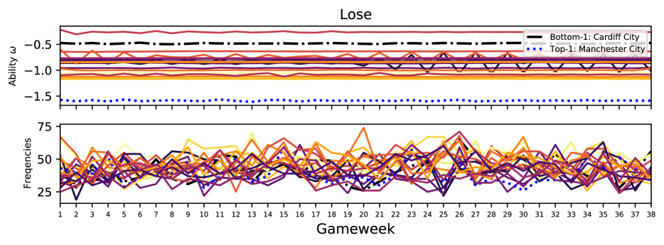
Figure 4: Top panel shows the evolution of losing the possession of the ball (Pass_U) ability $\omega_{c,9}^{(t)}$ for each team across the season. The blue dashed line corresponds to Manchester city, winner of 2013/2014 Premier league while the black dash-dotted line is for the bottom-ranked team Cardiff City. The colors for the rest of the teams have been assigned according to their final rank, with brighter colors associated with teams with a high rank at the end of the championship and darker ones to those having inferior ranks.

Appendix F THE BRANCHING STRUCTURE

We use our proposed model of Section 3.1 to recover event genealogies using its hidden branching structure Hawkes and Oakes (1974). The branching structure categorizes the events into immigrants and offsprings. Offspring events are triggered by previous events while immigrant events are not linked with a parent event. Let $w_{i}^{(s)}$ be the random variable indicating whether the $i$-th event of the $s$-th sequence is an immigrant ($w_{i}^{(s)}=0$) or an offspring ($w_{i}^{(s)}=j$) of a previous event indexed by $j$, we can calculate analytically the conditional branching structure probabilities as

$$p(w_{i}^{(s)}=0|\mathcal{F}_{t_{i}^{(s)}})=\frac{\delta_{u_{i}^{(s)}}^{z_{i}^{(s)}}}{\delta_{u_{i}^{(s)}}^{z_{i}^{(s)}}+\alpha\sum_{k:t_{k}^{(s)}<t_{i}^{(s)}}\gamma_{u_{k}^{(s)},u_{i}^{(s)}}^{z_{i}^{(s)}}\exp\left(-\beta_{u_{k}^{(s)},u_{i}^{(s)}}^{z_{i}^{(s)}}(t_{i}^{(s)}-t_{k}^{(s)})\right)},$$

$$p(w_{i}^{(s)}=j|\mathcal{F}_{t_{i}^{(s)}})=\begin{cases}\frac{\gamma_{u_{j}^{(s)},u_{i}^{(s)}}^{z_{i}^{(s)}}\exp\left(-\beta_{u_{j}^{(s)},u_{i}^{(s)}}^{z_{i}^{(s)}}(t_{i}^{(s)}-t_{j}^{(s)})\right)}{\delta_{u_{i}^{(s)}}^{z_{i}^{(s)}}+\alpha\sum_{k:t_{k}^{(s)}<t_{i}^{(s)}}\gamma_{u_{k}^{(s)},u_{i}^{(s)}}^{z_{i}^{(s)}}\exp\left(-\beta_{u_{k}^{(s)},u_{i}^{(s)}}^{z_{i}^{(s)}}(t_{i}^{(s)}-t_{k}^{(s)})\right)},&\quad\text{if}~{}~{}t_{j}^{(s)}<t_{i}^{(s)}\\ 0,&\quad\text{otherwise.}\\ \end{cases}$$

The above probabilities are based on the model in (11) and their computation allows us to gain insights over the causality of the event occurrences by assuming a causal constraint that any event is triggered by exactly one of the previous events or the background. Hence, this calculation of probabilities attains the recovering of the hidden branching structure $w_{i}^{(s)}$. We choose four different matches of the 2013/14 EPL winner Manchester City (MC) and we build the branching structure taking into account the last ten events before a MC’s player scores the first goal in the first half of the game. More details are given in the caption of Figure 5. To gain better intuition of how this experiment is related to the real matches we provide the links of the videos with the goals scored from these four matches in the supplementary material. For the leftmost panel of Figure 5, we observe that our model suggests the events "A_Clear“ and "H_Dribble“, the first and third event, respectively, before the first goal is scored, are the most probable event that leads to this goal. Interestingly, by watching the corresponding video, we observe that these two events play a crucial role for scoring this goal since MC’s player Silva by dribbling/conveying the ball closer to the opponent’s goal area creates the right circumstances for scoring the goal himself. The event "A_Clear“, which is the most probable event that lead to a goal, is not unexpected since the main reason this goal was scored because a (failed) attempt of the opponent to move the ball away from his goal area. In the rightmost panel, the branching structure suggests that the goal was primarily a result of a player regaining possession of the ball from the opponent, i.e. the event "A_Win“. The event "H_Save“ also contributed to the triggering of the goal event. The video of the goal interestingly verifies that this goal was scored after MC’s player Jesús Navas gained possession of the ball, leading to a fast counter-attack which was the main reason of the goal. The other event is also important since after the opponent’s goalkeeper prevented a goal by the shoot of Edin Džeko, the ball landed at Silva’s feet allowing him to easily score. It is encouraging that our model is able to capture such a level of detail in football dynamics while preserving interpretability.

F.1 Links of videos

The links of the videos for the two matches of Figure 5 accompanied with the right time interval of the goal in the video in parentheses, the date of the match, the name of the MC’s player who scored the first goal, and the final score.

MC vs Newcastle United.

Url: https://www.youtube.com/watch?v=ycnM_V273Zc&ab_channel=HDKoooralive (see 0:00 - 1:00)   Date: 19/08/2013   Scorer’s name of first goal: Silva   Final score: 4-0

Arsenal vs MC.

Url: https://www.youtube.com/watch?v=PQQqlGVb0Lk&ab_channel=mrszippy (see 0:00 - 0:57)   Date: 29/03/2014   Scorer’s name of first goal: Silva   Final score: 1-1

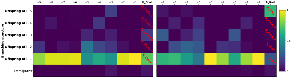
Figure 5: Branching structure of the last 10 events before the first goal scored by Manchester City in the first half of the game from four different matches played by Manchester City (MC). The games are MC vs Newcastle United on 19/08/2013 (leftmost panel) and Arsenal vs MC on 29/03/2014 (rightmost panel). Each plot reads bottom-up with each column representing a probability vector which gives the probability the event on the x-axis is triggered by an immigrant or by an offspring that occurred at most 5 events in advance. The last column always depicts the sequence of the last 5 events (event types in red) before the MC scores. The prefixes ‘H’ or ‘A’ indicates whether MC is the home or away team and the suffixes ‘U’ and ‘S’ indicate whether the passes were unsuccessful or successful, respectively.

References

- Bacry and Muzy (2016) Emmanuel Bacry and Jean-Francois Muzy. First- and second-order statistics characterization of Hawkes processes and non-parametric estimation. IEEE Transactions on Information Theory, 62(4):2184–2202, 2016.
- Bacry et al. (2015) Emmanuel Bacry, Adrian Iuga, Matthieu Lasnier, and Charles-Albert Lehalle. Market impacts and the life cycle of investors orders. Market Microstructure and Liquidity, 1(02):1550009, 2015.
- Bacry et al. (2016) Emmanuel Bacry, Thibault Jaisson, and Jean-François Muzy. Estimation of slowly decreasing hawkes kernels: application to high-frequency order book dynamics. Quantitative Finance, 16(8):1179–1201, 2016.
- Bhattacharjya et al. (2018) Debarun Bhattacharjya, Dharmashankar Subramanian, and Tian Gao. Proximal graphical event models. Advances in Neural Information Processing Systems, 31:8136–8145, 2018.
- Blei et al. (2003) David M Blei, Andrew Y Ng, and Michael I Jordan. Latent Dirichlet allocation. Journal of machine Learning research, 3(Jan):993–1022, 2003.
- Blei et al. (2017) David M Blei, Alp Kucukelbir, and Jon D McAuliffe. Variational inference: A review for statisticians. Journal of the American statistical Association, 112(518):859–877, 2017.
- Bonnet et al. (2021) Anna Bonnet, Miguel Martinez Herrera, and Maxime Sangnier. Maximum likelihood estimation for hawkes processes with self-excitation or inhibition. Statistics & Probability Letters, 179:109214, 2021.
- Bowsher (2007) Clive G Bowsher. Modelling security market events in continuous time: Intensity based, multivariate point process models. Journal of Econometrics, 141(2):876–912, 2007.
- Chen et al. (2017) Shizhe Chen, Ali Shojaie, Eric Shea-Brown, and Daniela Witten. The multivariate hawkes process in high dimensions: Beyond mutual excitation. arXiv preprint arXiv:1707.04928, 2017.
- Clemente et al. (2015) Filipe Manuel Clemente, Fernando Manuel Lourenço Martins, Dimitris Kalamaras, P Del Wong, and Rui Sousa Mendes. General network analysis of national soccer teams in fifa world cup 2014. International Journal of Performance Analysis in Sport, 15(1):80–96, 2015.
- Costa et al. (2020) Manon Costa, Carl Graham, Laurence Marsalle, and Viet Chi Tran. Renewal in hawkes processes with self-excitation and inhibition. Advances in Applied Probability, 52(3):879–915, 2020.
- Cunningham et al. (2007) John P Cunningham, Byron M Yu, Krishna V Shenoy, and Maneesh Sahani. Inferring neural firing rates from spike trains using Gaussian processes. Advances in neural information processing systems, 20:329–336, 2007.
- Decroos et al. (2017) Tom Decroos, Vladimir Dzyuba, Jan Van Haaren, and Jesse Davis. Predicting soccer highlights from spatio-temporal match event streams. In Proceedings of the AAAI Conference on Artificial Intelligence, volume 31, 2017.
- Decroos et al. (2019) Tom Decroos, Lotte Bransen, Jan Van Haaren, and Jesse Davis. Actions speak louder than goals: Valuing player actions in soccer. In Proceedings of the 25th ACM SIGKDD International Conference on Knowledge Discovery & Data Mining, pages 1851–1861, 2019.
- Didelez (2008) Vanessa Didelez. Graphical models for marked point processes based on local independence. Journal of the Royal Statistical Society: Series B (Statistical Methodology), 70(1):245–264, 2008.
- Ding et al. (2018) Hongyi Ding, Mohammad Khan, Issei Sato, and Masashi Sugiyama. Bayesian nonparametric Poisson-process allocation for time-sequence modeling. In International Conference on Artificial Intelligence and Statistics, pages 1108–1116, 2018.
- Donnet et al. (2020) Sophie Donnet, Vincent Rivoirard, Judith Rousseau, et al. Nonparametric bayesian estimation for multivariate hawkes processes. Annals of Statistics, 48(5):2698–2727, 2020.
- Du et al. (2016) Nan Du, Hanjun Dai, Rakshit Trivedi, Utkarsh Upadhyay, Manuel Gomez-Rodriguez, and Le Song. Recurrent marked temporal point processes: Embedding event history to vector. In Proceedings of the 22nd ACM SIGKDD International Conference on Knowledge Discovery and Data Mining, pages 1555–1564, 2016.
- Duane et al. (1987) Simon Duane, Anthony D Kennedy, Brian J Pendleton, and Duncan Roweth. Hybrid Monte Carlo. Physics letters B, 195(2):216–222, 1987.
- Duch et al. (2010) Jordi Duch, Joshua S Waitzman, and Luís A Nunes Amaral. Quantifying the performance of individual players in a team activity. PloS one, 5(6):e10937, 2010.
- Eichler et al. (2017) Michael Eichler, Rainer Dahlhaus, and Johannes Dueck. Graphical modeling for multivariate Hawkes processes with nonparametric link functions. Journal of Time Series Analysis, 38(2):225–242, 2017.
- Gregory and Loredo (1992) PC Gregory and Thomas J Loredo. A new method for the detection of a periodic signal of unknown shape and period. The Astrophysical Journal, 398:146–168, 1992.
- Grund (2012) Thomas U Grund. Network structure and team performance: The case of english premier league soccer teams. Social Networks, 34(4):682–690, 2012.
- Gudmundsson and Horton (2017) Joachim Gudmundsson and Michael Horton. Spatio-temporal analysis of team sports. ACM Computing Surveys (CSUR), 50(2):1–34, 2017.
- Gunawardana et al. (2011) Asela Gunawardana, Christopher Meek, and Puyang Xu. A model for temporal dependencies in event streams. Advances in neural information processing systems, 24:1962–1970, 2011.
- Hansen et al. (2015) Niels Richard Hansen, Patricia Reynaud-Bouret, Vincent Rivoirard, et al. Lasso and probabilistic inequalities for multivariate point processes. Bernoulli, 21(1):83–143, 2015.
- Hawkes (1971) Alan G Hawkes. Spectra of some self-exciting and mutually exciting point processes. Biometrika, 58(1):83–90, 1971.
- Hawkes and Oakes (1974) Alan G Hawkes and David Oakes. A cluster process representation of a self-exciting process. Journal of Applied Probability, pages 493–503, 1974.
- Iwata et al. (2013) Tomoharu Iwata, Amar Shah, and Zoubin Ghahramani. Discovering latent influence in online social activities via shared cascade Poisson processes. In Proceedings of the 19th ACM SIGKDD international conference on Knowledge discovery and data mining, pages 266–274, 2013.
- Jankowiak and Obermeyer (2018) Martin Jankowiak and Fritz Obermeyer. Pathwise derivatives beyond the reparameterization trick. In International Conference on Machine Learning, pages 2235–2244, 2018.
- Johnson et al. (2016) Alistair EW Johnson, Tom J Pollard, Lu Shen, H Lehman Li-Wei, Mengling Feng, Mohammad Ghassemi, Benjamin Moody, Peter Szolovits, Leo Anthony Celi, and Roger G Mark. Mimic-iii, a freely accessible critical care database. Scientific data, 3(1):1–9, 2016.
- Kingma and Ba (2014) Diederik P Kingma and Jimmy Ba. Adam: A method for stochastic optimization. arXiv preprint arXiv:1412.6980, 2014.
- Kingma and Welling (2013) Diederik P Kingma and Max Welling. Auto-encoding variational bayes. arXiv preprint arXiv:1312.6114, 2013.
- Kumar et al. (2019) Srijan Kumar, Xikun Zhang, and Jure Leskovec. Predicting dynamic embedding trajectory in temporal interaction networks. In Proceedings of the 25th ACM SIGKDD International Conference on Knowledge Discovery & Data Mining, pages 1269–1278, 2019.
- Lee et al. (2016) Young Lee, Kar Wai Lim, and Cheng Soon Ong. Hawkes processes with stochastic excitations. In International Conference on Machine Learning, pages 79–88. PMLR, 2016.
- Lemonnier and Vayatis (2014) Remi Lemonnier and Nicolas Vayatis. Nonparametric markovian learning of triggering kernels for mutually exciting and mutually inhibiting multivariate hawkes processes. In Joint European Conference on Machine Learning and Knowledge Discovery in Databases, pages 161–176. Springer, 2014.
- Lewis et al. (2012) Erik Lewis, George Mohler, P Jeffrey Brantingham, and Andrea L Bertozzi. Self-exciting point process models of civilian deaths in iraq. Security Journal, 25(3):244–264, 2012.
- Li et al. (2018) Shuang Li, Shuai Xiao, Shixiang Zhu, Nan Du, Yao Xie, and Le Song. Learning temporal point processes via reinforcement learning. In Proceedings of the 32nd International Conference on Neural Information Processing Systems, pages 10804–10814, 2018.
- Linderman and Adams (2015) Scott W Linderman and Ryan P Adams. Scalable bayesian inference for excitatory point process networks. arXiv preprint arXiv:1507.03228, 2015.
- Lindqvist (2006) Bo Henry Lindqvist. On the statistical modeling and analysis of repairable systems. Statistical science, 21(4):532–551, 2006.
- Liu and Hauskrecht (2019) Siqi Liu and Milos Hauskrecht. Nonparametric regressive point processes based on conditional Gaussian processes. In Advances in Neural Information Processing Systems, pages 1064–1074, 2019.
- Lloyd et al. (2016) Chris Lloyd, Tom Gunter, Michael Osborne, Stephen Roberts, and Tom Nickson. Latent point process allocation. In Artificial Intelligence and Statistics, pages 389–397, 2016.
- Marsan and Lengline (2008) David Marsan and Olivier Lengline. Extending earthquakes’ reach through cascading. Science, 319(5866):1076–1079, 2008.
- Mei and Eisner (2017) Hongyuan Mei and Jason M Eisner. The neural Hawkes process: A neurally self-modulating multivariate point process. In Advances in Neural Information Processing Systems, pages 6754–6764, 2017.
- Mohler et al. (2011) George O Mohler, Martin B Short, P Jeffrey Brantingham, Frederic Paik Schoenberg, and George E Tita. Self-exciting point process modeling of crime. Journal of the American Statistical Association, 106(493):100–108, 2011.
- Narayanan (2020) Santhosh Narayanan. Bayesian modelling of marked spatio-temporal point processes with applications to event sequences from association football. PhD thesis, Department of Statistics, University of Warwick, 2020. Available at http://wrap.warwick.ac.uk/153205/.
- Narayanan et al. (2021) Santhosh Narayanan, Ioannis Kosmidis, and Petros Dellaportas. Flexible marked spatio-temporal point processes with applications to event sequences from association football. arXiv preprint arXiv:2103.04647 (accepted for a Discussion Paper in the Journal of the Royal Statistical Society: Series C), 2021.
- Ogata (1981) Yosihiko Ogata. On Lewis’ simulation method for point processes. IEEE transactions on information theory, 27(1):23–31, 1981.
- Ogata (1998) Yosihiko Ogata. Space-time point-process models for earthquake occurrences. Annals of the Institute of Statistical Mathematics, 50(2):379–402, 1998.
- Okawa et al. (2019) Maya Okawa, Tomoharu Iwata, Takeshi Kurashima, Yusuke Tanaka, Hiroyuki Toda, and Naonori Ueda. Deep mixture point processes: Spatio-temporal event prediction with rich contextual information. In Proceedings of the 25th ACM SIGKDD International Conference on Knowledge Discovery & Data Mining, pages 373–383, 2019.
- Passos et al. (2011) Pedro Passos, Keith Davids, Duarte Araújo, N Paz, J Minguéns, and Jose Mendes. Networks as a novel tool for studying team ball sports as complex social systems. Journal of Science and Medicine in Sport, 14(2):170–176, 2011.
- Paszke et al. (2019) Adam Paszke, Sam Gross, Francisco Massa, Adam Lerer, James Bradbury, Gregory Chanan, Trevor Killeen, Zeming Lin, Natalia Gimelshein, Luca Antiga, et al. Pytorch: An imperative style, high-performance deep learning library. Advances in Neural Information Processing Systems, 32:8026–8037, 2019.
- Ranganath et al. (2014) Rajesh Ranganath, Sean Gerrish, and David Blei. Black box variational inference. In Artificial intelligence and statistics, pages 814–822. PMLR, 2014.
- Rasmussen and Williams (2006) Carl Edward Rasmussen and Christopher K. I. Williams. Gaussian processes for machine learning, volume 2. MIT press Cambridge, MA, 2006.
- Reinhart et al. (2018) Alex Reinhart et al. A review of self-exciting spatio-temporal point processes and their applications. Statistical Science, 33(3):299–318, 2018.
- Robberechts et al. (2019) Pieter Robberechts, Jan Van Haaren, and Jesse Davis. Who will win it? an in-game win probability model for football. arXiv preprint arXiv:1906.05029, 2019.
- Routley and Schulte (2015) Kurt Routley and Oliver Schulte. A Markov game model for valuing player actions in ice hockey. In Conference on Uncertainty in Artificial Intelligence (UAI), pages 782–791, 2015.
- Rue and Held (2005) Havard Rue and Leonhard Held. Gaussian Markov random fields: theory and applications. CRC press, 2005.
- Salehi et al. (2019) Farnood Salehi, William Trouleau, Matthias Grossglauser, and Patrick Thiran. Learning Hawkes processes from a handful of events. In Advances in Neural Information Processing Systems, pages 12715–12725, 2019.
- Shchur et al. (2019) Oleksandr Shchur, Marin Biloš, and Stephan Günnemann. Intensity-free learning of temporal point processes. In International Conference on Learning Representations, 2019.
- Van Haaren et al. (2016) Jan Van Haaren, Siebe Hannosset, and Jesse Davis. Strategy discovery in professional soccer match data. In Proceedings of the KDD-16 Workshop on Large-Scale Sports Analytics, pages 1–4, 2016.
- Vaswani et al. (2017) Ashish Vaswani, Noam Shazeer, Niki Parmar, Jakob Uszkoreit, Llion Jones, Aidan N Gomez, Lukasz Kaiser, and Illia Polosukhin. Attention is all you need. In NIPS, 2017.
- Wang et al. (2015) Qing Wang, Hengshu Zhu, Wei Hu, Zhiyong Shen, and Yuan Yao. Discerning tactical patterns for professional soccer teams: an enhanced topic model with applications. In Proceedings of the 21th ACM SIGKDD International Conference on Knowledge Discovery and Data Mining, pages 2197–2206, 2015.
- Wang et al. (2016) Yichen Wang, Bo Xie, Nan Du, and Le Song. Isotonic hawkes processes. In International conference on machine learning, pages 2226–2234. PMLR, 2016.
- Xiao et al. (2017) Shuai Xiao, Mehrdad Farajtabar, Xiaojing Ye, Junchi Yan, Xiaokang Yang, Le Song, and Hongyuan Zha. Wasserstein learning of deep generative point process models. In Advances in Neural Information Processing Systems 30, 2017.
- Xu et al. (2016) Hongteng Xu, Mehrdad Farajtabar, and Hongyuan Zha. Learning Granger causality for Hawkes processes. In International conference on machine learning, pages 1717–1726, 2016.
- Yuan et al. (2019) Baichuan Yuan, Hao Li, Andrea L Bertozzi, P Jeffrey Brantingham, and Mason A Porter. Multivariate spatiotemporal hawkes processes and network reconstruction. SIAM Journal on Mathematics of Data Science, 1(2):356–382, 2019.
- Zhang et al. (2018) Cheng Zhang, Judith Bütepage, Hedvig Kjellström, and Stephan Mandt. Advances in variational inference. IEEE transactions on pattern analysis and machine intelligence, 41(8):2008–2026, 2018.
- Zhang et al. (2020a) Qiang Zhang, Aldo Lipani, Omer Kirnap, and Emine Yilmaz. Self-attentive Hawkes process. In International Conference on Machine Learning, pages 11183–11193. PMLR, 2020a.
- Zhang et al. (2020b) Rui Zhang, Christian Walder, and Marian-Andrei Rizoiu. Variational inference for sparse Gaussian process modulated hawkes process. In Proceedings of the AAAI Conference on Artificial Intelligence, volume 34, pages 6803–6810, 2020b.
- Zhao et al. (2015) Qingyuan Zhao, Murat A Erdogdu, Hera Y He, Anand Rajaraman, and Jure Leskovec. Seismic: A self-exciting point process model for predicting tweet popularity. In Proceedings of the 21th ACM SIGKDD international conference on knowledge discovery and data mining, pages 1513–1522, 2015.
- Zhou et al. (2013) Ke Zhou, Hongyuan Zha, and Le Song. Learning triggering kernels for multi-dimensional Hawkes processes. In International Conference on Machine Learning, pages 1301–1309, 2013.
- Zuo et al. (2020) Simiao Zuo, Haoming Jiang, Zichong Li, Tuo Zhao, and Hongyuan Zha. Transformer Hawkes process. In International conference on machine learning, pages 11692–11702. PMLR, 2020.