Chemical complexity of phosphorous bearing species in various regions of the Interstellar medium

Abstract

Phosphorus related species are not known to be as omnipresent in space as hydrogen, carbon, nitrogen, oxygen, and sulfur-bearing species. Astronomers spotted very few P-bearing molecules in the interstellar medium and circumstellar envelopes. Limited discovery of the P-bearing species imposes severe constraints in modeling the P-chemistry. In this paper, we carry out extensive chemical models to follow the fate of P-bearing species in diffuse clouds, photon-dominated or photodissociation regions (PDRs), and hot cores/corinos. We notice a curious correlation between the abundances of PO and PN and atomic nitrogen. Since N atoms are comparatively abundant in diffuse clouds and PDRs than in the hot core/corino region, PO/PN reflects $<1$ in diffuse clouds, $<<1$ in PDRs, and $>1$ in the late warm-up evolutionary phase of the hot core/corino regions. During the end of the post-warm-up phase, we obtain PO/PN $>1$ for hot core and $<1$ for its low mass analog. We employ a radiative transfer model to investigate the transitions of some of the P-bearing species in diffuse cloud and hot core regions and estimate the line profiles. Our study estimates the required integration time to observe these transitions with ground-based and space-based telescopes. We also carry out quantum chemical computation of the infrared features of PH₃ along with various impurities. We notice that SO₂ overlaps with the PH₃ bending-scissoring modes around $\sim(1000-1100)$ cm^-1. We also find that the presence of CO₂ can strongly influence the intensity of the stretching modes around $\sim 2400$ cm^-1 of PH₃.

1 Introduction

Phosphorus (P) and its compounds play a crucial role in the chemical evolution in galaxies. Phosphorus is an essential element of life and is one of the main biogenic elements. Its origin in the terrestrial system is yet to be fully understood. The Atacama Large Millimeter/submillimeter Array (ALMA) and European Space Agency Probe Rosetta suggest that P-related species might have traveled from star-forming regions to the Earth (e.g. Altwegg et al., 2016; Rivilla et al., 2020) through comets. The interstellar chemistry of P-bearing molecules has significant astrophysical relevance, and very little has been revealed so far. P-bearing compounds are the major components of any living system, where they carry out numerous biochemical functions. P-bearing molecules play a significant role in forming large bio-molecules or living organisms; they store and transmit the genetic information in nucleic acids and work in nucleotides as precursors in the synthesis of RNA and DNA (Maciá et al., 1997). Moreover, these molecules are the essential components of phospholipids (main characteristic features of cellular membranes, Maciá, 2005).

Phosphorus is relatively rare in the interstellar medium (ISM). However, it is ubiquitous in various meteorites (Jarosewich, 1990; Pasek, 2019; Lodders, 2003). On average, P is the thirteenth most abundant element in a typical meteoritic material and the eleventh most abundant element in the Earth’s crust (Maciá, 2005).

Jura & York (1978) identified P⁺ with a cosmic abundance of $\sim 2\times 10^{-7}$ in hot regions ($\sim 1200$ K). P-bearing molecules such as PN, PO, HCP, CP, CCP, PH₃ have been observed in circumstellar envelopes around evolved stars (Guelin et al., 1990; Tenenbaum et al., 2007; Agúndez et al., 2007, 2008; Tenenbaum & Ziurys, 2008; Halfen et al., 2008; Milam et al., 2008; De Beck et al., 2013; Agúndez et al., 2014; Ziurys et al., 2018). PN was detected in several star-forming regions (Turner & Bally, 1987; Ziurys, 1987; Turner et al., 1990; Caux et al., 2011; Yamaguchi et al., 2011; Fontani et al., 2016; Mininni et al., 2018; Fontani et al., 2019), and it remained the only P-containing species identified in dense ISM for many years (Ziurys, 1987; Turner et al., 1990; Fontani et al., 2016). Rivilla et al. (2016) reported the first detection of PO toward two massive star-forming regions W51 1e/2e and W3(OH), along with PN by using the IRAM 30m telescope. Thereafter, both PO and PN were simultaneously observed in several low and high mass star-forming regions and Galactic Centre (Lefloch et al., 2016; Rivilla et al., 2018, 2020; Bergner et al., 2019; Bernal et al., 2021).

Theoretical investigation on P-chemistry modeling has been extensively reported in several studies (Millar, 1991; Charnley & Millar, 1994; Aota & Aikawa, 2012; Lefloch et al., 2016; Rivilla et al., 2016; Jiménez-Serra et al., 2018). However, the P-chemistry of the dense cloud region is not well constrained. The main uncertainty lies in the depletion factor of the initial elemental abundance of P. The degree of complexity of gas-phase abundance within the gas and the exact depletion of different elements onto the grains are still uncertain (Jenkins, 2009). Very recently, Nguyen et al. (2020) discovered the chemical desorption of phosphine. This kind of study is indeed very crucial in constraining the modeling parameters.

Phosphine (PH₃) is the phosphorus cousin of ammonia (NH₃) and is a relatively stable molecule that could hold a significant fraction of P in various astronomical environments. Scientists consider PH₃ to be a biosignature (Sousa-Silva et al., 2020). PH₃ was identified in the planets of our solar system containing a reducing atmosphere. The Voyager data confirmed PH₃ within Jupiter and Saturn with volume mixing ratios of 0.6 and 2 ppm, respectively (Maciá, 2005). It further suggested that the P/H ratio shows harmony with the solar value. Fletcher et al. (2009) derived the global distribution of PH₃ on Jupiter and Saturn using 2.5 cm^-1 spectral resolution of Cassini/CIRS observations. PH₃ could be produced deep inside the reducing atmospheres of giant planets (Bregman et al., 1975; Tarrago et al., 1992) at high temperatures and pressures, and dredged upwards by the convection (Noll & Marley, 1997; Visscher et al., 2006). Very surprisingly, in Venus, there is no such reducing atmosphere, but $\sim 20$ ppb of PH₃ was inferred (Greaves et al., 2020) in the deck of venus atmosphere. They could not account for such a high amount of PH₃ with the steady-state chemical models, including the photochemical pathways. They also explored the other abiotic routes for explaining this high abundance. But none of them seems to be suitable. They speculated some unknown photo or geo-chemical origin of it. More far-reaching, its high abundance by some of the biological means could not be ruled out. Bains et al. (2020) also could not explain the presence of PH₃ in Venus’s clouds by any abiotic mechanism based on their state-of-the-art understanding. This discovery opened up a series of debates. Very recently, Villanueva et al. (2020) question about the analysis and interpretation of the spectroscopic data used in Greaves et al. (2020). These authors claimed that there is no PH₃ in Venus’s atmosphere. Snellen et al. (2020) also found no statistical evidence for PH₃ in the atmosphere of Venus.

Among the simple P-bearing species, PH₃ was tentatively identified (J = 1 $\rightarrow$ 0, $266.9$ GHz) in the envelope of the carbon-rich stars IRC +10216 and CRL 2688 (Tenenbaum & Ziurys, 2008; Agúndez et al., 2008). Later, the presence of PH₃ was confirmed by Agúndez et al. (2014). They observed the J = 2 $\rightarrow$ 1 rotational transition of PH₃ (at $534$ GHz) in IRC +10216 using the HIFI instrument on board Herschel. They predicted a very high abundance of PH₃ in this region. Suppose the gas-phase reactions are responsible for such a high abundance of PH₃. In that case, it should occur through a barrierless reaction or with a reaction with a little barrier at low temperatures. Here, we employ various state-of-the-art chemical models to understand the formation of PH₃ under different interstellar conditions like diffuse cloud, interstellar photon dominated regions or photodissociation regions (PDRs), and hot core regions.

Recently, Chantzos et al. (2020) attempted to observe HCP (2–1), CP (2–1), PN (2–1), and PO (2–1) with the IRAM 30m telescope along the line of sight to the compact extra-galactic quasar B0355+508. They were unable to detect these transitions along this line of sight. But based on their observations, they predicted 3$\sigma$ upper limits of these transitions. However, they successfully identified HNC (1–0), CN (1–0), and C³⁴S (2–1) in absorption and ¹³CO (1–0) in emission along the same line of sight.

We organize this paper as follows. In Section 2, we prepare a currently available chemical network for the P-bearing species, and in Section 3, we present their various kinetic information. Section 4 is devoted to the chemical model explaining P-chemistry in different parts of the ISM. In Section 5, we describe our results obtained with the radiative transfer model for the diffuse and hot core region. In Section 6, we explain the infrared spectrum of PH₃ ice under various circumstances, and finally, in Section 7, we draw our conclusion.

2 The chemical network of phosphorus

We prepare an extensive network to study the chemistry of the P-bearing species. Since nitrogen (N) and P have five electrons in the valance shell, P-chemistry is sometimes considered analogous to N-chemistry. For example, successive hydrogenation of N yields NH₃, whereas, for P, it yields PH₃. However, the presence of NH₃ is ubiquitous in the ISM (Cheung et al., 1968; Wilson & Pauls, 1979; Keene et al., 1983; Mauersberger et al., 1988), the presence of PH₃ is not so universal (Thorne et al., 1983). On the other hand, P’s chemistry can notably differ from the N-related chemistry under the physical conditions prevailing in the different star-forming regions. In this paper, we prepare an extensive network of P by following the chemical pathways explained in Thorne et al. (1984); Adams et al. (1990); Millar (1991); Fontani et al. (2016); Jiménez-Serra et al. (2018); Sousa-Silva et al. (2020); Rivilla et al. (2016); Chantzos et al. (2020). Charnley & Millar (1994) and Anicich (1993) differentiated the formation/destruction mechanism of PH_n (n=1, 2, 3) and their cationic species. Thorne et al. (1984) presented the reaction pathways for P, PO, P⁺, PO⁺, PH⁺, HPO⁺ and H₂PO⁺. Furthermore, in a recent study, Chantzos et al. (2020) extends the gas-phase chemical network of PN and PO in accordance with Millar et al. (1987) & Jiménez-Serra et al. (2018). We use the kinetic data of chemical reactions from the KInetic Database for Astrochemistry (Wakelam et al., 2015) (hereafter, KIDA) and the UMIST Database for Astrochemistry (UDfA, McElroy et al., 2013). In the Appendix Table 10, we show all the reactions considered in our P-network.

Table 1: Calculated binding energy (with MP2/aug-cc-pVDZ) and enthalpy of formation (with DFT-B3LYP/6-31G(d,p)) of P-bearing species.

Serial	Species	Astronomical	Ground	Binding Energy [Kelvin]						Enthalpy of formation [kJ/mol]
No.		status	state	CO monomer	CH3OH monomer	H2O monomer	H2O tetramer	H2 monomer	Availabled	Our calculated	Availabled
1.	P	$\cdots$	quartet	170	442	270	616c	107	1100	315.557a, 310.202b	315.663a, 316.5b
2.	P2	not observed	singlet	378	904	494	1671	223	$\cdots$	182.260a, 180.434b	145.8a
3.	PN	observed	singlet	324	2560	2326	2838	399	1900	218.985a, 217.974b	172.48a, 171.487b
4.	PO	observed	doublet	703	4334	2818	4600	508	1900	13.483a, 12.490b	-27.548a, -27.344b
5.	HCP	observed	singlet	572	2122	1723	2468	132	2350	251.466a, 250.054b	217.79a, 216.363b
6.	CP	observed	doublet	300	1335	1126	1699c	165	1900	538.388a, 540.696b	517.86a, 520.162b
7.	CCP	observed	doublet	2181	3900	2701	2868	396	4300	660.424a, 664.413b	$\cdots$
8.	HPO	not observed	singlet	602	4097	2838	5434	521	2350	-38.035a, -41.915b	-89.9a, -93.7b
9.	PH	not observed	triplet	270	780	491	944c	134	1550	228.785a, 227.878b	231.698a, 230.752b
10.	PH2	not observed	doublet	285	851	965	1226c	138	2000	128.872a, 125.036b	139.333a, 135.474b
11.	PH3	observed	singlet	716	952	606	1672	545	$\cdots$	12.934a, 5.006b	13.4a

Note. — ^aEnthalpy of formation at T = 0 K and 1 atmosphere pressure, ^bEnthalpy of formation at T = 298 K and 1 atmosphere pressure, ^cDas et al. (2018), ^dKIDA (http://kida.astrophy.u-bordeaux.fr)

3 The binding energy of P-bearing species

A continuous exchange of chemical ingredients within the gas and grain can determine the chemical complexity of the ISM. The major drawback in constraining this chemical process by astrochemical modeling is the lack of information about the interaction energy of the chemical species with the grain surface. The fate of the chemical complexity on the grain surface depends on the residence time of the incoming species on the grain. Thus, the binding energy (BE) of interstellar species plays a crucial role in the chemical complexity of the ISM.

In a periodic treatment of surface adsorption phenomena, BE is related to the interaction energy ($\Delta$E), as:

$$BE=-\Delta E$$ (1)

For a bounded adsorbate BE is a positive quantity and is defined as:

$$BE=(E_{surface}+E_{species})-E_{ss}$$ (2)

where $\rm{E_{ss}}$ is the optimized energy for the complex system where a species is placed at a distance from the grain surface through a weak Van der Waals interaction. $\rm{E_{surface}}$ and $\rm{E_{species}}$ are the optimized energies of the grain surface and species, respectively.

In dense molecular clouds, a sizeable portion of the grain mantle would cover water, methanol, and CO molecules. In more dense regions, gas-phase H₂ could easily accrete on the grain and mostly gets back to the gas phase due to their low sticking probability and lower BEs. But some H₂ could be trapped under some accreting species. For example, one H₂ may accrete on another H₂ before it is desorbed. In this situation, the “encounter desorption” mechanism is supposed to be an essential means of transportation of H₂ to the gas phase (Hincelin et al., 2015). Usually, in the literature, only the encounter desorption of H₂ is considered due to its wide presence in the dense interstellar medium. Recently, Chang et al. (2021) considered the encounter desorption of H atom as well. But the BEs of the interstellar species with the different substrates are unknown. Looking at these aspects, in Table 1, we report the BEs of some relevant P-bearing species by considering H₂O, CO, CH₃OH, and H₂ as a substrate. The computed BEs should have a range of values that depend on the molecule’s position on the ice (Das et al., 2018; Ferrero et al., 2020). Whenever we have obtained different BE values at other binding sites, we exert the average of some of our calculations and note in Table 1. In this paper, we only consider the BE with water substrate for our simulation. BEs with the other substrates are provided for future usage. We perform all the BE calculations by Gaussian 09 suite of programs (Frisch et al., 2013) using Equations 1 and 2. To find the optimized energy of all structures, we use a Second-order Møller-Plesset (MP2) method with an aug-cc-pVDZ basis set (Dunning, 1989). We did not include the zero-point vibrational energy (ZPVE) and basis set superposition error (BSSE) correction (Das et al., 2018). A fully optimized ground-state structure is verified to be a stationary point (having non-imaginary frequency) by harmonic vibrational frequency analysis. Ground state spin multiplicity of the species is also noted in Table 1. To evaluate it, we take the help of the Gaussian 09 suite of programs and run separate calculations (job type “opt+freq”), each with different spin multiplicities, and then compare the results between them. The lowest energy electronic state solution of the chosen spin multiplicity is the ground state noted.

Due to the similarities between the structure of NH₃ and PH₃, Chantzos et al. (2020) considered the BE of PH₃ same as NH₃. The BE of NH₃ is $5800$ K according to the KIDA database. Since they also used this BE of PH₃, they did not obtain much PH₃ by thermal desorption process in the cold regions. They pointed out that most of the PH₃ came to the gas phase by photo-desorption rather than thermal desorption from the colder region. In our calculation, we found a noticeable decrease in the BE of PH₃, which could enable PH₃ to populate the gas phase by thermal desorption even at low temperatures. Das et al. (2018) noted BE of NH₃ with a c-hexamer configuration of water $\sim 5163$ K, whereas we have found it $\sim 2395$ K for PH₃. With significant ice constituents (monomer of CO, CH₃OH, H₂O, and H₂), our computed BE of PH₃ seems to be $<1000$ K. Sousa-Silva et al. (2020) noted that PH₃ has very low water solubility (at 17 ^∘C only 22.8 ml of gaseous PH₃ dissolve in 100 ml of water), and it does not easily stick to aerosols. The recent claim of PH₃ in the Venusian atmosphere (Greaves et al., 2020) prompted us to determine the BE of PH₃ with some other species like sulfuric acid (H₂SO₄) and Benzene ($\rm{C_{6}H_{6}}$). $\rm{H_{2}SO_{4}}$ which are the principal constituents of the Venus atmosphere. Our computed BE with $\rm{H_{2}SO_{4}}$ and Benzene is $\sim 2271$ K and $\sim 3094$ K, respectively. However, Snellen et al. (2020) and Villanueva et al. (2020) questioned about the identification of Greaves et al. (2020). Table 1 also provides our calculated enthalpy of formation for several P-bearing species and the BE values noted in various places.

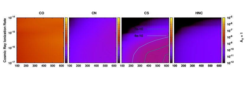
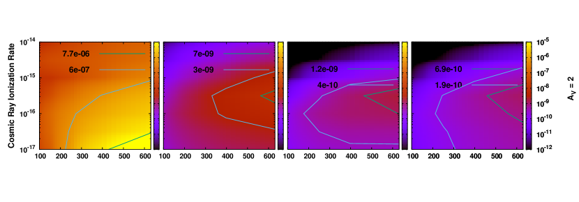
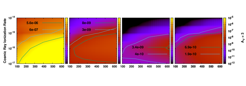
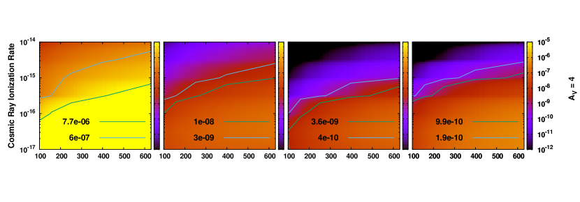
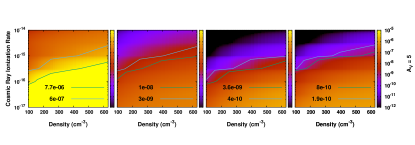
Figure 1: Parameter space of the abundances of CO, CN, CS, and HNC for $\rm{A_{V}}=1,\ 2,\ 3,\ 4,\ 5$ mag for the diffuse cloud model with the Cloudy code. The right side of each panel is marked with color coded values of abundance with respect to total hydrogen nuclei. The contours are highlighted around the previously observed abundance limit (Chantzos et al., 2020) toward the cloud with $v_{LSR}=-17$ km s^-1, including the inferred uncertainties.

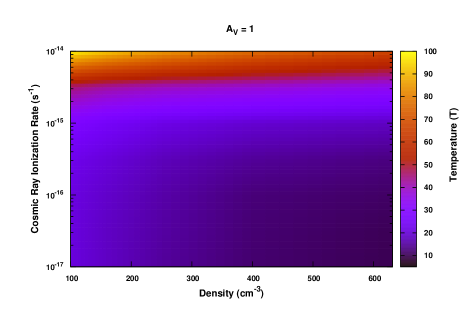
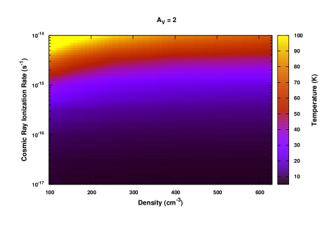
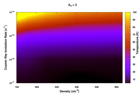
Figure 2: Parameter space of the temperature for $\rm{A_{V}}=1,\ 2,\ 3$ mag for the diffuse cloud model with the Cloudy code. The right side of each panel is marked with color coded values of temperature.

4 chemical model

We use the reaction pathways shown in the Appendix (see Table 10) to check the fate of the P-bearing species in various parts of the ISM (diffuse clouds, PDRs, hot corino, and hot cores). Here, we employ mainly two models to study the chemical evolution of these species; a) spectral synthesis code, Cloudy (version 17.02, last described by Ferland et al., 2017) and b) Chemical Model for Molecular Cloud (hereafter CMMC) code (Das et al., 2015; Gorai et al., 2017a, b; Sil et al., 2018; Gorai et al., 2020; Shimonishi et al., 2020).

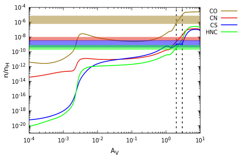
Figure 3: Chemical evolution of the abundances of CO, CN, CS, and HNC for the diffuse cloud model ($\rm{n_{H}}=300$ cm^-3 and $\rm{\zeta=1.7\times 10^{-16}\ s^{-1}}$) with the Cloudy code. The colored horizontal bands correspond to the observed abundances (Chantzos et al., 2020) toward the cloud with $v_{LSR}=-17$ km s^-1, including the inferred uncertainties. The vertical dashed line indicates the visual extinction parameter of best agreement between observation and model results.

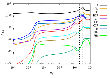
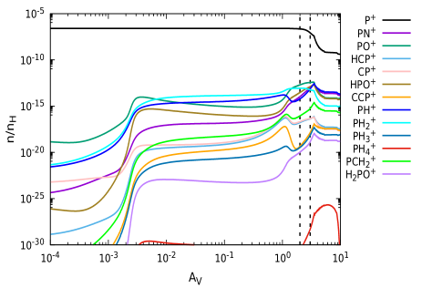
Figure 4: Chemical evolution of the abundances of neutral P-bearing species (left panel), and their corresponding cations (right panel) for the diffuse cloud model ($\rm{n_{H}}=300$ cm^-3 and $\rm{\zeta=1.7\times 10^{-16}\ s^{-1}}$) with the Cloudy code. The vertical dashed line indicates the visual extinction parameter of the best agreement between observation and model results.

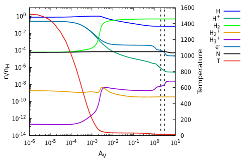
Figure 5: Abundance profiles of H, H⁺, H₂, H${}_{2}^{+}$, H${}_{3}^{+}$, e^-, N, and temperature profile for the diffuse cloud model ($\rm{n_{H}}=300$ cm^-3 and $\rm{\zeta=1.7\times 10^{-16}\ s^{-1}}$) with the Cloudy code. The vertical dashed line indicates the visual extinction parameter of best agreement between observation and model results.

4.1 Spectral synthesis code

We use a photo-ionization code, Cloudy, which simulates matter under a broad range of interstellar conditions. It is for general use under an open-source license. Using Cloudy code, we check the fate of P-bearing species in diffuse cloud and PDR environment.

4.1.1 Diffuse cloud model

Based on the observations carried out by Chantzos et al. (2020), they prepared a diffuse cloud model to explain the observed abundance of HNC, CN, CS, and CO. We also employ a similar process to explain the observed abundances of the four molecules and then look at the fate of the P-bearing molecules under these circumstances. For this modeling, we consider the initial elemental abundance as given in Chantzos et al. (2020). But in Cloudy, only the atomic elemental abundance is allowed (no ionic or molecular form), so we use these abundances as the initial elemental abundance (see Table 2). For each calculation, we check whether the micro-physics considered is time steady or not. We notice that the largest reaction time scale is much shorter than the diffuse cloud’s typical lifetime, $\sim 10^{7}$ years. We use the grain size distribution, which is appropriate for the $R_{V}=3.1$ extinction curve of Mathis et al. (1977). This grain size distribution is called “ISM” in the Cloudy. We use the anisotropic radiation field, which is appropriate for the ISM to specify the intensity of the incident local interstellar radiation field. Additionally, we include the cosmic ray microwave background with a redshift value of $1.52$ (Wenger et al., 2000).

Table 2: Initial elemental abundance for the diffuse cloud and PDR model considered in the Cloudy code.

Element	Abundance	Element	Abundance
H	1.0	Si	$3.2\times 10^{-5}$
He	$8.5\times 10^{-2}$	Fe	$3.2\times 10^{-5}$
N	$6.8\times 10^{-5}$	Na	$1.7\times 10^{-6}$
O	$4.9\times 10^{-4}$	Mg	$3.9\times 10^{-5}$
C	$2.7\times 10^{-4}$	Cl	$3.2\times 10^{-7}$
S	$1.3\times 10^{-5}$	P	$2.6\times 10^{-7}$
		F	$3.6\times 10^{-8}$

Table 3: Estimated column density and optical depth of the observed molecules for the diffuse cloud model with the Cloudy code.

Species	Transitions	Eup [K]	Frequency [GHz]	Optical Depth [$\tau$]		Total Column Density [cm-2]
				Model	Observationa	Model	Observationa
CN	$N=1-0,\ J=1/2-1/2,\ F=3/2-1/2$	5.5	113.16867	0.256522	$0.23\pm 0.07$	$1.47\times 10^{12}$	$(0.87\pm 0.28)\times 10^{13}$
HNC	$J=1-0$	4.4	90.66357	0.33962	$0.50\pm 0.10$	$2.11\times 10^{11}$	$(0.69\pm 0.16)\times 10^{12}$
C34S	$J=2-1$	6.9	96.41295	$\cdots$	$0.04\pm 0.02$	$\cdots$	$(1.64\pm 0.82)\times 10^{11}$
13CO	$J=1-0$	5.3	110.20135	$\cdots$	$0.154\pm 0.004$	$\cdots$	$(3.98\pm 0.16)\times 10^{14}$
HCP	$J=2-1$	5.8	79.90329	$2.56\times 10^{-6}$	$<0.02$	$1.10\times 10^{8}$	$<2.27\times 10^{12}$
PN	$J=2-1$	6.8	93.97977	0.238015	$<0.02$	$1.62\times 10^{11}$	$<4.20\times 10^{10}$
CP	$N=2-1,\ J=3/2-1/2,\ F=2-1$	6.8	95.16416	$4.92\times 10^{-4}$	$<0.02$	$1.16\times 10^{10}$	$<1.26\times 10^{12}$
PO	$J=5/2-3/2,\ \Omega=1/2,\ F=3-2,\ e$	8.4	108.99845	0.0138432	$<0.02$	$9.08\times 10^{10}$	$<4.29\times 10^{11}$
PO	$J=5/2-3/2,\ \Omega=1/2,\ F=2-1,\ e$	8.4	109.04540	0.0125113	$<0.02$	$9.08\times 10^{10}$	$<6.70\times 10^{11}$
PO	$J=5/2-3/2,\ \Omega=1/2,\ F=3-2,\ f$	8.4	109.20620	0.0055508	$<0.02$	$9.08\times 10^{10}$	$<4.34\times 10^{11}$
PO	$J=5/2-3/2,\ \Omega=1/2,\ F=2-1,\ f$	8.4	109.28119	0.0182699	$<0.02$	$9.08\times 10^{10}$	$<6.69\times 10^{11}$

Note. — ^aChantzos et al. (2020)

To check the validity of our model against the observed abundances, we first explain the observed abundance of CO, CN, CS, and HNC as obtained in Chantzos et al. (2020). For this, we use a parameter space for the formation of these species. Our parameter space consists of a density variation of $100-600$ cm^-3 and a cosmic ray ionization rate of H₂ ($\zeta_{H_{2}}$) in between $10^{-17}-10^{-14}$ s^-1. We use a stopping criterion at different $A_{V}$ values. The cases obtained by using stopping criterion $A_{V}=1-5$ mag are given in Figure 1. The observed abundances of CO, CN, CS, and HNC of Chantzos et al. (2020) toward the cloud having a $V_{LSR}=-17$ km s^-1 are highlighted by the contours. Figure 2 shows the variation of temperature at the end of the calculation for $A_{V}=1-3$ mag. The parameter space also consists of the variation of n_H and $\zeta_{H_{2}}$. Temperature variation is shown with the color bar.

From Figure 1 and 2, we see that the parameters which were adopted by Chantzos et al. (2020) for the diffuse cloud model (i.e., $\zeta_{H_{2}}=1.7\times 10^{-16}\ s^{-1}$, $n_{H}=300$ cm^-3 and $T_{gas}=40$ K) can also reproduce the observed abundances of CO, CN, CS, and HNC with our model. Figure 3 shows the obtained abundances of the four molecules when we consider $n_{H}=300$ cm^-3 and $\zeta_{H_{2}}$ = $1.7\times 10^{-16}\ s^{-1}$. The X-axis shows the visual extinction of the cloud, and the Y-axis shows the abundance of n_H. Our results are in agreement with the observation between $A_{V}=2-3$ mag. We highlight the best-suited zone by the black dashed curve. Thus, based on Figures 1, 2, and 3, we use, $A_{V}=2$ mag, $\zeta_{H_{2}}=1.7\times 10^{-16}$, and $n_{H}=300$ cm^-3 as the best fitted parameters to explain the observed abundances of these species. This yields a $A_{V}/N(H)=5.398\times 10^{-22}$ mag cm² and dust to gas ratio of $6.594\times 10^{-3}$. Table 3 compares our obtained optical depth and column densities with the observations. Obtained optical depths of CN and HNC are close to the observed values, but the column densities diverge by a few factors. This slight mismatch is because the Cloudy model deals with steady-state values, but the column densities are time-dependent in reality.

Figure 4 depicts the abundances of most of the P-bearing species considered in this study. The left panel shows the neutral P-bearing species, whereas the right panel shows the P-bearing ions. It is interesting to note that though we consider a neutral atomic abundance in our model, the abundance of P⁺ is high due to the strong cosmic ray ionization and presence of a non-extinguished interstellar radiation field. The abundances of the comparatively larger P-bearing species are very low in the diffuse environment, and it would be pretty challenging to observe them. We notice that some simple neutral P-bearing species like PN, PO, HCP, CP, and PH are significantly more abundant than PH₃. The abundances of PO and PN appear to be comparable to each other (with PO/PN $<1$ when A${}_{V}\geq$ 2). Table 3 shows that the obtained column densities for this case are listed. There is an excellent agreement between the observed and the modeled optical depths of CN and HNC with the Cloudy code.

In Figure 5, the abundances of H, H₂, and N are shown along with the major hydrogen-related ions, H⁺, ${\rm H_{2}}^{+}$, ${\rm H_{3}}^{+}$. In Cloudy, the cloud temperature is calculated self-consistently, depending on the known excitations. The primary source of such excitation is cosmic ray ionization. Figure 5 depicts the gas temperature variation with $A_{V}$ with the solid red curve. Deep inside the cloud, the temperature drops sufficiently and enhances the formation of molecular hydrogen.  For $A_{V}=2$ mag, we obtained a temperature $\sim 10$ K when we use a cosmic ray ionization rate of $1.7\times 10^{-16}$ s^-1. It is a little lower than that used in Chantzos et al. (2020).

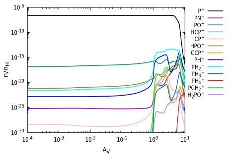
Figure 6: Chemical evolution of the abundances of important P-bearing species with the Cloudy code considering Röllig et al. (2007) F4 PDR model.

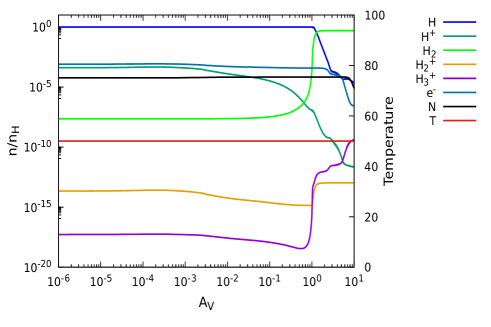
Figure 7: Abundance profiles of H, H⁺, H₂, H${}_{2}^{+}$, H${}_{3}^{+}$, e^-, N, and temperature profile with the Cloudy code considering Röllig et al. (2007) F4 PDR model.

4.1.2 PDR model

Here, we use Cloudy code to explain the abundances of the P-bearing species in the PDRs. The Cloudy code is capable of considering realistic physical conditions around this region. PDRs play an essential role in interstellar chemistry. They are responsible for the emission characteristics of ISM and dominate the infrared and sub-millimeter spectra of star-forming regions and galaxies. In the PDRs, H₂-non-ionizing far-ultraviolet photons from stellar sources control gas heating and chemistry. Here, the gas is heated by the far-ultraviolet radiation (FUV, $6<h\nu<13.6$ eV, from the ambient UV field and hot stars) and cooled via the emission of spectral line radiation of atomic and molecular species and continuum emission by dust. Cloudy includes various PDR benchmark models (Röllig et al., 2007), giving a range of physical conditions associated with PDR environments. We chose the F4 model of Röllig et al. (2007). This model considered a constant gas temperature of $50$ K and dust temperature of $20$ K. A plane-parallel, semi-infinite cloud of the total constant density of $10^{5.5}$ cm^-3, and standard UV field as $\chi=10^{5}$ times the Draine (1978) field ($G_{0}=1.71\chi$) is used. The cosmic-ray H ionization rate $\zeta=5\times 10^{-17}$ s^-1, the visual extinction $\rm{A_{V}=6.289\times 10^{-22}N_{H,tot}}$ and a dust to gas ratio $7.646\times 10^{-3}$ are assumed. We also consider these physical parameters along with the initial elemental abundances as considered in our diffuse cloud model (Table 2). Figure 6 shows the abundances of important P-bearing species. In the diffuse cloud region (see Figure 4), we obtained PO and PN comparable abundances. However, for the PDR model, we found a very high abundance of PN compared to PO. Its peak abundance appears to be higher by several orders of magnitude than PO (i.e., PO/PN $<<1$). We use the photo-destruction rate of PO and PN from Jiménez-Serra et al. (2018). The photodissociation rate of PO is estimated from the photodissociation rate of NO. Similarly, the photodissociation rate of PN is estimated from the photodissociation rate of N₂. Using these values reflect a higher photo-dissociation rate of PO (with $\alpha$ $=3\times 10^{-10}$ s^-1 and $\gamma=2.0$) than PN (with $\alpha$ $=5\times 10^{-12}$ s^-1 and $\gamma=3.0$). Alike Jiménez-Serra et al. (2018), here also, we find that even if PN is photo dissociated, it may be able to revert again via $\rm{P+CN\rightarrow PN+C}$ due to the presence of a large amount of atomic P in the gas phase. The rapid conversion of PO to PN by the reaction $\rm{PO+N\rightarrow PN+O}$ is also crucial for maintaining a high abundance of PN than PO.

It is not straightforward to relate the diffuse cloud region cases with the PDR because of different physical circumstances. In the diffuse cloud model, we have obtained the peak abundances of PN and PO at $\rm{A_{V}=2-3}$ mag, whereas, in the PDR model, we have received these peaks around $\rm{A_{V}=6-7}$ mag. In both cases, the PO/PN ratio is $<1$, but this ratio seems to be $<<1$ for the PDR. Jiménez-Serra et al. (2018) also modeled the effect of intense UV-photon-illumination by varying the interstellar radiation field within ranges typical of PDRs. They showed for higher extinctions ($\rm{A_{V}=7.5}$ mag), and under high-UV radiation fields ($\chi=10^{4}$ Habing), the abundance of PN always remains above that of PO both for long-lived and short-lived collapse phase. Figure 7 shows the abundances of H, H⁺, H₂, ${\rm H_{2}}^{+}$, ${\rm H_{3}}^{+}$, N, and electron.

4.2 CMMC code

In the earlier section, we have implemented a spectral synthesis code, Cloudy, to study the chemical evolution of the P-bearing species in the diffuse cloud region. Comparatively larger P-bearing species are not very profuse in space, which creates a burden constraining the understanding of the P-bearing species of the ISM. The major drawback in the P-chemistry modeling is the uncertainty of the P depletion factor. The grain surface chemistry plays a significant role in shaping the chemical complexity in these regions. Since Cloudy only considers the surface reactions of some key species; it would be impractical to apply the Cloudy code in the dense cloud region. Thus, we use our gas-grain CMMC code (Das et al., 2015; Gorai et al., 2017a, b; Sil et al., 2018; Gorai et al., 2020) to explore the fate of P-bearing species in the denser region. In the next section, we first test our model for the diffuse region to validate our results and further extend it for the more evolved phase.

4.2.1 Diffuse cloud model

Table 4: Initial elemental abundance for the diffuse cloud model considered in the CMMC code (Chantzos et al., 2020).

Element	Abundance	Element	Abundance
H	1.0	Si+	$3.2\times 10^{-5}$
He	$8.5\times 10^{-2}$	Fe+	$3.2\times 10^{-5}$
N	$6.8\times 10^{-5}$	Na+	$1.7\times 10^{-6}$
O	$4.9\times 10^{-4}$	Mg+	$3.9\times 10^{-5}$
C+	$2.7\times 10^{-4}$	Cl+	$3.2\times 10^{-7}$
S+	$1.3\times 10^{-5}$	P+	$2.6\times 10^{-7}$
		F+	$3.6\times 10^{-8}$

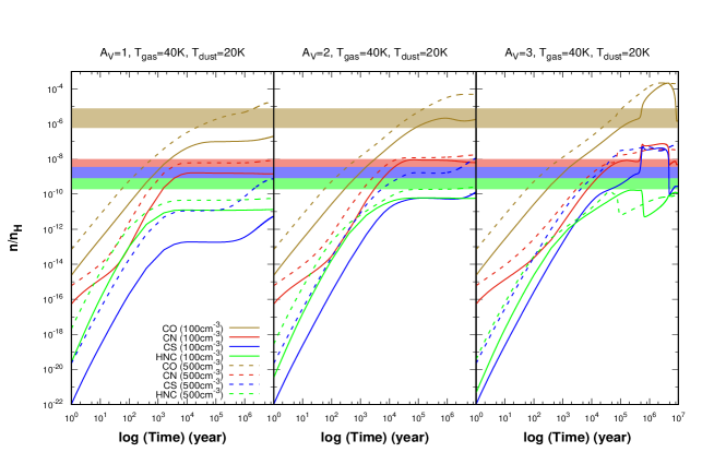
Figure 8: Time evolution of the abundances of CO, CN, CS, and HNC with the CMMC code for diffuse cloud. Observed abundances are also highlighted for the better understanding. The solid curves represent the case with $n_{H}=100$ cm^-3 and dashed curves represent the case with $n_{H}=500$ cm^-3.

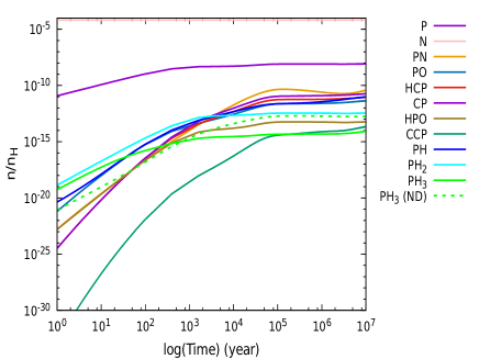
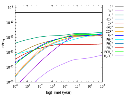
Figure 9: Chemical evolution of the P-bearing molecules for $A_{V}=2$ mag, $n_{H}=300$ cm^-3, $T_{gas}=40$ K, and $T_{dust}=20$ K with the CMMC code for diffuse cloud is shown. The evolution of the neutrals and radicals are shown on the left whereas ions are shown on the right side. Derived abundances of all the species are found to be $<10^{-10}$ for such condition.

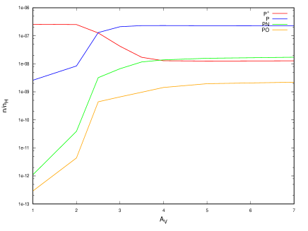
Figure 10: The final abundance of P⁺, P, PO, and PN are shown with A_V with the CMMC code for diffuse cloud. The conversion of P⁺ to P takes place in the range $A_{V}=2-3$ mag. Beyond A${}_{V}=4$ mag no changes in the abundances of P⁺ and P are obtained. The abundance ratio of PO and PN is found to be always $<1$.

We consider the initial elemental abundances for the diffuse cloud model as in Chantzos et al. (2020) (see Table 4). The dust to gas ratio of $0.01$ is considered in our model. We consider a photodesorption rate of $3\times 10^{-3}$ molecules per incident UV photon for all the molecules. Öberg et al. (2007) experimentally derived this rate from the laboratory measurement of CO ice. A non-thermal desorption constant $a=0.01$ and a cosmic ray ionization rate of $1.7\times 10^{-16}$ s^-1 are considered. We keep the gas and dust temperatures constant at $40$ K and $20$ K, respectively.

Figure 8 represents the results obtained with the CMMC code for the diffuse cloud region. The solid curve in the Figure represents the case when we consider $n_{H}=100$ cm^-3 and the dotted curve represents the case when we consider $n_{H}=500$ cm^-3. Figure 8 depicts that in the ranges of $A_{V}=2-3$ mag, and n${}_{H}=100-500$ cm^-3, we have a better agreement with the observed abundance.

Based on the obtained results, Figure 9 shows the chemical evolution of most of the P-bearing species considered in this study. In our case, we did not have a high abundance of PH₃ under this situation. It is because of the inclusion of the destruction pathways of PH₃ by H and OH in our network. The dashed green curve shows the PH₃ when we do not consider its destruction by H and OH in gas and ice both the phases. It is interesting to note that we have a couple of orders higher abundance of PH₃ in the absence of these destruction pathways. However, these destruction pathways are essential and need to be considered before constraining the PH₃ abundance. The right panel of Figure 9 depicts that the abundance of P⁺ remains constant for this case. Figure 10 shows the final abundance of P and P⁺ with a variation of $A_{V}$. It shows that P⁺ to P conversion is possible between $A_{V}=2-3$ mag and remains invariant beyond $A_{V}>4$ mag. For this case, we always get a higher peak abundance of PN compared to PO. At the end of the simulation, Chantzos et al. (2020) also obtained a comparatively higher abundance of PN than PO. With the Cloudy code, in Figure 4, we also have obtained PO/PN $<1$. The major difference between the CMMC model or the model used by Chantzos et al. (2020) and the Cloudy code is the consideration of the physical condition. The Cloudy code considers physical conditions more realistically. Figure 5 (diffuse cloud results with Cloudy) shows a substantial temperature variation with $A_{V}$, whereas in the case of the CMMC model, we assume a constant temperature ($T_{gas}=40$ K and $T_{ice}=20$ K) for all $A_{V}$. In the CMMC model, dust to gas ratio of $\sim 0.01$ is considered, whereas in the diffuse cloud model using Cloudy, it gives $6.594\times 10^{-3}$.

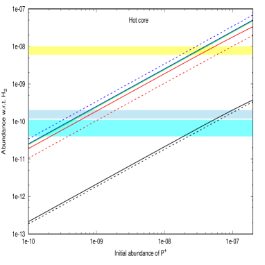
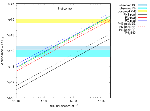
Figure 11: The observed abundances of PO and PN in the high mass star-forming region W51 and W3(OH) (Rivilla et al., 2016) are shown along with our modeled peak abundances (taken beyond the isothermal phase) with hot core (left panel) and hot corino (right panel) cases of our CMMC model. The peak abundance variation of the PH₃ is also shown with the initial abundance of P⁺. PH₃ is yet to be observed in hot core/corino. The obtained peak abundance of PH₃ is far below the observed limit of PH₃ in C-star envelope IRC +10216 (Agúndez et al., 2008, 2014). Peak abundances of PO, PN, and PH₃ are also shown with the dashed lines when the BE of the P-bearing species is considered from the tetramer configuration noted in Table 1. The solid green curve shows the peak abundance of PH₃ in the absence of its destruction by H and OH. We obtained a significantly higher peak abundance of PH₃ with the lack of these destruction pathways.

Table 5: Initial elemental abundance for the hot core/corino model considered in the CMMC code (Wakelam & Herbst, 2008).

Element	Abundance	Element	Abundance
H2	$0.5$	Fe+	$3.00\times 10^{-9}$
He	$1.40\times 10^{-1}$	Na+	$2.00\times 10^{-9}$
N	$2.14\times 10^{-5}$	Mg+	$7.00\times 10^{-9}$
O	$1.76\times 10^{-4}$	Cl+	$1.00\times 10^{-9}$
C+	$7.30\times 10^{-5}$	P+	$2.00\times 10^{-10}$
S+	$8.00\times 10^{-8}$	F+	$6.68\times 10^{-9}$
Si+	$8.00\times 10^{-9}$	e-	$7.31\times 10^{-5}$

4.2.2 Hot core / Hot corino model

Here, we consider a 3-phase starless collapsing cloud model described in Gorai et al. (2020). The first phase corresponds to an isothermal ($T_{dust}=T_{gas}=10$ K) collapsing phase where density can increase from $3\times 10^{3}$ cm^-3 to $10^{7}$ cm^-3 and visual extinction parameter ($A_{V}$) can increase from $2$ to $200$. The second phase corresponds to a warm-up phase where temperature rises from 10 to 200 K keeping $A_{V}$ constant at its maximum value in $5\times 10^{4}$ years. The last phase is a post-warm-up phase where density, temperature, and visual extinction are constant at their respective highest values and continue for $10^{5}$ years. Based on the time scale of the initial isothermal collapsing phase, we define the hot core and hot corino case. In the hot core case, we use an isothermal collapsing time scale $\sim 10^{5}$ years, whereas, for the hot corino case, a relatively longer timescale ($\sim 10^{6}$ years) is used. Thus, the total simulation time scale of $2.5\times 10^{5}$ years and $1.15\times 10^{6}$ years is considered for the hot core and hot corino cases, respectively. Table 5 shows the low metallic initial elemental abundance (Wakelam & Herbst, 2008), which is considered here.

Rivilla et al. (2016) reported the observed molecular abundance with an uncertainty of $\sim(0.5-5)\times 10^{-10}$ for PO and PN. The ratio between PO and PN varies in the range $1-5$. Figure 11 shows the variation of the peak abundance of PO and PN in the case of hot core and hot corino by considering various initial elemental P abundances. The peak abundances of PN and PO from our hot core (left panel) model shows a good match with the observation toward the massive star-forming region when an initial elemental P abundance (P⁺ abundance) of $2\times 10^{-10}-2\times 10^{-9}$ is considered.

The solid curve of Figure 11 represents the BE of the P-bearing species as it is in KIDA. The dashed curve represents our computed BE values (BE with water c-tetramer) of phosphorous (see the BE values in Table 1) and keeps all other BE values the same as in KIDA. We notice an increase in the peak abundances of PO and PN for the inclusion of our calculated BEs for the hot corino case. We have obtained that the peak abundance of PN increases, whereas it decreases for PO for the hot core case. PO’s peak abundance is always more prominent than the peak abundance (beyond the isothermal phase) of PN in both cases. Variation of the PH₃ abundance is also shown, which is far below the derived upper limit for the C-rich envelop Agúndez et al. (2008, 2014). The changes in BE reflects a significant increase in the gas phase abundance of PH₃ for the hot corino case, but a marginal decrease in the peak abundance of PH₃ is obtained in the case of the hot core. Additionally, in Figure 11, PH₃ abundance is shown with a solid-green curve (with the BE of KIDA) when its destruction by H and OH is not included. It offers a significantly higher abundance of PH₃.

Unless otherwise stated, we always use a non-thermal desorption factor of $a=0.01$. Additionally, we have tested with a reactive desorption factor of $0.023$ (Nguyen et al., 2020) for PH₃, which yields roughly $2.3$ times higher abundance of PH₃ in our case.

The solid lines of Figure 12 show the time evolution of the abundances of PO and PN and PO/PN for the hot core (upper panel) and hot corino (lower panel) case. The dashed lines represent the time evolution of the abundances of PO, PN, and the ratio PO/PN by considering the BEs of P-bearing species with the tetramer configuration of water. For a better understanding, we highlight the observed abundances and observed abundance ratio in the high mass star-forming region by Rivilla et al. (2016). For the hot core case, we consider the initial P⁺ abundance $\sim 1.8\times 10^{-9}$, and for the hot corino case, a comparatively higher initial abundance of P⁺ ($\sim 5.6\times 10^{-9}$) is considered to match the observational result. We have obtained an exciting difference between the PO and PN abundances during the later stages of the simulation of the post-warm-up phase. We have got PO/PN $>1$ in the post-warm-up phase (latter stage of this phase) of the hot core, whereas it shows an opposite trend in the hot corino case. The higher abundance of PN in the hot corino case happens due to the presence of a comparatively more elevated amount of atomic nitrogen (shown in Figure 12 with the pink curve) in this case. This high abundance of atomic nitrogen undergoes $\rm{PO+N\rightarrow PN+O}$ and yields PO/PN $<1$ in the hot corino case. Also, the abundance of atomic P increases due to the destruction of P-compounds. Our modeling results for hot core (with PO/PN $>1$) and hot corino (with PO/PN $<1$) agree well with the modeling results presented by Jiménez-Serra et al. (2018). The peak abundance of Figure 13 shows the time evolution of most of the P-bearing species with an initial P⁺ abundance of $1.8\times 10^{-9}$. It is interesting to note that at the end of the simulation time scale, mainly P is locked in the form of PO and PN.

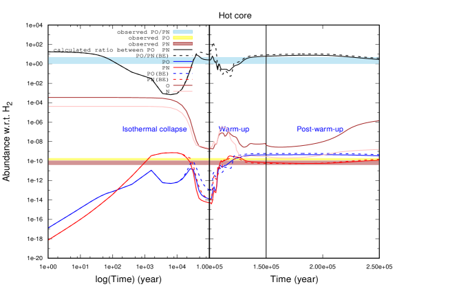
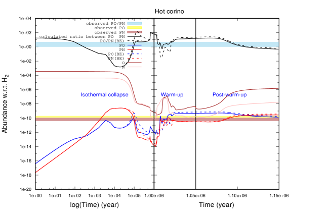
Figure 12: Abundance variation of PO, PN, and PO/PN ratio obtained from our CMMC model by considering the initial elemental abundance of P⁺ as $1.8\times 10^{-9}$ for hot core and $5.6\times 10^{-9}$ for the hot corino case. Solid lines represent the cases with the BEs from KIDA, and the dashed lines represent the values with the tetramer configuration of water. During the warm-up and post-warm-up phases, we have a good correlation with our results.

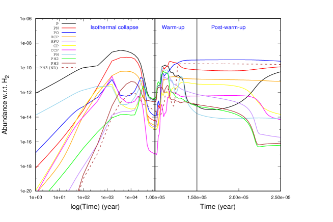
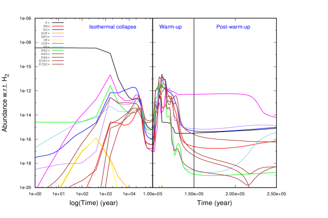
Figure 13: Abundance variation of most of the P-bearing neutral and ionic species are shown from our CMMC model considering initial elemental abundance of P⁺ as $1.8\times 10^{-9}$ and for hot core region. In the absence of the destruction of PH₃ by H and OH, PH₃ is highly abundant.

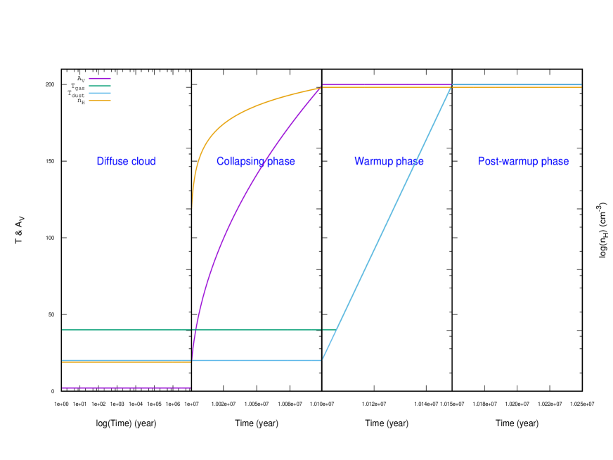
Figure 14: Here, in our CMMC model, we consider four distinct phases for this simulation. In the first phase, the cloud remains in the diffuse stage for $10^{7}$ years. It starts to collapse in the next step, which continues for $10^{5}$ years. The collapsing phase is followed by a warm-up and post-warm-up phase, which continues for another $1.5\times 10^{5}$ years.

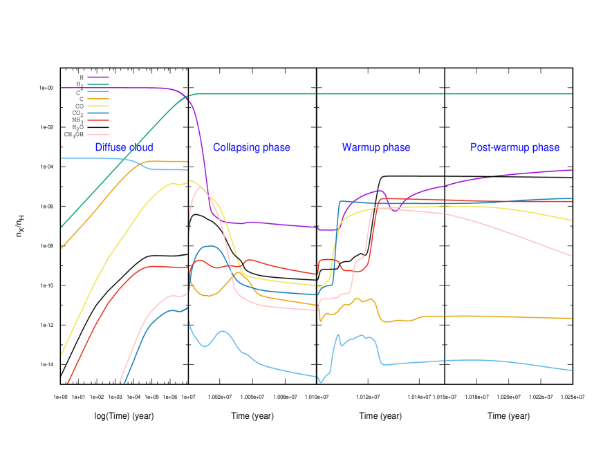
Figure 15: Time evolution of H, H₂, C⁺, C, CO, CO₂, NH₃, H₂O, and CH₃OH obtained from our CMMC model is shown. During the lifetime of the diffuse cloud H converts into H₂ and C⁺ converts into C. During the collapsing phase, C atom is heavily depleted and converts into CO.

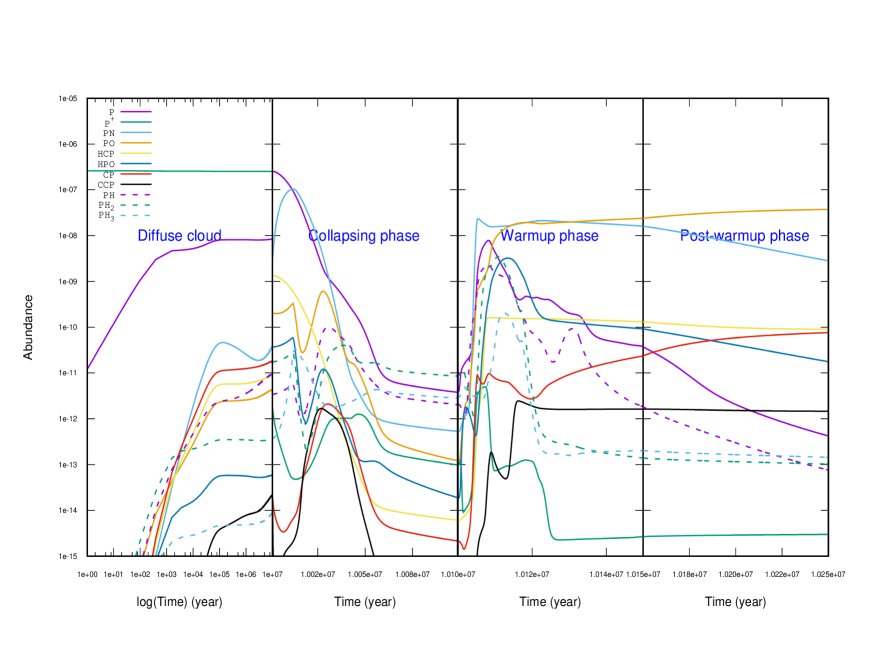
Figure 16: Time evolution of the abundances (with respect to total hydrogen nuclei in all forms) of major P-bearing species from our CMMC model is shown.

4.2.3 Diffuse to Dense cloud model

To avoid any ambiguity for considering the depletion factor, here we consider that the diffuse cloud converts into a molecular cloud after a sufficient time. The adopted physical condition for this model is shown in Figure 14. It depicts that the total simulation time is divided into four steps. The first step is the diffuse phase, and it continues for the initial $10^{7}$ years. The second step is the collapsing phase, whose span is for $10^{5}$ years. The warm-up phase starts after the collapsing phase, and it lasts for $5\times 10^{4}$ years. Finally, the post-warm-up phase continues for another $10^{5}$ years. In total, the simulation time scale is $1.025\times 10^{7}$ years. Initial elemental abundance for this case was taken from Chantzos et al. (2020) (see Table 4). All the BEs are used from the KIDA database. Figure 15 shows the time evolution of the H, H₂, C⁺, C, and CO. It is interesting to note that during the lifetime of the diffuse cloud ($\sim 10^{7}$ years), most of the H atoms convert into H₂. Ionized carbon is converted into neutral carbon. During the collapsing phase, the conversion of C to CO takes place. Once CO has formed, it starts to deplete on the grain and forms complex organic molecules (COMs). In the warm-up phase, these CO and its related molecules desorbed back to the gas phase. Figure 16 shows the chemical evolution of the notable P-bearing species. Figure 16 shows that in the warm-up phase, we have very high abundances of PN and PO. The abundance PH₃ is also significantly higher ($\sim 10^{-10}$ with respect to total H nuclei) comparable with Jiménez-Serra et al. (2018). At the end of the simulation, we see that most of the P is locked in the form of PO and PN.

Table 6: Peak abundances of the P-bearing species under various physical condition. The bracketed values in the CMMC model denote the case when the destruction of PH₃ by H and OH are ignored.

Species	Cloudy output		CMMC output
	Diffuse cloud ($n/n_{H}$)	PDR ($n/n_{H}$)	Diffuse cloud ($n/n_{H}$)	Hot core $(n/n_{H_{2}}$)	Hot corino $(n/n_{H_{2}}$)	Diffuse-Dense ($n/n_{H_{2}}$)
	($A_{V}=2$, $n_{H}=300$ cm-3)	($A_{V}=5$, $T_{gas}=50$ K, $T_{ice}=20$ K	($A_{V}=2$, $T_{gas}=40$ K, $T_{ice}=20$ K	(initial P${}^{+}\sim 1.8\times 10^{-9}$)	(initial P${}^{+}\sim 5.6\times 10^{-9}$)	(initial P${}^{+}\sim 2.6\times 10^{-7}$)
		$n_{H}=10^{5.5}$ cm-3)	$n_{H}=300$ cm-3)
PN	$3.33\times 10^{-10}$	$4.02\times 10^{-09}$	$4.6\times 10^{-11}$	$1.7\times 10^{-10}(2.9\times 10^{-11})$	$1.4\times 10^{-10}(8.0\times 10^{-11})$	$1.04\times 10^{-7}$
PO	$1.47\times 10^{-10}$	$2.60\times 10^{-11}$	$4.4\times 10^{-12}$	$2.3\times 10^{-10}(4.9\times 10^{-11})$	$2.6\times 10^{-10}(6.6\times 10^{-11})$	$3.7\times 10^{-8}$
PH	$1.13\times 10^{-10}$	$1.82\times 10^{-11}$	$9.6\times 10^{-12}$	$5.5\times 10^{-11}(1.5\times 10^{-11}$)	$6.5\times 10^{-11}(8.9\times 10^{-12})$	$2.3\times 10^{-9}$
PH3	$6.30\times 10^{-31}$	$1.16\times 10^{-22}$	$8.9\times 10^{-15}$	$1.9\times 10^{-12}(2.1\times 10^{-10})$	$9.2\times 10^{-12}(2.3\times 10^{-10})$	$2.0\times 10^{-10}$
CP	$2.03\times 10^{-11}$	$3.24\times 10^{-12}$	$1.8\times 10^{-11}$	$3.5\times 10^{-12}(6.7\times 10^{-13})$	$3.1\times 10^{-11}(3.2\times 10^{-12})$	$1.2\times 10^{-10}$
HCP	$1.38\times 10^{-13}$	$3.85\times 10^{-14}$	$9.1\times 10^{-12}$	$9.5\times 10^{-12}(3.7\times 10^{-12})$	$3.5\times 10^{-11}(4.3\times 10^{-12})$	$1.3\times 10^{-9}$
HPO	$4.43\times 10^{-17}$	$1.28\times 10^{-19}$	$5.9\times 10^{-14}$	$1.2\times 10^{-11}(1.6\times 10^{-12})$	$1.5\times 10^{-11}(9.8\times 10^{-13})$	$3.2\times 10^{-9}$

Table 7: Summary of the obtained abundance ratio between PO and PN in different astrophysical environment.

References	Type of study	PDR	Diffuse cloud	Hot core	Hot corino	Shock	Comet	Other
This work	Modeling	$<<1$	$<1$	$\geq 1^{l}$	$\geq 1^{m}$, $\leq 1^{n}$	$\cdots$	$\cdots$	$\cdots$
Bernal et al. (2021)	Observation	$\cdots$	$\cdots$	$\cdots$	$\cdots$	$\cdots$	$\cdots$	2.7a
Rivilla et al. (2020)	Observation	$\cdots$	$\cdots$	$\cdots$	$\cdots$	$\cdots$	$>10^{b}$	1.7c
Chantzos et al. (2020)	Modeling		$<1$
Bergner et al. (2019)	Observation	$\cdots$	$\cdots$	$\cdots$	$\cdots$	$\cdots$	$\cdots$	$(1-3)^{d}$
Rivilla et al. (2018)	Observation	$\cdots$	$\cdots$	$\cdots$	$\cdots$	$\cdots$	$\cdots$	$\sim 1.5^{e}$
Jiménez-Serra et al. (2018)	Modeling	$<<1$	$\cdots$	$\geq 1$	$<1$	$\leq 1$	$\cdots$	$\cdots$
Lefloch et al. (2016)	Observation	$\cdots$	$\cdots$	$\cdots$	$\cdots$	$\approx 3^{f}$	$\cdots$	$\cdots$
Rivilla et al. (2016)	Observation	$\cdots$	$\cdots$	$1.8^{g}$, $3^{h}$	$\cdots$	$\cdots$	$\cdots$	$\cdots$
Fontani et al. (2016)	Observation	$\cdots$	$\cdots$	$\cdots$	$\cdots$	$\cdots$	$\cdots$	$<(1.3-4.5)^{i}$
De Beck et al. (2013)	Observation	$\cdots$	$\cdots$	$\cdots$	$\cdots$	$\cdots$	$\cdots$	$0.17-2^{j}$
Aota & Aikawa (2012)	Modeling	$\cdots$	$\cdots$	$\cdots$	$\cdots$	$\sim(0.5-1.3)^{f,i}$	$\cdots$	$\cdots$
Tenenbaum et al. (2007)	Observation	$\cdots$	$\cdots$	$\cdots$	$\cdots$	$\cdots$	$\cdots$	$2.2^{k}$

Note. — ^a Orion-KL, ^b 67P/Churyumov-Gerasimenko (Altwegg et al., 2016).

^c Average over multiple positions and velocity components toward AFGL 5142.

^d Class I low-mass protostar B1-a.

^e G+0.693-0.03, ^f L1157-B1, ^g W51 e1/e2, ^h W3(OH).

ⁱ Taking minimum and maximum values of upper limit of beam-averagd column densities of multiple sources.

^j IK Tauri, ^k VY Canis Majoris.

^l For the late warmup to post warmup phase of the hot core model.

^m During the late warm-up to the initial post-warm-up of hot corino phase.

ⁿ During the late post warm-up phase.

4.3 An outline of our modeling results and a comparison with the earlier results

Table 6 shows the peak abundances of the significant P-bearing species obtained with the two models (Cloudy and CMMC). However, due to more realistic physical conditions, the Cloudy code is preferred for the diffuse cloud region. Both the diffuse cloud models (Cloudy and CMMC) show that PN’s abundance is higher than that of PO. Chantzos et al. (2020) also predicted a higher abundance of PN ($4.8\times 10^{-11}$) compared to PO ($1.4\times 10^{-11}$) in the diffuse cloud region. The abundances of PH₃ dramatically vary between the two models; this is because Cloudy does not consider the grain surface reactions for the formation of PH₃, whereas the grain chemistry is adequately considered in CMMC. Moreover, the adopted physical condition differs between the two models. We have obtained a higher abundance of P-bearing species for our diffuse-dense model because of the consideration of the initially high abundance of P⁺ ($\sim 2.6\times 10^{-7}$). In general, we have obtained a nice trend with the peak abundance ratio between PO and PN. We find PO/PN ratio $<1$ for the diffuse cloud region, $<<1$ for the PDR region, and $>1$ for the hot core/cornio (late warm-up phase) region. In the late post-warm-up phase, we have PO/PN $>1$ for hot core and $<1$ for the hot corino. We have noticed that the reaction $\rm{PO+N\rightarrow PN+O}$ is mainly responsible for controlling this ratio.

The results of our diffuse cloud modeling with the Cloudy and CMMC code is in line with that obtained by Chantzos et al. (2020). The significant difference between our diffuse cloud model with the Cloudy code and the model presented in Chantzos et al. (2020) is in consideration of realistic physical conditions instead of just considering the constant temperature. In contrast, the diffuse cloud model with CMMC code adopted similar physical parameters considered in Chantzos et al. (2020). Since Cloudy was not equipped with adequate surface chemistry treatment, we did not have a notable abundance of PH₃. Our CMMC results show lower PH₃ because of its destruction by H and OH.

Charnley & Millar (1994) studied the chemistry of P in hot molecular cores. They considered that the gas phase P-chemistry in the hot core starts from PH₃ release from the interstellar grains. In their case, PH₃ was gradually destroyed and transformed into P, PO, and PN. They noticed that other P-bearing species formation time scale is longer than those of the hot core. We consider the in situ formation of PH₃ via chemical reaction on interstellar grains. Like Charnley & Millar (1994), in Figure 13, we also notice that at the end of the warm-up phase, the abundances of most of the P-bearing species remain in the form of P, PO, and PN.

Rivilla et al. (2016) found that PO and PN are chemically associated and formed during the cold collapse phase by the gas phase reactions. At the end of the collapsing phase, these two species were deposited to the interstellar grain. These again desorb back to the gas phase during the warm-up phase when the temperature is around 35 K. Our CMMC model shown in Figure 12 shows the similar behavior of PO and PN. In the isothermal collapsing phase, the gas-phase abundance of these two species offers a higher abundance, while at the end of this phase, these two are depleted to the grain. Once the temperature has become $>35$ K in the warm-up phase, it desorbed back to the gas phase.

Jiménez-Serra et al. (2018) constructed their model to explain the abundances of P-bearing species in a wide range of astrophysical conditions. They constructed a short-lived and long-lived chemical model depending on the time of the collapse. In the short-lived collapse, they stopped their calculations when the gas density reaches its maximum value. In the long-lived collapse, they considered some additional time after getting the final density. They noticed that the P and PN are the most abundant phosphorous-bearing species in the collapsing phase. Their maximum abundance varies in the range $(5-10)\times 10^{-10}$. From our hot core model, in the collapsing phase (see Figure 13), we also have obtained that P and PN remain the most abundant P-bearing species, and their peak abundance varies in the range $(7-27)\times 10^{-10}$.

Jiménez-Serra et al. (2016) carried out a high sensitivity observation toward the L1544 pre-stellar core. They were not able to identify the PN transitions. However, they predicted an upper limit of $\sim 4.6\times 10^{-13}$ for the abundance of PN. The first phase of Figure 13 represents the isothermal collapsing phase of a hot core. At the end of the collapsing phase, we have obtained a PN abundance of $\sim 5.4\times 10^{-15}$, which is consistent with this upper limit. Fontani et al. (2016) identified PN in various dense cores, which are in different evolutionary stages (starless, with a protostellar object, and with ultracompact H II region) of the intermediate and high-mass star formation. They obtained all the transitions of PN where the temperature is $<100$ K, and linewidths are $<5$ km s^-1, suggesting that the origin of PN in the quiescent and cold region. Because of the lack of data of the thermal dust continuum emission (at the millimeter/submillimeter regime for all these sources), PN’s abundances were not derived. Mininni et al. (2018) identified a few transitions of PN toward some of these sources (a sample of nine massive dense cores in different evolutionary stages). They had calculated the H₂ total column densities of the sources and derived the abundances of PN. For the slightly warmer region ($25-30$ K), Fontani et al. (2016) and Mininni et al. (2018) obtained $10^{-11}$ and $5\times 10^{-12}$, respectively. Our Figure 13 depicts that when the temperature is $\sim 35$ K in the warm-up phase, we have a little higher PN abundance $\sim 2.08\times 10^{-11}$ with respect to H₂. The main reason behind this difference is that. Mininni et al. (2018) found the excitation temperature of PN $\sim 5-30$ K. Since the average density ($\sim 10^{4-5}$ cm^-3) of their targeted regions are below the critical density ($10^{5-6}$ cm^-3) of the PN, they suggested a sub thermal excitation of PN. The total hydrogen density can reach as high as $10^{7}$ cm^-3 in our isothermal phase. In the warm-up phase, we have considered the same density. So in our case, we have an average density, which is greater than the critical density of PN. So, a direct comparison between our model and the observation of Mininni et al. (2018) and Fontani et al. (2016) would not be appropriate. Here, we have referred to these observations to infer the enhancement of the PN abundance with the increase in temperature from $10$ K to $35$ K only.

After releasing to the gas phase, PH₃ can destroy rapidly (Jiménez-Serra et al., 2018). The gas-phase formation of PH₃ can continue by the reactions R144 and R145 of Table 10 (in the Appendix). These two reactions were considered in Jiménez-Serra et al. (2018) and found to contribute marginally. Here, we have some additional destruction reactions of PH₃ by H (grain phase reaction R4 and gas-phase reaction R149 of Table 10) and OH (grain phase reaction R5 and gas-phase reaction R161 of Table 10) which yields a much lower PH₃ in the gas phase.

In Table 7, a summary of PO/PN abundance ratio is listed in the different astrophysical environments, along with a comparison with the earlier literature (Bernal et al., 2021; Rivilla et al., 2020; Chantzos et al., 2020; Bergner et al., 2019; Jiménez-Serra et al., 2018; Rivilla et al., 2018, 2016; Lefloch et al., 2016; Fontani et al., 2016; De Beck et al., 2013; Aota & Aikawa, 2012; Tenenbaum et al., 2007). Our modeling results agree well with the observed (Rivilla et al., 2016) and modeled (Jiménez-Serra et al., 2018; Chantzos et al., 2020) PO/PN ratios.

5 1D-RATRAN radiative transfer model

Here, we employ a 1D radiative transfer model (Hogerheijde & van der Tak, 2000) to look into the transitions from the notable P-bearing species in the diffuse cloud region and around the more evolved stage, the hot core/corino region.

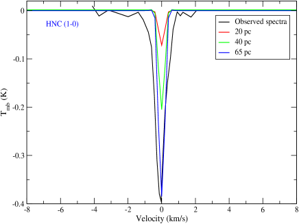
Figure 17: Modeled $1\rightarrow 0$ transitions of HNC by considering the different sizes of the diffuse cloud in the RATRAN model. It is interesting to note that the intensity of the absorption increases with the increase in the size of the cloud. Abundance of $2\times 10^{-10}$ and Doppler parameter of 0.2 km/s are used.

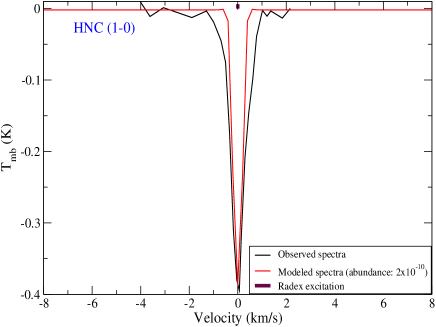
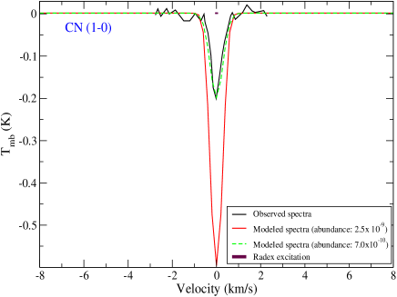
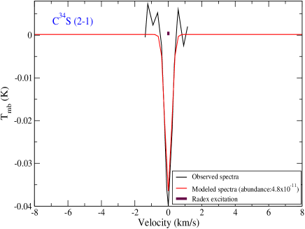
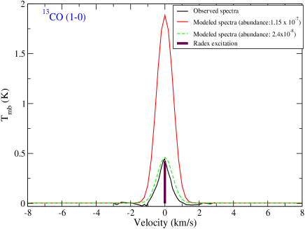
Figure 18: Modeled line profile (with the RATRAN code) of HNC (1-0), CN (1-0), C³⁴S (2-1), and ¹³CO (1-0) for the diffuse cloud region. The black curve represents the observed line profile, whereas the red curve shows the modeled line profiles. Here, we consider H and H₂ as the collision partners having number density $100$ and $400$ cm^-3 for H and H₂ respectively. A temperature of $70$ K is considered for both gas and ice phases. The maroon vertical line shows the excitation with RADEX.

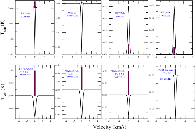
Figure 19: Modeled line profile (with the RATRAN code) of PN, HCP, PO which can be observed in the diffuse cloud region. The black curve represent the modeled spectra whereas the maroon line represents the line excitation using RADEX. Here, we consider H and H₂ as the collision partners having number density $100$ and $400$ cm^-3 for H and H₂ respectively. A temperature of $70$ K is considered for both gas and ice phases.

5.1 Diffuse cloud model

Here we model the galactic diffuse cloud region present in the line of sight toward the strong continuum source B0355+508 (Chantzos et al., 2020). We divide the entire cloud into $23$ spherical shells. Since around the diffuse cloud region, hardly a few mono-layers of ice could survive, we consider a dust absorption coefficient with the bare grain (MRN model with no ice mantle) with a coagulation time of $10^{8}$ years (see Table 1 of Ossenkopf & Henning, 1994). We have used the dust emissivity ($\kappa$) by considering a power-law emissivity model.

$$\kappa=\kappa_{0}(\nu/\nu_{0})^{\beta},$$ (3)

where $\kappa_{0}$=1520 cm²/gm and $\nu_{0}$=1.62$\times$10¹³ Hz (Ossenkopf & Henning, 1994). The power-law index $\beta$ is considered $\sim 1.0$. We have run several cases varying the number density of the collision partners (atomic and molecular hydrogen), the kinetic temperature of the gas, abundance profile, the Doppler broadening parameter, size of the cloud, etc. The diffuse cloud model discussed in the earlier section shows that at the end of the simulation ($\sim 10^{7}$ years), a significant portion of hydrogen would convert into H₂. Keeping this in mind, we consider $\rm{n_{H}=100}$ cm^-3 and $\rm{n_{H_{2}}=400}$ cm^-3 for this simulation.

In Figure 17, we show the absorption profile of the $1\rightarrow 0$ transition of HNC as obtained from the 1D RATRAN model. Here, we consider the different sizes of the cloud to represent the absorption observed by Chantzos et al. (2020). We notice that with the increase in the size of the cloud, the absorption is getting stronger. For the 65 pc size, we obtain a good match with the observed intensity. We use an abundance of $2\times 10^{-10}$ and the Doppler parameter of $\sim 0.2$ km/s for HNC. In Figure 18, the extracted observed spectra of HNC(1-0), CN (1-0), C³⁴S (2-1) and ¹³CO (1-0) (Chantzos et al., 2020) in black, along with the modeled spectra in red, are shown. It is interesting to note that with the chosen parameter, we can successfully explain the absorption features of HNC, CN, and C³⁴S and emission feature of ¹³CO.

In contrast to the modeling result of Chantzos et al. (2020) and the modeling results discussed in the earlier sections above, a combination of higher gas temperature ($\sim 70$ K) and density is required to explain the observed line profiles. We consider the gas and dust temperature to be equal in our calculation. Here, we use the collisional data file in the LAMDA database for HNC, CN, ¹³CO with H₂. No collisional rates with H were available. For simplicity, we consider it to be the same as it is with H₂. We further have tested using the scaled rate for H (Schöier et al., 2005), no significant difference in synthetic spectra is observed. Since the collisional data file of C³⁴S was not available, we consider it similar to the C³²S from the LAMDA database. We obtain the best-fitted Doppler broadening parameter of 0.2, 0.4, 0.25, and 0.592 km/s for HNC, CN, C³⁴S, and ¹³CO, respectively, are consistent with the FWHM values obtained by Chantzos et al. (2020). It is to be noted that our results can simultaneously explain the absorption features of HNC, CN, C³⁴S, and the emission feature of ¹³CO.

Here, we convolve the synthetic spectra with the perfect beam size obtained for IRAM-30m observation. We obtain a best-fitted abundance of $\sim 2\times 10^{-10}$ for HNC. Chantzos et al. (2020) obtained an abundance of HNC $\sim 2.1\times 10^{-10}$ from the modeling. Chantzos et al. (2020) calculated ³²S/³⁴S isotopic ratio for the $-17$ km/s cloud is $18.7$, and ¹²CO/¹³CO isotopic ratio is $16.7$. Considering this fractionation ratio, the abundance ratio predicted by Chantzos et al. (2020) for HNC:CN:C³⁴S:¹³CO is $1:12.5:0.24:576.35$. Maintaining the same abundance ratio of Chantzos et al. (2020), we have $2.5\times 10^{-9}$, $4.8\times 10^{-11}$, and $1.15\times 10^{-7}$ for CN, C³⁴S, and ¹³CO, respectively. The modeled spectra with these abundances are shown in Figure 18 with the solid red lines. In the case of C³⁴S, we have an excellent match with this abundance. But for CN and ¹³CO, we have strong absorption and emission respectively with these abundances. For CN, an abundance of $7\times 10^{-10}$, and for ¹³CO, an abundance of $2.4\times 10^{-8}$ shows an excellent match (see the green dashed lines).

In Figure 19, the line profiles of the P-bearing species PN, HCP, and PO in the diffuse cloud region are shown. Using the same diffuse cloud model and considering abundances obtained from the CMMC model, i.e., $4.6\times 10^{-11}$ for PN, $9.1\times 10^{-12}$ for HCP, and $4.4\times 10^{-12}$ for PO, we generate the synthetic spectra for these three P-bearing molecules. For this purpose, we use the Doppler parameter to be $0.3$ km/s for PN, HCP, and PO, respectively, from Chantzos et al. (2020) which is consistent with the low FWHM values observed for other molecules in the diffuse cloud. The collisional data for HCP and PN are taken from Basecol database. The collisional rate of PO was taken from the LAMDA database. The collisional rate with the H atom is considered to be the same as it is with H₂. For the IRAM-30m telescope, the beam convolution is considered using the beam sizes mentioned in the Appendix Section B (see Tables 11, 12, 13, 14). Interestingly, for PN and PO, we have obtained the spectra in absorption, whereas for the HCP, we have obtained it in emission. To further check the excitation condition for the molecules observed and the phosphorus-bearing molecules targeted, we employ the RADEX code (van der Tak et al., 2007). For the RADEX calculation, we consider the column densities for HNC, CN, C³⁴S, ¹³CO as 0.69$\times$10¹², 0.87$\times$10¹³, 1.64$\times$10¹¹ and 3.98$\times$10¹⁴ cm^-2 and FWHM 0.73, 0.54, 0.43, 0.82 km/s respectively from table 4 of Chantzos et al. (2020) for the diffuse cloud at an offset velocity $\simeq$ -17 km/s with respect to the source. We consider the input kinetic temperature 40 K and number density of collision partner H as 300 cm^-3 and a very low H₂ density 10 cm^-3. A standard background of $2.73$ K is considered. In Figures 18 and 19, the line excitation obtained with the RADEX is shown with the maroon vertical line at the 0 km/s. Interestingly, in Figure 18, the excitation for HNC, CN, and C³⁴S (for which absorption was observed) is very weak for the previously observed molecules. In contrast, the excitation with the RADEX completely matches with the observed spectra for ¹³CO, observed in emission. Under the optically thin approximation and considering a very crude assumption, for the two-level system, the critical density can be represented by the ratio between the Einstein A coefficient in s^-1 and collisional rates in cm³ s^-1 (Shirley, 2015). In Table 8, we have noted down the Einstein A coefficient and collisional rate and critical density of these transitions. It is clear from the table that, as expected, we have obtained the transitions of HCP and ¹³CO in emission (critical density low) and the rest are in absorption (critical density high) with the RATRAN code (see Figures 18 and 19).

Table 8: Critical density of some transitions under the optically thin approximation.

Species	Transitions	Frequency	Einstein coefficient	Collision rate	Critical density
		(GHz)	(s${}^{-1})$	at $\sim 10$ K (cm${}^{3}s^{-1}$)	(cm-3)
CN	$N=1-0,\ J=1/2-1/2,\ F=3/2-1/2$	113.169	$1.182\times 10^{-5}$	$9.10\times 10^{-12}$	$1.299\times 10^{6}$
HNC	$J=1-0$	90.664	$2.69\times 10^{-5}$	$9.71\times 10^{-11}$	$2.770\times 10^{5}$
C34S	$J=2-1$	96.413	$1.60\times 10^{-5}$	$5.06\times 10^{-11}$	$3.162\times 10^{5}$
13CO	$J=1-0$	110.201	$6.294\times 10^{-8}$	$3.302\times 10^{-11}$	$1.906\times 10^{3}$
HCP	$J=2-1$	79.903	$3.61\times 10^{-7}$	$6.884\times 10^{-11}$	$5.244\times 10^{3}$
HCP	$J=3-2$	119.854	$1.31\times 10^{-6}$	$7.33\times 10^{-11}$	$1.786\times 10^{4}$
PN	$J=2-1$	93.979	$2.92\times 10^{-5}$	$4.538\times 10^{-11}$	$6.534\times 10^{5}$
PN	$J=3-2$	140.968	$1.05\times 10^{-4}$	$5.218\times 10^{-11}$	$2.012\times 10^{6}$
PO	$J=5/2-3/2,\ \Omega=1/2,\ F=3-2,\ e$	108.998	$2.132\times 10^{-5}$	$5.10\times 10^{-12}$	$4.179\times 10^{6}$
PO	$J=5/2-3/2,\ \Omega=1/2,\ F=2-1,\ e$	109.045	$1.92\times 10^{-5}$	$1.93\times 10^{-11}$	$9.952\times 10^{5}$
PO	$J=5/2-3/2,\ \Omega=1/2,\ F=3-2,\ f$	109.206	$2.143\times 10^{-5}$	$1.161\times 10^{-10}$	$1.846\times 10^{5}$
PO	$J=5/2-3/2,\ \Omega=1/2,\ F=2-1,\ f$	109.281	$1.93\times 10^{-5}$	$6.30\times 10^{-12}$	$3.062\times 10^{6}$

In Figure 19, line excitation of the P-bearing molecules are shown. The excitations obtained from the RADEX is well matched for HCP, which is in emission. For PN, we have seen emissions. For PO, we have obtained a strong emission with the RADEX, whereas the results obtained with the RATRAN code show these in absorption.

5.2 Hot core/corino model

Here, we execute a RATRAN radiative transfer model to explain the anticipated line profiles of the P-bearing molecules in the hot core/corino region. Rolffs et al. (2010) fitted the observed HCN profiles toward Sgr B2(M). They provided the best-suited spatially varying parameters (density, temperature, and velocity) for this case. Interestingly, they found that in-fall dominates in the outer parts, whereas multiple outflows were expelling matter from the inner region. Both density and temperature are almost linearly increasing toward the center of the hot core region. Using this physical parameter as input of the RATRAN model, we generate the synthetic spectra for different P-bearing molecules (PN, PO, HCP, and PH₃) for our hot core model. For the hot corino model, we also consider the same physical condition for simplicity (line profiles by considering more realistic physical requirements for the hot corino region are also reported in section C). For the first time, Rivilla et al. (2016) identified PO in the two star-forming regions W51 and W3(OH) in emission using the IRAM-30m telescope. Previously PO was detected in the envelope of the evolved stars but not in the star-forming regions. Rivilla et al. (2016) also recognized some transitions of PN in emission. They explained the observed column densities of PN and PO using a chemical model. We use the abundances of PO, PN, HCP, and PH₃ for the hot core/corino model from Table 6. Following Rolffs et al. (2010), here, we assume a bare dust grain (Ossenkopf & Henning, 1994) due to the high temperature of the source.

The massive hot core Sgr B2(M) is situated at a distance of $\simeq$ 7.8 kpc (Reid et al., 2009). Rivilla et al. (2016) obtained FWHM for PO and PN as 7.0 and 8.2 km/s, respectively. Based on these choices, here, we use line-broadening parameter (i.e., the Doppler parameter) for PO and PN as 4.2 and 4.9 km/s, respectively. For HCP, we consider it the same as PN (i.e., 4.9 km/s). For PH₃, we consider it 1.9 km/s. We consider the collisional data file for PN and HCP with H₂ from the BASECOL database (Dubernet et al., 2013). No collisional data files were available for PH₃. Looking at the structural similarity, we consider the H₂ collisional rate of NH₃ in place of PH₃. The same numerical values are considered for the hot corino case.

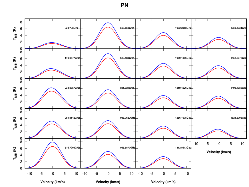
Figure 23: Table 11 shows possible transitions of PN, which could be observed with the IRAM-30m or SOFIA (GREAT) toward hot core/corino. The estimated line profile of these transitions obatined with the RATRAN model is shown here for hot core (blue) and hot corino (red) using the abundances from Table 6.

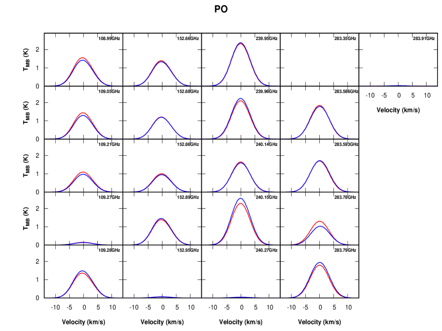
Figure 24: Table 12 shows the possible transitions of PO, which could be observed with the IRAM-30m toward Sgr-B2(M). The estimated line profile of these transitions with the RATRAN model is shown here for hot core (blue) and hot corino (red) using the abundances from Table 6.

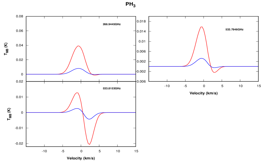
Figure 26: Table 14 shows the possible transitions of PH₃, which could be observed with the IRAM-30m and SOFIA (GREAT) toward Sgr-B2(M). The estimated line profile of these transitions with the RATRAN model is shown here for hot core (blue) and hot corino (red) using the abundances from Table 6.

We calculate the beam size for IRAM-30m and for SOFIA-GREAT. Estimated telescopic parameters (main beam temperature, beam size, integration time, and visibility) for the diffuse cloud and hot core/corino region are noted in Tables 11, 12, 13, and 14 for PN, PO, HCP, and PH₃ respectively. Only the potentially detectable transitions in the hot core/corino region are noted in the tables. The predicted line profiles of these transitions after performing beam convolution are shown in Figures 23, 24, 25, and 26 of the Appendix Section B. Interestingly, we have obtained “inverse P-Cygni type” spectral profiles for some transitions of PH₃ (see Figure 26). This unique type of velocity profile represents both in-fall and outflow are present in this source. Theoretically, Rolffs et al. (2010) predicted the existence of accelerating in-fall having a density power-law index of $\sim 1.5$ to support a spherically symmetric constant mass accretion rate in Sgr B2(M). However, they were also unable to obtain the observational evidence of accelerating infall. In Appendix Section C, we have shown the obtained line profiles when physical condition related to IRAS4A was considered as a representative of a hot corino case. We notice that the physical input parameters are very much susceptible to the derived line profiles. We do not obtain the inverse P-cygni profile while we use the physical parameters of IRAS4A. But it is out of scope for this work to comment elaborately on such concerns here.

Table 9: Experimental and calculated infrared data for PH₃.

Assignment	Frequency [cm-1]					Absorption Coefficients [cm molecule-1]
	Experimentala	Calculatedb		Calculatedb $\times$ 0.967		Experimentala	Calculatedb
		Harmonic	Anharmonic	Harmonic	Anharmonic		Harmonic	Anharmonic
Fundamental Bands
$\nu_{2}$ (bending)	982	1007.267	990.267	974.027	957.588	$0.51\times 10^{-18}$	$5.40\times 10^{-18}$	$5.11\times 10^{-18}$
$\nu_{4}$ (scissoring)	1096	1134.859	1110.02	1097.409	1073.389	$0.71\times 10^{-18}$	$2.78\times 10^{-18}$	$2.55\times 10^{-18}$
scissoring		1134.967	1103.681	1097.513	1067.260		$2.78\times 10^{-18}$	$2.58\times 10^{-18}$
$\nu_{1}$ (symmetric stretching)	2303	2396.887	2296.619	2317.790	2220.831	$2.4\times 10^{-18}$	$7.82\times 10^{-18}$	$7.86\times 10^{-18}$
$\nu_{3}$ (asymmetric stretching)	2316	2401.893	2303.377	2322.630	2227.366	$8.4\times 10^{-18}$	$1.38\times 10^{-17}$	$1.47\times 10^{-17}$
asymmetric stretching		2405.153	2283.634	2325.783	2208.274		$1.34\times 10^{-17}$	$1.45\times 10^{-17}$
Overtones
2$\nu_{4}$	2195		2213.024		2139.994			$2.98\times 10^{-19}$
3$\nu_{2}$	2905
2$\nu_{1}$	4536		4540.981		4391.129			$1.35\times 10^{-22}$
Combination Bands
$\nu_{2}+\nu_{4}$	2067, 2083		2093.256		2024.178			$2.86\times 10^{-20}$
$\nu_{1}/\nu_{3}+\nu_{L}$	2376, 2426, 2461
$\nu_{1}+\nu_{2}$	3288		3280.701		3172.438			$6.50\times 10^{-22}$
$\nu_{1}+\nu_{4}$	3392		3391.715		3279.788			$7.12\times 10^{-20}$
$\nu_{3}+\nu_{4}$	3405		3392.344		3280.397			$5.67\times 10^{-20}$
$\nu_{1}+\nu_{3}$	4621		4523.242		4373.975			$1.35\times 10^{-21}$

Note. — ^a Turner et al. (2015),

^b This work.

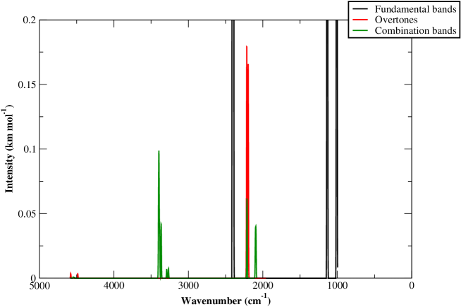
Figure 20: Ice phase IR absorption spectra of PH₃ including the harmonic fundamental bands and anharmonic overtones and combination bands.

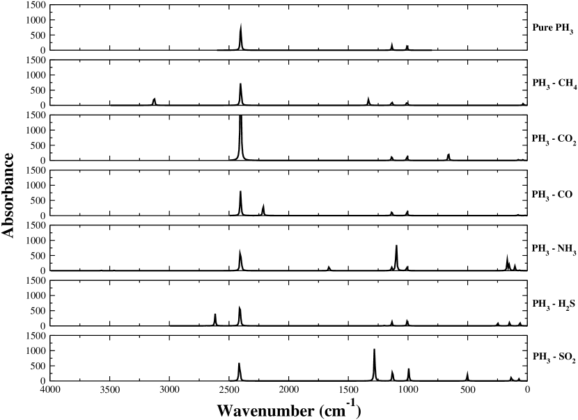
Figure 21: Comparison of ice-phase absorption spectra of pure PH₃ and mixture of PH₃ with other volatiles (CH₄, CO₂, CO, NH₃, H₂S, and SO₂) considering the harmonic fundamental bands.

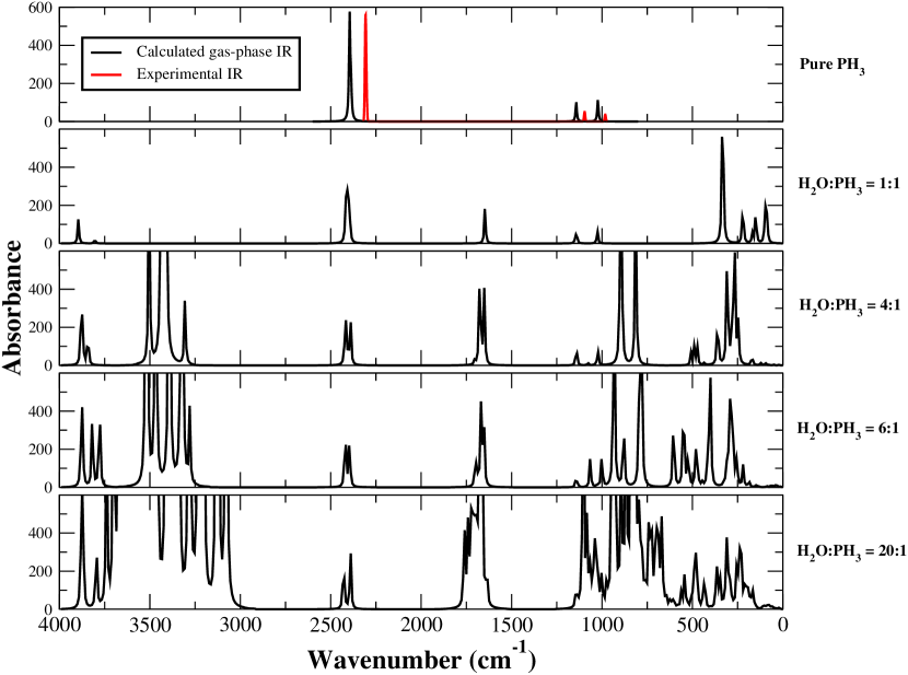
Figure 22: Gas-phase IR absorption spectra of PH₃ with increasing concentration of H₂O.

6 Infrared spectra of PH₃

Phosphine is an important reservoir of interstellar phosphorous (Charnley & Millar, 1994). Since it is of particular interest to astronomers, the IR vibrational spectra analysis of PH₃ could be helpful to the community. The vibrational spectra of PH₃ would be beneficial for future astronomical observations with the James Web Space Telescope (JWST). To precisely estimate the frequency and interpret the intensities, it is necessary to go beyond the harmonic approximation. The anharmonic calculations not only show a significant deviation from the harmonic calculations. Another advantage of the anharmonic analysis is that overtones and combination bands can also be analyzed with this. When anharmonicity is considered, their intensity vanishes at the harmonic level. The Density Functional Theory (DFT) is employed to investigate the IR feature of PH₃. Within the DFT approach, the standard B3LYP functional (Becke, 1993) has been used in conjunction with the 6-311G(d,p) basis set. All DFT computations have been performed employing the Gaussian suite of programs for quantum chemistry (Frisch et al., 2013). Figure 20 shows the calculated infrared feature of the ice phase PH₃. To mimic the ice features, the PH₃ molecule is embedded in a continuum solvation field to represent local effects. The integral equation formalism (IEF) variant of the polarizable continuum model (PCM) as a default self-consistent reaction field (SCRF) method is employed with water as a solvent (Cancès et al., 1997; Tomasi et al., 2005). The implicit solvation model places the molecule of interest inside a cavity in a continuous homogeneous dielectric medium representing the solvent. The fundamental modes of vibration, along with the overtones and combination bands, are shown in Figure 20. Table 9 also notes down the wavenumbers (in cm^-1) and corresponding absorption coefficients (IR intensities in cm molecule^-1) of the fundamental bands, overtones, and combination bands.

A comparison between our computed spectra and that obtained experimentally by Turner et al. (2015) is shown in Table 9. The computed vibrational frequencies are often scaled to resemble the experimental results. This scaling factor varies with the choice of the basis sets and implemented method. The NIST database noted some of the scaling factors, which are helpful to compare with the experimental values. Based on our method and the chosen basis set, we use a vibrational scaling factor of $\sim 0.967$. Puzzarini et al. (2014) demonstrated that the best state-of-the-art theoretical estimates have an accuracy of about $\rm{5\ cm^{-1}-10\ cm^{-1}\ and\ 10\ cm^{-1}-20\ cm^{-1}}$ for fundamental and non-fundamental transitions, respectively. This accuracy allows for reliable simulations of IR spectra supporting astronomical observations. The harmonic frequencies presented in Table 9 agree with the experimental values noted in Turner et al. (2015) within a limit of about $\rm{1\ cm^{-1}-15\ cm^{-1}}$ after scaling. Our calculated values are in excellent agreement with the experimental values for the overtones and combination bands even without scaling.

Figure 21 shows the IR feature of PH₃ in the presence of various impurities. H₂O molecules would cover a significant portion of the interstellar ice mantles in the dense interstellar region. Some other species, such as CO, CO₂, CH₄, NH₃, etc. (Boogert et al., 2015; Gorai et al., 2020) can also constitute a sizeable portion of the grain mantle. These molecules can influence the band profile of PH₃. We notice that the stretching of PH₃ around 2400 cm^-1 is getting more robust in the presence of CO₂. H₂S and SO₂ are among the main components of Venusian atmospheres (Sousa-Silva et al., 2020; Greaves et al., 2020). It is important to note that a fundamental mode of SO₂ coincides with the bending-scissoring modes of PH₃ around $\sim(1000-1100)$ cm^-1, which can blend the PH₃ transitions. Since H₂O is the major component of the interstellar dense cloud region, we check the effect of increasing concentration of H₂O on PH₃ separately in Figure 22. We notice that with increasing H₂O concentration, PH₃ fundamental bands are highly affected.

7 Conclusions

In this paper, we have computed the abundance of the P-bearing species under various interstellar circumstances. We draw the following major conclusions.

• From this work, we found that the abundance of PH₃ is low in the diffuse cloud region and PDR. However, in the hot core region, a detectable amount of PH₃ could be produced.

• There appears to be a clear trend between the abundances of PO and PN. The PO/PN ratio is mainly governed by the reaction $\rm{PO+N\rightarrow PN+O}$. Since we were having a high abundance of atomic N in the diffuse clouds and PDRs ($\sim 6.8\times 10^{-5}$) compared to hot cores ($\sim 10^{-6}$), we found PO/PN $<1$ for the diffuse cloud region, $<<1$ for the PDR region. For the late warm-up to the post-warm-up region of the hot core, we obtained PO/PN $\geq 1$. For the hot corino case, we noticed PO/PN $\geq 1$ for the late warm-up to the initial post-warm-up phase, whereas it is $\leq 1$ for the late post-warm-up phase.

• The BE of PH₃ with water is found to be lower as compared to that of NH₃. In Das et al. (2018), the BE of NH₃ with a c-hexamer configuration of water was found to be 5163 K. In the current paper, the same for PH₃ is found to be only $2395$ K.

• The abundance of PH₃ could be significantly affected by the destruction of H and OH. Without the inclusion of these, any inference on the abundance of PH₃ in astrophysical environments would be inaccurate.

• The radiative transfer model for the diffuse cloud region can successfully explain the observed line profiles of HNC, CN, C³⁴S in absorption, and one transition of ¹³CO in emission. Some of the line profiles of the P-bearing species are estimated and proposed for future observation in the hot core region. An inverse P-Cygni profile of PH₃ is expected in the hot core region.

• A good agreement between the calculated IR wavenumbers of PH₃ and the experimental feature of Turner et al. (2015) was seen.

• The stretching and bending-scissoring modes of PH₃ could be affected by the CO₂ and SO₂, respectively, in the ice.

• PH₃ fundamental bands are highly affected with increasing H₂O concentration in the gas phase.

Appendix A Complete Phosphorus Chemistry Network

All the gas and ice phase pathways considered in this work are shown in Table 10 with proper references.

Table 10: Reaction pathways

Reaction	Reactions	Rate coefficient			Reference
Number (Type)		$\alpha$	$\beta$	$\gamma$
Gas-phase pathways
R1 (IN)	$\rm{C^{+}+P\rightarrow P^{+}+C}$	$1.0\times 10^{-09}$	0.0	0.0	McElroy et al. (2013)
R2 (IN)	$\rm{H^{+}+P\rightarrow P^{+}+H}$	$1.0\times 10^{-09}$	0.0	0.0	McElroy et al. (2013)
R3 (IN)	$\rm{He^{+}+P\rightarrow P^{+}+He}$	$1.0\times 10^{-09}$	0.0	0.0	McElroy et al. (2013)
R4 (IN)	$\rm{NH_{3}+P^{+}\rightarrow P+NH_{3}^{+}}$	$3.08\times 10^{-10}$	-0.5	0.0	McElroy et al. (2013)
R5 (IN)	$\rm{Si+P^{+}\rightarrow P+Si^{+}}$	$1.0\times 10^{-09}$	0.0	0.0	McElroy et al. (2013)
R6 (CR)	$\rm{P+CRPHOT\rightarrow P^{+}+e^{-}}$	$1.30\times 10^{-17}$	0.0	750	McElroy et al. (2013)
R7 (PH)	$\rm{P+h\nu\rightarrow P^{+}+e^{-}}$	$1.0\times 10^{-09}$	0.0	2.7	McElroy et al. (2013)
R8 (ER)	$\rm{P^{+}+e^{-}\rightarrow P+h\nu}$	$3.41\times 10^{-12}$	-0.65	0.0	McElroy et al. (2013)
R9 (NR)	$\rm{P+CN\rightarrow PN+C}$	$3.0\times 10^{-10}$	-	-	Jiménez-Serra et al. (2018)
R10 (NR)	$\rm{N+PH\rightarrow PN+H}$	$5.0\times 10^{-11}$	0.0	0.0	Smith et al. (2004)
R11 (NR)	$\rm{N+PO\rightarrow PN+O}$	$3.0\times 10^{-11}$	$-0.6$	0.0	Smith et al. (2004)
R12 (NR)	$\rm{N+PO\rightarrow P+NO}$	$2.55\times 10^{-12}$	0.0	0.0	Millar et al. (1987)
R13 (NR)	$\rm{N+CP\rightarrow PN+C}$	$3.0\times 10^{-10}$	-	-	Jiménez-Serra et al. (2018)
R14 (NR)	$\rm{C+PN^{+}\rightarrow PN+C^{+}}$	$1.0\times 10^{-09}$	0.0	0.0	McElroy et al. (2013)
R15 (DR)	$\rm{PN^{+}+e^{-}\rightarrow P+N}$	$1.8\times 10^{-7}$	$-0.5$	0.0	McElroy et al. (2013)
R16 (DR)	$\rm{HPN^{+}+e^{-}\rightarrow PN+H}$	$1.0\times 10^{-7}$	$-0.5$	0.0	Millar (1991)
R17 (DR)	$\rm{HPN^{+}+e^{-}\rightarrow P+NH}$	$1.0\times 10^{-7}$	$-0.5$	0.0	McElroy et al. (2013)
R18 (DR)	$\rm{PNH_{2}^{+}+e^{-}\rightarrow PN+H_{2}}$	$1.5\times 10^{-7}$	$-0.5$	0.0	McElroy et al. (2013)
R19 (DR)	$\rm{PNH_{3}^{+}+e^{-}\rightarrow PN+H_{2}}$	$1.5\times 10^{-7}$	$-0.5$	0.0	McElroy et al. (2013)
R20 (CR)	$\rm{PN+CRPHOT\rightarrow P+N}$	$1.30\times 10^{-17}$	0.0	250	McElroy et al. (2013)
R21 (IN)	$\rm{H^{+}+PN\rightarrow PN^{+}+H}$	$1.0\times 10^{-9}$	$-0.5$	0.0	Millar (1991)
R22 (IN)	$\rm{He^{+}+PN\rightarrow P^{+}+N+He}$	$1.0\times 10^{-9}$	$-0.5$	0.0	Millar (1991)
R23 (IN)	$\rm{H_{3}^{+}+PN\rightarrow HPN^{+}+H_{2}}$	$1.0\times 10^{-9}$	$-0.5$	0.0	Millar (1991)
R24 (IN)	$\rm{H_{3}O^{+}+PN\rightarrow HPN^{+}+H_{2}O}$	$1.0\times 10^{-9}$	$-0.5$	0.0	Millar (1991)
R25 (IN)	$\rm{HCO^{+}+PN\rightarrow HPN^{+}+CO}$	$1.0\times 10^{-9}$	$-0.5$	0.0	Millar (1991)
R26 (NR)	$\rm{N+PN\rightarrow P+N_{2}}$	$1.0\times 10^{-18}$	0.0	0.0	Millar et al. (1987)
R27 (PH)	$\rm{PN+h\nu\rightarrow P+N}$	$5.0\times 10^{-12}$	0.0	3.0	McElroy et al. (2013)
R28 (CR)	$\rm{HPO+CRPHOT\rightarrow PO+H}$	$1.30\times 10^{-17}$	0.0	750	McElroy et al. (2013)
R29 (DR)	$\rm{HPO^{+}+e^{-}\rightarrow PO+H}$	$1.50\times 10^{-7}$	$-0.5$	0.0	Thorne et al. (1984)
R30 (DR)	$\rm{HPO^{+}+e^{-}\rightarrow O+PH}$	$1.50\times 10^{-7}$	$-0.5$	0.0	Millar (1991)
R31 (DR)	$\rm{HPO^{+}+e^{-}\rightarrow P+O+H}$	$1.00\times 10^{-7}$	$-0.5$	0.0	McElroy et al. (2013)
R32 (DR)	$\rm{PO^{+}+e^{-}\rightarrow P+O}$	$1.80\times 10^{-7}$	$-0.5$	0.0	McElroy et al. (2013)
R33 (IN)	$\rm{H_{2}O+HPO^{+}\rightarrow PO+H_{3}O^{+}}$	$3.40\times 10^{-10}$	$-0.5$	0.0	McElroy et al. (2013)
R34 (IN)	$\rm{H_{2}O+P^{+}\rightarrow PO^{+}+H_{2}}$	$5.50\times 10^{-11}$	$-0.5$	0.0	McElroy et al. (2013)
R35 (NR)	$\rm{O+HPO\rightarrow PO+OH}$	$3.80\times 10^{-11}$	0.0	0.0	Smith et al. (2004)
R36 (NR)	$\rm{O+PH_{2}\rightarrow PO+H_{2}}$	$4.0\times 10^{-11}$	0.0	0.0	Millar et al. (1987)
R37 (NR)	$\rm{O+PH_{2}\rightarrow H+HPO}$	$8.0\times 10^{-11}$	0.0	0.0	Smith et al. (2004)
R38 (NR)	$\rm{O+PH\rightarrow PO+H}$	$1.0\times 10^{-10}$	0.0	0.0	Smith et al. (2004)
R39 (NR)	$\rm{P+OH\rightarrow PO+H}$	$6.1\times 10^{-11}$	$-0.23$	14.9	Jiménez-Serra et al. (2018)
R40 (NN)	$\rm{O_{2}+P\rightarrow O+PO}$	$1.0\times 10^{-13}$	0.0	0.0	McElroy et al. (2013)
R41 (NN)	$\rm{O_{2}+PH_{2}^{+}\rightarrow PO^{+}+H_{2}O}$	$7.8\times 10^{-11}$	0.0	0.0	McElroy et al. (2013)
R42 (IN)	$\rm{P^{+}+CO_{2}\rightarrow PO^{+}+CO}$	$4.60\times 10^{-10}$	0.0	0.0	McElroy et al. (2013)
R43 (IN)	$\rm{P^{+}+O_{2}\rightarrow PO^{+}+O}$	$5.60\times 10^{-10}$	0.0	0.0	McElroy et al. (2013)
R44 (IN)	$\rm{P^{+}+OCS\rightarrow PO^{+}+CS}$	$4.18\times 10^{-10}$	0.0	0.0	McElroy et al. (2013)
R45 (PH)	$\rm{HPO+h\nu\rightarrow PO+H}$	$1.70\times 10^{-10}$	0.0	$5.3$	McElroy et al. (2013)
R46 (CR)	$\rm{PO+CRPHOT\rightarrow P+O}$	$1.30\times 10^{-17}$	0.0	250	McElroy et al. (2013)
R47 (IN)	$\rm{C^{+}+PO\rightarrow PO^{+}+C}$	$1.0\times 10^{-9}$	$-0.5$	0.0	Thorne et al. (1984)
R48 (IN)	$\rm{H^{+}+PO\rightarrow PO^{+}+H}$	$1.0\times 10^{-9}$	$-0.5$	0.0	Thorne et al. (1984)
R49 (IN)	$\rm{H_{3}^{+}+PO\rightarrow HPO^{+}+H_{2}}$	$1.0\times 10^{-9}$	$-0.5$	0.0	Thorne et al. (1984)
R50 (IN)	$\rm{HCO^{+}+PO\rightarrow HPO^{+}+CO}$	$1.0\times 10^{-9}$	$-0.5$	0.0	Thorne et al. (1984)
R51 (IN)	$\rm{He^{+}+PO\rightarrow P^{+}+O+He}$	$1.0\times 10^{-9}$	$-0.5$	0.0	Thorne et al. (1984)
R52 (PH)	$\rm{PO+h\nu\rightarrow P+O}$	$3.0\times 10^{-10}$	0.0	2.0	McElroy et al. (2013)
R53 (DR)	$\rm{PCH_{2}^{+}+e^{-}\rightarrow HCP+H}$	$1.50\times 10^{-7}$	$-0.5$	0.0	Millar (1991)
R54 (CR)	$\rm{HCP+CRPHOT\rightarrow CP+H}$	$1.30\times 10^{-17}$	0.0	750	McElroy et al. (2013)
R55 (IN)	$\rm{C^{+}+HCP\rightarrow CCP^{+}+H}$	$5.0\times 10^{-10}$	0.0	0.0	Millar (1991)
R56 (IN)	$\rm{C^{+}+HCP\rightarrow HCP^{+}+C}$	$5.0\times 10^{-10}$	0.0	0.0	Millar (1991)
R57 (IN)	$\rm{C+HCP^{+}\rightarrow CCP^{+}+H}$	$2.0\times 10^{-10}$	0.0	0.0	McElroy et al. (2013)
R58 (IN)	$\rm{H^{+}+HCP\rightarrow HCP^{+}+H}$	$1.0\times 10^{-9}$	0.0	0.0	Millar (1991)
R59 (IN)	$\rm{H_{3}^{+}+HCP\rightarrow PCH_{2}^{+}+H_{2}}$	$1.0\times 10^{-9}$	0.0	0.0	Millar (1991)
R60 (IN)	$\rm{H_{3}O^{+}+HCP\rightarrow PCH_{2}^{+}+H_{2}O}$	$1.0\times 10^{-9}$	0.0	0.0	Millar (1991)
R61 (IN)	$\rm{HCO^{+}+HCP\rightarrow PCH_{2}^{+}+CO}$	$1.0\times 10^{-9}$	0.0	0.0	Adams et al. (1990)
R62 (IN)	$\rm{He^{+}+HCP\rightarrow P^{+}+CH+He}$	$5.0\times 10^{-10}$	0.0	0.0	Millar (1991)
R63 (IN)	$\rm{He^{+}+HCP\rightarrow PH+C^{+}+He}$	$5.0\times 10^{-10}$	0.0	0.0	Millar (1991)
R64 (NR)	$\rm{O+HCP\rightarrow PH+CO}$	$3.61\times 10^{-13}$	2.1	3080.0	Smith et al. (2004)
R65 (PH)	$\rm{HCP+h\nu\rightarrow CP+H}$	$5.48\times 10^{-10}$	0.0	2.0	McElroy et al. (2013)
R66 (NR)	$\rm{CCP+O\rightarrow CO+CP}$	$6.0\times 10^{-12}$	0.0	0.0	Smith et al. (2004)
R67 (IN)	$\rm{CCP+He^{+}\rightarrow He+CP+C^{+}}$	$5.0\times 10^{-10}$	$-0.5$	0.0	Millar (1991)
R68 (IN)	$\rm{CCP+He^{+}\rightarrow He+C_{2}+P^{+}}$	$5.0\times 10^{-10}$	$-0.5$	0.0	Millar (1991)
R69 (DR)	$\rm{PCH_{4}^{+}+e^{-}\rightarrow CP+C_{3}H}$	$7.5\times 10^{-8}$	$-0.5$	0.0	McElroy et al. (2013)
R70 (DR)	$\rm{CCP^{+}+e^{-}\rightarrow C+CP}$	$1.5\times 10^{-7}$	$-0.5$	0.0	Millar (1991)
R71 (DR)	$\rm{CCP^{+}+e^{-}\rightarrow P+C_{2}}$	$1.5\times 10^{-7}$	$-0.5$	0.0	Millar (1991)
R72 (DR)	$\rm{PCH_{2}^{+}+e^{-}\rightarrow CP+H_{2}}$	$1.50\times 10^{-7}$	$-0.5$	0.0	Millar (1991)
R73 (DR)	$\rm{HCP^{+}+e^{-}\rightarrow CP+H}$	$1.50\times 10^{-7}$	$-0.5$	0.0	Millar (1991)
R74 (DR)	$\rm{HCP^{+}+e^{-}\rightarrow P+CH}$	$1.50\times 10^{-7}$	$-0.5$	0.0	Millar (1991)
R75 (DR)	$\rm{CP^{+}+e^{-}\rightarrow P+C}$	$1.00\times 10^{-7}$	$-0.5$	0.0	McElroy et al. (2013)
R76 (NR)	$\rm{C+PH\rightarrow CP+H}$	$7.50\times 10^{-11}$	0.0	0.0	Smith et al. (2004)
R77 (CR)	$\rm{CP+CRPHOT\rightarrow C+P}$	$1.30\times 10^{-17}$	0.0	250	McElroy et al. (2013)
R78 (IN)	$\rm{C^{+}+CP\rightarrow CP^{+}+C}$	$1.0\times 10^{-9}$	0.0	0.0	Millar (1991)
R79 (IN)	$\rm{H^{+}+CP\rightarrow CP^{+}+H}$	$1.0\times 10^{-9}$	0.0	0.0	Millar (1991)
R80 (IN)	$\rm{H_{3}^{+}+CP\rightarrow HCP^{+}+H_{2}}$	$1.0\times 10^{-9}$	0.0	0.0	Millar (1991)
R81 (IN)	$\rm{H_{2}+CP^{+}\rightarrow HCP^{+}+H}$	$1.0\times 10^{-9}$	0.0	0.0	McElroy et al. (2013)
R82 (IN)	$\rm{H_{3}O^{+}+CP\rightarrow HCP^{+}+H_{2}O}$	$1.0\times 10^{-9}$	0.0	0.0	Millar (1991)
R83 (IN)	$\rm{HCO^{+}+CP\rightarrow HCP^{+}+CO}$	$1.0\times 10^{-9}$	0.0	0.0	Adams et al. (1990)
R84 (IN)	$\rm{He^{+}+CP\rightarrow P^{+}+C+He}$	$5.0\times 10^{-10}$	0.0	0.0	Millar (1991)
R85 (IN)	$\rm{He^{+}+CP\rightarrow P+C^{+}+He}$	$5.0\times 10^{-10}$	0.0	0.0	Millar (1991)
R86 (NR)	$\rm{O+CP\rightarrow P+CO}$	$4.0\times 10^{-11}$	0.0	0.0	Millar (1991)
R87 (IN)	$\rm{O+CP^{+}\rightarrow P^{+}+CO}$	$2.0\times 10^{-10}$	0.0	0.0	McElroy et al. (2013)
R88 (PH)	$\rm{CP+h\nu\rightarrow C+P}$	$1.0\times 10^{-9}$	0.0	2.8	McElroy et al. (2013)
R89 (PH)	$\rm{C+P\rightarrow CP+h\nu}$	$1.41\times 10^{-18}$	0.03	55.0	McElroy et al. (2013)
R90 (DR)	$\rm{PC_{2}H_{3}^{+}+e^{-}\rightarrow PH+C_{2}H_{2}}$	$1.00\times 10^{-7}$	$-0.50$	0.0	McElroy et al. (2013)
R91 (DR)	$\rm{PNH_{2}^{+}+e^{-}\rightarrow PH+NH}$	$1.50\times 10^{-7}$	$-0.50$	0.0	McElroy et al. (2013)
R92 (DR)	$\rm{PNH_{3}^{+}+e^{-}\rightarrow PH+NH_{2}}$	$1.50\times 10^{-7}$	$-0.50$	0.0	McElroy et al. (2013)
R93 (DR)	$\rm{PNH_{2}^{+}+e^{-}\rightarrow P+NH_{2}}$	$1.50\times 10^{-7}$	$-0.50$	0.0	McElroy et al. (2013)
R94 (DR)	$\rm{PNH_{3}^{+}+e^{-}\rightarrow P+NH_{3}}$	$3.0\times 10^{-7}$	$-0.50$	0.0	McElroy et al. (2013)
R95 (DR)	$\rm{PH_{2}^{+}+e^{-}\rightarrow PH+H}$	$9.38\times 10^{-8}$	$-0.64$	0.0	McElroy et al. (2013)
R96 (DR)	$\rm{PH_{3}^{+}+e^{-}\rightarrow PH+H_{2}}$	$1.5\times 10^{-7}$	$-0.5$	0.0	Millar (1991)
R97 (DR)	$\rm{HPN^{+}+e^{-}\rightarrow PH+N}$	$1.0\times 10^{-7}$	$-0.5$	0.0	Millar (1991)
R98 (DR)	$\rm{H_{2}PO^{+}+e^{-}\rightarrow PH+OH}$	$1.5\times 10^{-7}$	$-0.5$	0.0	McElroy et al. (2013)
R99 (DR)	$\rm{H_{2}PO^{+}+e^{-}\rightarrow HPO+H}$	$1.5\times 10^{-7}$	$-0.5$	0.0	McElroy et al. (2013)
R100 (IN)	$\rm{H_{2}O+PH_{2}^{+}\rightarrow PH+H_{3}O^{+}}$	$1.62\times 10^{-10}$	$-0.5$	0.0	Adams et al. (1990)
R101 (IN)	$\rm{NH_{3}+PH^{+}\rightarrow P+NH_{4}^{+}}$	$3.99\times 10^{-10}$	$-0.5$	0.0	McElroy et al. (2013)
R102 (IN)	$\rm{NH_{3}+PH^{+}\rightarrow PNH_{2}^{+}+H_{2}}$	$5.88\times 10^{-10}$	$-0.5$	0.0	McElroy et al. (2013)
R103 (IN)	$\rm{NH_{3}+PH^{+}\rightarrow PNH_{3}^{+}+H}$	$1.11\times 10^{-9}$	$-0.5$	0.0	McElroy et al. (2013)
R104 (IN)	$\rm{NH_{3}+P^{+}\rightarrow PNH_{2}^{+}+H}$	$2.67\times 10^{-10}$	$-0.5$	0.0	McElroy et al. (2013)
R105 (IN)	$\rm{NH_{3}+PH_{2}^{+}\rightarrow PH+NH_{4}^{+}}$	$3.8\times 10^{-10}$	$-0.5$	0.0	Adams et al. (1990)
R106 (IN)	$\rm{NH_{3}+PH_{2}^{+}\rightarrow PNH_{3}^{+}+H_{2}}$	$1.62\times 10^{-9}$	$-0.5$	0.0	McElroy et al. (2013)
R107 (NR)	$\rm{O+PH_{2}\rightarrow PH+OH}$	$2.0\times 10^{-11}$	0.0	0.0	Smith et al. (2004)
R108 (NR)	$\rm{C+HPO\rightarrow PH+CO}$	$4.0\times 10^{-11}$	0.0	0.0	Millar (1991)
R109 (CR)	$\rm{PH+CRPHOT\rightarrow P+H}$	$1.3\times 10^{-17}$	0.0	250	McElroy et al. (2013)
R110 (IN)	$\rm{C^{+}+PH\rightarrow PH^{+}+C}$	$1.0\times 10^{-9}$	0.0	0.0	Millar (1991)
R111 (IN)	$\rm{H^{+}+PH\rightarrow PH^{+}+H}$	$1.0\times 10^{-9}$	0.0	0.0	Millar (1991)
R112 (IN)	$\rm{H_{3}^{+}+P\rightarrow PH^{+}+H_{2}}$	$1.0\times 10^{-9}$	0.0	0.0	Adams et al. (1990)
R113 (IN)	$\rm{H_{3}^{+}+PH\rightarrow PH_{2}^{+}+H_{2}}$	$2.0\times 10^{-9}$	0.0	0.0	Millar (1991)
R114 (IN)	$\rm{HCO^{+}+P\rightarrow PH^{+}+CO}$	$1.0\times 10^{-9}$	0.0	0.0	Adams et al. (1990)
R115 (IN)	$\rm{O+HCP^{+}\rightarrow PH^{+}+CO}$	$2.0\times 10^{-10}$	0.0	0.0	Millar (1991)
R116 (IN)	$\rm{O+HPO^{+}\rightarrow PH^{+}+O_{2}}$	$2.0\times 10^{-10}$	0.0	0.0	Thorne et al. (1984)
R117 (IN)	$\rm{HCO^{+}+PH\rightarrow PH_{2}^{+}+CO}$	$1.0\times 10^{-9}$	0.0	0.0	Millar (1991)
R118 (IN)	$\rm{He^{+}+PH\rightarrow P^{+}+He+H}$	$1.0\times 10^{-9}$	0.0	0.0	Millar (1991)
R119 (IN)	$\rm{He^{+}+HPO\rightarrow PH^{+}+O+He}$	$5.0\times 10^{-10}$	$-0.5$	0.0	Millar (1991)
R120 (IN)	$\rm{He^{+}+HPO\rightarrow PO^{+}+H+He}$	$5.0\times 10^{-10}$	$-0.5$	0.0	McElroy et al. (2013)
R121 (NR)	$\rm{H+PH\rightarrow P+H_{2}}$	$1.50\times 10^{-10}$	0.0	416	Kaye & Strobel (1983)
R122 (IN)	$\rm{O+PH^{+}\rightarrow PO^{+}+H}$	$1.0\times 10^{-9}$	0.0	0.0	Thorne et al. (1984)
R123 (IN)	$\rm{HCN+PH^{+}\rightarrow HCNH^{+}+P}$	$3.06\times 10^{-10}$	$-0.5$	0.0	McElroy et al. (2013)
R124 (IN)	$\rm{O+PN^{+}\rightarrow PO^{+}+N}$	$2.0\times 10^{-10}$	0.0	0.0	McElroy et al. (2013)
R125 (IN)	$\rm{OH+P^{+}\rightarrow PO^{+}+H}$	$5.0\times 10^{-10}$	$-0.5$	0.0	McElroy et al. (2013)
R126 (IN)	$\rm{PH^{+}+O_{2}\rightarrow PO^{+}+OH}$	$5.4\times 10^{-10}$	0.0	0.0	Adams et al. (1990)
R127 (DR)	$\rm{PH^{+}+e^{-}\rightarrow P+H}$	$1.0\times 10^{-7}$	$-0.5$	0.0	Thorne et al. (1984)
R128 (PH)	$\rm{PH+h\nu\rightarrow P+H}$	$4.0\times 10^{-10}$	0.0	1.5	McElroy et al. (2013)
R129 (DR)	$\rm{PH_{3}^{+}+e^{-}\rightarrow H+PH_{2}}$	$1.5\times 10^{-7}$	$-0.5$	0.0	McElroy et al. (2013)
R130 (DR)	$\rm{PH_{2}^{+}+e^{-}\rightarrow P+H_{2}}$	$5.36\times 10^{-8}$	$-0.64$	0.0	McElroy et al. (2013)
R131 (DR)	$\rm{PH_{2}^{+}+e^{-}\rightarrow P+H+H}$	$5.23\times 10^{-7}$	$-0.64$	0.0	McElroy et al. (2013)
R132 (IN)	$\rm{NH_{3}+PH_{3}^{+}\rightarrow PH_{2}+NH_{4}^{+}}$	$2.3\times 10^{-9}$	$-0.5$	0.0	Adams et al. (1990)
R133 (DR)	$\rm{PH_{4}^{+}+e^{-}\rightarrow PH_{2}+H_{2}}$	$1.50\times 10^{-7}$	$-0.5$	0.0	Charnley & Millar (1994)
R134 (CR)	$\rm{PH_{2}+CRPHOT\rightarrow PH+H}$	$1.3\times 10^{-17}$	0.0	750.0	McElroy et al. (2013)
R135 (IN)	$\rm{H^{+}+PH_{2}\rightarrow PH_{2}^{+}+H}$	$1.0\times 10^{-9}$	0.0	0.0	Millar (1991)
R136 (NR)	$\rm{H+PH_{2}\rightarrow PH+H_{2}}$	$6.20\times 10^{-11}$	0.0	318	Kaye & Strobel (1983)
R137 (IN)	$\rm{H_{3}^{+}+PH_{2}\rightarrow PH_{3}^{+}+H_{2}}$	$2.0\times 10^{-9}$	0.0	0.0	Millar (1991)
R138 (IN)	$\rm{HCO^{+}+PH_{2}\rightarrow PH_{3}^{+}+CO}$	$1.0\times 10^{-9}$	0.0	0.0	Millar (1991)
R139 (IN)	$\rm{He^{+}+PH_{2}\rightarrow P^{+}+He+H_{2}}$	$1.0\times 10^{-9}$	0.0	0.0	Millar (1991)
R140 (IN)	$\rm{PH_{2}^{+}+O_{2}\rightarrow PO^{+}+H_{2}O}$	$7.8\times 10^{-11}$	0.0	0.0	Adams et al. (1990)
R141 (IN)	$\rm{H_{2}+P^{+}\rightarrow PH_{2}^{+}+h\nu}$	$7.5\times 10^{-18}$	$-1.3$	0.0	Adams et al. (1990)
R142 (PH)	$\rm{PH_{2}+h\nu\rightarrow PH_{2}^{+}+e^{-}}$	$1.73\times 10^{-10}$	0.0	2.6	McElroy et al. (2013)
R143 (PH)	$\rm{PH_{2}+h\nu\rightarrow PH+H}$	$2.11\times 10^{-10}$	0.0	1.5	McElroy et al. (2013)
R144 (DR)	$\rm{PH_{4}^{+}+e^{-}\rightarrow PH_{3}+H}$	$1.50\times 10^{-7}$	$-0.5$	0.0	Charnley & Millar (1994)
R145 (IN)	$\rm{PH_{4}^{+}+NH_{3}\rightarrow PH_{3}+NH_{4}^{+}}$	$2.10\times 10^{-9}$	0.0	0.0	Thorne et al. (1983)
R146 (NR)	$\rm{PH_{2}+H\rightarrow PH_{3}}$	$3.7\times 10^{-10}$	0.0	340	Kaye & Strobel (1983)
R147 (RA)	$\rm{H_{2}+PH^{+}\rightarrow PH_{3}^{+}+h\nu}$	$2.40\times 10^{-17}$	$-1.4$	0.0	Adams et al. (1990)
R148 (NR)	$\rm{H^{+}+PH_{3}\rightarrow PH_{3}^{+}+H}$	$7.22\times 10^{-11}$	0.0	886	Sousa-Silva et al. (2020)
R149 (NR)	$\rm{H+PH_{3}\rightarrow PH_{2}+H_{2}}$	$7.22\times 10^{-11}$	0.0	886	Sousa-Silva et al. (2020)
R150 (RR)	$\rm{NH_{2}+PH_{3}\rightarrow PH_{2}+NH_{3}}$	$1.50\times 10^{-12}$	0.0	928	Kaye & Strobel (1983)
R151 (IN)	$\rm{H^{+}+PH_{3}\rightarrow PH_{3}^{+}+H}$	$2.00\times 10^{-9}$	0.0	0.0	Charnley & Millar (1994)
R152 (IN)	$\rm{He^{+}+PH_{3}\rightarrow PH_{2}^{+}+H+He}$	$2.00\times 10^{-9}$	0.0	0.0	Charnley & Millar (1994)
R153 (IN)	$\rm{C^{+}+PH_{3}\rightarrow PH_{3}^{+}+C}$	$2.00\times 10^{-9}$	0.0	0.0	Charnley & Millar (1994)
R154 (IN)	$\rm{H_{3}^{+}+PH_{3}\rightarrow PH_{4}^{+}+H_{2}}$	$2.00\times 10^{-9}$	0.0	0.0	Charnley & Millar (1994)
R155 (IN)	$\rm{HCO^{+}+PH_{3}\rightarrow PH_{4}^{+}+CO}$	$2.00\times 10^{-9}$	0.0	0.0	Charnley & Millar (1994)
R156 (IN)	$\rm{H_{3}O^{+}+PH_{3}\rightarrow PH_{4}^{+}+H_{2}O}$	$2.00\times 10^{-9}$	0.0	0.0	Charnley & Millar (1994)
R157 (IN)	$\rm{PH_{3}^{+}+PH_{3}\rightarrow PH_{4}^{+}+PH_{2}}$	$1.10\times 10^{-9}$	0.0	0.0	Smith et al. (1989)
R158 (PH)	$\rm{PH_{3}+h\nu\rightarrow PH_{2}+H}$	$9.23\times 10^{-10}$	0.0	2.1	McElroy et al. (2013) [UMIST, following NH3]
R159 (PH)	$\rm{PH_{3}+h\nu\rightarrow PH+H_{2}}$	$2.76\times 10^{-10}$	0.0	2.1	McElroy et al. (2013) [UMIST, following NH3]
R160 (PH)	$\rm{PH_{3}+h\nu\rightarrow PH_{3}^{+}+e^{-}}$	$2.80\times 10^{-10}$	0.0	3.1	McElroy et al. (2013) [UMIST, following NH3]
R161 (NR)	$\rm{PH_{3}+OH\rightarrow H_{2}O+PH_{2}}$	$2.71\times 10^{-11}$	0.0	155	Sousa-Silva et al. (2020)
R162 (DR)	$\rm{PC_{2}H_{2}^{+}+e^{-}\rightarrow CCP+H_{2}}$	$1.0\times 10^{-7}$	$-0.5$	0.0	McElroy et al. (2013)
R163 (DR)	$\rm{PC_{2}H_{3}^{+}+e^{-}\rightarrow CCP+H_{2}+H}$	$1.0\times 10^{-7}$	$-0.5$	0.0	McElroy et al. (2013)
R164 (DR)	$\rm{PC_{2}H_{4}^{+}+e^{-}\rightarrow CCP+H_{2}+H_{2}}$	$1.0\times 10^{-7}$	$-0.5$	0.0	McElroy et al. (2013)
R165 (DR)	$\rm{PC_{3}H^{+}+e^{-}\rightarrow CCP+CH}$	$1.0\times 10^{-7}$	$-0.5$	0.0	McElroy et al. (2013)
R166 (DR)	$\rm{PC_{4}H^{+}+e^{-}\rightarrow CCP+C_{2}H}$	$7.5\times 10^{-8}$	$-0.5$	0.0	McElroy et al. (2013)
R167 (CR)	$\rm{CCP+CRPHOT\rightarrow C_{2}+P}$	$1.3\times 10^{-17}$	0.0	375.0	McElroy et al. (2013)
R168 (CR)	$\rm{CCP+CRPHOT\rightarrow CP+C}$	$1.3\times 10^{-17}$	0.0	375.0	McElroy et al. (2013)
R169 (IN)	$\rm{C^{+}+CCP\rightarrow CCP^{+}+C}$	$5.0\times 10^{-10}$	$-0.5$	0.0	McElroy et al. (2013)
R170 (IN)	$\rm{C^{+}+CCP\rightarrow CP^{+}+C_{2}}$	$5.0\times 10^{-10}$	$-0.5$	0.0	McElroy et al. (2013)
R171 (IN)	$\rm{H^{+}+CCP\rightarrow CCP^{+}+H}$	$1.0\times 10^{-9}$	$-0.5$	0.0	McElroy et al. (2013)
R172 (PH)	$\rm{CCP+h\nu\rightarrow C_{2}+P}$	$1.0\times 10^{-10}$	0.0	1.7	McElroy et al. (2013)
R173 (PH)	$\rm{CCP+h\nu\rightarrow CP+C}$	$1.0\times 10^{-9}$	0.0	1.7	McElroy et al. (2013)
R174 (IN)	$\rm{C^{+}+HPO\rightarrow HPO^{+}+C}$	$1.0\times 10^{-9}$	$-0.5$	0.0	McElroy et al. (2013)
R175 (IN)	$\rm{H^{+}+HPO\rightarrow HPO^{+}+H}$	$1.0\times 10^{-9}$	$-0.5$	0.0	McElroy et al. (2013)
R176 (IN)	$\rm{H_{2}O+P^{+}\rightarrow HPO^{+}+H}$	$4.95\times 10^{-10}$	$-0.5$	0.0	McElroy et al. (2013)
R177 (IN)	$\rm{H_{2}O+PH^{+}\rightarrow HPO^{+}+H_{2}}$	$7.44\times 10^{-10}$	$-0.5$	0.0	McElroy et al. (2013)
R178 (IN)	$\rm{H_{3}O^{+}+P\rightarrow HPO^{+}+H_{2}}$	$1.00\times 10^{-9}$	0.0	0.0	McElroy et al. (2013)
R179 (IN)	$\rm{H_{2}O+PH^{+}\rightarrow H_{2}PO^{+}+H}$	$2.04\times 10^{-10}$	$-0.5$	0.0	McElroy et al. (2013)
R180 (IN)	$\rm{H_{2}O+PH^{+}\rightarrow P+H_{3}O^{+}}$	$2.52\times 10^{-10}$	$-0.5$	0.0	McElroy et al. (2013)
R181 (IN)	$\rm{H_{2}O+PH_{2}^{+}\rightarrow H_{2}PO^{+}+H_{2}}$	$3.28\times 10^{-10}$	$-0.5$	0.0	McElroy et al. (2013)
R182 (IN)	$\rm{H_{3}^{+}+HPO\rightarrow H_{2}PO^{+}+H_{2}}$	$1.00\times 10^{-9}$	$-0.5$	0.0	McElroy et al. (2013)
R183 (IN)	$\rm{H_{3}O^{+}+HPO\rightarrow H_{2}PO^{+}+H_{2}O}$	$1.00\times 10^{-9}$	$-0.5$	0.0	McElroy et al. (2013)
R184 (IN)	$\rm{HCO^{+}+HPO\rightarrow H_{2}PO^{+}+CO}$	$1.00\times 10^{-9}$	$-0.5$	0.0	McElroy et al. (2013)
R185 (IN)	$\rm{CH_{3}^{+}+P\rightarrow PCH_{2}^{+}+H}$	$1.0\times 10^{-9}$	0.0	0.0	McElroy et al. (2013)
R186 (IN)	$\rm{CH_{4}+P^{+}\rightarrow PCH_{2}^{+}+H_{2}}$	$9.6\times 10^{-10}$	0.0	0.0	McElroy et al. (2013)
R187 (IN)	$\rm{H_{2}+HCP^{+}\rightarrow PCH_{2}^{+}+H}$	$1.00\times 10^{-9}$	0.0	0.0	McElroy et al. (2013)
R188 (DR)	$\rm{PCH_{3}^{+}+e^{-}\rightarrow CP+H_{2}+H}$	$1.5\times 10^{-7}$	$-0.5$	0.0	McElroy et al. (2013)
R189 (DR)	$\rm{PCH_{3}^{+}+e^{-}\rightarrow HCP+H_{2}}$	$1.5\times 10^{-7}$	$-0.5$	0.0	McElroy et al. (2013)
R190 (DR)	$\rm{PCH_{3}^{+}+e^{-}\rightarrow P+CH_{3}}$	$3.0\times 10^{-7}$	$-0.5$	0.0	McElroy et al. (2013)
R191 (IN)	$\rm{CH_{4}+PH^{+}\rightarrow PCH_{3}^{+}+H_{2}}$	$1.05\times 10^{-9}$	0.0	0.0	McElroy et al. (2013)
R192 (IN)	$\rm{H^{+}+CH_{2}PH\rightarrow PCH_{3}^{+}+H}$	$1.00\times 10^{-9}$	0.0	0.0	McElroy et al. (2013)
R193 (DR)	$\rm{PCH_{4}^{+}+e^{-}\rightarrow CH_{2}PH+H_{2}+H}$	$1.5\times 10^{-7}$	$-0.5$	0.0	McElroy et al. (2013)
R194 (DR)	$\rm{PCH_{4}^{+}+e^{-}\rightarrow HCP+H_{2}+H}$	$1.5\times 10^{-7}$	$-0.5$	0.0	McElroy et al. (2013)
R195 (DR)	$\rm{PCH_{4}^{+}+e^{-}\rightarrow P+CH_{4}}$	$3.0\times 10^{-7}$	$-0.5$	0.0	McElroy et al. (2013)
R196 (IN)	$\rm{CH_{4}+PH^{+}\rightarrow PCH_{4}^{+}+H}$	$5.5\times 10^{-11}$	0.0	0.0	McElroy et al. (2013)
R197 (IN)	$\rm{CH_{4}+PH_{2}^{+}\rightarrow PCH_{4}^{+}+H_{2}}$	$1.1\times 10^{-9}$	0.0	0.0	McElroy et al. (2013)
R198 (IN)	$\rm{H_{3}^{+}+CH_{2}PH\rightarrow PCH_{4}^{+}+H_{2}}$	$1.00\times 10^{-9}$	0.0	0.0	McElroy et al. (2013)
R199 (IN)	$\rm{H_{3}O^{+}+CH_{2}PH\rightarrow PCH_{4}^{+}+H_{2}O}$	$1.00\times 10^{-9}$	0.0	0.0	McElroy et al. (2013)
R200 (IN)	$\rm{HCO^{+}+CH_{2}PH\rightarrow PCH_{4}^{+}+CO}$	$1.00\times 10^{-9}$	0.0	0.0	McElroy et al. (2013)
R201 (IN)	$\rm{H^{+}+HC_{2}P\rightarrow HC_{2}P^{+}+H}$	$1.00\times 10^{-9}$	0.0	0.0	McElroy et al. (2013)
R202 (CR)	$\rm{HC_{2}P+CRPHOT\rightarrow CCP+H}$	$1.3\times 10^{-17}$	0.0	750.0	McElroy et al. (2013)
R203 (DR)	$\rm{PC_{2}H_{2}^{+}+e^{-}\rightarrow HC_{2}P+H}$	$1.0\times 10^{-7}$	$-0.5$	0.0	McElroy et al. (2013)
R204 (DR)	$\rm{PC_{2}H_{3}^{+}+e^{-}\rightarrow HC_{2}P+H_{2}}$	$1.0\times 10^{-7}$	$-0.5$	0.0	McElroy et al. (2013)
R205 (DR)	$\rm{PC_{2}H_{4}^{+}+e^{-}\rightarrow HC_{2}P+H_{2}+H}$	$1.0\times 10^{-7}$	$-0.5$	0.0	McElroy et al. (2013)
R206 (DR)	$\rm{PC_{3}H^{+}+e^{-}\rightarrow HC_{2}P+C}$	$1.0\times 10^{-7}$	$-0.5$	0.0	McElroy et al. (2013)
R207 (IN)	$\rm{C^{+}+HC_{2}P\rightarrow CCP^{+}+CH}$	$5.00\times 10^{-10}$	0.0	0.0	McElroy et al. (2013)
R208 (IN)	$\rm{C^{+}+HC_{2}P\rightarrow CP^{+}+C_{2}H}$	$5.00\times 10^{-10}$	0.0	0.0	McElroy et al. (2013)
R209 (IN)	$\rm{H_{3}^{+}+HC_{2}P\rightarrow PC_{2}H_{2}^{+}+H_{2}}$	$1.00\times 10^{-9}$	0.0	0.0	McElroy et al. (2013)
R210 (IN)	$\rm{H_{3}O^{+}+HC_{2}P\rightarrow PC_{2}H_{2}^{+}+H_{2}O}$	$1.00\times 10^{-9}$	0.0	0.0	McElroy et al. (2013)
R211 (IN)	$\rm{HCO^{+}+HC_{2}P\rightarrow PC_{2}H_{2}^{+}+CO}$	$1.00\times 10^{-9}$	0.0	0.0	McElroy et al. (2013)
R212 (IN)	$\rm{He^{+}+HC_{2}P\rightarrow CP^{+}+CH+He}$	$5.00\times 10^{-10}$	0.0	0.0	McElroy et al. (2013)
R213 (IN)	$\rm{He^{+}+HC_{2}P\rightarrow CP+CH^{+}+He}$	$5.00\times 10^{-10}$	0.0	0.0	McElroy et al. (2013)
R214 (NN)	$\rm{O+HC_{2}P\rightarrow HCP+CO}$	$4.00\times 10^{-11}$	0.0	0.0	McElroy et al. (2013)
R215 (PH)	$\rm{HC_{2}P+h\nu\rightarrow CCP+H}$	$5.48\times 10^{-10}$	0.0	2.0	McElroy et al. (2013)
R216 (IN)	$\rm{H^{+}+C_{4}P\rightarrow C_{4}P^{+}+H}$	$1.00\times 10^{-9}$	$-0.5$	0.0	McElroy et al. (2013)
R217 (CR)	$\rm{C_{4}P+CRPHOT\rightarrow C_{3}P+C}$	$1.3\times 10^{-17}$	0.0	750.0	McElroy et al. (2013)
R218 (DR)	$\rm{PC_{4}H^{+}+e^{-}\rightarrow C_{4}P+H}$	$7.50\times 10^{-8}$	$-0.5$	0.0	McElroy et al. (2013)
R219 (IN)	$\rm{H_{3}^{+}+C_{4}P\rightarrow PC_{4}H^{+}+H_{2}}$	$1.00\times 10^{-9}$	$-0.5$	0.0	McElroy et al. (2013)
R220 (IN)	$\rm{H_{3}O^{+}+C_{4}P\rightarrow PC_{4}H^{+}+H_{2}O}$	$1.00\times 10^{-9}$	$-0.5$	0.0	McElroy et al. (2013)
R221 (IN)	$\rm{HCO^{+}+C_{4}P\rightarrow PC_{4}H^{+}+CO}$	$1.00\times 10^{-9}$	$-0.5$	0.0	McElroy et al. (2013)
R222 (IN)	$\rm{He^{+}+C_{4}P\rightarrow CCP^{+}+C_{2}+He}$	$5.00\times 10^{-10}$	$-0.5$	0.0	McElroy et al. (2013)
R223 (IN)	$\rm{He^{+}+C_{4}P\rightarrow CCP+C_{2}^{+}+He}$	$5.00\times 10^{-10}$	$-0.5$	0.0	McElroy et al. (2013)
R224 (NN)	$\rm{O+C_{4}P\rightarrow C_{3}P+CO}$	$1.00\times 10^{-11}$	0.0	0.0	McElroy et al. (2013)
R225 (PH)	$\rm{C_{4}P+h\nu\rightarrow C_{3}+CP}$	$5.48\times 10^{-10}$	0.0	1.7	McElroy et al. (2013)
R226 (CR)	$\rm{C_{3}P+CRPHOT\rightarrow CCP+C}$	$1.3\times 10^{-17}$	0.0	750.0	McElroy et al. (2013)
R227 (DR)	$\rm{C_{4}P^{+}+e^{-}\rightarrow C_{3}P+C}$	$1.50\times 10^{-7}$	$-0.5$	0.0	McElroy et al. (2013)
R228 (DR)	$\rm{PC_{3}H^{+}+e^{-}\rightarrow C_{3}P+H}$	$1.00\times 10^{-7}$	$-0.5$	0.0	McElroy et al. (2013)
R229 (DR)	$\rm{PC_{4}H^{+}+e^{-}\rightarrow C_{3}P+CH}$	$7.50\times 10^{-8}$	$-0.5$	0.0	McElroy et al. (2013)
R230 (IN)	$\rm{H_{3}^{+}+C_{3}P\rightarrow PC_{3}H^{+}+H_{2}}$	$1.00\times 10^{-9}$	$-0.5$	0.0	McElroy et al. (2013)
R231 (IN)	$\rm{H_{3}O^{+}+C_{3}P\rightarrow PC_{3}H^{+}+H_{2}O}$	$1.00\times 10^{-9}$	$-0.5$	0.0	McElroy et al. (2013)
R232 (IN)	$\rm{HCO^{+}+C_{3}P\rightarrow PC_{3}H^{+}+CO}$	$1.00\times 10^{-9}$	$-0.5$	0.0	McElroy et al. (2013)
R233 (IN)	$\rm{He^{+}+C_{3}P\rightarrow C_{3}^{+}+P+He}$	$5.00\times 10^{-10}$	$-0.5$	0.0	McElroy et al. (2013)
R234 (IN)	$\rm{He^{+}+C_{3}P\rightarrow C_{3}+P^{+}+He}$	$5.00\times 10^{-10}$	$-0.5$	0.0	McElroy et al. (2013)
R235 (NN)	$\rm{O+C_{3}P\rightarrow CCP+CO}$	$4.00\times 10^{-11}$	0.0	0.0	McElroy et al. (2013)
R236 (PH)	$\rm{C_{3}P+h\nu\rightarrow C_{2}+CP}$	$5.00\times 10^{-10}$	0.0	1.8	McElroy et al. (2013)
R237 (CR)	$\rm{CH_{2}PH+CRPHOT\rightarrow HCP+H_{2}}$	$1.3\times 10^{-17}$	0.0	750.0	McElroy et al. (2013)
R238 (IN)	$\rm{C^{+}+CH_{2}PH\rightarrow HC_{2}P^{+}+H_{2}}$	$1.00\times 10^{-9}$	0.0	0.0	McElroy et al. (2013)
R239 (IN)	$\rm{He^{+}+CH_{2}PH\rightarrow PH^{+}+CH_{2}+He}$	$5.00\times 10^{-10}$	0.0	0.0	McElroy et al. (2013)
R240 (IN)	$\rm{He^{+}+CH_{2}PH\rightarrow PH+CH_{2}^{+}+He}$	$5.00\times 10^{-10}$	0.0	0.0	McElroy et al. (2013)
R241 (NN)	$\rm{O+CH_{2}PH\rightarrow PH_{2}+CO+H}$	$4.00\times 10^{-11}$	0.0	0.0	McElroy et al. (2013)
R242 (PH)	$\rm{CH_{2}PH+h\nu\rightarrow CH_{2}+PH}$	$9.54\times 10^{-10}$	0.0	1.8	McElroy et al. (2013)
R243 (DR)	$\rm{PC_{2}H_{2}^{+}+e^{-}\rightarrow P+C_{2}H_{2}}$	$1.00\times 10^{-7}$	$-0.5$	0.0	McElroy et al. (2013)
R244 (IN)	$\rm{C_{2}H_{2}+PH^{+}\rightarrow PC_{2}H_{2}^{+}+H}$	$1.30\times 10^{-9}$	0.0	0.0	McElroy et al. (2013)
R245 (IN)	$\rm{C_{2}H_{2}+PH_{2}^{+}\rightarrow PC_{2}H_{2}^{+}+H_{2}}$	$1.40\times 10^{-9}$	0.0	0.0	McElroy et al. (2013)
R246 (IN)	$\rm{C_{2}H_{2}+PH_{3}^{+}\rightarrow PC_{2}H_{3}^{+}+H_{2}}$	$5.80\times 10^{-10}$	0.0	0.0	McElroy et al. (2013)
Ice-phase/grain-surface formation pathways of PH3
R1	$\rm{gH+gP\rightarrow gPH}$	-	-	-	Chantzos et al. (2020)
R2	$\rm{gH+gPH\rightarrow gPH_{2}}$	-	-	-	Chantzos et al. (2020)
R3	$\rm{gH+gPH_{2}\rightarrow gPH_{3}}$	-	-	-	Chantzos et al. (2020)
R4	$\rm{gH+gPH_{3}\rightarrow gPH_{2}+gH_{2}}$	-	-	-	This work, Sousa-Silva et al. (2020)
R5	$\rm{gOH+gPH_{3}\rightarrow gPH_{2}+gH_{2}O}$	-	-	-	This work, Sousa-Silva et al. (2020)
R6	$\rm{gPH_{3}\rightarrow PH_{3}}$	-	-	-	Chantzos et al. (2020)

Note. — CR refers to cosmic-rays, IN to ion-neutral reactions, NR to neutral-radical reactions, NN to neutral-neutral reactions, RR to radical-radical reactions, RA to radiative association reactions, ER to electronic recombination reactions for atomic ions, DR to dissociative recombination reactions for molecular ions, PH to photodissociation reactions, h$\nu$ to a photon.

Grain surface species are denoted by the letter “g”.

Appendix B Estimated intensities from the radiative transfer model

Here, we note the intensities of various P-bearing species in the diffuse and hot core regions. We also highlight the observability of these transitions with IRAM 30m, Herschel (not operational), and SOFIA. We use the ATRAN program to check the atmospheric transmission around these frequencies for the ground-based observation as well as space-based observations.

Figure 25: Table 13 shows the possible transitions of HCP, which could be observed with the IRAM-30m toward Sgr-B2(M). The estimated line profile of these transitions is shown here for Hot core (blue) and Hot corino (red) using the abundances from Table 6.

Table 11: The telescopic parameters (IRAM and SOFIA) of some transitions of PN obtained toward a hot core/corino or diffuse cloud regions obtained with the RATRAN model are shown. The footnote shows the adopted parameters for these calculations.

Frequency	Telescope	Beam size	Atmospheric	TMB(K)	Integration time	TMB(K)	Integration time
(GHz)		(${}^{{}^{\prime\prime}}$)	transmissiona	(Diffuse)	(Diffuseb)	Hot core (Hot corino)	Hot corec (Hot corinoc)
⋆93.9798	IRAM-30m	26.18	0.7	$-0.0134$	4.7 hr	1.85 (1.54)	11.3 min (11.3 min)
⋆140.9677	IRAM-30m	17.45	0.65	$-0.0337$	47.4 min	3.03 (2.55)	11.9 min (11.9 min)
234.9357	IRAM-30m	10.47	0.4	$-0.00216$	high	6.23 (5.24)	25.6 min (25.6 min)
⋆281.9142	IRAM-30m	8.73	0.35	0.0038	high	5.23 (4.38)	46.6 min (46.6 min)
516.7205	SOFIA-GREAT	18.2	0.97	0.0032	high	7.90 (6.58)	0.6sec (0.9 sec)
563.6590	SOFIA-GREAT	18.2	0.72	0.0024	high	7.80 (6.48)	2.3 sec (3.3 sec)
610.5880	SOFIA-GREAT	18.2	0.94	0.0019	high	7.51 (6.23)	0.8 sec (1.2 sec)
891.9210	SOFIA-GREAT	18.2	0.99	0.0008	high	5.67 (4.68)	2.2 sec (3.2 sec)
938.7622	SOFIA-GREAT	18.2	0.98	0.0008	high	5.37 (4.44)	2.4 sec (3.4 sec)
985.5877	SOFIA-GREAT	18.2	0.17	0.0007	high	5.10 (4.20)	140.6 sec(207.4 sec)
1032.3968	SOFIA-GREAT	18.2	0.7	0.0007	high	4.84 (4.00)	3.4 sec(5.0 sec)
1079.1886	SOFIA-GREAT	18.2	0.81	0.0005	high	4.59 (3.78)	6.5 sec (9.6 sec)
1219.4526	SOFIA-GREAT	18.2	0.71	0.0004	high	3.91 (3.23)	88.1 sec (129.1 sec)
1266.1675	SOFIA-GREAT	18.2	0.95	0.0004	high	3.72 (3.07)	47.8 sec(70.2 sec)
1312.8613	SOFIA-GREAT	18.2	0.88	0.0003	high	3.54 (2.92)	62.5 sec(91.8 sec)
1359.5331	SOFIA-GREAT	18.2	0.96	0.0004	high	3.37 (2.78)	55.1 sec (81.0 sec)
1452.8076	SOFIA-GREAT	14	0.96	0.0002	high	3.89 (3.20)	37.3 sec(55.2 sec)
1499.4088	SOFIA-GREAT	14	0.98	0.0002	high	3.74 (3.08)	37.9 sec(55.9 sec)
1824.8703	SOFIA-GREAT	14	0.93	0.0001	high	2.79 (2.29)	52.5 sec (77.9 sec)

Note. — ^a ATRAN (https://atran.arc.nasa.gov/cgi-bin/atran/atran.cgi) program is used for the calculation of the atmospheric transmission.

^b For the diffuse cloud region, we use a frequency resolution of $1$ km/s and a signal to noise ratio $\geq$ 3 with IRAM-30m and a frequency resolution of 1 km/s and a signal to noise ratio $3$ with SOFIA.

^c For the hot core/hot corino region, we use a frequency resolution of 1 km/s with a signal to noise ratio $10$ with SOFIA and a frequency resolution of 1 km/s and a signal to noise ratio $\geq$ 3 with IRAM 30m.

^⋆Observed by Mininni et al. (2018)

Table 12: The telescopic parameters (IRAM and SOFIA) of some transitions of PO toward hot core/corino or diffuse cloud regions obtained with the RATRAN model. The footnote shows the adopted parameters for these calculations.

Frequency	Telescope	Beam size	Atmospheric	TMB	Integration timeb	TMB(K)	Integration timec
(GHz)		(${}^{{}^{\prime\prime}}$)	transmissiona	(Diffuse)	(Diffuse)	Hot core (Hot corino)	Hot core (Hot corino)
108.7072	IRAM-30m	22.63	0.65	$-0.02793$	1.3 hr	$\cdots$ ( $\cdots$ )	$\cdots$ ( $\cdots$ )
108.9984	IRAM-30m	22.57	0.65	$-8.32\times 10^{-4}$	high	1.4164 (1.5525)	12.6 min (12.6 min)
109.0454	IRAM-30m	22.56	0.65	$-6.81\times 10^{-4}$	high	1.295 (1.4385)	12.6 min (12.6min)
109.2062	IRAM-30m	22.53	0.64	$-3.41\times 10^{-4}$	high	0.9740 (1.0954)	12.8 min (12.8 min)
109.2714	IRAM-30m	22.51	0.65	$-1.2\times 10^{-4}$	high	0.1358 (0.1490)	12.8 min (12.8 min)
109.2812	IRAM-30m	22.51	0.64	$-1.21\times 10^{-3}$	high	1.3576 (1.48)	12.8 min (12.8 min)
152.3891	IRAM-30m	16.14	0.6	$-0.0213$	2.3 hr	1.4532 (1.3870)	12.5 min (12.5 min)
⋆152.6570	IRAM-30m	16.11	0.6	$-4.11\times 10^{-4}$	high	1.3359 (1.3907)	12.5 min (12.5 min)
⋆152.6803	IRAM-30m	16.11	0.6	$-3.71\times 10^{-4}$	high	1.1911 (1.2072)	12.5 min (12.5 min)
⋆152.8555	IRAM-30m	16.09	0.61	$-1.41\times 10^{-4}$	high	0.9519 (1.0044)	12.5 min (12.5 min)
⋆152.8881	IRAM-30m	16.09	0.61	$-6.01\times 10^{-4}$	high	1.4532 (1.3870)	12.5 min (12.5 min)
152.9532	IRAM-30m	16.08	0.61	$-2.01\times 10^{-5}$	high	0.0655 (0.0671)	12.5 min (12.5 min)
239.7043	IRAM-30m	10.26	0.01	$-0.0392$	2.7 hr	$\cdots$ ( $\cdots$ )	$\cdots$ ( $\cdots$ )
239.9490	IRAM-30m	10.25	0.02	$-1.3\times 10^{-4}$	high	2.3684 (2.3166)	25.3min (25.3 min)
239.9581	IRAM-30m	10.25	0.01	$-1.00\times 10^{-4}$	high	2.2247 (2.0924)	25.3 min (25.3 min)
240.1411	IRAM-30m	10.24	0.01	$-3.00\times 10^{-5}$	high	1.5976 (1.6473)	25.1 min (25.1 min)
240.1525	IRAM-30m	10.24	0.01	$-1.3\times 10^{-4}$	high	2.5592 (2.2764)	25.1 min (25.1 min)
240.2683	IRAM-30m	10.24	0.02	$\cdots$	$\cdots$	0.0450 (0.0418)	39.2 min (39.2 min)
283.3487	IRAM-30m	8.68	0.33	$-0.0117$	high	$\cdots$ ( $\cdots$ )	$\cdots$ ( $\cdots$ )
283.5868	IRAM-30m	8.67	0.32	$-2.01\times 10^{-5}$	high	1.7843 (1.8441)	47.6 min (47.6 min)
283.5932	IRAM-30m	8.67	0.32	$-3.00\times 10^{-5}$	high	1.7176 (1.6969)	47.6min (47.6min)
283.7776	IRAM-30m	8.67	0.32	$-1.00\times 10^{-5}$	high	1.0301 (1.3038)	47.7 min (47.7min)
283.7854	IRAM-30m	8.67	0.33	$-4.01\times 10^{-5}$	high	1.9453 (1.7935)	47.7 min (47.7min)
283.9125	IRAM-30m	8.66	0.33	$\cdots$	$\cdots$	0.0245 (0.0233)	7.5 hr (7.5 hr)

Note. — ^a ATRAN (https://atran.arc.nasa.gov/cgi-bin/atran/atran.cgi) program is used for the calculation of the atmospheric transmission.

^b For the diffuse cloud region, a frequency resolution of $1$ km/s and a signal to noise ratio$\geq$ 3 are used with IRAM-30m.

^c For the hot core/hot corino region, a frequency resolution of 1 km/s and a signal to noise ratio$\geq$ 3 are used with IRAM 30m.

^⋆Observed by Fontani et al. (2016)

Table 13: The telescopic parameters (IRAM and SOFIA) of some transitions of HCP toward hot core/corino or diffuse cloud regions obtained with the RATRAN model. The footnote shows the adopted parameters for these calculations.

Frequency	Telescope	Beam size	Atmospheric	TMB	Integration timec	TMB(K)	Integration timec
(GHz)		(${}^{{}^{\prime\prime}}$)	transmissiona	(Diffuse)	(Diffuse)b	Hot core(Hot corino)	Hot core(Hot corino)
79.9033	IRAM-30m	30.79	0.63	0.0005	high	0.0035 (0.0127)	high (6.1 hr)
159.8025	IRAM-30m	15.39	0.55	-$3.01\times 10^{-5}$	high	0.0098 (0.0359)	10.3 hr (55.6 min)
279.6349	IRAM-30m	8.80	0.33	$\cdots$	$\cdots$	0.0179 (0.0658)	12.4 hr (46.5 min)

Note. — ^a ATRAN (https://atran.arc.nasa.gov/cgi-bin/atran/atran.cgi) program is used for the calculation of the atmospheric transmission.

^c In this case, we use a frequency resolution of 1 km/s and a signal to noise ratio $\geq$ 3 with IRAM 30m.

Table 14: The telescopic parameters (IRAM and SOFIA) of some transitions of PH₃ toward hot core/corino or diffuse cloud regions obtained with the RATRAN model. The footnote shows the adopted parameters for these calculations.

Frequency	Telescope	Beam size	Atmospheric	TMB	Integration time	TMB(K)	Integration time
(GHz)		(${}^{{}^{\prime\prime}}$)	transmissiona	(Diffuse)	(Diffuse)	Hot core/Hot corex(Hot corino/Hot corinoy)	Hot core/Hot corex (Hot corino/Hot corinoy)
266.9445	IRAM-30m	9.22	0.23	$\cdots$	$\cdots$	0.008/0.8634 (0.039/0.9395)	31.5 hrc/32.0 minc(127.8 minc/ 32.0 minc)
533.7946	SOFIA-GREAT	18.2	0.95	$\cdots$	$\cdots$	0.0032/0.3415 (0.0157/0.3702)	highl/7.24 minm(5.1 hrl/6.16 minm)
533.8153	SOFIA-GREAT	18.2	0.95	$\cdots$	$\cdots$	0.003/0.2794 (0.0125/0.3029)	highl/11.3 minm(8.5 hrl/9.6 minm)

Note. — ^a ATRAN (https://atran.arc.nasa.gov/cgi-bin/atran/atran.cgi) program is used for the calculation of the atmospheric transmission.

^x second values are considering PH₃ abundance $n_{m}$ = $2.1\times 10^{-10}$ for the case when initial P⁺ abundance is $1.8\times 10^{-9}$ mentioned in Table 6 not considering the destruction reactions.

^y second values are considering PH₃ abundance $n_{m}$ = $2.3\times 10^{-10}$ for the case when initial P⁺ abundance is $5.6\times 10^{-9}$ mentioned in Table 6 not considering the destruction reactions.

^c In this case, we use frequency resolution 1 km/s and a signal to noise ratio $\geq$ 3 with IRAM 30m.

^l In this case, we use a frequency resolution of 1 km/s with a signal to noise ratio $3$ with SOFIA.

^m In this case, we use a frequency resolution of 1 km/s with a signal to noise ratio $10$ with SOFIA.

Appendix C Radiative transfer model for the hot corino

In Section 5, we have used the spatial distribution of the physical input parameters for RATRAN, relevant for the hot core region. There, we have employed the same physical parameters to study the hot corino region’s line profiles. To avoid any ambiguity for considering the same physical parameters for the low mass analog, we have used a spatial variation of the physical input parameters used in Mottram et al. (2013) for low mass protostar IRAS4A.

In Figure 27 the adopted spatial distribution of the physical input parameters are shown both for hot corino (IRAS4A, used here) and hot core (Sagittarius B2(M), used in section 5). Along with these physical input parameters, we further have used the abundances obtained from our CMMC model (Table 6) to obtain the main beam temperature of the P-bearing molecules (PN, PO, HCP, PH₃) in the hot corino region. Intensities of other transitions are convolved using the appropriate beam sizes for IRAM-30m telescope and SOFIA-GREAT instrument noted in Table 15. No inverse P-Cygni type or red-shifted absorption spectral feature (see Figure 28) is obtained for the $266.9445$ GHz transition of PH₃ molecule with this physical condition.

Table 15: The telescopic parameters (IRAM-30m and SOFIA) of some transitions of PN, PO, HCP, PH₃ toward hot corino IRAS4A.

Molecule	Frequency	Telescope	Beam size	Atmospheric	TMB	Integration timeb,c
	(GHz)		(${}^{{}^{\prime\prime}}$)	transmissiona	(K)
	⋆⋆93.9798	IRAM-30m	26.18	0.7	$2.83\times 10^{-4}$	high
	⋆⋆140.9677	IRAM-30m	17.45	0.65	$1.75\times 10^{-3}$	high
	234.9357	IRAM-30m	10.47	0.4	$9.96\times 10^{-3}$	19.0 hr
	⋆⋆281.9142	IRAM-30m	8.73	0.35	$1.44\times 10^{-2}$	15.3 hr
	563.6590	SOFIA-GREAT	26.18	0.72	$3.22\times 10^{-3}$	high
	610.5880	SOFIA-GREAT	18.2	0.94	$3.06\times 10^{-3}$	high
	891.9210	SOFIA-GREAT	18.2	0.99	$2.88\times 10^{-3}$	high
	938.7622	SOFIA-GREAT	18.2	0.98	$2.10\times 10^{-3}$	high
PN	985.5877	SOFIA-GREAT	18.2	0.17	$2.03\times 10^{-3}$	high
	1032.3968	SOFIA-GREAT	18.2	0.7	$1.93\times 10^{-3}$	high
	1079.1886	SOFIA-GREAT	18.2	0.81	$1.88\times 10^{-3}$	high
	1219.4526	SOFIA-GREAT	18.2	0.71	$1.8\times 10^{-3}$	high
	1266.1675	SOFIA-GREAT	18.2	0.95	$1.63\times 10^{-3}$	high
	1312.8613	SOFIA-GREAT	18.2	0.88	$1.56\times 10^{-3}$	high
	1359.5331	SOFIA-GREAT	18.2	0.96	$1.55\times 10^{-3}$	high
	1452.8076	SOFIA-GREAT	14	0.96	$2.27\times 10^{-3}$	high
	1499.4088	SOFIA-GREAT	14	0.98	2.25$\times 10^{-3}$	high
	1824.8703	SOFIA-GREAT	14	0.93	$1.84\times 10^{-3}$	high
	108.7072	IRAM-30m	22.63	0.65	$1.13\times 10^{-5}$	high
	108.9984	IRAM-30m	22.57	0.65	$5.1\times 10^{-4}$	high
	109.0454	IRAM-30m	22.56	0.65	$4.59\times 10^{-4}$	high
	109.2062	IRAM-30m	22.53	0.64	$2.24\times 10^{-4}$	high
	109.2714	IRAM-30m	22.51	0.65	$4.89\times 10^{-5}$	high
	109.2812	IRAM-30m	22.51	0.64	$6.12\times 10^{-4}$	high
	152.3891	IRAM-30m	16.14	0.6	$5.01\times 10^{-3}$	high
	⋆152.6570	IRAM-30m	16.11	0.6	$5.64\times 10^{-4}$	high
	⋆152.6803	IRAM-30m	16.11	0.6	$5.15\times 10^{-4}$	high
	⋆152.8555	IRAM-30m	16.09	0.61	$2.36\times 10^{-4}$	high
	⋆152.8881	IRAM-30m	16.09	0.61	$6.73\times 10^{-4}$	high
	152.9532	IRAM-30m	16.08	0.61	$2.59\times 10^{-5}$	high
PO	239.7043	IRAM-30m	10.26	0.01	$1.34\times 10^{-2}$	10.6 hr
	239.9490	IRAM-30m	10.25	0.02	$6.19\times 10^{-4}$	high
	239.9581	IRAM-30m	10.25	0.01	$6.02\times 10^{-4}$	high
	240.1411	IRAM-30m	10.24	0.01	$1.59\times 10^{-4}$	high
	240.1525	IRAM-30m	10.24	0.01	$4.62\times 10^{-4}$	high
	240.2683	IRAM-30m	10.24	0.02	$7.17\times 10^{-6}$	high
	283.3487	IRAM-30m	8.68	0.03	$1.51\times 10^{-2}$	19.8 hr
	283.5868	IRAM-30m	8.67	0.32	$7.97\times 10^{-4}$	high
	283.5932	IRAM-30m	8.67	0.32	$7.85\times 10^{-4}$	high
	283.7776	IRAM-30m	8.67	0.32	$6.68\times 10^{-4}$	high
	283.7854	IRAM-30m	8.67	0.33	$9.04\times 10^{-4}$	high
	283.9125	IRAM-30m	8.66	0.33	$1.04\times 10^{-5}$	high
	79.9033	IRAM-30m	30.79	0.63	$4.04\times 10^{-6}$	high
HCP	159.8025	IRAM-30m	15.39	0.55	$1.68\times 10^{-5}$	high
	279.6349	IRAM-30m	8.80	0.33	$7.51\times 10^{-6}$	high
	266.9445	IRAM-30m	9.22	0.23	$1.06\times 10^{-4}$	high
PH3	533.7946	SOFIA-GREAT	18.2	0.95	$5.53\times 10^{-6}$	high
	533.8153	SOFIA-GREAT	18.2	0.95	$4.90\times 10^{-6}$	high

Note. — ^a ATRAN (https://atran.arc.nasa.gov/cgi-bin/atran/atran.cgi) program is used for the calculation of the atmospheric transmission.

^b We use a frequency resolution of $1$ km/s and a signal to noise ratio $\geq$ 3 with IRAM-30m.

^c We use a frequency resolution of 1 km/s and a signal to noise ratio $3$ with SOFIA.

^∗Observed by Fontani et al. (2016).

^∗∗ Observed by Mininni et al. (2018)

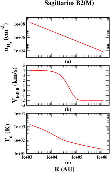
Figure 27: Spatial distribution of physical parameters: (a) H₂ density, (b) In-fall velocity, and (c) Dust temperatures for hot corino (IRAS4A) and hot core (Sagittarius B2) are taken from Mottram et al. (2013) and Rolffs et al. (2010) respectively.

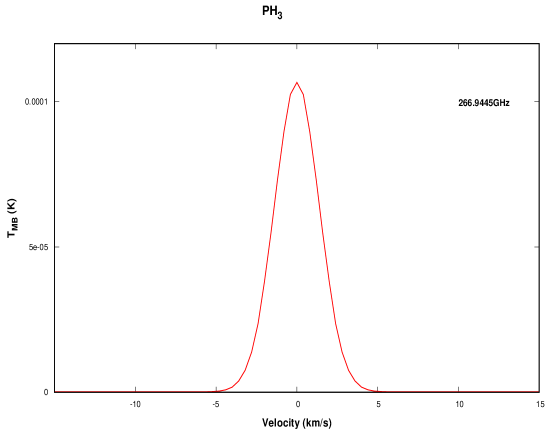
Figure 28: The line profile of the transition of PH₃, which could be observed with the IRAM-30m toward IRAS4A is shown with the RATRAN model. Abundance of PH₃ is taken from the CMMC model of hot corino noted in Table 6.

References

- Adams et al. (1990) Adams, N. G., McIntosh, B. J., & Smith, D. 1990, A&A, 232, 443
- Agúndez et al. (2014) Agúndez, M., Cernicharo, J., Decin, L., Encrenaz, P., & Teyssier, D. 2014, ApJ, 790, L27, doi: 10.1088/2041-8205/790/2/L27
- Agúndez et al. (2007) Agúndez, M., Cernicharo, J., & Guélin, M. 2007, ApJ, 662, L91, doi: 10.1086/519561
- Agúndez et al. (2008) Agúndez, M., Cernicharo, J., Pardo, J. R., Guélin, M., & Phillips, T. G. 2008, A&A, 485, L33, doi: 10.1051/0004-6361:200810193
- Altwegg et al. (2016) Altwegg, K., Balsiger, H., Bar-Nun, A., et al. 2016, Science Advances, 2, e1600285, doi: 10.1126/sciadv.1600285
- Anicich (1993) Anicich, V. G. 1993, ApJS, 84, 215, doi: 10.1086/191752
- Aota & Aikawa (2012) Aota, T., & Aikawa, Y. 2012, ApJ, 761, 74, doi: 10.1088/0004-637X/761/1/74
- Bains et al. (2020) Bains, W., Petkowski, J. J., Seager, S., et al. 2020, arXiv e-prints, arXiv:2009.06499. https://arxiv.org/abs/2009.06499
- Becke (1993) Becke, A. D. 1993, The Journal of Chemical Physics, 98, 5648, doi: 10.1063/1.464913
- Bergner et al. (2019) Bergner, J. B., Öberg, K. I., Walker, S., et al. 2019, ApJ, 884, L36, doi: 10.3847/2041-8213/ab48f9
- Bernal et al. (2021) Bernal, J. J., Koelemay, L. A., & Ziurys, L. M. 2021, ApJ, 906, 55, doi: 10.3847/1538-4357/abc87b
- Boogert et al. (2015) Boogert, A. C. A., Gerakines, P. A., & Whittet, D. C. B. 2015, ARA&A, 53, 541, doi: 10.1146/annurev-astro-082214-122348
- Bregman et al. (1975) Bregman, J., Lester, D., & Rank, D. 1975, The Astrophysical Journal, 202, L55
- Cancès et al. (1997) Cancès, E., Mennucci, B., & Tomasi, J. 1997, Journal of Chemical Physics, 107, 3032, doi: 10.1063/1.474659
- Caux et al. (2011) Caux, E., Kahane, C., Castets, A., et al. 2011, A&A, 532, A23, doi: 10.1051/0004-6361/201015399
- Chang et al. (2021) Chang, Q., Zheng, X.-L., Zhang, X., et al. 2021, Research in Astronomy and Astrophysics, 21, 039, doi: 10.1088/1674-4527/21/2/39
- Chantzos et al. (2020) Chantzos, J., Rivilla, V. M., Vasyunin, A., et al. 2020, A&A, 633, A54, doi: 10.1051/0004-6361/201936531
- Charnley & Millar (1994) Charnley, S. B., & Millar, T. J. 1994, Monthly Notices of the Royal Astronomical Society, 270, 570, doi: 10.1093/mnras/270.3.570
- Cheung et al. (1968) Cheung, A. C., Rank, D. M., Townes, C. H., Thornton, D. D., & Welch, W. J. 1968, Phys. Rev. Lett., 21, 1701, doi: 10.1103/PhysRevLett.21.1701
- Das et al. (2015) Das, A., Majumdar, L., Sahu, D., et al. 2015, ApJ, 808, 21, doi: 10.1088/0004-637X/808/1/21
- Das et al. (2018) Das, A., Sil, M., Gorai, P., Chakrabarti, S. i. K., & Loison, J. C. 2018, ApJS, 237, 9, doi: 10.3847/1538-4365/aac886
- De Beck et al. (2013) De Beck, E., Kamiński, T., Patel, N. A., et al. 2013, A&A, 558, A132, doi: 10.1051/0004-6361/201321349
- Draine (1978) Draine, B. T. 1978, ApJS, 36, 595, doi: 10.1086/190513
- Dubernet et al. (2013) Dubernet, M. L., Alexander, M. H., Ba, Y. A., et al. 2013, A&A, 553, A50, doi: 10.1051/0004-6361/201220630
- Dunning (1989) Dunning, Thom H., J. 1989, J. Chem. Phys., 90, 1007, doi: 10.1063/1.456153
- Ferland et al. (2017) Ferland, G. J., Chatzikos, M., Guzmán, F., et al. 2017, Rev. Mexicana Astron. Astrofis., 53, 385. https://arxiv.org/abs/1705.10877
- Ferrero et al. (2020) Ferrero, S., Zamirri, L., Ceccarelli, C., et al. 2020, ApJ, 904, 11, doi: 10.3847/1538-4357/abb953
- Fletcher et al. (2009) Fletcher, L. N., Orton, G. S., Teanby, N. A., & Irwin, P. G. J. 2009, Icarus, 202, 543, doi: 10.1016/j.icarus.2009.03.023
- Fontani et al. (2016) Fontani, F., Rivilla, V. M., Caselli, P., Vasyunin, A., & Palau, A. 2016, ApJ, 822, L30, doi: 10.3847/2041-8205/822/2/L30
- Fontani et al. (2019) Fontani, F., Rivilla, V. M., van der Tak, F. F. S., et al. 2019, MNRAS, 489, 4530, doi: 10.1093/mnras/stz2446
- Frisch et al. (2013) Frisch, M. J., Trucks, G. W., Schlegel, H. B., et al. 2013, Gaussian 09 Revision D.01
- Gorai et al. (2020) Gorai, P., Bhat, B., Sil, M., et al. 2020, ApJ, 895, 86, doi: 10.3847/1538-4357/ab8871
- Gorai et al. (2017a) Gorai, P., Das, A., Das, A., et al. 2017a, ApJ, 836, 70, doi: 10.3847/1538-4357/836/1/70
- Gorai et al. (2017b) Gorai, P., Das, A., Majumdar, L., et al. 2017b, Molecular Astrophysics, 6, 36, doi: 10.1016/j.molap.2017.01.004
- Gorai et al. (2020) Gorai, P., Sil, M., Das, A., et al. 2020, ACS Earth and Space Chemistry, 4, 920–946, doi: 10.1021/acsearthspacechem.0c00098
- Greaves et al. (2020) Greaves, J. S., Richards, A. M. S., Bains, W., et al. 2020, Nature Astronomy, doi: 10.1038/s41550-020-1174-4
- Guelin et al. (1990) Guelin, M., Cernicharo, J., Paubert, G., & Turner, B. E. 1990, A&A, 230, L9
- Halfen et al. (2008) Halfen, D. T., Clouthier, D. J., & Ziurys, L. M. 2008, ApJ, 677, L101, doi: 10.1086/588024
- Hincelin et al. (2015) Hincelin, U., Chang, Q., & Herbst, E. 2015, A&A, 574, A24, doi: 10.1051/0004-6361/201424807
- Hogerheijde & van der Tak (2000) Hogerheijde, M. R., & van der Tak, F. F. S. 2000, A&A, 362, 697. https://arxiv.org/abs/astro-ph/0008169
- Jarosewich (1990) Jarosewich, E. 1990, Meteoritics, 25, 323, doi: 10.1111/j.1945-5100.1990.tb00717.x
- Jenkins (2009) Jenkins, E. B. 2009, ApJ, 700, 1299, doi: 10.1088/0004-637X/700/2/1299