Evading Thermodynamic Uncertainty Relations via Asymmetric Dynamic Protocols

Abstract

Many versions of Thermodynamic Uncertainty Relations (TUR) have recently been discovered, which impose lower bounds on relative fluctuations of integrated currents in irreversible dissipative processes, and suggest that there may be fundamental limitations on the precision of small scale machines and heat engines. In this work we rigorously demonstrate that TUR can be evaded by using dynamic protocols that are asymmetric under time-reversal. We illustrate our results using a model heat engine using two-level systems, and also discuss heuristically the fundamental connections between TUR and time-reversal symmetry.

In recent years, several classes of inequalities have been discovered, which indicate trade-offs between various aspects of non-equilibrium processes. For example, many versions of thermodynamic uncertainty relations (TUR) Barato2015thermodynamic ; Horowitz-2019-NP-review ; Gingrich-2016 ; Pietzonka2016 ; Gingrich-2017 ; Koyuk-2019 ; Macieszczak-2018 ; Hasegawa-2019 ; Potts2019thermodynamic ; Proesmans2017 ; Gingrich-2016-prl ; proesmans2019hysteretic ; Shiraishi-2017 ; Horowitz2017 ; Timpanaro-2019 ; Seifert-2017 ; vo2020unified ; Pietzonka2018universal ; Pal2019experimental ; Friedman2020 ; Hasegawa2019quantum ; Dechant2019 footnote-TUR impose lower bounds of integrated current fluctuations in terms of entropy production, which signify a trade-off between dissipation and precision for small-scale machines. Another example is the so-called speed-limit inequalities Aurell-2011 ; Aurell-2012 ; Shiraishi-2016 ; Okuyama-2018 ; Shanahan-2018 ; Shiraishi-2018 ; Dechant-2019 ; Ito-2020 , which indicate a trade-off between efficiency and power output for general Markov processes. Most recently, Dechant and Sasa Dechant-2020 derived an upper bound for non-equilibrium response function in terms of fluctuations and relative entropy between the perturbed and reference states, which generated immediate interests Dechant-2020-1 ; Hasegawa2019quantum ; Dechant-2020-3 . Given the large number of works published in recent years, it is highly desirable and urgent to understand whether these inequalities are consequences of more fundamental aspects of non-equilibrium physics, such as Fluctuation Theorems and Markovian property, or rather depend on specific system details.

The current situation of TUR is particularly vibrant and complex Horowitz-2019-NP-review . The first version of TUR, which was proposed Barato2015thermodynamic and proved Gingrich-2016 for continuous time Markov jump processes with local detailed balance, has the form: ${\langle\delta Q^{2}\rangle}/{\langle Q\rangle^{2}}\geq{2}/{\langle\Sigma\rangle}$, where $Q$ is certain integrated current, and $\langle\Sigma\rangle$ the average entropy production. It was very quickly generalized to other types of irreversible processes, including finite-time processes Seifert-2017 ; Gingrich-2016-prl ; Dechant2019 ; Horowitz2017 discrete time processes Shiraishi-2017 ; Proesmans2017 , and most recently quantum processes Hasegawa2019quantum ; Friedman2020 . Its relation to the linear response theory has also been clarified Macieszczak-2018 . More recently, Timpanaro et. al.  Timpanaro-2019 and Hasegawa et. al. Hasegawa-2019 proved tighter TUR bounds in the form of ${\langle\delta Q^{2}\rangle}/{\langle Q\rangle^{2}}\geq f({\langle\Sigma\rangle})$ for general processes with symmetric dynamic protocols. For small $\langle\Sigma\rangle$, $f({\langle\Sigma\rangle})\sim 2/\langle\Sigma\rangle$, so that the original TUR is restored. For large $\langle\Sigma\rangle$, $f({\langle\Sigma\rangle})$ vanishes exponentially . These generalized TUR has their origin in Fluctuation Theorem Seifert-review ; Searles-1999 ; Crooks-1999 , and hence are universal and independent of model details. The deep connection between fluctuation of entropy production and Fluctuation Theorem was previously studied by Merhav and Kafri Merhav-2010 .

While almost all previous works concern processes with dynamic protocols that are symmetric under time-reversal, employment of asymmetric dynamic protocol provides another dimension for the issue of TUR. Results about asymmetric dynamic protocols are scarce, but did indicate a very different scenario. Barrato and Seifert Barato2016 showed that Brownian clock driven periodically can achieve arbitrary high precision with arbitrary low dissipation. Chun et. al.  Barato2019-magnetic showed that TUR may not work for system coupled to a magnetic field, which explicitly breaks the time-reversal symmetry. In light of these results, it is highly desirable to know whether in principle TUR-bound can always be evaded via clever design of asymmetric dynamic protocols. This question, which is independent of model details, is of fundamental importance for study of small scale machines Kay2010 ; Rayment1993 ; Balzani2000 ; Douglas2012 ; Requicha2003 ; Wang1998 ; Kolomelsky2007 .

In this letter, we shall rigorously establish the absence of TUR-bound for processes with asymmetric dynamic protocols. We shall minimize the relative current fluctuations with the constraints of (1) fixed entropy production and (2) satisfaction of Detailed Fluctuation Theorem, which is valid for processes with asymmetric protocols, and show that the lower bound for the current fluctuations is strictly zero. Hence all TUR-bounds can be evaded via clever designs of asymmetric dynamic protocols. To illustrate our results, we also discuss a model of heat engine whose output fluctuation can be tuned arbitrarily small. Finally we present a heuristic discussion in terms of Detailed Fluctuation Theorem why TUR-bounds exist in processes with symmetric dynamic protocols but not in those with asymmetric dynamic protocols. Our results provide important insights for design of high precision microscopic machines and heat engines.

Fluctuation Theorem  Consider an irreversible stochastical process with path probability distribution $P_{U}[\gamma]$, where $U=\{\lambda(t),t\in(0,T)\}$ denotes the dynamic protocol, and $\lambda(t)$ is the time-dependent external parameter, and $(0,T)$ is the time-range of the process. Associated with this process is the backward process, with a reversed protocol $\bar{U}=\{\bar{\lambda}(t)=\lambda^{*}(-t),t\in(-T,0)\}$ and a path probability distribution $P_{\bar{U}}[\gamma]$. Note that $\lambda^{*}$ is related to $\lambda$ via reversal of odd parameters, such as magnetic field. Assuming that there is separation of time-scale, and that all slow variables included in the model, the entropy production $\Sigma[\gamma]$ of the forward process along the path $\gamma$ satisfies Maes2003time ; seifert2005entropy

$${P_{U}[\gamma]}={P_{\bar{U}}[\bar{\gamma}]}\,e^{\Sigma[\gamma]},$$ (1)

which automatically implies $\Sigma[\gamma]=-\bar{\Sigma}[\bar{\gamma}]$, i.e., entropy production changes sign under the reversal of both the path and the dynamic protocol. Here $\bar{\gamma}$ is the time-reversal of the path forward $\gamma$, which is obtained from $\gamma$ via reversal of both time and odd variables. Equation (1) has been established for classical systems on very general ground Maes2003time ; seifert2005entropy . It is also known to hold for certain quantum systems Campisi-RMP-2011-QFT . We shall be interested in asymmetric protocols i.e., $U\neq\bar{U}$, which means that the forward and backward processes are macroscopically different.

Now consider a certain integrated current $Q[\gamma]$ as a functional of path, which is odd under time-reversal, i.e., $\bar{Q}[\bar{\gamma}]=-Q[\gamma]$. It may be the amount of matter transported or heat conducted along the path $\gamma$. The joint probability density functions (pdf) of $\Sigma[\gamma]$ and $Q[\gamma]$ for the forward and backward processes are

$$p(\sigma,q) = \sum_{\gamma}p_{U}[\gamma]\,\delta(\sigma-\Sigma[\gamma])\delta(q-Q[\gamma]),$$ (2)

$$\bar{p}(\sigma,q) = \sum_{\gamma}p_{\bar{U}}[\gamma]\,\delta(\sigma-\bar{\Sigma}[\gamma])\delta(q-\bar{Q}[\gamma]).$$ (3)

Generalizing a theorem due to van der Broeck and Cleuren Broeck-Cleuren-comment-2007 , we can readily obtain a generalized version of Detailed Fluctuation Theorem (DFT):

$$p(\sigma,q)=\bar{p}(-\sigma,-q)\,e^{\sigma}.$$ (4)

All statistical properties of $\Sigma$ and $Q$ for the forward and backward processes can be obtained from $p(\sigma,q)$ and $\bar{p}(\sigma,q)$. If the dynamic protocol is symmetric, $\bar{U}=U$ and $\bar{p}=p$, and Eq. (4) reduces to:

$$p(\sigma,q)={p}(-\sigma,-q)\,e^{\sigma},$$ (5)

which was the starting point of studies in Ref. Timpanaro-2019 ; Hasegawa-2019 . Our aim is to minimize the variances $\langle\delta Q^{2}\rangle$ and $\langle\delta\Sigma^{2}\rangle$ under the constraint of fixed averages $\langle\Sigma\rangle$ and $\langle Q\rangle$, for all distributions that satisfying Eq. (4).

Minimization of Fluctuations   In this section we will show that DFT (4) implies no TUR bound for fluctuations. Any continuous probability distribution can be approximated, to an arbitrary precision, by a discrete distribution. Hence we only need to study discrete distributions. We shall use the term N-point distribution to denote a probability distribution in the form of $p_{N}(\sigma,q)=\sum_{i}^{N}p_{i}\delta(\sigma-\sigma_{i})\delta(q-q_{i})$. Let $\{p_{N}(\sigma,q),\bar{p}_{N}(-\sigma,-q)\}$ be a pair of $N$-point distributions for the forward and backward processes satisfying Eq. (4). As shown in detail in Supplementary Informations (SI), for any $N\geq 3$, we can always construct a pair of $(N-1)$-point distributions $\{p_{N-1}(\sigma,q),\bar{p}_{N-1}(-\sigma,-q)\}$ which also satisfy Eq. (4) but has equal averages $\langle\Sigma\rangle$ and $\langle Q\rangle$ and smaller fluctuations $\langle\delta Q^{2}\rangle$ and $\langle\delta\Sigma^{2}\rangle$. Repeating this process, we eventually arrive at the following lemma:

Lemma 1

For any pair of N-point distributions $p_{N}(\sigma,q),\bar{p}_{N}(\sigma,q)$ obeying DFT Eq. (4), we can always find a pair of 2-point distributions $p_{2}(\sigma,q),\bar{p}_{2}(\sigma,q)$ such that, comparing with $p_{N}(\sigma,q)$, $p_{2}(\sigma,q)$ has same averages $\langle\Sigma\rangle,\langle Q\rangle$ and smaller variances $\langle\delta\Sigma^{2}\rangle$ and $\langle\delta Q^{2}\rangle$.

The detailed proof of this lemma is shown in SI.

Let us further try to find the pair $p_{2}(\sigma,q),\bar{p}_{2}(\sigma,q)$ that produces the minimal fluctuations $\langle\delta\Sigma^{2}\rangle$ and $\langle\delta Q^{2}\rangle$. We shall first treat the simple case $Q=\Sigma$, so that we only need to minimize $\langle\delta\Sigma^{2}\rangle$ with fixed $\langle\Sigma\rangle$. Let us write:

$$p_{2}(\sigma) = p\,\delta(\sigma-\sigma_{1})+(1-p)\,\delta(\sigma-\sigma_{2}),$$ (6a)

$$\bar{p}_{2}(\sigma) = p\,e^{-\sigma_{1}}\,\delta(\sigma+\sigma_{1})+(1-p)\,e^{-\sigma_{2}}\,\delta(\sigma-\sigma_{2}),\quad\,\,$$ (6b)

which satisfy Eq. (4). Whereas $$p(\sigma) \bar{p}(\sigma) p \sigma_{1},\sigma_{2}$$ is already normalized, normalization of fixes in terms of :

$$p=\frac{1-e^{-\sigma_{2}}}{e^{-\sigma_{1}}-e^{-\sigma_{2}}}.$$ (6c)

Using Eqs. (6) we find averages and fluctuations of $\Sigma$ for the forward and backward processes:

$$\langle\Sigma\rangle = \frac{\sigma_{2}(e^{-\sigma_{1}}-1)+\sigma_{1}(1-e^{-\sigma_{2}})}{e^{-\sigma_{1}}-e^{-\sigma_{2}}},$$ (7a)

$$\langle\delta\Sigma^{2}\rangle = \frac{(\sigma_{1}-\sigma_{2})^{2}(e^{-\sigma_{1}}-1)(1-e^{-\sigma_{2}})}{(e^{-\sigma_{1}}-e^{-\sigma_{2}})^{2}},$$ (7b)

$$\overline{\langle\Sigma\rangle} = \frac{-\sigma_{1}e^{-\sigma_{1}}(1-e^{-\sigma_{2}})-\sigma_{2}e^{-\sigma_{2}}(e^{-\sigma_{1}}-1)}{e^{-\sigma_{1}}-e^{-\sigma_{2}}},\quad$$ (7c)

$$\overline{\langle\delta\Sigma^{2}\rangle} = \frac{(\sigma_{1}-\sigma_{2})^{2}(e^{\sigma_{2}}-1)(1-e^{\sigma_{1}})}{(e^{\sigma_{1}}-e^{\sigma_{2}})^{2}}.$$ (7d)

If $\sigma_{1}=0$ ($\sigma_{2}=0$), $p=1$ ($p=0$), the entropy production is always zero, which corresponds to a reversible process. This is not what we aim to study in this work, hence we shall assume that neither of $\sigma_{1},\sigma_{2}$ vanish. From Eq. (6c) we see to make $p$ or $1-p$ both positive, $\sigma_{1},\sigma_{2}$ must have different signs. Let us assume $\sigma_{1}<0<\sigma_{2}$.

Let us now fix $\sigma_{2}>0$, and make $|\sigma_{1}|=-\sigma_{1}\gg 1$, hence $e^{-\sigma_{1}}\gg 1$, and $p\sim e^{\sigma_{1}}=e^{-|\sigma_{1}|}\ll 1$, according to Eq. (6c). From Eqs. (7) we obtain the following asymptotics:

$$\langle\Sigma\rangle \sim \sigma_{2},$$ (8a)

$$\langle\delta\Sigma^{2}\rangle \sim \sigma_{1}^{2}(1-e^{-\sigma_{2}})e^{\sigma_{1}}\rightarrow 0,$$ (8b)

$${\langle\delta\Sigma^{2}\rangle}/{\langle\Sigma\rangle^{2}} \sim \sigma_{2}^{-2}\sigma_{1}^{2}(1-e^{-\sigma_{2}})e^{\sigma_{1}}\rightarrow 0.\quad\quad$$ (8c)

Hence in the forward process, $$\langle\Sigma\rangle \langle\delta\Sigma^{2}\rangle \sigma_{1}$$ converges to a finite limit, whereas becomes exponentially small in . Similarly for the backward process we obtain

$$\overline{\langle\Sigma\rangle} \sim -\sigma_{1}+\sigma_{1}e^{-\sigma_{2}}\rightarrow\infty,$$ (8d)

$$\overline{\langle\delta\Sigma^{2}\rangle} \sim \sigma_{1}^{2}e^{-2\sigma_{2}}(e^{\sigma_{2}}-1)\rightarrow\infty,$$ (8e)

$$\overline{\langle\delta\Sigma^{2}\rangle}/\overline{\langle\Sigma\rangle}^{2} \sim {1}/{(e^{\sigma_{2}}-1)}.$$ (8f)

Hence in the backward process, both $\langle\Sigma\rangle$ and $\langle\delta\Sigma^{2}\rangle$ diverge, whereas $\overline{\langle\delta\Sigma^{2}\rangle}/\overline{\langle\Sigma\rangle}^{2}$ converges to a finite limit.

Let us now consider the general case where $Q$ is an integrated current distinct from entropy production. The joint distributions of $\Sigma$ and $Q$ have the following forms:

$$p_{2}(\sigma,q) = p\,\delta(\sigma-\sigma_{1})\delta(q-q_{1})$$ (9a)

$$+ (1-p)\,\delta(\sigma-\sigma_{2})\delta(q-q_{2}),$$

$$\bar{p}_{2}(\sigma,q) = p\,e^{-\sigma_{1}}\,\delta(\sigma+\sigma_{1})\delta(q+q_{1})$$ (9b)

$$+ (1-p)\,e^{-\sigma_{2}}\,\delta(\sigma+\sigma_{2})\delta(q+q_{2}),\quad$$

where $p$ is still given by Eq. (6c). Whilst the average entropy productions are still given by Eqs. (7), the average and variance of $Q$ can be calculated using Eqs. (9). Recall that we fix $\sigma_{2}>0$ and let $\sigma_{1}\rightarrow-\infty$. In this limit, we have for the forward process:

$$\langle\delta Q^{2}\rangle \sim {(q_{1}-q_{2})^{2}e^{\sigma_{1}}(1-e^{-\sigma_{2}})},$$ (10a)

$$\langle Q\rangle \sim q_{2}.$$ (10b)

For all reasonable physical models, we expect that entropy production scales quadratically (or at least polynomially) with the current. Hence $$q_{1} \sigma_{1} q_{2} \langle\delta Q^{2}\rangle \langle Q\rangle Q$$ diverges with , whereas remains finite. From Eqs. (10) we find that converges to zero, whereas remains fixed. The relative fluctuation of converges to zero:

$$\langle\delta Q^{2}\rangle/\langle Q\rangle^{2}\sim q_{2}^{-2}q_{1}^{2}(1-e^{-\sigma_{2}})e^{\sigma_{1}}\rightarrow 0.$$ (10c)

For the backward process we have

$$\overline{\langle\delta Q^{2}\rangle} \sim {(q_{1}-q_{2})^{2}e^{-\sigma_{2}}(1-e^{-\sigma_{2}})},$$ (10d)

$$\overline{\langle Q\rangle} \sim -(1-e^{-\sigma_{2}})q_{1}-e^{-\sigma_{2}}q_{2}.$$ (10e)

hence both $$\overline{\langle\delta Q^{2}\rangle} \overline{\langle Q\rangle} q_{1} Q$$ and diverge with . The relative fluctuation of converges to the same limit as in Eq. (8f):

$$\overline{\langle\delta Q^{2}\rangle}/\overline{\langle Q\rangle}^{2}\sim{1}/{(e^{\sigma_{2}}-1)},$$ (10f)

Naturally one may wonder whether it is possible to make current fluctuations small for both the forward and backward process. This is impossible. In Refs. Potts2019thermodynamic ; proesmans2019hysteretic the following inequality was derived from DFT (4):

$$\frac{\langle\delta Q^{2}\rangle+\overline{\langle\delta Q^{2}\rangle}}{(\langle Q\rangle+\overline{\langle Q\rangle})^{2}}\geq{{\rm exp}-\frac{1}{2}\left[\langle\Sigma\rangle+\overline{\langle\Sigma\rangle}\right]}.$$ (11)

If $\langle Q\rangle,\overline{\langle Q\rangle}$, $\langle\Sigma\rangle,\overline{\langle\Sigma\rangle}$ are all finite, and $\langle\delta Q^{2}\rangle,\overline{\langle\delta Q^{2}\rangle}$ are very small, Eq. (11) must be violated. On the other hand, for the two-point distributions we studied above, using Eqs. (10), we see that the LHS of Eq. (11) converges to ${1}/{(e^{\sigma_{2}}-1)}>0$, whereas RHS of Eq. (11) converges to zero. Hence the inequality (11) is not tight.

These results show unambiguously that there is no TUR bound for entropy production as long as asymmetric dynamic protocols are allowed. In Ref. Brandner-2018 , Brandner et. al. studied an irreversible process with magnetic field and certain dynamic protocol, and discovered a non-vanishing TUR bound for current fluctuations. This does not contradict our theory. Instead our theory means that the TUR bound discovered in Ref. Brandner-2018 can be evaded if more sophisticated protocols are used.

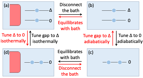
Figure 1: Schematics of the qubit model. The red regions denote heat baths. Black arrows and red arrows denote respectively forward and backward dynamic protocols. Two energy levels are degenerate in (c) and (d).

A model heat engine   We shall now discuss a concrete irreversible process with finite $\langle\Sigma\rangle$ and vanishingly small current fluctuations. Consider a two-level system with a Hamiltonian

$$\hat{H}(\Delta)=\Delta\,\begin{pmatrix}1&0\\ 0&0\end{pmatrix},\quad\Delta>0,$$ (12)

where the energy of the excited state $\Delta$ that can be tuned externally. We shall construct an irreversible cycle that starts from a Gibbs state $\hat{\rho}(\Delta)=Z^{-1}e^{-\beta\hat{H}(\Delta)}$, illustrated by panel (a) of Fig. 1 (top left), which can be obtained by connecting the system to a heat bath with temperature $T=1/\beta$. As illustrated by the black arrows in Fig. 1, the cycle consists of the following four steps $(a)\stackrel{{\scriptstyle\tiny 1}}{{\rightarrow}}(b)\stackrel{{\scriptstyle\tiny 2}}{{\rightarrow}}(c)\stackrel{{\scriptstyle\tiny 3}}{{\rightarrow}}(d)\stackrel{{\scriptstyle\tiny 4}}{{\rightarrow}}(a)$:

1. Disconnection of the system from the heat bath.

2. Adiabatic process: We adiabatically tune the parameter $\Delta$ to $0$, during which the system remains in the state $\hat{\rho}=Z^{-1}e^{-\beta\hat{H}(\Delta)}$.

3. Equilibration process: We reconnect the system to the bath, and the system re-equilibrates to a new Gibbs state $\hat{\rho}=Z^{-1}e^{-\beta\hat{H}(0)}=\hat{\bm{I}}/2$. This step is irreversible process with an entropy increase.

4. Isothermal process: With the system connected to the bath, the gap is tuned isotatically back to $\Delta$ so that the density matrix returns to the initial state $\hat{\rho}(\Delta)=Z^{-1}e^{-\beta\hat{H}(\Delta)}$.

In stages (a) and (d), the system is in the relevant Gibbs-Boltzmann state. In stages (b) and (c), the system is either at the excited level (with probability $p=e^{-\beta\Delta}/(1+e^{-\beta\Delta})$) or at the ground level (with probability $1-p=1/(1+e^{-\beta\Delta})$). There are two paths for the adiabatic process, $\gamma_{1}=\{{\rm Gibbs}\rightarrow{\rm excited}\rightarrow{\rm excited}\rightarrow{\rm Gibbs}\}$ with probabilities $p$, and $\gamma_{2}=\{{\rm Gibbs}\rightarrow{\rm ground}\rightarrow{\rm ground}\rightarrow{\rm Gibbs}\}$, with probabilities $1-p$. These two paths merge in stages (a) and (d).

The only integrated current in this problem is the entropy production. Since the process is cyclic, the entropy production is related to the work done by the external force via $\Sigma=\beta W$. Let us consider the adiabatic process. Along the path $\gamma_{1}$, the system remains in the excited state, and the external force does work $-\Delta$. Along the path $\gamma_{2}$, the work is identically zero. During the isothermal process, two path coincide, and the work done equals to the change of system free energy, which is $T\log{2}/({1+e^{-\beta\Delta}})$. Hence the total works along two paths are respectively:

$$W[\gamma_{1}] = -\Delta+T\log\frac{2}{1+e^{-\beta\Delta}}=T\log(2p),$$ (13a)

$$W[\gamma_{2}] = T\log\frac{2}{1+e^{-\beta\Delta}}=T\log 2(1-p).$$ (13b)

Hence the path probabilities and the entropy production of $\gamma_{1},\gamma_{2}$ are respectively

$$p_{1}=p=\frac{e^{-\beta\Delta}}{1+e^{-\beta\Delta}},\quad p_{2}=1-p,$$ (14a)

$$\sigma_{1}=\log(2p),\quad\sigma_{2}=\log 2(1-p).$$ (14b)

This is a special case of Eqs. (6), with only one independent parameter $$p \beta\Delta$$ (or equivalently ).

The backward process is obtained by reversing the dynamic protocols, shown as all red arrows in Fig. 1. In the backward process, the system starts from the equilibrium state $\hat{\rho}=Z^{-1}e^{-\beta\hat{H}(\Delta)}$ (a), and goes through consecutively isothermal, disconnection, and adiabatic, and connection steps . The two paths diverge from each other during the adiabatic process (c) $\rightarrow$ (b). In the stage (c), two levels are degenerate, and the system is in each of them with probability $1/2$. The works done by the external force during each path in the backward process are the negative of those in the forward process. Hence we have for the backward process:

$$\bar{p}_{1}=\frac{1}{2},\quad\bar{p}_{2}=\frac{1}{2},$$ (14c)

$$\bar{\sigma}_{1}=-\log(2p),\quad\bar{\sigma}_{2}=-\log 2(1-p).$$ (14d)

We easily verify that Eqs. (14) satisfy the entropy production formula, Eq. (1).

As we make $\beta\Delta$ large, $p\rightarrow 0$, and $\sigma_{1}\rightarrow 0$, $\sigma_{2}\rightarrow\log 2$, and we recover all the asymptotics in Eqs. (8). More concretely, in the forward process, $\langle\Sigma\rangle\rightarrow\log 2$, and $\langle\delta\Sigma^{2}\rangle\sim(\beta\Delta)^{2}e^{-\beta\Delta}\rightarrow 0$, whereas in the backward process, we have $\overline{\langle\Sigma\rangle}\rightarrow\beta\Delta/2$, and $\overline{\langle\delta\Sigma^{2}\rangle}\sim(\beta\Delta)^{2}/2$. The relative fluctuation of entropy production of the backward process converges to a finite limit $\overline{\langle\delta\Sigma^{2}\rangle}/\overline{\langle\Sigma\rangle}^{2}\rightarrow 2$.

Figure 2: A cartoon of pdf $p(\sigma,q)$ for processes with symmetric dynamic protocol. The high peak in the right is centered at $(q_{0},\sigma_{0})$, whereas the mirror peak in the left, which is dictated by the Detailed Fluctuation Theorem, is located at $(-q_{0},-\sigma_{0})$. The mirror peak can be diminished by using asymmetric dynamic protocols, thereby evading TUR bounds.

Heuristic discussion  We conclude our work with a heuristic discussion about TUR bounds in general irreversible processes. We aim, via tuning of dynamic protocols, to reduce the fluctuations of $\Sigma$ and $Q$, with their averages fixed and finite. The distribution $p(\sigma,q)$ then should have significant values only near a single point $(\sigma_{0},q_{0})$. Everywhere else $p(\sigma,q)$ must be negligibly small. However, if the dynamic protocol is symmetric under time-reversal, Eq. (5) must be respected, according to which there is a peak at the mirror point $(-\sigma_{0},-q_{0})$, as illustrated in Fig. 2. Equation (5) also dictates that the probabilities of the peak and of the mirror peak are respectively $1/(1+e^{-\sigma_{0}})$ and $1/(1+e^{\sigma_{0}})$. Using these probabilities one easily obtain $\langle\Sigma\rangle=\sigma_{0}\tanh(\sigma_{0}/2)$ and $\langle\delta Q^{2}\rangle/\langle Q\rangle^{2}=2\,{\rm csch}^{2}(\sigma_{0}/2)$. The latter is in fact exactly the sharp TUR bound obtained recently by Timpanaro et. al. Timpanaro-2019 . For processes with asymmetric dynamic protocols, however, the relevant Detailed Fluctuation Theorem is Eq. (4) rather than Eq. (5). But Eq. (4) does not imposes any constraint on $p(\sigma,q)$. Instead, it determines $\bar{p}(\sigma,q)$ in terms of $p(\sigma,q)$. Hence by using asymmetric protocols, the mirror peak can be arbitrarily diminished, and the TUR bound can be evaded, with average entropy production finite. Note that this heuristic discussion is applicable to models with continuous distributions of dynamic paths as well.

Acknowledgement X.X. acknowledges support from NSFC via grant #11674217, as well as additional support from a Shanghai Talent Program. This research is also supported by Shanghai Municipal Science and Technology Major Project (Grant No.2019SHZDZX01).

Supplementary Informations

Proof of Lemma 1

Let us write down a pair of N-point probability distributions, which satisfy the Detailed Fluctuation Theorem (4):

$$p_{N}(\sigma,q) = \sum_{i=1}^{N}p_{i}\,\delta(\sigma-\sigma_{i})\delta(q-q_{i}),$$ (15a)

$$\bar{p}_{N}(\sigma,q) = \sum_{i=1}^{N}p_{i}\,e^{-\sigma_{i}}\,\delta(\sigma+\sigma_{i})\delta(q+q_{i}).$$ (15b)

Normalization of two probability distributions require:

$$\sum_{i=1}^{N}p_{i} = 1,$$ (16a)

$$\sum_{i=1}^{N}p_{i}\,e^{-\sigma_{i}} = 1.$$ (16b)

Let $\sigma_{1}$ and $\sigma_{2}$ be the smallest and biggest of $\{\sigma_{i},i=1,\cdots,N\}$, and let us choose another point $\sigma_{3}$ such that $\sigma_{1}<\sigma_{3}<\sigma_{2}$. (If two or all of $\sigma_{1},\sigma_{2},\sigma_{3}$ are equal, we can tune $\sigma_{1},\sigma_{2},\sigma_{3}$ as well as $p_{1},p_{2},p_{3}$ such that $\sigma_{1}<\sigma_{3}<\sigma_{2}$ and at the same time the normalization conditions (16) remain valid, and $\langle\Sigma\rangle$ and $\langle Q\rangle$ remain fixed. This is always possible since we have six parameters to satisfy four independent constraints. Furthermore by choosing the direction of variation, we can always make sure that the variances of $\Sigma$ and $Q$ do not increase.) Now let us write down $\langle\Sigma\rangle,\langle\Sigma^{2}\rangle,\langle Q\rangle,\langle Q^{2}\rangle$:

$$\langle Q\rangle = p_{1}q_{1}+p_{2}q_{2}+p_{3}q_{3}+\sum_{i>3}p_{i}q_{i},$$ (17)

$$\langle Q^{2}\rangle = p_{1}q_{1}^{2}+p_{2}q_{2}^{2}+p_{3}q_{3}^{2}+\sum_{i>3}p_{i}q_{i}^{2},$$ (18)

$$\langle\Sigma\rangle = p_{1}\sigma_{1}+p_{2}\sigma_{2}+p_{3}\sigma_{3}+\sum_{i>3}p_{i}\sigma_{i},$$ (19)

$$\langle\Sigma^{2}\rangle = p_{1}\sigma_{1}^{2}+p_{2}\sigma_{2}^{2}+p_{3}\sigma_{3}^{2}+\sum_{i>3}p_{i}\sigma_{i}^{2}.$$ (20)

We shall redistribute infinitesimally the probability $p_{3}$ to $p_{1},p_{2}$, and at the same time tune $\sigma_{3}$ such that (a) Eqs. (16) remain valid, and (b) $\langle\Sigma\rangle$ remains invariant. Let us consider the infinitesimal transformation:

$$p_{i}\rightarrow p_{i}+dp_{i},\quad i=1,2,3,$$ (21)

$$\sigma_{3}\rightarrow\sigma_{3}+d\sigma_{3},$$ (22)

whereas all other $p_{k},\sigma_{k}$ remain invariant. Let us take the differential of Eqs. (16) and (19):

$$dp_{1}+dp_{2}+dp_{3} = 0,$$ (23)

$$e^{-\sigma_{1}}dp_{1}+e^{-\sigma_{2}}dp_{2}+e^{-\sigma_{3}}dp_{3}-e^{-\sigma_{3}}p_{3}d\sigma_{3} = 0,\quad$$ (24)

$$d\langle\Sigma\rangle=\sigma_{1}dp_{1}+\sigma_{2}dp_{2}+\sigma_{3}dp_{3}+p_{3}d\sigma_{3} = 0.\quad$$ (25)

Using these equations we can express $dp_{2},dp_{3},d\sigma_{3}$ in terms of $dp_{1}$. In particular we have

$$dp_{2}=-\frac{f(\sigma_{3}-\sigma_{1})}{f(\sigma_{3}-\sigma_{2})}dp_{1},$$ (26)

where $f(x)$ is a concave function with positive second derivative:

$$f(x)=e^{x}-1-x.$$ (27)

As illustrated in Fig. 3, $f(x)$ is non-negative and achieves minimum $f=0$ at $x=0$. Hence $dp_{2}$ and $dp_{1}$ always have different signs, since $\sigma_{1}<\sigma_{3}<\sigma_{2}$.

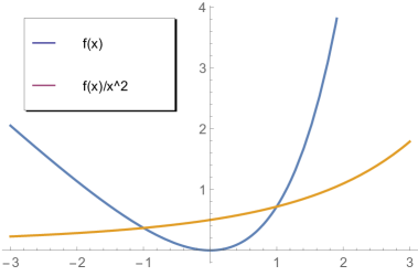
Figure 3: Plots of functions $f(x)=e^{x}-1-x$ and $f(x)/x^{2}$.

We can then calculate the differential of $\langle\Sigma^{2}\rangle$ and express in terms of $dp_{1}$:

$$d\langle\Sigma^{2}\rangle = \frac{(\sigma_{3}-\sigma_{1})^{2}(\sigma_{3}-\sigma_{2})^{2}}{f(\sigma_{3}-\sigma_{2})}$$ (28)

$$\times \left[\frac{f(\sigma_{3}-\sigma_{2})}{(\sigma_{3}-\sigma_{2})^{2}}-\frac{f(\sigma_{3}-\sigma_{1})}{(\sigma_{3}-\sigma_{1})^{2}}\right]dp_{1}.$$

As illustrated in Fig. 3, the function $f(x)/x^{2}$ is strictly monotonically increasing. Since $\sigma_{3}-\sigma_{2}<0$ and $\sigma_{3}-\sigma_{1}>0$, the difference in the bracket in the RHS of Eq. (28) is strictly negative. We shall chose $dp_{1}>0$, then we have $dp_{2}<0$, and $d\langle\Sigma^{2}\rangle<0$, and hence the variance $\langle\delta\Sigma^{2}\rangle$ decreases.

Let us now take care of the other variable $Q$. Let us take the differential of Eq. (17) and set it to zero:

$$d\,\langle Q\rangle=\sum_{i=1}^{3}p_{i}dq_{i}+\sum_{i=1}^{3}q_{i}dp_{i}=0.$$ (29)

With $dp_{2},dp_{3}$ determined previously in terms of $dp_{1}$, this equation defines a plane in the three dimensional space spanned by $dq_{1},dq_{2},dq_{3}$. Now let us take the differential of Eq. (18) and set it to zero:

$$d\langle Q^{2}\rangle=\sum_{i}2p_{i}q_{i}dq_{i}+\sum_{i}q_{i}^{2}dp_{i}=0,$$ (30)

which defines another plane in the same space. Assuming $q_{1},q_{2},q_{3}$ are not all identical, (If this condition is not satisfied, we can adjust $q_{1},q_{2},q_{3}$ such that they become different, whilst $\langle Q\rangle$ remains fixed.) these two planes are not parallel, and hence intersect each other on a straight line, which divided the plane Eq. (30) into two halves. As illustrated in Fig. 4, in one half, $d\langle Q^{2}\rangle$ is positive, whereas in the other half, $d\langle Q^{2}\rangle$ is negative. All we need is to pick an arbitrary point $(dq_{1},dq_{2},dq_{3})$ in the negative half plane, such that $d\langle Q^{2}\rangle$ is negative.

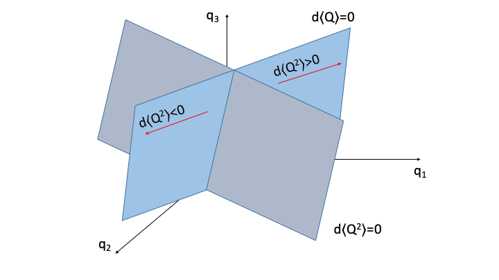
Figure 4: Illustration of the redistribution process to reduce the variance of Q.

Constructed as above, the redistribution process tunes the parameters $p_{1},p_{2},p_{3},\sigma_{3},q_{1},q_{2},q_{3}$ such that (i) Eq. (4) and the normalization conditions (16) remain valid, (ii) $p_{1}$ increases whereas $p_{2}$ decreases, (iii) the averages $\langle\Sigma\rangle$ and $\langle Q\rangle$ remain fixed, (iv) the variances $\langle\delta\Sigma^{2}\rangle$ and $\langle\delta Q^{2}\rangle$ decrease. Doing this iteratively either $p_{2}$ or $p_{3}$ will eventually become zero, and we can remove the point from the support of $p_{N}(\sigma,q)$ (and also remove the dual point from the support of $\bar{p}_{N}(\sigma,q)$). As a consequence we obtain a pair of $(N-1)$-point distributions $p_{N-1}(\sigma,q),\bar{p}_{N-1}(\sigma,q)$, such that $p_{N-1}(\sigma,q)$ has the same averages $\langle\Sigma\rangle$ and $\langle Q\rangle$, but smaller variances $\langle\delta\Sigma^{2}\rangle$ and $\langle\delta Q^{2}\rangle$ comparing to $p_{N}(\sigma,q)$. Keep doing this, we eventually obtain a pair of 2-point distributions $p_{2}(\sigma,q),\bar{p}_{2}(\sigma,q)$, such that $p_{2}(\sigma,q)$ has the same averages $\langle\Sigma\rangle$ and $\langle Q\rangle$, but smaller variances $\langle\delta\Sigma^{2}\rangle$ and $\langle\delta Q^{2}\rangle$ comparing to original distribution $p_{N}(\sigma,q)$.

References

- (1) Barato, Andre C. and Seifert, Udo. Thermodynamic Uncertainty Relation for Biomolecular Processes. Physical Review Letters 114.15 (2015).
- (2) Gingrich, Todd R., et al. Dissipation bounds all steady-state current fluctuations. Physical review letters 116.12 (2016): 120601.
- (3) Pietzonka, Patrick, Andre C. Barato, and Udo Seifert. Universal bound on the efficiency of molecular motors. Journal of Statistical Mechanics: Theory and Experiment 2016.12 (2016): 124004.
- (4) T. R. Gingrich, G. M. Rotskoff, and J. M. Horowitz, Inferring dissipation from current fluctuations, J. Phys. A: Math. Theor. 50, 184004 (2017).
- (5) Horowitz, Jordan M., and Todd R. Gingrich. Thermodynamic uncertainty relations constrain non-equilibrium fluctuations. Nature Physics (2019): 1-6.
- (6) AM Timpanaro, G Guarnieri, J Goold, and GT Landi. Thermodynamic uncertainty relations from exchange fluctuation theorems. Physical review letters 123 (2019): 090604.
- (7) Hasegawa, Yoshihiko, and Tan Van Vu. Fluctuation theorem uncertainty relation. Physical Review Letters 123.11 (2019): 110602.
- (8) Potts, Patrick P., and Peter Samuelsson. Thermodynamic uncertainty relations including measurement and feedback. Physical Review E 100.5 (2019).
- (9) Proesmans, Karel, and Jordan M. Horowitz. Hysteretic thermodynamic uncertainty relation for systems with broken time-reversal symmetry. Journal of Statistical Mechanics: Theory and Experiment 2019.5 (2019).
- (10) Van Tuan Vo and Tan Van Vu and Yoshihiko Hasegawa, Unified Approach to Classical Speed Limit and Thermodynamic Uncertainty Relation , arXiv:cond-mat.stat-mech 2007.03495(2020)
- (11) T. R. Gingrich, J. M. Horowitz, N. Perunov, and J. L. England, Physical Review letters 116, 120601 (2016).
- (12) Pal, Soham, et al. Experimental study of the thermodynamic uncertainty relation. arXiv: Statistical Mechanics (2019).
- (13) Friedman, Hava Meira, et al. ”Thermodynamic uncertainty relation in atomic-scale quantum conductors.” Physical Review B 101.19 (2020): 195423.
- (14) Patrick Pietzonka, Felix Ritort, and Udo Seifert. Finite-time generalization of the thermodynamic uncertainty relation. Phys. Rev. E 96, 012101 (2017).
- (15) J. M. Horowitz and T. R. Gingrich, Proof of the finite-time thermodynamic uncertainty relation for steady-state currents, Phys. Rev. E 96, 020103(R) (2017).
- (16) Pietzonka, Patrick, and Udo Seifert. Universal Trade-Off between Power, Efficiency, and Constancy in Steady-State Heat Engines. Physical Review Letters 120.19 (2018): 190602-190602.
- (17) Shiraishi, Naoto. Finite-time thermodynamic uncertainty relation do not hold for discrete-time Markov process. arXiv preprint arXiv:1706.00892 (2017).
- (18) K. Proesmans and C. Van den Broeck, Discrete-time thermodynamic uncertainty relation, EPL 119, 20001 (2017).
- (19) Macieszczak, Katarzyna, Kay Brandner, and Juan P. Garrahan. Unified thermodynamic uncertainty relations in linear response. Physical review letters 121.13 (2018): 130601.
- (20) Koyuk, Timur, and Udo Seifert. Operationally accessible bounds on fluctuations and entropy production in periodically driven systems. Physical review letters 122.23 (2019): 230601.
- (21) Hasegawa, Yoshihiko. ”Quantum thermodynamic uncertainty relation for continuous measurement.” Physical Review Letters 125 (2020): 050601.
- (22) Dechant, Andreas. Multidimensional thermodynamic uncertainty relations. Journal of Physics A 52.3 (2019).
- (23) Historically, the term thermodynamic uncertainty relation was first used to denote an inequality involving temperature and energy fluctuations Uffink-Van Lith-1999 in equilibrium thermal systems. Study of this topic goes back to Bohr and Heisenberg Bohr-Heisenberg-complementarity , who suspected a complementarity principle for classical thermodynamics analogous to that of quantum mechanics. These earlier works however are very different from the recent works which exclusively focus on irreversible processes with nonvanishing entropy production.
- (24) Aurell, Erik, Carlos Mejía-Monasterio, and Paolo Muratore-Ginanneschi. ”Optimal protocols and optimal transport in stochastic thermodynamics.” Physical review letters 106.25 (2011): 250601.
- (25) Aurell, Erik, et al. ”Refined second law of thermodynamics for fast random processes.” Journal of statistical physics 147.3 (2012): 487-505.
- (26) Shiraishi, Naoto, Keiji Saito, and Hal Tasaki. ”Universal trade-off relation between power and efficiency for heat engines.” Physical review letters 117.19 (2016): 190601.
- (27) Okuyama, Manaka, and Masayuki Ohzeki. ”Quantum speed limit is not quantum.” Physical review letters 120 (2018): 070402.
- (28) B Shanahan, A Chenu, N Margolus, and A Del Campo. ”Quantum speed limits across the quantum-to-classical transition.” Physical review letters 120 (2018): 070401.
- (29) Shiraishi, Naoto, Ken Funo, and Keiji Saito. ”Speed limit for classical stochastic processes.” Physical review letters 121 (2018): 070601.
- (30) Dechant, Andreas, and Yohei Sakurai. ”Thermodynamic interpretation of Wasserstein distance.” arXiv preprint arXiv:1912.08405 (2019).
- (31) Ito, Sosuke, and Andreas Dechant. ”Stochastic time evolution, information geometry, and the Cramér-Rao bound.” Physical Review X 10 (2020): 021056.
- (32) Dechant, Andreas, and Shin-ichi Sasa. Fluctuation–response inequality out of equilibrium. Proceedings of the National Academy of Sciences 117.12 (2020): 6430-6436.
- (33) Vo, Van Tuan, Tan Van Vu, and Yoshihiko Hasegawa. ”Unified Approach to Classical Speed Limit and Thermodynamic Uncertainty Relation.” arXiv preprint arXiv:2007.03495 (2020).
- (34) GrandPre, Trevor, et al. ”Entropy production fluctuations encode collective behavior in active matter.” arXiv preprint arXiv:2007.12149 (2020).
- (35) Seifert, Udo. “Stochastic thermodynamics, fluctuation theorems and molecular machines.” Reports on progress in physics 75.12 (2012): 126001.
- (36) Searles, Debra J., and Denis J. Evans. Fluctuation theorem for stochastic systems. Physical Review E 60 (1999): 159-164.
- (37) Crooks, G. E., 1999, Entropy production fluctuation theorem and the nonequilibrium work relation for free energy differences, Phys. Rev. E 60, 2721.
- (38) Merhav, Neri, and Yariv Kafri. Statistical properties of entropy production derived from fluctuation theorems. Journal of Statistical Mechanics: Theory and Experiment 2010.12 (2010): P12022.
- (39) Barato, A.C., and Udo Seifert. “Cost and Precision of Brownian Clocks”. Physical Review X 6 (2016), 041053.
- (40) Chun, Hyun-Myung and Fischer, Lukas P. and Seifert, Udo. Effect of a magnetic field on the thermodynamic uncertainty relation. Physical Review E 99 (2019): 042128.
- (41) Kay, Euan R., David A. Leigh, and Francesco Zerbetto. Synthetic molecular motors and mechanical machines. Angewandte Chemie International Edition 46.1-2 (2007):72-191.
- (42) Rayment, Ivan, et al. Three-dimensional structure of myosin subfragment-1: a molecular motor. Science 261.5117 (1993): 50-58.
- (43) Balzani, Vincenzo, et al. Artificial molecular machines. Angewandte Chemie International Edition 39.19 (2000): 3348-3391.
- (44) Douglas, Shawn M., Ido Bachelet, and George M. Church. A logic-gated nanorobot for targeted transport of molecular payloads. Science 335.6070 (2012): 831-834.
- (45) Requicha, Aristides AG. Nanorobots, NEMS, and nanoassembly. Proceedings of the IEEE 91.11 (2003): 1922-1933.
- (46) Wang, Hongyun, and George Oster. Energy transduction in the F 1 motor of ATP synthase. Nature 396.6708 (1998): 279-282.
- (47) A. B. Kolomeisky and M. E. Fisher, Molecular motors: A theorist’s perspective , Ann. Rev. Phys. Chem. 58 (2007) 675-695.
- (48) Uffink, Jos, and Janneke Van Lith. Thermodynamic uncertainty relations. Foundations of physics 29.5 (1999): 655-692.
- (49) N. Bohr, Collected Works, J. Kalckar, ed. (North-Holland, Amsterdam, 1985), Vol.6, pp. 316 - 330, 376 - 377.
- (50) Maes C, Netocny K. Time-reversal and entropy[J]. Journal of statistical physics, 2003, 110(1-2): 269-310.
- (51) Seifert U. Entropy production along a stochastic trajectory and an integral fluctuation theorem[J]. Physical review letters, 2005, 95: 040602.
- (52) Campisi, Michele, Peter Hänggi, and Peter Talkner. “Colloquium: Quantum fluctuation relations: Foundations and applications.” Reviews of Modern Physics 83.3 (2011): 771.
- (53) Van den Broeck, C., and B. Cleuren. Comment on “Irreversibility and Fluctuation Theorem in Stationary Time Series”. arXiv preprint cond-mat/0703213 (2007).
- (54) Brandner, Kay, Taro Hanazato, and Keiji Saito. ”Thermodynamic bounds on precision in ballistic multiterminal transport.” Physical review letters 120.9 (2018): 090601.