Enhancement of superconductivity by electronic nematicity in cuprate superconductors

Abstract

The cuprate superconductors are characterized by numerous ordering tendencies, with the electronically nematic order being the most distinct form of order. Here the intertwinement of the electronic nematicity with superconductivity in cuprate superconductors is studied based on the kinetic-energy-driven superconductivity. It is shown that the optimized $T_{\rm c}$ takes a dome-like shape with the weak and strong strength regions on each side of the optimal strength of the electronic nematicity, where the optimized $T_{\rm c}$ reaches its maximum. This dome-like shape nematic-order strength dependence of $T_{\rm c}$ thus indicates that the electronic nematicity enhances superconductivity. Moreover, this nematic order induces the anisotropy of the electron Fermi surface, where although the original electron Fermi surface contour with the four-fold rotation symmetry is broken up into that with a residual two-fold rotation symmetry, this electron Fermi surface contour with the two-fold rotation symmetry still is truncated to form the disconnected Fermi arcs with the most spectral weight that locates at around the tips of the Fermi arcs. Concomitantly, these tips of the Fermi arcs connected by the scattering wave vectors ${\bf q}_{i}$ construct an octet scattering model, however, the partial scattering wave vectors and their respective symmetry-corresponding partners occur with unequal amplitudes, leading to these electronically ordered states being broken both rotation and translation symmetries. As a natural consequence, the electronic structure is inequivalent between the $k_{x}$ and $k_{y}$ directions in momentum space. These anisotropic features of the electronic structure are also confirmed via the result of the autocorrelation of the single-particle excitation spectra, where the breaking of the rotation symmetry is verified by the inequivalence on the average of the electronic structure at the two Bragg scattering sites. The theory also indicates that the order parameter of the electronic nematicity achieves its maximum in the characteristic energy, and then decreases rapidly as the energy moves away from the characteristic energy.

I Introduction

The cuprate superconductors are structurally characterized by the stacking square-lattice CuO₂ planes Bednorz86 ; Wu87 . At the half-filling, the charge degree of freedom in the CuO₂ plane is quenched, and then the parent compound of cuprate superconductors is a Mott insulator with an antiferromagnetic (AF) long-range order (AFLRO) Fujita12 . It is widely believed that this Mott-insulating state occurs to be due to the very strong electron correlation Anderson87 . However, when the charge carriers are introduced into the CuO₂ plane, AFLRO disappears rapidly Fujita12 and soon thereafter is transformed into a superconductor with the exceptionally high superconducting (SC) transition temperature $T_{\rm c}$ Bednorz86 ; Wu87 . This marked transformation of the electronic states therefore indicates that the strong electron correlation also plays an essential role in the appearance of superconductivity Anderson87 ; Timusk99 ; Hufner08 . However, this strong electron correlation also induces the system to find new way to lower its total energy, often by the spontaneous breaking of the native symmetries of the square lattice underlying the CuO₂ plane Vishik18 ; Comin16 ; Vojta09 ; Fradkin10 ; Fernandes19 . This is why associated with this transformation is the coexistence and intertwinement of multiple symmetry-breaking orders and superconductivity. In this case, the understanding of the interplay between a bewildering variety of spontaneous symmetry-breaking orders and superconductivity is a central issue for cuprate superconductors.

Among these spontaneous symmetry-breaking orders, the most distinct form of order is electronically nematic order Vojta09 ; Fradkin10 ; Fernandes19 ; Lawler10 ; Fujita14 ; Zheng17 ; Fujita19 ; Nakata18 ; Hinkov08 ; Sato17 ; Daou10 ; Taillefer15 ; Wang21 ; Ando02 ; Wu17 , which corresponds to that the electronic structure breaks the discrete rotation symmetry of the square-lattice CuO₂ plane. By virtue of systematic studies using multiple measurement techniques, a number of consequences from the electronic nematicity together with the associated fluctuation phenomena have been identified experimentally in the well-defined regimes of the phase diagrams as Vojta09 ; Fradkin10 ; Fernandes19 ; Lawler10 ; Fujita14 ; Zheng17 ; Fujita19 ; Nakata18 ; Hinkov08 ; Sato17 ; Daou10 ; Taillefer15 ; Wang21 ; Ando02 ; Wu17 : (i) the locally anisotropic single-particle behaviours and the related quasiparticle scattering interference (QSI) Lawler10 ; Fujita14 ; Zheng17 ; Fujita19 , (ii) the globally anisotropic single-particle features and the related distorted electron Fermi surface (EFS)Nakata18 , (iii) the anisotropic spin excitation spectra and the related magnetic susceptibility Hinkov08 ; Sato17 ; Daou10 ; Taillefer15 ; Wang21 , and (iv) the transport anisotropy and the related conductivity spectra Ando02 ; Wu17 . In particular, this nematic order has been observed recently by Raman scattering Loret19 , while the Nernst effect and magnetic torque measurements Sato17 ; Daou10 ; Taillefer15 show that the onset temperature of the nematic-order signals in the Nernst coefficient and that in the magnetic susceptibility coincide with the pseudogap crossover temperature $T^{*}$. More importantly, this nematic order has been found experimentally Vojta09 ; Fradkin10 ; Fernandes19 ; Lawler10 ; Fujita14 ; Zheng17 ; Fujita19 ; Nakata18 ; Hinkov08 ; Sato17 ; Daou10 ; Taillefer15 ; Wang21 ; Ando02 ; Wu17 ; Loret19 to coexist with the spontaneous translation symmetry breaking such as charge order, and then intertwines with superconductivity below $T_{\rm c}$. All these experimental observations therefore offer strong evidences that the electronic nematicity is an integral part of the essential physics of cuprate superconductors Vojta09 ; Fradkin10 ; Fernandes19 ; Lawler10 ; Fujita14 ; Zheng17 ; Fujita19 ; Nakata18 ; Hinkov08 ; Sato17 ; Daou10 ; Taillefer15 ; Wang21 ; Ando02 ; Wu17 ; Loret19 . However, in despite of these developments, the role of the electronic nematicity, such as whether it favor or compete with superconductivity and how it relates to the spontaneous translation symmetry breaking such as charge order, still remains controversial.

Since the discovery of the electronic nematicity and its intertwinement with superconductivity in cuprate superconductors Lawler10 ; Fujita14 ; Zheng17 ; Fujita19 ; Nakata18 ; Hinkov08 ; Sato17 ; Daou10 ; Taillefer15 ; Wang21 ; Ando02 ; Wu17 ; Loret19 , the intense efforts have been put forth in order to understand the physical origin of the electronic nematicity and of its interplay with superconductivity Vojta09 ; Fradkin10 ; Fernandes19 . As the microscopic origin of the electronic nematicity, several suggestions have been proposed: the electronic nematicity occurs upon melting of stripe order or charge order Kivelson98 ; Zaanen99 ; Kivelson03 ; Nie15 , or arises from the EFS instability Halboth00 ; Yamase06 ; Kitatani17 , or is attributed to the incommensurate pair-density-wave Dai18 ; Tu19 . In particular, the numerical simulations for some strongly correlated models indicate that the rotation symmetry-breaking occurs from the underdoped to overdoped regimes, leading to the EFS distortion Miyanaga06 ; Edegger06 ; Wollny09 ; Lee16 . Moreover, these numerical analyses also show that this nematic order competes possibly with the electron pairing Miyanaga06 ; Edegger06 ; Wollny09 . On the other hand, the interesting theoretical idea of the nematic-order-driven superconductivity has been put forward, where the fluctuations associated with the nematic order can enhance superconductivity Kitatani17 ; Maier14 ; Lederer15 ; Kaczmarczyk16 ; Lederer17 . However, up to now, the intertwinement of the electronic nematicity with superconductivity in cuprate superconductors has not been discussed starting from a microscopic SC mechanism, and no explicit calculations of the evolution of $T_{\rm c}$ with the strength of the electronic nematicity has been made so far. In our recent studies Feng16 ; Gao18 , the physical origin of charge order in cuprate superconductors and of its interplay with superconductivity have been studied based on the kinetic-energy-driven superconductivity, where the main features of the charge-order state observed experimentally are qualitatively reproduced. In particular, we Feng16 ; Gao18 have shown that the EFS instability can be interpreted in terms of the electron self-energy effect by which it means a reconstruction of EFS to form the disconnected Fermi arcs, and then this EFS instability drives charge-order correlation, with the charge-order wave vector that is well consistent with the wave vector connecting the tips of the straight Fermi arcs. In this paper, we try to investigate the intertwinement of the electronic nematicity with superconductivity in cuprate superconductors along with this line, where we show clearly that in a striking contrast to the role played by charge order in superconductivity, the emergence of the electronic nematicity favors superconductivity, with the optimized $T_{\rm c}$ that increases with the increase of the strength of the electronic nematicity in the weak strength region, and reaches a maximum in the optimal strength of the electronic nematicity, then decreases with the increase of the strength of the electronic nematicity in the strong strength region. This enhancement of $T_{\rm c}$ is thus closely related to the strength of the electronic nematicity, while such an aspect has been reflected in the electronic structure determined by the single-particle excitations, where the nematic order breaks the original EFS contour with the four-fold ($C_{4}$) rotation symmetry to that with a residual two-fold ($C_{2}$) rotation symmetry, and then this EFS contour with the $C_{2}$ rotation symmetry shrinks down to form the disconnected Fermi arcs with the most spectral weight that placed at around the tips of the Fermi arcs. In particular, these tips of the Fermi arcs connected by the scattering wave vectors ${\bf q}_{i}$ construct an octet scattering model, however, the partial scattering wave vectors and their respective symmetry-equivalent partners occur with unequal amplitudes, leading to that these ordered states driven by the EFS instability break both the rotation and translation symmetries. As a natural consequence, the electronic structure is inequivalent between the $k_{x}$ and $k_{y}$ directions in momentum space. Moreover, these anisotropic features of the electronic structure found from the single-particle excitation spectrum are also confirmed via the result of QSI described in terms of the autocorrelation of the single-particle excitation spectra, where the breaking of the $C_{4}$ rotation symmetry is verified by the inequivalence on the average of the electronic structure at the two Bragg scattering sites.

This paper is structured in the following way: The basic formulation is presented in Sec. II, where we generalize the formulation of the kinetic-energy-driven superconductivity from the previous case without the rotation symmetry-breaking to the present case with broken rotation symmetry, and then evaluate explicitly the full electron diagonal and off-diagonal propagators (hence the single-particle excitation spectrum). Based on this framework, we then discuss the phase diagram of the $T_{\rm c}$ via the strength of the electronic nematicity in Sec. III, while the exotic features of the electronic structure in the presence of the electronic nematicity are discussed in Sec. IV, where we show that the difference of the spectral intensities of the single-particle excitation spectrum between the antinodal region near the X and Y points of the Brillouin zone (BZ) is caused by the electronic nematicity. In Sec. V, we discuss the quantitative characteristics of the rotation symmetry-breaking of QSI, where the order parameter of the electronic nematicity achieves its maximum in the characteristic energy, and then decreases rapidly as the energy moves away from the characteristic energy, in quantitative agreement with the experimental observation Lawler10 ; Fujita14 ; Zheng17 ; Fujita19 . Finally, we give a summary and discussions in Sec. VI. One Appendix is also included.

II Model and Formulation

As we have mentioned in Sec. I, the basic element of the crystal structure of cuprate superconductors is the square-lattice CuO₂ plane Bednorz86 ; Wu87 . Immediately following the discovery of superconductivity in cuprate superconductors, it has been suggested that the essential physics in the doped CuO₂ plane can be properly described by the $t$-$J$ model on a square lattice Anderson87 ,

$$H = -\sum_{<l\hat{\eta}>\sigma}t_{\hat{\eta}}C^{\dagger}_{l\sigma}C_{l+\hat{\eta}\sigma}+\sum_{<l\hat{\tau}>\sigma}t^{\prime}_{\hat{\tau}}C^{\dagger}_{l\sigma}C_{l+\hat{\tau}\sigma}$$ (1)

$$+ \mu\sum_{l\sigma}C^{\dagger}_{l\sigma}C_{l\sigma}+\sum_{<l\hat{\eta}>}J_{\hat{\eta}}{\bf S}_{l}\cdot{\bf S}_{l+\hat{\eta}},$$

where the summations $<l\hat{\eta}>$ and $<l\hat{\tau}>$ are over all sites $l$, and for each site $l$, restricted to its nearest-neighbor (NN) sites $\hat{\eta}$ and next NN sites $\hat{\tau}$, respectively, $t_{\hat{\eta}}$ and $t^{\prime}_{\hat{\tau}}$ denote the electron NN and next NN hoping amplitudes, and therefore parameterize the kinetic energy, while $J_{\hat{\eta}}$ is the NN magnetic exchange coupling, and then parameterizes the magnetic energy. This $t$-$J$ model (1) contains both the charge and spin degrees of freedom, and thus describes a competition between the kinetic energy and magnetic energy. $C^{\dagger}_{l\sigma}(C_{l\sigma}$) is creation (annihilation) operator for an electron at lattice site $l$ with spin $\sigma$, ${\bf S}_{l}$ is a localized spin operator at lattice site $l$ with its components $(S^{x}_{l}$, $S^{y}_{l}$, and $S^{z}_{l})$, while $\mu$ is the electron chemical potential. In cuprate superconductors, the emergence of the electronic nematicity denotes a state that spontaneously breaks a symmetry of the underlying $t$-$J$ model (1) on a square lattice which interchanges two axes of the system Vojta09 ; Fradkin10 ; Fernandes19 ; Lawler10 ; Fujita14 ; Zheng17 ; Fujita19 ; Nakata18 ; Hinkov08 ; Sato17 ; Daou10 ; Taillefer15 ; Wang21 ; Ando02 ; Wu17 ; Loret19 . For a better description of the intertwinement of the electronic nematicity with superconductivity, we introduce an anisotropic parameter $\varsigma$ to represent the orthorhombicity of the NN electron hoping amplitudes in the $t$-$J$ model (1) as Nakata18 ,

$$t_{\hat{x}}=(1-\varsigma)t,~{}~{}~{}~{}t_{\hat{y}}=(1+\varsigma)t,$$ (2)

which leads to that the NN anisotropic exchange coupling $J_{\hat{x}}=(1-\varsigma)^{2}J$ and $J_{\hat{y}}=(1+\varsigma)^{2}J$ in the $t$-$J$ model (1), while the next NN electron hoping amplitude $t^{\prime}_{\hat{\tau}}$ is chosen as Nakata18 $t^{\prime}_{\hat{\tau}}=t^{\prime}$. On the one hand, this band anisotropy introduced via the NN electron hoping amplitudes along the ${\hat{x}}$ and ${\hat{y}}$ directions in Eq. (2) follows from the previous numerical analyses of the electronic state in the presence of the electronic nematicity Edegger06 ; Wollny09 ; Lee16 , and has been also used in the standard tight-binding model to fit the single-particle excitation spectrum in the presence of the electronic nematicity and the related EFS distortion observed from the ARPES experiments Nakata18 . On the other hand, it is possible that the anisotropic parameter $\varsigma$ in Eq. (2) is doping and temperature dependence Nakata18 . In the present theoretical framework, this anisotropic parameter $\varsigma$ can be also thought to be a variational parameter, and then in a given doping concentration and a given temperature, this anisotropic parameter $\varsigma$ can be determined self-consistently by minimizing the energy as the discussions based on the variational Monte Carlo approach in Ref. Edegger06, . However, the experimental observation Nakata18 and the variational Monte Carlo studies Edegger06 have indicated that the order of the magnitude of the variation in the anisotropic parameter $\varsigma$ is about $0.15\%$ with the error $0.05\%$. As a qualitative discussion in this paper, this small variation in the anisotropic parameter $\varsigma$ can be neglected, and then the anisotropic parameter $\varsigma$ is therefore chosen to be independence of doping and temperature in the following discussions. Moreover, the magnitude of the anisotropic parameter $\varsigma$ also represents the strength the electronic nematicity in the system. The anisotropic NN electron hoping amplitudes in Eq. (2) therefore also indicate that the rotation symmetry is broken already in the starting $t$-$J$ model (1).

The $t$-$J$ model (1) is defined in a restricted Hilbert space, where the electron double occupancy is forbidden, i.e., $\sum_{\sigma}C_{l\sigma}^{\dagger}C_{l\sigma}\leq 1$, giving rise to the strongly electron correlated nature of cuprate superconductors Anderson87 . However, the most difficulty for a systematic analysis of the $t$-$J$ model (1) comes mainly from this no double occupancy constraint Zhang93 ; Edegger07 . In order to exclude the electron double occupancy, we employ the fermion-spin formalism Feng9404 ; Feng15 , in which the electron operators $C_{l\uparrow}$ and $C_{l\downarrow}$ are decoupled as: $C_{l\uparrow}=h^{\dagger}_{l\uparrow}S^{-}_{l}$ and $C_{l\downarrow}=h^{\dagger}_{l\downarrow}S^{+}_{l}$, with the spinful fermion operator $h_{l\sigma}=e^{-i\Phi_{l\sigma}}h_{l}$ that carries the charge of the constrained electron together with some effects of the spin configuration rearrangements due to the presence of the doped charge carrier itself, while the spin operator $S_{l}$ carries the spin of the constrained electron, then the no double occupancy constraint is satisfied in analytical calculations.

Following the $t$-$J$ model in the fermion-spin representation Feng9404 ; Feng15 , the kinetic-energy-driven superconductivity has been established Feng15 ; Feng0306 ; Feng12 ; Feng15a , where the interaction between the charge carriers directly from the kinetic energy of the $t$-$J$ model by the exchange of a strongly dispersive spin excitation is responsible for the d-wave charge-carrier pairing in the particle-particle channel, then the d-wave electron pairs originated from the d-wave charge-carrier pairing state are due to the charge-spin recombination, and their condensation reveals the d-wave SC-state. Based on this kinetic-energy-driven superconductivity, the interplay between charge order and superconductivity in cuprate superconductors has been investigated recently Gao18 , and the results show that although charge order coexists with superconductivity below $T_{\rm c}$, this charge order competes with superconductivity. Following up on these previous works on the interplay between charge order and superconductivity, the full electron diagonal and off-diagonal propagators of the $t$-$J$ model (1) in the present case with broken rotation symmetry can be evaluated explicitly as [see Appendix A],

$$G_{\varsigma}({\bf k},\omega) = {1\over\omega-\varepsilon^{(\varsigma)}_{\bf k}-\Sigma^{(\varsigma)}_{\rm tot}({\bf k},\omega)},$$ (3a)

$$\Im^{\dagger}_{\varsigma}({\bf k},\omega) = {L^{(\varsigma)}_{\bf k}(\omega)\over\omega-\varepsilon^{(\varsigma)}_{\bf k}-\Sigma^{(\varsigma)}_{\rm tot}({\bf k},\omega)},$$ (3b)

where the orthorhombic energy dispersion in the tight-binding approximation is obtained directly from the $t$-$J$ model (1) as,

$$\varepsilon^{(\varsigma)}_{\bf k}=-4t[(1-\varsigma)\gamma_{{\bf k}_{x}}+(1+\varsigma)\gamma_{{\bf k}_{y}}]+4t^{\prime}\gamma_{\bf k}^{\prime}+\mu,$$ (4)

with $\gamma_{{\bf k}_{x}}={\rm cos}k_{x}/2$, $\gamma_{{\bf k}_{y}}={\rm cos}k_{y}/2$, $\gamma_{\bf k}^{\prime}={\rm cos}k_{x}{\rm cos}k_{y}$, and

$$L^{(\varsigma)}_{\bf k}(\omega) = -{\Sigma^{(\varsigma)}_{\rm pp}({\bf k},\omega)\over\omega+\varepsilon^{(\varsigma)}_{\bf k}+\Sigma^{(\varsigma)}_{\rm ph}({\bf k},-\omega)},$$ (5)

with $\Sigma^{(\varsigma)}_{\rm ph}({\bf k},\omega)$ and $\Sigma^{(\varsigma)}_{\rm pp}({\bf k},\omega)$ that are the normal self-energy in the particle-hole channel and anomalous self-energy in the particle-particle channel, respectively, while the total self-energy $\Sigma^{(\varsigma)}_{\rm tot}({\bf k},\omega)$ is a specific combination of the normal self-energy and anomalous self-energy as,

$$\Sigma^{(\varsigma)}_{\rm tot}({\bf k},\omega)=\Sigma^{(\varsigma)}_{\rm ph}({\bf k},\omega)+{|\Sigma^{(\varsigma)}_{\rm pp}({\bf k},\omega)|^{2}\over\omega+\varepsilon^{(\varsigma)}_{\bf k}+\Sigma^{(\varsigma)}_{\rm ph}({\bf k},-\omega)}.~{}~{}~{}~{}~{}~{}$$ (6)

In the case of the presence of the electronic nematicity, both the normal self-energy $\Sigma^{(\varsigma)}_{\rm ph}({\bf k},\omega)$ and anomalous self-energy $\Sigma^{(\varsigma)}_{\rm pp}({\bf k},\omega)$ still originate from the interaction between electrons by the exchange of a strongly dispersive spin excitation Feng15a , and have been obtained explicitly in Appendix A, where the sharp peak visible for temperature $T\rightarrow 0$ in the normal (anomalous) self-energy is actually a $\delta$-function, broadened by a small damping used in the numerical calculation at a finite lattice. The calculation in this paper for the normal (anomalous) self-energy is performed numerically on a $120\times 120$ lattice in momentum space, with the infinitesimal $i0_{+}\rightarrow i\Gamma$ replaced by a small damping $\Gamma=0.05J$. These full electron diagonal and off-diagonal propagators in Eq. (3) and the related total self-energy in Eq. (6) enable us to systematically examine the intertwinement of the electronic nematicity with superconductivity.

The electron spectral function $A_{\varsigma}({\bf k},\omega)$ describes the electronic structure of the system, and can be obtained in terms of the imaginary part of the full electron diagonal propagator in Eq. (3a) as,

$$A_{\varsigma}({\bf k},\omega)={-2{\rm Im}\Sigma^{(\varsigma)}_{\rm tot}({\bf k},\omega)\over[\omega-\varepsilon^{(\varsigma)}_{\bf k}-{\rm Re}\Sigma^{(\varsigma)}_{\rm tot}({\bf k},\omega)]^{2}+[{\rm Im}\Sigma^{(\varsigma)}_{\rm tot}({\bf k},\omega)]^{2}},~{}$$ (7)

where ${\rm Re}\Sigma^{(\varsigma)}_{\rm tot}({\bf k},\omega)$ and ${\rm Im}\Sigma^{(\varsigma)}_{\rm tot}({\bf k},\omega)$ are the real and imaginary parts of the total self-energy $\Sigma_{\rm tot}({\bf k},\omega)$, respectively. Since the effect of the interaction between electrons mediated by a strongly dispersive spin excitation has been encoded in the total self-energy (then the normal and anomalous self-energies), this leads to two important modifications of the electron to form the quasiparticle: (i) the dispersion is broadened by ${\rm Im}\Sigma^{(\varsigma)}_{\rm tot}({\bf k},\omega)$ and (ii) the binding-energy is shifted by ${\rm Re}\Sigma^{(\varsigma)}_{\rm tot}({\bf k},\omega)$. In this case, the electron spectral function in Eq. (7) can be viewed as the probability of the detection of a quasiparticle with energy $E$ at momentum ${\bf k}$.

The measured photoemission intensity then is directly related to the electron spectral function $A_{\varsigma}({\bf k},\omega)$, and is given explicitly as Damascelli03 ; Campuzano04 ; Fink07 ; Zhou18 ,

$$I_{\varsigma}({\bf k},\omega)=|M^{(\varsigma)}_{\rm IF}({\bf k},\omega)|^{2}n_{\rm F}(\omega)A_{\varsigma}({\bf k},\omega),$$ (8)

which therefore delivers the information of the electronic structure in a way direct in the momentum space, where $n_{\rm F}(\omega)$ is the fermion distribution function, while $M^{(\varsigma)}_{\rm IF}({\bf k},\omega)$ is the dipole matrix element for the single-particle excitation from the initial to final electronic states in the photoemission process. This dipole matrix element $M^{(\varsigma)}_{\rm IF}({\bf k},\omega)$ for an initial state of given symmetry strongly depends on parameters such as the incident photon energy and the light polarization as well as BZ of the photoemitted electrons. However, this dipole matrix element $M^{(\varsigma)}_{\rm IF}({\bf k},\omega)$ does not vary significantly with momentum and energy over the range of the interest Damascelli03 ; Campuzano04 ; Fink07 ; Zhou18 , and as a qualitative discussion in this paper, the magnitude of the dipole matrix element $M^{(\varsigma)}_{\rm IF}({\bf k},\omega)$ can be rescaled to the unit. In the following discussions, we set the parameters in the $t$-$J$ model (1) as $t/J=3$ and $t^{\prime}/t=1/3$. However, when necessary to compare with the experimental data, we choose $J=100$ meV. These are reasonable model parameters for the phenomenology of cuprate superconductors Damascelli03 ; Campuzano04 ; Fink07 ; Zhou18 .

III Enhancement of $T_{\rm c}$ by electronic nematicity

As we have mentioned in the Sec. I, the complexity of the phase diagram of cuprate superconductors goes well beyond its unique SC-state, as it hosts a variety of different symmetry-breaking orders Timusk99 ; Hufner08 ; Vishik18 ; Comin16 ; Vojta09 ; Fradkin10 ; Fernandes19 , such as the nematic order and charge order. From the interplay between charge order and superconductivity observed experimentally Wu11 ; Tacon12 ; Comin14 ; Neto14 ; Croft14 ; Hucker14 ; Campi15 ; Comin15 ; Peng16 , it has been shown that charge order competes with superconductivity Gao18 . On the other hand, although the intertwinement of the electronic nematicity with superconductivity has been observed experimentally Vojta09 ; Fradkin10 ; Fernandes19 ; Lawler10 ; Fujita14 ; Zheng17 ; Fujita19 ; Nakata18 ; Hinkov08 ; Sato17 ; Daou10 ; Taillefer15 ; Wang21 ; Ando02 ; Wu17 , whether $T_{\rm c}$ can be influenced by the electronic nematicity still is highly debated Miyanaga06 ; Edegger06 ; Wollny09 ; Lee16 ; Maier14 ; Lederer15 ; Kaczmarczyk16 ; Lederer17 . In the case of the absence of the electronic nematicity, the evolution of $T_{\rm c}$ with the doping concentration has been obtained in our early studies Feng15 ; Feng0306 ; Feng12 ; Feng15a within the framework of the kinetic-energy-driven superconductivity in terms of the self-consistent calculation at the condition of the SC gap $\bar{\Delta}=0$, where the maximal $T_{\rm c}$ occurs around the optimal doping $\delta_{\rm opt}\approx 0.15$, and then decreases in both the underdoped and overdoped regimes Feng12 ; Feng15a . This dome-like shape doping dependence of $T_{\rm c}$ is in good agreement with the experimental results observed on cuprate superconductors Tallon95 . Following these early studies Feng15 ; Feng0306 ; Feng12 ; Feng15a , we have performed a self-consistent calculation for the evolution of $T_{\rm c}$ with the strength of the electronic nematicity [see Appendix A], and the result of the optimized $T_{\rm c}$ as a function of the strength of the electronic nematicity is plotted in Fig. 1. Surprisedly, the exotic change in the optimized $T_{\rm c}$ is closely associated with the strength of the electronic nematicity from weak to strong, where the gradual increase in the optimized $T_{\rm c}$ with the increase of the strength of the electronic nematicity occurs in the weak strength region, and the optimized $T_{\rm c}$ reaches its maximum in the optimal strength of the electronic nematicity $\varsigma\approx 0.022$, subsequently, the optimized $T_{\rm c}$ decreases gradually with the increase of the strength of the electronic nematicity in the strong strength region, in a striking similar to the dome-like shape doping dependence of $T_{\rm c}$. This dome-like shape nematic-order strength dependence of $T_{\rm c}$ therefore shows clearly that superconductivity in cuprate superconductors is enhanced by the electronic nematicity. Experimentally, from the anisotropy of the magnetic susceptibility of YBa₂Cu₃O_7-y observed by the magnetic torque measurements Sato17 ; Daou10 , the range of the strength of the electronic nematicity was estimated as $\varsigma>0.005$, while the order of the magnitude of the strength $\varsigma$ with the high impacts on various physical properties has been estimated as $\varsigma\sim 0.01$ in the ARPES measurements Nakata18 of the anisotropy of the electronic structure of Bi_1.7Pb_0.5Sr_1.9CaCu₂O_8+δ. It is thus shown that the actual range of the strength of the electronic nematicity that $T_{\rm c}$ is enhanced in Fig. 1 is well similar in theory and experiments. However, it should be also noted that in the extremely strong strength region $\varsigma>0.04$, the optimized $T_{\rm c}$ is lower than that in the case of the absence of the electronic nematicity, although the experimental data of the reduction of superconductivity in the extremely strong strength region is still lacking to date.

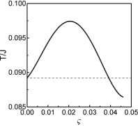
Figure 1: The evolution of the superconducting transition temperature with the strength of the electronic nematicity at the optimal doping $\delta=0.15$ for $t/J=3$ and $t^{\prime}/t=1/3$.

The enhancement of superconductivity by the electronic nematicity in cuprate superconductors implies that the energy in the SC-state with coexisting electronic nematicity is lower than the corresponding energy in the SC-state with the absence of the electronic nematicity, i.e., the SC-state with coexisting electronic nematicity is more stable than the SC-state with the absence of the electronic nematicity. In Appendix A.3, the evolution of the charge carrier pair gap parameter (then the electron pair gap parameter in Appendix A.6) with the strength of the electronic nematicity has been evaluated self-consistently, and the result of the maximal charge-carrier pair gap parameter $\bar{\Delta}^{\rm(h)}_{\varsigma{\rm max}}$ as a function of the strength of the electronic nematicity is plotted in Fig. 9, where with the increase of the strength of the electronic nematicity, $\bar{\Delta}^{\rm(h)}_{\varsigma{\rm max}}$ increases in the weak strength region, and achieves its maximum at around the same optimal strength of the electronic nematicity $\varsigma\approx 0.022$ as the nematic-order strength dependence of $T_{\rm c}$ shown in Fig. 1. However, with the further increase of the strength, $\bar{\Delta}^{\rm(h)}_{\varsigma{\rm max}}$ turns into a decrease in the strong strength region. Moreover, we Cao22 ; Zhao12 have also evaluated the ground-state energies both in the SC-state and normal-state with coexisting electronic nematicity, and found that the condensation energy $\Delta E^{(\varsigma)}_{\rm g}$ (then the energy difference between the normal-state energy and SC-state energy) is proportional to the charge-carrier pair gap parameter, i.e., $\Delta E^{(\varsigma)}_{\rm g}=E^{\rm(n)}_{\varsigma{\rm g}}-E^{\rm(s)}_{\varsigma{\rm g}}\propto\bar{\Delta}^{\rm(h)}_{\varsigma{\rm max}}$, which therefore shows that (i) the energy in the SC-state with coexisting electronic nematicity is lower than the SC-state energy with the absence of the electronic nematicity, indicating that the electronic nematicity together with the associated fluctuation phenomena in cuprate superconductors are a natural consequence of the strong electron correlation effect; (ii) the lowest energy in the SC-state with coexisting electronic nematicity occurs at around the same optimal strength of the electronic nematicity $\varsigma\approx 0.022$. This nematic-order strength dependence of the condensation energy and the related nematic-order strength dependence of the pair gap parameter thus explain why superconductivity is enhanced by the electronic nematicity, and $T_{\rm c}$ exhibits a dome-like shape nematic-order strength dependence. Furthermore, $T_{\rm c}$ as a function of the strength of the electronic nematicity at the doping $\delta=0.06$ has been obtained very recently in Ref. Cao21, . Incorporating the present result in Fig. 1 with that obtained in Ref. Cao21, , it is thus shown that although $T_{\rm c}$ for a given strength of the electronic nematicity at the doping $\delta=0.06$ is much lower than the corresponding $T_{\rm c}$ at the optimal doping $\delta=0.15$ shown in Fig. 1, the global dome-like shape of the nematic-order strength dependence of the enhancement of $T_{\rm c}$ at the doping $\delta=0.06$ together with the magnitude of the optimal strength obtained in Ref. Cao21, is the same with that at the optimal doping $\delta=0.15$ shown in Fig. 1, which therefore show that the enhancement of superconductivity by the electronic nematicity occurs at an any given doping concentration of the SC dome.

IV Electronic structure in superconducting-state with coexisting electronic nematicity

The electronic nematicity emerged as a key feature of cuprate superconductors has high impacts on various properties Vojta09 ; Fradkin10 ; Fernandes19 ; Lawler10 ; Fujita14 ; Zheng17 ; Fujita19 ; Nakata18 ; Hinkov08 ; Sato17 ; Daou10 ; Taillefer15 ; Wang21 ; Ando02 ; Wu17 ; Loret19 . In this section, we analyze the electronic structure of cuprate superconductors in the SC-state with coexisting electronic nematicity to shed light on the exotic features of the quasiparticle excitations. This nematic order coexist with spontaneous translation symmetry-breaking such as charge order leading to that the multiple modulations for the SC-state electronic structure occur simultaneously.

IV.1 Rotation symmetry-breaking of electron Fermi surface

Angle-resolved photoemission spectroscopy (ARPES) experiments Damascelli03 ; Campuzano04 ; Fink07 ; Zhou18 measure the single-particle excitation spectrum, while the underlying EFS contour in momentum space is directly obtained by the trace of the peak positions in the single-particle excitation spectrum. In the absence of any sort of symmetry-breaking, the shape of EFS of cuprate superconductors reflects the underlying symmetry of the square-lattice CuO₂ plane. In particular, the shape of EFS has deep consequences for the low-energy properties Timusk99 ; Hufner08 ; Vishik18 ; Comin16 ; Vojta09 ; Fradkin10 ; Fernandes19 , and has been also central to addressing multiple electronic orders Vojta09 ; Fradkin10 ; Fernandes19 ; Lawler10 ; Fujita14 ; Zheng17 ; Fujita19 ; Nakata18 ; Hinkov08 ; Sato17 ; Daou10 ; Taillefer15 ; Wang21 ; Ando02 ; Wu17 ; Loret19 . This is why the determination of the shape of EFS in cuprate superconductors is believed to be key issue for the understanding of the physical origin of different electronic ordered (then density-wave) states and of their intimate interplay with superconductivity.

In the absence of the rotation symmetry-breaking, we Gao18 ; Feng15a have shown within the framework of the kinetic-energy-driven superconductivity that although the EFS contour exhibits a $C_{4}$ rotation symmetry on the square lattice, the momentum dependence of the quasiparticle scattering due to the electron interaction by the exchange of a strongly dispersive spin excitation breaks up the EFS contour into the disconnected Fermi arcs with the most spectral weight that accommodates at around the tips of the Fermi arcs to form the Fermi-arc-tip liquid. As a natural consequence of the $C_{4}$ rotation symmetry on the square lattice, the two tips of the Fermi arc in each quarter of BZ are symmetrical about the nodal (diagonal) direction. Moreover, these tips of the Fermi arcs connected by the scattering wave vectors ${\bf q}_{i}$ construct an octet scattering model, where for any quasiparticle scattering process, the scattering wave vector and its symmetry-equivalent partner occur with equal amplitude. In this case, a bewildering variety of electronically ordered states with the translation symmetry-breaking described by the quasiparticle scattering processes with the corresponding scattering wave vectors ${\bf q}_{i}$ then are driven by this EFS instability Vishik18 ; Comin16 ; Vojta09 ; Wu11 ; Tacon12 ; Comin14 ; Neto14 ; Croft14 ; Hucker14 ; Campi15 ; Comin15 ; Peng16 . Although these electronically ordered states do not break the $C_{4}$ rotation symmetry on the square lattice, they break the discrete translation symmetry Vishik18 ; Comin16 ; Vojta09 ; Wu11 ; Tacon12 ; Comin14 ; Neto14 ; Croft14 ; Hucker14 ; Campi15 ; Comin15 ; Peng16 .

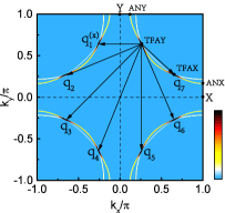
Figure 2: (Color online) The electron Fermi surface map at $\delta=0.15$ with $T=0.002J$ in the optimal strength of the electronic nematicity $\varsigma=0.022$ for $t/J=3$ and $t^{\prime}/t=1/3$, where ANX (ANY) and TFAX (TFAY) denote the antinode and tip of the Fermi arc near the X (Y) point of the Brillouin zone, respectively, and ${\bf q}_{1}$, ${\bf q}_{2}$, ${\bf q}_{3}$, ${\bf q}_{4}$, ${\bf q}_{5}$, ${\bf q}_{6}$, and ${\bf q}_{7}$ indicate different scattering wave vectors. However, the scattering wave vectors ${\bf q}_{1}$, ${\bf q}_{4}$, and ${\bf q}_{5}$ and the respective symmetry-corresponding partners occur with unequal amplitudes.

However, the original $C_{4}$ rotation symmetry in EFS is broken in the presence of the electronic nematicity. To understand this EFS anisotropy more clearly, we plot the map of the single-particle excitation spectral intensity $I({\bf k},0)$ in Eq. (8) at doping $\delta=0.15$ with temperature $T=0.002J$ in the optimal strength of the electronic nematicity $\varsigma=0.022$ in Fig. 2. Apparently, the electronic nematicity corresponds down to the $C_{2}$ rotation symmetry, where the most exotic features can be summarized as: (i) the original EFS with the $C_{4}$ rotation symmetry on the square lattice in the absence of the electronic nematicity is broken up into that with a residual $C_{2}$ rotation symmetry, which leads to the EFS distortion. As a natural consequence, the electronic structure at around the antinode near the X point (ANX) of BZ is inequivalent to that at around the antinode near the Y point (ANY). In particular, with the increase of the strength of the electronic nematicity, the antinode near the X point of BZ shifts away from the $[\pi,0]$ point, while the antinode near the Y point moves towards to the $[0,\pi]$ point, in qualitative agreement with the ARPES experimental results Nakata18 . Moreover, as in the case of the absence of the electronic nematicity Gao18 , a bifurcation for the original single-contour EFS occurs due to the renormalization of the electrons in the presence of the strong electron interaction mediated by a strongly dispersive spin excitation except for at around the tips of the Fermi arcs, where this bifurcation disappears. However, the spectral weight on the extra sheet is suppressed, leading to that this extra sheet become unobservable in experiments; (ii) although the special feature of the most spectral weight that accommodates at around the tips of the Fermi arcs remains, the symmetrical relation of two tips of the Fermi arc in each quarter of BZ about the nodal (diagonal) direction vanishes; (iii) concomitantly, the original $C_{4}$ rotation symmetry for the octet scattering model in the absence of the electronic nematicity is broken into the $C_{2}$ rotation symmetry, where for the partial quasiparticle scattering processes with the corresponding scattering wave vectors ${\bf q}_{1}$, ${\bf q}_{4}$, and ${\bf q}_{5}$, the amplitudes of the scattering wave vectors are respectively inequivalent to their symmetry-corresponding partners. This EFS instability in the presence of the electronic nematicity then drives multiple ordered states, where the electronic ordered states described by the quasiparticle scattering processes with the corresponding scattering wave vectors ${\bf q}_{1}$, ${\bf q}_{4}$, and ${\bf q}_{5}$ break both the rotation and translation symmetries, while these ordered states described by the quasiparticle scattering processes with the corresponding scattering wave vectors ${\bf q}_{2}$, ${\bf q}_{3}$, ${\bf q}_{6}$, and ${\bf q}_{7}$ only break the translation symmetry. In particular, the charge-order wave vector $Q^{(x)}_{\rm co}={\bf q}^{(x)}_{1}$ is on amplitude an inequality with its symmetry-corresponding partner $Q^{(y)}_{\rm co}={\bf q}^{(y)}_{1}$, i.e., $Q^{(x)}_{\rm co}\neq Q^{(y)}_{\rm co}$, leading to the emergence of the most significant stripe type charge order with broken both rotation and translation symmetries Comin15a ; Zhang18 , i.e., this stripe type charge order has a nematic character. Furthermore, as in the case without the rotation symmetry-breaking Gao18 , the positions of the tips of the Fermi arcs are doping dependent, which therefore leads to the evolution of the amplitudes of the scattering wave vectors ${\bf q}_{i}$ with doping. More specifically, the magnitude of the charge-order wave vector $Q_{\rm co}$ smoothly decreases with the increase of doping Gao18 , in qualitative agreement with the experimental data Vishik18 ; Comin16 ; Vojta09 ; Wu11 ; Tacon12 ; Comin14 ; Neto14 ; Croft14 ; Hucker14 ; Campi15 ; Comin15 ; Peng16 . This octet scattering model with the $C_{2}$ rotation symmetry shown in Fig. 2 is a fundamental quasiparticle scattering model Wang03 ; Gao19 in the explanation of the rotation symmetry-breaking of the QSI experimental data Lawler10 ; Fujita14 ; Zheng17 ; Fujita19 , and also can give a consistent description of the regions of the highest joint density of states observed from the ARPES autocorrelation experiments Wang03 ; Gao19 ; Chatterjee06 ; He14 . We will return to this discussion towards Sec. V of this paper.

Within the framework of the kinetic-energy-driven superconductivity Feng15 ; Feng0306 ; Feng12 ; Feng15a , the SC quasiparticles are the phase-coherent linear superpositions of electrons and holes as in the conventional superconductors, while the SC condensate is made up of electron pairs, which are bound-states of two electrons with opposite momenta and spins. On the other hand, the electronically ordering quasiparticles are superpositions of electrons (or holes), and then the electronically ordered state is likewise a pair condensate, but of electrons and holes, whose net momentum determines the wave-length of electronic ordering Gao18 ; Kohn70 ; Hinton16 . In the presence of the electronic nematicity, the pairing of electrons and holes at ${\bf k}$ and ${\bf k}+{\bf q}_{i}$ separated by the electronic order wave vector ${\bf q}_{i}$ drives the symmetry-breaking ordered state formation, whereas the electron pairing at ${\bf k}$ and ${-\bf k}$ states induces superconductivity. This is why the SC-state of cuprate superconductors coexists with a bewildering variety of the electronically ordered states with the symmetry-breaking, leading to that the multiple modulations for the SC-state occur simultaneously.

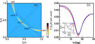
Figure 3: (Color online) (a) The intensity map of the quasiparticle scattering rate and (b) the angular dependence of the quasiparticle scattering rate along the electron Fermi surface from the antinode near the X point of the Brillouin zone to the node (red line) and from the antinode near the Y point to the node (blue line) at $\delta=0.15$ with $T=0.002J$ in the optimal strength of the electronic nematicity $\varsigma=0.022$ for $t/J=3$ and $t^{\prime}/t=1/3$, where ANX (ANY) and TFAX (TFAY) in (a) denote the positions of the antinode and tip of the Fermi arc near the X (Y) point, respectively, and ND denotes the position of the node, while the red (blue) arrow in (b) indicates the corresponding minimum of the quasiparticle scattering rate (then the corresponding position of the tip of the Fermi arc).

The above obtained $C_{4}$ rotation symmetry-breaking of EFS is caused by the electronic nematicity, while the EFS reconstruction to form the disconnected Fermi arcs is still attributed to the momentum dependence of the quasiparticle scattering rate Feng16 ; Gao18 $\Gamma_{\varsigma}({\bf k},0)={\rm Im}\Sigma^{(\varsigma)}_{\rm tot}({\bf k},0)$. This follows a basic fact that in despite of the presence of the electronic nematicity, the EFS contour in momentum space is determined directly by the poles of the full electron diagonal propagator (3a) at zero energy,

$$\varepsilon^{(\varsigma)}_{{\bf k}_{\rm F}}-{\rm Re}\Sigma^{(\varsigma)}_{\rm tot}({\bf k}_{\rm F},0)=0,$$ (9)

and then the spectral weight on the EFS contour is dominated mainly by the inverse of the quasiparticle scattering rate $1/\Gamma_{\varsigma}({\bf k}_{\rm F},0)$. However, the electronic nematicity generates a breaking of the symmetrical relation of $\Gamma_{\varsigma}({\bf k}_{\rm F},0)$ about the nodal (diagonal) direction. To pinpoint this origin of EFS with broken rotation symmetry, we plot (a) the intensity map of $\Gamma_{\varsigma}({\bf k}_{\rm F},0)$ and (b) the angular dependence of $\Gamma_{\varsigma}({\bf k}_{\rm F},0)$ at $\delta=0.15$ with $T=0.002J$ in the optimal strength of the electronic nematicity $\varsigma=0.022$ in Fig. 3, where the three exotic features emerge as: (i) The quasiparticle scattering is stronger at around the antinodal region than at around the nodal region. In this case, the spectral weight on the EFS contour ${\bf k}_{\rm F}$ at around the antinodal region is substantially suppressed, while the spectral weight at around the nodal region is reduced modestly, which leads to form the disconnected Fermi arcs around the nodal region; (ii) The weakest quasiparticle scattering does not occur at around the node, but occurs exactly at the tips of the Fermi arcs, which further reduces the most part of the spectral weight on the Fermi arcs to the tips of the Fermi arcs. This angular dependences of $\Gamma_{\varsigma}({\bf k}_{\rm F},0)$ is in qualitative agreement with the experimental data Vishik09 , where the weakest quasiparticle scattering appeared at around the tips of the Fermi arcs has been observed. These tips of the Fermi arcs connected by the scattering wave vectors ${\bf q}_{i}$ therefore construct an octet scattering model; (iii) However, the positions of the strongest scattering at the antinode and the weakest scattering at the tip of the Fermi arc near X point of BZ are clearly different from the corresponding positions of the strongest scattering at the antinode and the weakest scattering at the tip of the Fermi arc near Y point, and then the symmetrical relation of $\Gamma_{\varsigma}({\bf k}_{\rm F},0)$ about the nodal (diagonal) direction disappears. This anisotropy of $\Gamma_{\varsigma}({\bf k}_{\rm F},0)$ therefore induces EFS with broken $C_{4}$ rotation symmetry shown in Fig. 2. Moreover, the positions of the weakest quasiparticle scattering is doping dependent, which therefore leads to the positions of the tips of the Fermi arcs (then the scattering wave vectors ${\bf q}_{i}$ in the octet scattering model) are the evolution with doping.

IV.2 Line-shape anisotropy of energy distribution curve

We now turn to our attention to the anisotropy of the electronic structure of cuprate superconductors in the SC-state with coexisting electronic nematicity. The most intuitive approach is to analyze section corresponding to a fixed momentum ${\bf k}$, i.e., the energy distribution curve, where the characteristic feature is so-called peak-dip-hump (PDH) structure Dessau91 ; Randeria95 ; Norman97 ; Campuzano99 ; DLFeng02 ; Wei08 ; Hashimoto15 ; DMou17 . This remarkable PDH structure consists of a sharp quasiparticle excitation peak at the lowest binding-energy, a broad hump at the higher binding-energy, and a spectral dip between them. Theoretical, there is a general consensus that the emergence of the dip is a natural consequence of very strong scattering of the electrons mediated by bosonic excitations, although what type bosonic excitation that is the appropriate bosonic excitation for the role of the electron pairing glue is still under debate. In particular, both the experimental and theoretical studies indicate that the sharp peak in the quasiparticle scattering rate is directly responsible for the outstanding PDH structure in the energy distribution curve DMou17 ; Gao18a ; Liu20a .

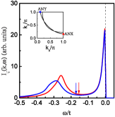
Figure 4: (Color online) The energy distribution curves at the antinode near the X point of the Brillouin zone (red line) and at the antinode near the Y point (blue line) in $\delta=0.15$ with $T=0.002J$ and the optimal strength of the electronic nematicity $\varsigma=0.022$ for $t/J=3$ and $t^{\prime}/t=1/3$, where the arrows indicate the positions of the dips, while ANX and ANY in the inset denote the antinodes near the X and Y points, respectively.

In the absence of the electronic nematicity, the line-shape of the energy distribution curve exhibits the $C_{4}$ rotation symmetry on the square lattice, reflecting a basic fact that the electronic structure is equivalent between the $k_{x}$ and $k_{y}$ directions in momentum space Dessau91 ; Randeria95 ; Norman97 ; Campuzano99 ; DLFeng02 ; Wei08 ; Hashimoto15 ; DMou17 . However, in corresponding to the $C_{4}$ rotation symmetry-breaking of EFS shown in Fig. 2, the electronic nematicity induces the line-shape anisotropy of the energy distribution curve. To see this point more clearly, we plot the energy distribution curves at the antinode near the X point of BZ (red line) and at the antinode near the Y point (blue line) for $\delta=0.15$ with $T=0.002J$ in the optimal strength of the electronic nematicity $\varsigma=0.022$ in Fig. 4, where although the global feature of the PDH structure in the energy distribution curve is in a striking analogy to that in the corresponding case without the rotation symmetry-breaking, the line-shape of the energy distribution curve at the antinode near the X point of BZ is not identical with that at the antinode near the Y point, leading to the line-shape anisotropy of the energy distribution curve. In particular, the spectral intensities are higher at the antinode near X point than at the antinode near Y point, in agreement with the ARPES experimental results Nakata18 . Moreover, the hump and dip energies in the PDH structure at the antinode near the X point is lower than the corresponding hump and dip energies at the antinode near the Y point, respectively, which also conform to the result of EFS with the $C_{2}$ rotation symmetry shown in Fig. 2. However, it should be noted that although the electronic structure becomes inequivalent between the $k_{x}$ and $k_{y}$ directions, the electronic structure along the nodal direction is unaffected, also in agreement with the ARPES experimental results Nakata18 .

This inequivalence of the electronic structure between the $k_{x}$ and $k_{y}$ directions associated with the electronic nematicity can be also interpreted in terms of the quasiparticle scattering rate anisotropy. The origin of the emergence of the PDH structure in the energy distribution curve is intimately related to the corresponding peak-structure in the quasiparticle scattering rate generated from the electron interaction by the exchange of a strongly dispersive spin excitation DMou17 ; Gao18a ; Liu20a . From the single-particle excitation spectrum in Eq. (8), the position of the peak in the energy distribution curve is determined by the renormalized quasiparticle excitation energy in terms of the self-consistent equation,

$$\omega-\varepsilon^{(\varsigma)}_{\bf k}-{\rm Re}\Sigma^{(\varsigma)}_{\rm tot}({\bf k},\omega)=0,$$ (10)

and then the intensity of this peak is dominated by the inverse of the quasiparticle scattering rate $\Gamma_{\varsigma}({\bf k},\omega)$ [then the imaginary part of the total self-energy ${\rm Im}\Sigma^{(\varsigma)}_{\rm tot}({\bf k},\omega)$]. In other words, the spectral line-shape in the energy distribution curve is determined by both the real and imaginary parts of the total self-energy. However, in the presence of the electronic nematicity, the peak energy of $\Gamma_{\varsigma}({\bf k},\omega)$ is lower at the antinode near the X point than at the antinode near the Y point, leading to the inequivalence of the line-shape between the antinodes near X and Y points. To test this idea directly, we plot the quasiparticle scattering rate $\Gamma_{\varsigma}({\bf k},\omega)$ as a function of energy at the antinode near the X point (red line) and at the antinode near the Y point (blue line) for $\delta=0.15$ with $T=0.002J$ in the optimal strength of the electronic nematicity $\varsigma=0.022$ in Fig. 5, where $\Gamma_{\varsigma}({\bf k},\omega)$ exhibits a sharp peak-structure at both the antinodes near the X and Y points, with the position of the peak in $\Gamma_{\varsigma}({\bf k},\omega)$ at the antinode near the X (Y) point corresponds exactly to the position of the dip in the PDH structure at the antinode near the X (Y) point shown in Fig. 4, indicating that the peak-structure in $\Gamma_{\varsigma}({\bf k},\omega)$ is responsible directly for the PDH structure in the energy distribution curve DMou17 ; Gao18a ; Liu20a . However, the peak energy in $\Gamma_{\varsigma}({\bf k},\omega)$ at the antinode near the X point is different from that at the antinode near the Y point, which leads to the inequivalence of the line-shape in the energy distribution curve between the antinodes near X and Y points. Moreover, the intensity of the peak in $\Gamma_{\varsigma}({\bf k},\omega)$ at the antinode near the Y point is higher than that at the antinode near the X point, this is why the spectral intensities shown in Fig. 4 are higher at the antinode near X point than at the antinode near Y point.

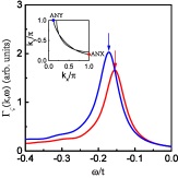
Figure 5: (Color online) The quasiparticle scattering rate as a function of energy at the antinode near the X point of the Brillouin zone (red line) and at the antinode near the Y point (blue line) in $\delta=0.15$ with $T=0.002J$ and the optimal strength of the electronic nematicity $\varsigma=0.022$ for $t/J=3$ and $t^{\prime}/t=1/3$, where the arrows indicate the positions of the peaks, while ANX and ANY in the insets denote the antinodes near the X and Y points, respectively.

V Quantitative characteristics of rotation symmetry-breaking of quasiparticle scattering interference

The exploration of QSI in cuprate superconductors can be used to elucidate the nature of the quasiparticle excitation and of its interplay with symmetry-breaking orders and superconductivity. This follows an experimental fact that the quasiparticles scattering from impurities interfere with one another, producing a notable QSI pattern in the inhomogeneous part for the Fourier transform (FT) of the scanning tunneling spectroscopy (STS) measured real-space image of the local density of states (LDOS) Yin21 ; Pan01 ; Hoffman02 ; Kohsaka07 ; Kohsaka08 ; Hamidian16 . From these observed QSI patterns as a function of energy, one can obtain the energy variation of the momentum ${\bf q}$, which is an autocorrelation between the electronic bands $E_{\bf k}$ and $E_{{\bf k}+{\bf q}}$. For the same band $E_{\bf k}$, the intensity distribution of the QSI pattern can be different, depending on the quasiparticle scattering geometry. However, this quasiparticle scattering geometry is closely associated with the shape of EFS and the related electron distribution, which are directly related to the single-particle excitation spectrum. In other words, the QSI intensity is proportional to the intensities of the single-particle excitation spectra at the momenta ${\bf k}$ and ${\bf k}+{\bf q}$, while the intensity peaks in the QSI pattern then are corresponding to the highest joint density of states. This is why the dispersion of the peaks in the QSI pattern as a function of energy is analyzed in terms of the octet scattering model shown in Fig. 2 and yields the crucial information about the shape of EFS and the related nature of the quasiparticle excitation. Moreover, by the measurement of the characteristic feature of the Bragg peaks in FT of a real-space image of LDOS, one is considering the phenomena that occur with the periodicity of the underlying square lattice and which qualify any rotation symmetry-breaking. On the other hand, the ARPES autocorrelation Chatterjee06 ; He14 ,

$${\bar{C}}_{\varsigma}({\bf q},\omega)={1\over N}\sum_{\bf k}I_{\varsigma}({\bf k}+{\bf q},\omega)I_{\varsigma}({\bf k},\omega),$$ (11)

measures the autocorrelation of the single-particle excitation spectra in Eq. (8) at two different momenta ${\bf k}$ and ${\bf k}+{\bf q}$, where the summation of momentum ${\bf k}$ is extended up to the second BZ for the discussion of QSI together with the Bragg scattering Chatterjee06 , and $N$ is the number of lattice sites. This ARPES autocorrelation in Eq. (11) therefore detects the effectively momentum-resolved joint density of states in the electronic state, and can give us the important insights into the nature of the quasiparticle excitation. In particular, the experimental observations Chatterjee06 ; He14 have demonstrated that the ARPES autocorrelation exhibits discrete spots in momentum-space, which are directly related with the quasiparticle scattering wave vectors ${\bf q}_{i}$ connecting the tips of the Fermi arcs in the octet scattering model shown in Fig. 2, and are also well consistent with the QSI peaks observed from the FT-STS experiments Yin21 ; Pan01 ; Hoffman02 ; Kohsaka07 ; Kohsaka08 ; Hamidian16 . Moreover, we Gao19 have also shown within the framework of the kinetic-energy-driven superconductivity that there is an intimate connection of the ARPES autocorrelation with QSI in cuprate superconductors, where the inhomogeneous part for FT LDOS in the presence of a single point-like impurity scattering potential has been evaluated based on the octet scattering model, and then the obtained momentum-space structure of the QSI patterns in the presence of the strong scattering potential is well consistent with the momentum-space structure of the ARPES autocorrelation patterns. In other words, the octet scattering model with the quasiparticle scattering wave vectors ${\bf q}_{i}$ connecting the corresponding tips of the Fermi arcs that can give a consistent description of the regions of the highest joint density of states in the ARPES autocorrelation can be also used to explain the QSI data observed from the FT-STS experiments. This is also why the main features of QSI Yin21 ; Pan01 ; Hoffman02 ; Kohsaka07 ; Kohsaka08 ; Hamidian16 can be also obtained in terms of the ARPES autocorrelation Chatterjee06 ; He14 . However, the original electronic structure with the $C_{4}$ rotation symmetry is thus broken in the presence of the electronic nematicity, while such an aspect should be reflected in the corresponding QSI. In this subsection, we discuss the characteristic feature of the rotation symmetry-breaking of QSI in terms of the ARPES autocorrelation, and then make a comparison with the results of the rotation symmetry-breaking QSI measured from the FT-STS experiments Lawler10 ; Fujita14 ; Zheng17 ; Fujita19 .

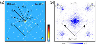
Figure 6: (Color online) (a) The intensity map of the ARPES autocorrelation in a $[q_{x},q_{y}]$ plane at the binding-energy $\omega=94$ meV and $\delta=0.06$ with $T=0.002J$ and the optimal strength of the electronic nematicity $\varsigma=0.022$ for $t/J=3$ and $t^{\prime}/t=1/3$. ${\bf q}_{1}$, ${\bf q}_{2}$, ${\bf q}_{3}$, ${\bf q}_{4}$, ${\bf q}_{5}$, ${\bf q}_{6}$, and ${\bf q}_{7}$ in (a) indicate different scattering wave vectors, however, the scattering wave vectors ${\bf q}_{1}$, ${\bf q}_{4}$, and ${\bf q}_{5}$ and the respective symmetry-corresponding partners occur with unequal amplitudes. The locations of the Bragg peaks ${\bf Q}^{\rm(B)}_{x}$ and ${\bf Q}^{\rm(B)}_{y}$ in (a) are indicated by circles. (b) The corresponding experimental result of the quasiparticle scattering interference pattern for Bi₂Sr₂CaCu₂O_8+δ at doping $\delta=0.06$ in the binding-energy $\omega=94$ meV taken from Ref. Fujita19, .

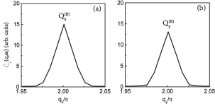
Figure 7: The intensity of the peak as a function of momentum (a) at around the Bragg wave vector ${\bf Q}^{\rm(B)}_{x}$ along the $q_{x}$ direction and (b) at around the Bragg wave vector ${\bf Q}^{\rm(B)}_{y}$ along the $q_{y}$ direction in the binding-energy $\omega=94$ meV and $\delta=0.06$ with $T=0.002J$ and the optimal strength of the electronic nematicity $\varsigma=0.022$ for $t/J=3$ and $t^{\prime}/t=1/3$.

Now we are ready to discuss the characteristic feature of QSI together with the Bragg scattering in the SC-state with coexisting nematic order. We have made a series of calculations for the ARPES autocorrelation ${\bar{C}}_{\varsigma}({\bf q},\omega)$, and the results show that the breaking of the $C_{4}$ rotation symmetry also occurs in the ARPES autocorrelation pattern (then the QSI pattern). To see this exotic feature more clearly, we plot the intensity map of ${\bar{C}}_{\varsigma}({\bf q},\omega)$ in a $[q_{x},q_{y}]$ plane for the binding-energy $\omega=94$ meV at $\delta=0.06$ with $T=0.002J$ and the optimal strength of the electronic nematicity $\varsigma=0.022$ in Fig. 6a, where the positions of the Bragg peaks ${\bf Q}^{\rm(B)}_{x}$ and ${\bf Q}^{\rm(B)}_{y}$ are labelled by circles, while ${\bf q}_{1}$, ${\bf q}_{2}$, ${\bf q}_{3}$, ${\bf q}_{4}$, ${\bf q}_{5}$, ${\bf q}_{6}$, and ${\bf q}_{7}$ indicate different scattering wave vectors, however, the scattering wave vectors ${\bf q}_{1}$, ${\bf q}_{4}$, and ${\bf q}_{5}$ and the respective symmetry-corresponding partners occur with unequal amplitudes as in the case shown in Fig. 2. For a comparison, the corresponding experimental result Fujita19 of the QSI pattern observed from Bi₂Sr₂CaCu₂O_8+δ at doping $\delta=0.06$ for the bind-energy $\omega=94$ meV is also shown in Fig. 6b. Obviously, the experimental result Fujita19 of the momentum-space structure of the QSI pattern is qualitatively reproduced, where two distinct classes of the broken-symmetry states in Fig. 6a have emerged as: (i) The Bragg peaks at the wave vectors ${\bf Q}^{\rm(B)}_{x}=[\pm 2\pi,0]$ along the $\hat{x}$ axis and ${\bf Q}^{\rm(B)}_{y}=[0,\pm 2\pi]$ along the $\hat{y}$ axis, which are the signature of the nematic-order state with the broken $C_{4}$ rotation symmetry, since the intensity of the peak at the Bragg wave vector ${\bf Q}^{\rm(B)}_{x}$ is different from that at the Bragg wave vector ${\bf Q}^{\rm(B)}_{y}$. To see this difference more clearly, we plot ${\bar{C}}_{\varsigma}({\bf q},\omega)$ as a function of momentum at around (a) the Bragg wave vector ${\bf Q}^{\rm(B)}_{x}$ along the $q_{x}$ direction and (b) at around the Bragg wave vector ${\bf Q}^{\rm(B)}_{y}$ along the $q_{y}$ direction in the binding-energy $\omega=94$ meV for $\delta=0.06$ with $T=0.002J$ and the optimal strength of the electronic nematicity $\varsigma=0.022$ in Fig. 7, where when the momentum is turned away from the Bragg wave vector ${\bf Q}^{\rm(B)}_{x}$ $({\bf Q}^{\rm(B)}_{y})$, the distinct peak at the Bragg wave vector ${\bf Q}^{\rm(B)}_{x}$ $({\bf Q}^{\rm(B)}_{y})$ is suppressed rapidly, and then eventually disappears. More importantly, the intensity of the peak at the Bragg wave vector ${\bf Q}^{\rm(B)}_{x}$ is higher than that at the Bragg wave vector ${\bf Q}^{\rm(B)}_{y}$, in qualitative agreement with the experimental observation from the STS measurements Lawler10 ; Fujita14 ; Zheng17 ; Fujita19 . Furthermore, ${\bar{C}}_{\varsigma}({\bf q},\omega)$ as a function of momentum at around the Bragg wave vector ${\bf Q}^{\rm(B)}_{x}$ along the $q_{y}$ direction and at around the Bragg wave vector ${\bf Q}^{\rm(B)}_{y}$ along the $q_{x}$ direction have been also calculated, and the similar results as shown in Fig. 7 are obtained. This difference of the intensities of the Bragg peak between the Bragg wave vectors ${\bf Q}^{\rm(B)}_{x}$ and ${\bf Q}^{\rm(B)}_{y}$ shows the inequivalence on the average of the electronic structure at the two Bragg scattering sites ${\bf Q}^{\rm(B)}_{x}$ and ${\bf Q}^{\rm(B)}_{y}$, and therefore verifies the $C_{4}$ rotation symmetry-breaking in the presence of the nematic order; (ii) The peaks at the scattering wave vectors ${\bf q}_{1}$, ${\bf q}_{4}$, and ${\bf q}_{5}$, which are the signatures of the multiple ordered states with broken both rotation and translation symmetries, while the peaks at the scattering wave vectors ${\bf q}_{2}$, ${\bf q}_{3}$, ${\bf q}_{6}$, and ${\bf q}_{7}$, which are the signatures of the multiple ordered states with broken translation symmetry. These results are also expected from the octet scattering model shown in Fig. 2 with broken $C_{4}$ rotation symmetry.

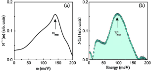
Figure 8: (Color online) (a) The energy evolution of the order parameter of the nematic-order state at $\delta=0.06$ with $T=0.002J$ in the optimal strength of the electronic nematicity $\varsigma=0.022$ for $t/J=3$, $t^{\prime}/t=1/3$, and $J=100$ meV, where the arrow indicates the positions of the peak. (b) The corresponding experimental result observed on Bi₂Sr₂CaCu₂O_8+δ at doping $\delta=0.06$ taken from Ref. Fujita19, .

Following the common practice, the order parameter of the electronic nematicity can be properly represented as a traceless symmetric tensor Fradkin10 . In the present case in which the nematic order is associated with the breaking of the $C_{4}$ rotation symmetry in the underlying square-lattice CuO₂ plane, the order parameter of the electronic nematicity is defined by principle as,

$$N^{({\bar{C}}_{\varsigma})}_{0}(\omega)={{\bar{C}}_{\varsigma}({\bf Q}^{\rm(B)}_{x},\omega)-{\bar{C}}_{\varsigma}({\bf Q}^{\rm(B)}_{y},\omega)\over{\bar{C}}_{\varsigma}({\bf Q}^{\rm(B)}_{x},\omega)+{\bar{C}}_{\varsigma}({\bf Q}^{\rm(B)}_{y},\omega)}.$$

However, as we have mentioned in Sec. II, the calculation for the normal and anomalous self-energies in Eq. (6) is performed numerically on a $120\times 120$ lattice in momentum space, with the infinitesimal $i0_{+}\rightarrow i\Gamma$ replaced by a small damping $\Gamma=0.05J$, which leads to that the peak weight of the ARPES autocorrelation ${\bar{C}}_{\varsigma}({\bf q},\omega)$ in Eq. (11) at the Bragg wave vector ${\bf Q}^{\rm(B)}_{x}$ $[{\bf Q}^{\rm(B)}_{y}]$ spreads on the extremely small area $\{{\bf Q}^{\rm(B)}_{x}\}$ $[\{{\bf Q}^{\rm(B)}_{y}\}]$ around the ${\bf Q}^{\rm(B)}_{x}$ $[{\bf Q}^{\rm(B)}_{y}]$ point as shown in Fig. 7a [Fig. 7b]. In particular, the summation of these spread weights around this extremely small area $\{{\bf Q}^{\rm(B)}_{x}\}$ $[\{{\bf Q}^{\rm(B)}_{y}\}]$ is less affected by the calculation for a finite lattice. In this case, a more appropriate order parameter of the electronic nematicity can be defined as,

$$N^{({\bar{C}}_{\varsigma})}(\omega)={{\bar{C}}^{(x)}_{\varsigma}(\omega)-{\bar{C}}^{(y)}_{\varsigma}(\omega)\over{\bar{C}}^{(x)}_{\varsigma}(\omega)+{\bar{C}}^{(y)}_{\varsigma}(\omega)},$$ (12)

for the reduction of the size effect in the finite-lattice calculation, where ${\bar{C}}^{(x)}_{\varsigma}(\omega)=(1/N)\sum_{{\bf q}\in\{{\bf Q}^{\rm(B)}_{x}\}}{\bar{C}}_{\varsigma}({\bf q},\omega)$ and ${\bar{C}}^{(y)}_{\varsigma}(\omega)=(1/N)\sum_{{\bf q}\in\{{\bf Q}^{\rm(B)}_{y}\}}{\bar{C}}_{\varsigma}({\bf q},\omega)$, with the summation ${\bf q}\in\{{\bf Q}^{\rm(B)}_{x}\}$ $[{\bf q}\in\{{\bf Q}^{\rm(B)}_{y}\}]$ that is restricted to the extremely small area $\{{\bf Q}^{\rm(B)}_{x}\}$ $[\{{\bf Q}^{\rm(B)}_{y}\}]$ around ${\bf Q}^{\rm(B)}_{x}$ $[{\bf Q}^{\rm(B)}_{y}]$. This order parameter $N^{({\bar{C}}_{\varsigma})}(\omega)$ is identically zero in the state without the $C_{4}$ rotation symmetry-breaking, and non-zero in the nematic-order state with broken $C_{4}$ rotation symmetry. We have carried out a series of calculation for the order parameter $N^{({\bar{C}}_{\varsigma})}(\omega)$, and the result shows that order parameter $N^{({\bar{C}}_{\varsigma})}(\omega)|_{\omega=94{\rm meV}}\sim 0.1\neq 0$ in the binding-energy $\omega=94$ meV. This non-zero order parameter further confirms the breaking of the $C_{4}$ rotation symmetry-breaking in the ARPES autocorrelation (then QSI) shown in Fig. 6 in the presence of the electronic nematicity. Moreover, this order parameter $N^{({\bar{C}}_{\varsigma})}(\omega)$ is strongly energy dependent. To see this strong energy dependence of the order parameter more clearly, we plot $N^{({\bar{C}}_{\varsigma})}(\omega)$ as a function of binding-energy at $\delta=0.06$ with $T=0.002J$ in the optimal strength of the electronic nematicity $\varsigma=0.022$ in Fig. 8a. For a comparison, the corresponding experimental result Fujita19 of the energy dependence of the order parameter of the electronic nematicity observed from Bi₂Sr₂CaCu₂O_8+δ at doping $\delta=0.06$ is also shown in Fig. 8b. Obviously, the global feature of the obtained energy dependence of the order parameter exhibits qualitatively resemblance to the corresponding experimental data Fujita19 . This order parameter $N^{({\bar{C}}_{\varsigma})}(\omega)$ starts to grow continuously with the increase of binding-energy in the lower energy range, and achieves its maximum in the energy $\omega_{\rm max}\sim 1.4J$, then decrease rapidly with the increase of binding-energy in the higher energy range. In particular, this anticipated characteristic energy $\omega_{\rm max}\sim 1.4J=140$ meV is not too far from $E^{(N)}_{\rm max}\sim 94$ meV observed from the QSI patterns Fujita19 in Bi₂Sr₂CaCu₂O_8+δ at doping $\delta=0.06$. In this case, the electronic nematicity verified using the order parameter $N^{({\bar{C}}_{\varsigma})}(\omega)$ indeed derives primarily from the inequivalence of the electronic structure at the two Bragg scattering sites ${\bf Q}^{\rm(B)}_{x}$ and ${\bf Q}^{\rm(B)}_{y}$. However, it should be emphasized that the magnitude of the characteristic energy $\omega_{\rm max}$ is also dependent on the strength of the electronic nematicity. In particular, for the strength of the electronic nematicity $\varsigma=0.006$, the corresponding $\omega_{\rm max}\sim 0.936J=93.6$ meV, which is well consistent with the experimental result Fujita19 of $E^{(N)}_{\rm max}\sim 94$ meV.

Experimentally, by measuring tunneling conductance of Bi₂Sr₂CaCu₂O_8+δ over a large field of view, performing a FT, and analyzing data from distinct regions of momentum space Fujita19 , the pseudogap energy $\Delta^{*}$, the charge-order characteristic energy $\Delta^{\rm(co)}_{\rm max}$, and the electronic nematicity characteristic energy $\omega_{\rm max}$ have been identified, where measured on the samples whose doping spans the pseudogap regime, $\omega_{\rm max}$, $\Delta^{\rm(co)}_{\rm max}$, and $\Delta^{*}$ are, within the experimental error, identical Fujita19 . These experimental observations therefore strongly suggest that the nematic and charge orders are tied to the pseudogap. On the theoretical hand, we Cao21 have studied very recently the doping dependence of the electronic nematicity characteristic energy in cuprate superconductors, and the obtained result is fully consistent with the corresponding result Fujita19 observed on Bi₂Sr₂CaCu₂O_8+δ. In particular, the obtained doping dependence of the electronic nematicity characteristic energy is also in good agreement with the corresponding doping dependence of the pseudogap energy $\Delta^{*}$ over a wide range of doping Fujita19 . The pseudogap in the framework of the kinetic energy driven superconductivity originates from the electron self-energy Feng12 ; Feng15a , and then it can be identified as being a region of the electron self-energy effect in which the pseudogap suppresses the spectral weight of the quasiparticle excitation spectrum. The present study together with the study in Ref. Cao21, thus show that the pseudogap regime harbours diverse manifestations of the electronically ordered phases, and then a characteristic feature in the complicated phase diagram of cuprate superconductors is the coexistence and intertwinement of different ordered states and superconductivity. Moreover, the nematic-order state strength dependence of the characteristic energy $\omega_{\rm max}$ has been also discussed Cao21 , and the result shows that the nematic-order state strength dependence of the characteristic energy $\omega_{\rm max}$ coincides with the corresponding nematic-order state strength dependence of the enhancement of $T_{\rm c}$, suggesting a possible connection between the electronic nematicity characteristic energy and the enhancement of the superconductivity.

VI Summary and discussions

Within the framework of the kinetic-energy-driven superconductivity, we have investigated the intertwinement of the electronic nematicity with superconductivity in cuprate superconductors. The obtained phase diagram shows that the magnitude of the optimized $T_{\rm c}$ is found to increase gradually with the increase of the strength of the electronic nematicity in the weak strength region, and reaches its maximum in the optimal strength of the electronic nematicity, then monotonically decreases with the increase of the strength of the electronic nematicity in the strong strength region, in a striking similar to the dome-like shape doping dependence of $T_{\rm c}$. This dome-like shape nematic-order strength dependence of $T_{\rm c}$ therefore indicates that superconductivity in cuprate superconductors is enhanced by the electronic nematicity. Our results also show that the electronic nematicity has high impacts on the electronic structure, where (i) the original EFS contour with the $C_{4}$ rotation symmetry is broken up into that with a residual $C_{2}$ rotation symmetry, leading to the EFS anisotropy. However, this EFS contour with the $C_{2}$ rotation symmetry still shrinks down to form the disconnected Fermi arcs with the most spectral weight that accommodates at around the tips of the Fermi arcs; (ii) although the tips of the Fermi arcs connected by the scattering wave vectors ${\bf q}_{i}$ still construct an octet scattering model, for the partial quasiparticle scattering processes with the corresponding scattering wave vectors ${\bf q}_{1}$, ${\bf q}_{4}$, and ${\bf q}_{5}$, the amplitudes of the scattering wave vectors are respectively inequivalent to their symmetry-corresponding partners, leading to the rotation symmetry-breaking of the octet scattering model; (iii) the line-shape of the energy distribution curve is inequivalent between the antinodal region near the X point of BZ and the antinodal region near the Y point, leading to the electronic structure anisotropy. Moreover, these anisotropic features of the electronic structure obtained from the single-particle excitation spectrum are also confirmed via the results of QSI described in terms of the ARPES autocorrelation, where the breaking of the $C_{4}$ rotation symmetry is verified by the inequivalence on the average of the electronic structure at the two Bragg scattering sites. The theoretical results also indicate that the order parameter of the electronic nematicity achieves its maximum in the characteristic energy $\omega_{\rm max}$, however, when the energy is tuned away from this characteristic energy $\omega_{\rm max}$, the order parameter of the electronic nematicity decreases heavily, and then eventually disappears.

Appendix A Full electron diagonal and off-diagonal propagators in superconducting-state with coexisting nematic order

In this Appendix, our main goal is to generalize the theoretical framework of the kinetic-energy-driven superconductivity from the previous case without the rotation symmetry-breaking to the present case with broken rotation symmetry, and then derive the full electron diagonal and off-diagonal propagators $G_{\varsigma}({\bf k},\omega)$ and $\Im^{\dagger}_{\varsigma}({\bf k},\omega)$ in Eq. (3) of the main text. The $t$-$J$ model (1) in the fermion-spin representation can be expressed as Feng9404 ; Feng15 ; Feng0306 ; Feng12 ; Feng15a ,

$$H = \sum_{<l\hat{\eta}>}t_{\hat{\eta}}(h^{\dagger}_{l+\hat{\eta}\uparrow}h_{l\uparrow}S^{+}_{l}S^{-}_{l+\hat{\eta}}+h^{\dagger}_{l+\hat{\eta}\downarrow}h_{l\downarrow}S^{-}_{l}S^{+}_{l+\hat{\eta}})$$ (13)

$$- \sum_{<l\hat{\tau}>}t^{\prime}_{\hat{\tau}}(h^{\dagger}_{l+\hat{\tau}\uparrow}h_{l\uparrow}S^{+}_{l}S^{-}_{l+\hat{\tau}}+h^{\dagger}_{l+\hat{\tau}\downarrow}h_{l\downarrow}S^{-}_{l}S^{+}_{l+\hat{\tau}})$$

$$- \mu_{\rm h}\sum_{l\sigma}h^{\dagger}_{l\sigma}h_{l\sigma}+\sum_{<l\hat{\eta}>}J^{(\hat{\eta})}_{\rm eff}{\bf S}_{l}\cdot{\bf S}_{l+\hat{\eta}},$$

with the charge-carrier chemical potential $\mu_{\rm h}$, $J_{\rm eff}^{(\hat{\eta})}=(1-\delta)^{2}J_{\hat{\eta}}$, and the doping concentration $\delta=\langle h^{\dagger}_{l\sigma}h_{l\sigma}\rangle$.

A.1 Mean-field theory

In the mean-field (MF) level, this $t$-$J$ model (13) in the fermion-spin representation can be decoupled as Feng9404 ; Feng15 ; Feng0306 ; Feng12 ; Feng15a ,

$$H_{\rm MF} = H^{(\varsigma)}_{\rm t}+H^{(\varsigma)}_{\rm J}+H^{(\varsigma)}_{0},$$ (14a)

$$H^{(\varsigma)}_{\rm t} = \sum_{<l\hat{\eta}>\sigma}t_{\hat{\eta}}\chi_{1\hat{\eta}}h^{\dagger}_{l+\hat{\eta}\sigma}h_{l\sigma}-\chi_{2}t^{\prime}\sum_{<l\hat{\tau}>\sigma}h^{\dagger}_{l+\hat{\tau}\sigma}h_{l\sigma}$$ (14b)

$$- \mu_{\rm h}\sum_{l\sigma}h^{\dagger}_{l\sigma}h_{l\sigma},~{}~{}~{}~{}~{}~{}~{}~{}$$

$$H^{(\varsigma)}_{\rm J} = {1\over 2}\sum_{<l\hat{\eta}>}J^{(\hat{\eta})}_{\rm eff}[\epsilon_{\hat{\eta}}(S^{+}_{l}S^{-}_{l+\hat{\eta}}+S^{-}_{l}S^{+}_{l+\hat{\eta}})+2S^{\rm z}_{l}S^{\rm z}_{l+\hat{\eta}}]$$ (14c)

$$- t^{\prime}\phi_{2}\sum_{<l\hat{\tau}>}(S^{+}_{l}S^{-}_{l+\hat{\tau}}+S^{-}_{l}S^{+}_{l+\hat{\tau}}),~{}~{}~{}~{}~{}~{}~{}~{}~{}$$

where $H^{(\varsigma)}_{0}=-4N(t_{\hat{x}}\phi_{1{\hat{x}}}\chi_{1{\hat{x}}}+t_{\hat{y}}\phi_{1{\hat{y}}}\chi_{1{\hat{y}}})+8Nt^{\prime}\phi_{2}\chi_{2}$, $\epsilon_{\hat{\eta}}=1+2t_{\hat{\eta}}\phi_{1\hat{\eta}}/J_{\rm eff}^{(\hat{\eta})}$ with $\hat{\eta}=\hat{x},~{}\hat{y}$, the charge-carrier’s particle-hole parameters $\phi_{1\hat{\eta}}=\langle h^{\dagger}_{l\sigma}h_{l+\hat{\eta}\sigma}\rangle$ and $\phi_{2}=\langle h^{\dagger}_{l\sigma}h_{l+\hat{\tau}\sigma}\rangle$, and the spin correlation functions $\chi_{1\hat{\eta}}=\langle S_{l}^{+}S_{l+\hat{\eta}}^{-}\rangle$ and $\chi_{2}=\langle S_{l}^{+}S_{l+\hat{\tau}}^{-}\rangle$, while the hoping amplitudes $t_{\hat{x}}$ and $t_{\hat{y}}$ have been given explicitly in Eq. (2) of the main text.

From the charge-carrier part (14b), it is straightforward to obtain the MF charge-carrier propagator as Feng9404 ; Feng15 ; Feng0306 ; Feng12 ; Feng15a ,

$$g^{(0)}_{\varsigma}({\bf k},\omega)={1\over\omega-\xi^{(\varsigma)}_{\bf k}},$$ (15)

where the MF charge-carrier orthorhombic energy dispersion is evaluated directly from Eq. (14b), and can be expressed explicitly as,

$$\xi^{(\varsigma)}_{\bf k} = 4t[(1-\varsigma)\chi_{1\hat{x}}\gamma_{{\bf k}_{x}}+(1+\varsigma)\chi_{1\hat{y}}\gamma_{{\bf k}_{y}}]$$ (16)

$$- 4t^{\prime}\chi_{2}\gamma_{\bf k}^{\prime}-\mu_{\rm h}.~{}~{}~{}~{}~{}$$

On the other hand, in the doped regime without an AFLRO, i.e., $\langle S^{\rm z}_{l}\rangle=0$, the MF spin propagator can be derived in terms of the Kondo-Yamaji decoupling scheme Kondo72 , which is a stage one-step further than the Tyablikov’s decoupling scheme Tyablikov67 . However, in the MF level, the spin part of the $t$-$J$ model in Eq. (14c) is anisotropic Heisenberg model, it thus needs two spin propagators $D_{\varsigma}(l-l^{\prime},t-t^{\prime})=-i\theta(t-t^{\prime})\langle[S^{+}_{l}(t),S^{-}_{l^{\prime}}(t^{\prime})]\rangle=\langle\langle S^{+}_{l}(t);S^{-}_{l^{\prime}}(t^{\prime})\rangle\rangle$ and $D_{\varsigma{\rm z}}(l-l^{\prime},t-t^{\prime})=-i\theta(t-t^{\prime})\langle[S^{\rm z}_{l}(t),S^{\rm z}_{l^{\prime}}(t^{\prime})]\rangle=\langle\langle S^{\rm z}_{l}(t);S^{\rm z}_{l^{\prime}}(t^{\prime})\rangle\rangle$ to give a proper description of the nature of the spin excitation Feng9404 ; Feng15 ; Feng0306 ; Feng12 ; Feng15a . Following our previous discussions in the case without the rotation symmetry-breaking Feng9404 ; Feng15 ; Feng0306 ; Feng12 ; Feng15a , the MF spin propagators $D^{(0)}_{\varsigma}({\bf k},\omega)$ and $D^{(0)}_{\rm\varsigma z}({\bf k},\omega)$ in the present case with broken rotation symmetry can be derived as,

$$D^{(0)}_{\varsigma}({\bf k},\omega) = {B^{(\varsigma)}_{\bf k}\over 2\omega^{(\varsigma)}_{\bf k}}\left({1\over\omega-\omega^{(\varsigma)}_{\bf k}}-{1\over\omega+\omega^{(\varsigma)}_{\bf k}}\right),$$ (17a)

$$D^{(0)}_{\rm\varsigma z}({\bf k},\omega) = {B^{(\varsigma)}_{{\rm z}{\bf k}}\over 2\omega^{(\varsigma)}_{{\rm z}{\bf k}}}\left({1\over\omega-\omega^{(\varsigma)}_{{\rm z}{\bf k}}}-{1\over\omega+\omega^{(\varsigma)}_{{\rm z}{\bf k}}}\right),~{}~{}~{}~{}$$ (17b)

where the weight functions $B^{(\varsigma)}_{{\bf{k}}}$ and $B^{(\varsigma)}_{{\rm z}{\bf k}}$ are given by,

$$B^{(\varsigma)}_{{\bf{k}}} = \lambda_{1\hat{x}}[2\chi^{\rm z}_{1\hat{x}}(\epsilon_{\hat{x}}\gamma_{{\bf k}_{x}}-{1\over 2})+\chi_{1\hat{x}}(\gamma_{{\bf k}_{x}}-{1\over 2}\epsilon_{\hat{x}})]+\lambda_{1\hat{y}}[2\chi^{\rm z}_{1\hat{y}}(\epsilon_{\hat{y}}\gamma_{{\bf k}_{y}}-{1\over 2})+\chi_{1\hat{y}}(\gamma_{{\bf k}_{y}}-{1\over 2}\epsilon_{\hat{y}})]-\lambda_{2}(2\chi^{\rm z}_{2}\gamma_{\bf{k}}^{\prime}-\chi_{2}),~{}~{}~{}~{}~{}~{}$$ (18a)

$$B^{(\varsigma)}_{{\rm z}{\bf k}} = \lambda_{1\hat{x}}\epsilon_{\hat{x}}\chi_{1\hat{x}}(\gamma_{{\bf k}_{x}}-{1\over 2})+\lambda_{1\hat{y}}\epsilon_{\hat{y}}\chi_{1\hat{y}}(\gamma_{{\bf k}_{y}}-{1\over 2})-\lambda_{2}\chi_{2}(\gamma_{\bf{k}}^{\prime}-1),$$ (18b)

and the MF spin orthorhombic excitation spectra $\omega^{(\varsigma)}_{{\rm z}{\bf k}}$ and $\omega^{(\varsigma)}_{\bf k}$ are obtained explicitly as,

$$(\omega^{(\varsigma)}_{{\rm z}{\bf k}})^{2} = \epsilon_{\hat{x}}\lambda^{2}_{1\hat{x}}\left(\epsilon_{\hat{x}}A_{1\hat{x}}-{1\over Z}\alpha\chi^{\rm z}_{1\hat{x}}-\alpha\chi_{1\hat{x}}\gamma_{{\bf k}_{x}}\right)(1-\gamma_{{\bf k}_{x}})+\epsilon_{\hat{y}}\lambda^{2}_{1\hat{y}}\left(\epsilon_{\hat{y}}A_{1\hat{y}}-{1\over Z}\alpha\chi^{\rm z}_{1\hat{y}}-\alpha\chi_{1\hat{y}}\gamma_{{\bf k}_{y}}\right)(1-\gamma_{{\bf k}_{y}})$$ (19a)

$$+ \lambda^{2}_{2}A_{3}(1-\gamma_{\bf{k}}^{\prime})+\lambda_{1\hat{x}}\lambda_{2}[\alpha\epsilon_{\hat{x}}C_{3\hat{x}}(\gamma_{{\bf k}_{x}}-1)+\alpha(\chi_{2}\gamma_{{\bf k}_{x}}-\epsilon_{\hat{x}}C_{3\hat{x}})(1-\gamma_{\bf{k}}^{\prime})]+\lambda_{1\hat{y}}\lambda_{2}[\alpha\epsilon_{\hat{y}}C_{3\hat{y}}(\gamma_{{\bf k}_{y}}-1)$$

$$+ \alpha(\chi_{2}\gamma_{{\bf k}_{y}}-\epsilon_{\hat{y}}C_{3\hat{y}})(1-\gamma_{\bf{k}}^{\prime})]+\lambda_{1\hat{x}}\lambda_{1\hat{y}}\left[\alpha(\epsilon_{\hat{x}}\chi_{1\hat{x}}+\epsilon_{\hat{y}}\chi_{1\hat{y}})\gamma_{{\bf k}_{x}}\gamma_{{\bf k}_{y}}-{\alpha\over 2}\epsilon_{\hat{y}}(\epsilon_{\hat{x}}C_{1\hat{x}\hat{y}}+\chi_{1\hat{y}})\gamma_{{\bf k}_{x}}\right.$$

$$- \left.{\alpha\over 2}\epsilon_{\hat{x}}(\epsilon_{\hat{y}}C_{1\hat{x}\hat{y}}+\chi_{1\hat{x}})\gamma_{{\bf k}_{y}}+{\alpha\over 2}\epsilon_{\hat{x}}\epsilon_{\hat{y}}C_{1\hat{x}\hat{y}}\right],$$

$$(\omega^{(\varsigma)}_{\bf k})^{2} = \lambda^{2}_{1\hat{x}}\left[{1\over 2}\epsilon_{\hat{x}}\left(A_{1\hat{x}}-{1\over 2}\alpha\chi^{\rm z}_{1\hat{x}}-\alpha\chi_{1\hat{x}}\gamma_{{\bf k}_{x}}\right)(\epsilon_{\hat{x}}-\gamma_{{\bf k}_{x}})+\left(A_{2\hat{x}}-{1\over 2Z}\alpha\epsilon_{\hat{x}}\chi_{1\hat{x}}-\alpha\epsilon_{\hat{x}}\chi^{\rm z}_{1\hat{x}}\gamma_{{\bf k}_{x}}\right)(1-\epsilon_{\hat{x}}\gamma_{{\bf k}_{x}})\right]$$ (19b)

$$+ \lambda^{2}_{1\hat{y}}\left[{1\over 2}\epsilon_{\hat{y}}\left(A_{1\hat{y}}-{1\over 2}\alpha\chi^{\rm z}_{1\hat{y}}-\alpha\chi_{1\hat{y}}\gamma_{{\bf k}_{y}}\right)(\epsilon_{\hat{y}}-\gamma_{{\bf k}_{y}})+\left(A_{2\hat{y}}-{1\over 2Z}\alpha\epsilon_{\hat{y}}\chi_{1\hat{y}}-\alpha\epsilon_{\hat{y}}\chi^{\rm z}_{1\hat{y}}\gamma_{{\bf k}_{y}}\right)(1-\epsilon_{\hat{y}}\gamma_{{\bf k}_{y}})\right]$$

$$+ \lambda^{2}_{2}\left[\alpha\left(\chi^{\rm z}_{2}\gamma_{\bf{k}}^{\prime}-{3\over 2Z}\chi_{2}\right)\gamma_{\bf{k}}^{\prime}+{1\over 2}\left(A_{3}-{1\over 2}\alpha\chi^{\rm z}_{2}\right)\right]+\lambda_{1\hat{x}}\lambda_{2}\left[\alpha\chi^{\rm z}_{1\hat{x}}(1-\epsilon_{\hat{x}}\gamma_{{\bf k}_{x}})\gamma_{\bf{k}}^{\prime}+{1\over 2}\alpha(\chi_{1\hat{x}}\gamma_{\bf{k}}^{\prime}-C_{3\hat{x}})(\epsilon_{\hat{x}}-\gamma_{{\bf k}_{x}})\right.$$

$$+ \left.\alpha\gamma_{\bf{k}}^{\prime}(C^{\rm z}_{3\hat{x}}-\epsilon_{\hat{x}}\chi^{\rm z}_{2}\gamma_{{\bf k}_{x}})-{1\over 2}\alpha\epsilon_{\hat{x}}(C_{3\hat{x}}-\chi_{2}\gamma_{{\bf k}_{x}})\right]+\lambda_{1\hat{y}}\lambda_{2}\left[\alpha\chi^{\rm z}_{1\hat{y}}(1-\epsilon_{\hat{y}}\gamma_{{\bf k}_{y}})\gamma_{\bf{k}}^{\prime}+{1\over 2}\alpha(\chi_{1\hat{y}}\gamma_{\bf{k}}^{\prime}-C_{3\hat{y}})(\epsilon_{\hat{y}}-\gamma_{{\bf k}_{y}})\right.$$

$$+ \left.\alpha\gamma_{\bf{k}}^{\prime}(C^{\rm z}_{3\hat{y}}-\epsilon_{\hat{y}}\chi^{\rm z}_{2}\gamma_{{\bf k}_{y}})-{1\over 2}\alpha\epsilon_{\hat{y}}(C_{3\hat{y}}-\chi_{2}\gamma_{{\bf k}_{y}})\right]+\lambda_{1\hat{x}}\lambda_{1\hat{y}}\left\{\alpha\left[\epsilon_{\hat{x}}\epsilon_{\hat{y}}(\chi^{\rm z}_{1\hat{x}}+\chi^{\rm z}_{1\hat{y}})+{1\over 2}(\epsilon_{\hat{y}}\chi_{1\hat{x}}-\epsilon_{\hat{x}}\chi_{1\hat{y}})\right]\gamma_{{\bf k}_{x}}\gamma_{{\bf k}_{y}}\right.$$

$$- {\alpha\over 2}\left[\epsilon_{\hat{x}}(C^{\rm z}_{1\hat{x}\hat{y}}+\chi^{\rm z}_{1\hat{y}})+{1\over 2}\epsilon_{\hat{y}}(\epsilon_{\hat{x}}\chi_{1\hat{y}}-C_{1\hat{x}\hat{y}})\right]\gamma_{{\bf k}_{x}}-{\alpha\over 2}\left[\epsilon_{\hat{y}}(C^{\rm z}_{1\hat{x}\hat{y}}+\chi^{\rm z}_{1\hat{x}})+{1\over 2}\epsilon_{\hat{x}}(\epsilon_{\hat{y}}\chi_{1\hat{x}}-C_{1\hat{x}\hat{y}})\right]\gamma_{{\bf k}_{y}}$$

$$+ \left.{\alpha\over Z}(\epsilon_{\hat{x}}\epsilon_{\hat{y}}C_{1\hat{x}\hat{y}}+2C^{\rm z}_{1\hat{x}\hat{y}})\right\},$$

with $\lambda_{1\hat{x}}=2ZJ^{(\hat{x})}_{\rm{eff}}$, $\lambda_{1\hat{y}}=2ZJ^{(\hat{y})}_{\rm{eff}}$, $\lambda_{2}=4Z\phi_{2}t^{\prime}$, $A_{1\hat{x}}=\alpha C_{1\hat{x}}+(1-\alpha)/(2Z)$, $A_{1\hat{y}}=\alpha C_{1\hat{y}}+(1-\alpha)/(2Z)$, $A_{2\hat{x}}=\alpha C^{\rm z}_{1\hat{x}}+(1-\alpha)/(4Z)$, $A_{2\hat{y}}=\alpha C^{\rm z}_{1\hat{y}}+(1-\alpha)/(4Z)$, $A_{3}=\alpha C_{2}+(1-\alpha)/(2Z)$, the spin correlation functions $\chi^{\rm z}_{1\hat{x}}=\left\langle S^{\rm z}_{l}S^{\rm z}_{l+\hat{x}}\right\rangle$, $\chi^{\rm z}_{1\hat{y}}=\left\langle S^{\rm z}_{l}S^{\rm z}_{l+\hat{y}}\right\rangle$, $\chi^{\rm z}_{2}=\left\langle S^{\rm z}_{l}S^{\rm z}_{l+\hat{\tau}}\right\rangle$, $C_{1\hat{x}}=(4/Z^{2})\sum_{\hat{x},\hat{x}^{\prime}}\left\langle S^{+}_{l+\hat{x}}S^{-}_{l+\hat{x}^{\prime}}\right\rangle$, $C_{1\hat{y}}=(4/Z^{2})\sum_{\hat{y},\hat{y}^{\prime}}\left\langle S^{+}_{l+\hat{y}}S^{-}_{l+\hat{y}^{\prime}}\right\rangle$, $C_{1\hat{x}\hat{y}}=(4/Z^{2})\sum_{\hat{x},\hat{y}}\left\langle S^{+}_{l+\hat{x}}S^{-}_{l+\hat{y}}\right\rangle$, $C^{\rm z}_{1\hat{x}}=(4/Z^{2})\sum_{\hat{x},\hat{x}^{\prime}}\left\langle S^{\rm z}_{l+\hat{x}}S^{\rm z}_{l+\hat{x}^{\prime}}\right\rangle$, $C^{\rm z}_{1\hat{y}}=(4/Z^{2})\sum_{\hat{y},\hat{y}^{\prime}}\left\langle S^{\rm z}_{l+\hat{y}}S^{\rm z}_{l+\hat{y}^{\prime}}\right\rangle$, $C^{\rm z}_{1\hat{x}\hat{y}}=(4/Z^{2})\sum_{\hat{x},\hat{y}}\left\langle S^{\rm z}_{l+\hat{x}}S^{\rm z}_{l+\hat{y}}\right\rangle$, $C_{2}=(1/Z^{2})\sum_{\hat{\tau},\hat{\tau}^{\prime}}\left\langle S^{+}_{l+\hat{\tau}}S^{-}_{l+\hat{\tau}^{\prime}}\right\rangle$, $C_{3\hat{x}}=(2/Z^{2})\sum_{\hat{x},\hat{\tau}}\left\langle S^{+}_{l+\hat{x}}S^{-}_{l+\hat{\tau}}\right\rangle$, $C_{3\hat{y}}=(2/Z^{2})\sum_{\hat{y},\hat{\tau}}\left\langle S^{+}_{l+\hat{y}}S^{-}_{l+\hat{\tau}}\right\rangle$, $C^{\rm z}_{3\hat{x}}=(2/Z^{2})\sum_{\hat{x},\hat{\tau}}\left\langle S^{\rm z}_{l+\hat{x}}S^{\rm z}_{l+\hat{\tau}}\right\rangle$, $C^{\rm z}_{3\hat{y}}=(2/Z^{2})\sum_{\hat{y},\hat{\tau}}\left\langle S^{\rm z}_{l+\hat{y}}S^{\rm z}_{l+\hat{\tau}}\right\rangle$, the number of the NN or next NN sites on a square lattice $Z$. In order to fulfill the sum rule of the correlation function $\left\langle S^{+}_{l}S^{-}_{l}\right\rangle=1/2$ in the case without an AFLRO, the important decoupling parameter $\alpha$ has been introduced in the above calculation, which can be regarded as the vertex correction Kondo72 .

A.2 Charge-carrier normal and anomalous self-energies

In the absence of the electronic nematicity, it has been shown that the interaction between the charge carriers directly from the kinetic energy of the $t$-$J$ model by the exchange of a strongly dispersive spin excitation generates the charge-carrier pairing state in the particle-particle channel Feng9404 ; Feng15 ; Feng0306 ; Feng12 . Following these previous discussions, the equations that are satisfied by the full charge-carrier diagonal and off-diagonal propagators of the $t$-$J$ model (13) in the SC-state with coexisting electronic nematicity can be also obtained as,

$$g_{\varsigma}({\bf k},\omega) = g^{(0)}_{\varsigma}({\bf k},\omega)+g^{(0)}_{\varsigma}({\bf k},\omega)[\Sigma^{(\rm h)}_{\varsigma{\rm ph}}({\bf k},\omega)g_{\varsigma}({\bf k},\omega)$$ (20a)

$$- \Sigma^{(\rm h)}_{\varsigma{\rm pp}}({\bf k},\omega)\Gamma^{\dagger}_{\varsigma}({\bf k},\omega)],$$

$$\Gamma^{\dagger}_{\varsigma}({\bf k},\omega) = g^{(0)}_{\varsigma}({\bf k},-\omega)[\Sigma^{(\rm h)}_{\varsigma{\rm ph}}({\bf k},-\omega)\Gamma^{\dagger}_{\varsigma}({\bf k},\omega)$$ (20b)

$$+ \Sigma^{(\rm h)}_{\varsigma{\rm pp}}({\bf k},\omega)g_{\varsigma}({\bf k},\omega)],~{}~{}~{}~{}$$

with the charge-carrier normal self-energy $\Sigma^{(\rm h)}_{\varsigma{\rm ph}}({\bf k},\omega)$ in the particle-hole channel and the charge-carrier anomalous self-energy $\Sigma^{(\rm h)}_{\varsigma{\rm pp}}({\bf k},\omega)$ in the particle-particle channel, which can be evaluated in terms of the spin bubble as Feng9404 ; Feng15 ; Feng0306 ; Feng12 ,

$$\Sigma^{({\rm h})}_{\varsigma{\rm ph}}({\bf k},i\omega_{n}) = {1\over N^{2}}\sum_{{\bf p},{\bf p}^{\prime}}[\Lambda^{(\varsigma)}_{{\bf p}+{\bf p}^{\prime}+{\bf k}}]^{2}$$

$$\times {1\over\beta}\sum_{ip_{m}}g_{\varsigma}({{\bf p}+{\bf k}},ip_{m}+i\omega_{n})\Pi_{\varsigma}({\bf p},{\bf p}^{\prime},ip_{m}),$$

(21a)

$$\Sigma^{({\rm h})}_{\varsigma{\rm pp}}({\bf k},i\omega_{n}) = {1\over N^{2}}\sum_{{\bf p},{\bf p}^{\prime}}[\Lambda^{(\varsigma)}_{{\bf p}+{\bf p}^{\prime}+{\bf k}}]^{2}$$

$$\times {1\over\beta}\sum_{ip_{m}}\Gamma^{\dagger}_{\varsigma}({\bf p}+{\bf k},ip_{m}+i\omega_{n})\Pi_{\varsigma}({\bf p},{\bf p}^{\prime},ip_{m}),$$

where $\omega_{n}$ and $p_{m}$ are the fermionic and bosonic Matsubara frequencies, respectively, $\Lambda^{(\varsigma)}_{\bf k}=4t[(1-\varsigma)\gamma_{{\bf k}_{x}}+(1+\varsigma)\gamma_{{\bf k}_{y}}]-4t^{\prime}\gamma_{\bf{k}}^{\prime}$, while the spin bubble $\Pi_{\varsigma}({\bf p},{\bf p}^{\prime},ip_{m})$ is obtained in terms of the MF spin propagator $D^{(0)}_{\varsigma}({\bf k},\omega)$ in Eq. (17a) as,

$$\Pi_{\varsigma}({\bf p},{\bf p}^{\prime},ip_{m}) = {1\over\beta}\sum_{ip_{m}^{\prime}}D^{(0)}_{\varsigma}({\bf p}^{\prime},ip_{m}^{\prime})$$ (22)

$$\times D^{(0)}_{\varsigma}({\bf p^{\prime}+p},ip_{m}^{\prime}+ip_{m}).~{}~{}~{}~{}~{}$$

The above equations (20) and (21) therefore show that the charge-carrier normal and anomalous self-energies $\Sigma^{({\rm h})}_{\varsigma{\rm ph}}({\bf k},\omega)$ and $\Sigma^{({\rm h})}_{\varsigma{\rm pp}}({\bf k},\omega)$ and full charge-carrier diagonal and off-diagonal propagators $g_{\varsigma}({\bf k},\omega)$ and $\Gamma^{\dagger}_{\varsigma}({\bf k},\omega)$ are related self-consistently. Moreover, $\Sigma^{(\rm h)}_{\varsigma{\rm ph}}({\bf k},\omega)$ is identified as the momentum and energy dependence of the charge-carrier pair gap, i.e., $\Sigma^{({\rm h})}_{\varsigma{\rm pp}}({\bf k},\omega)=\bar{\Delta}^{\rm(h)}_{\varsigma}({\bf k},\omega)=\bar{\Delta}^{\rm(h)}_{\varsigma\hat{x}}({\bf k},\omega)-\bar{\Delta}^{\rm(h)}_{\varsigma\hat{y}}({\bf k},\omega)$, while $\Sigma^{(\rm h)}_{\varsigma{\rm ph}}({\bf k},\omega)$ describes the momentum and energy dependence of the charge-carrier quasiparticle coherence, and therefore competes with charge-carrier pairing-state.

Although $\Sigma^{({\rm h})}_{\varsigma{\rm pp}}({\bf k},\omega)$ is an even function of energy, $\Sigma^{({\rm h})}_{\varsigma{\rm ph}}({\bf k},\omega)$ is not. In this case, we can divide $\Sigma^{({\rm h})}_{\varsigma{\rm ph}}({\bf k},\omega)$ into its symmetric and antisymmetric parts as: $\Sigma^{({\rm h})}_{\varsigma{\rm ph}}({\bf k},\omega)=\Sigma^{({\rm h})}_{\varsigma{\rm phe}}({\bf k},\omega)+\omega\Sigma^{({\rm h})}_{\varsigma{\rm pho}}({\bf k},\omega)$, and then both $\Sigma^{({\rm h})}_{\varsigma{\rm phe}}({\bf k},\omega)$ and $\Sigma^{({\rm h})}_{\varsigma{\rm pho}}({\bf k},\omega)$ are an even function of energy. Moreover, this antisymmetric part $\Sigma^{({\rm h})}_{\varsigma{\rm pho}}({\bf k},\omega)$ is related directly with the momentum and energy dependence of the charge-carrier quasiparticle coherent weight as: $Z^{{\rm(h)}-1}_{\varsigma{\rm F}}({\bf k},\omega)=1-{\rm Re}\Sigma^{(\rm h)}_{\varsigma{\rm pho}}({\bf k},\omega)$. In this paper, we focus mainly on the low-energy behaviors, and then $\bar{\Delta}^{\rm(h)}_{\varsigma}({\bf k},\omega)$ and $Z^{{\rm(h)}}_{\varsigma{\rm F}}({\bf k},\omega)$ can be generally discussed in the static limit, i.e.,

$$\bar{\Delta}^{\rm(h)}_{\varsigma}({\bf k}) = {1\over 2}[\bar{\Delta}^{\rm(h)}_{\varsigma\hat{x}}{\rm cos}k_{x}-\bar{\Delta}^{\rm(h)}_{\varsigma\hat{y}}{\rm cos}k_{y}],$$ (23a)

$${1\over Z^{\rm(h)}_{\varsigma{\rm F}}({\bf k})} = 1-{\rm Re}\Sigma^{(\rm h)}_{\varsigma{\rm pho}}({\bf k},\omega=0).$$ (23b)

Although $Z^{\rm(h)}_{\varsigma{\rm F}}({\bf k})$ still is a function of momentum, the momentum dependence is unimportant in a qualitative discussion. According to the ARPES experiments DLFeng00 ; Ding01 , the momentum ${\bf k}$ in $Z^{\rm(h)}_{\varsigma{\rm F}}({\bf k})$ can be chosen as,

$$Z^{\rm(h)}_{\varsigma{\rm F}}=Z^{\rm(h)}_{\varsigma{\rm F}}({\bf k})\mid_{{\bf k}=[\pi,0]}.$$ (24)

On the other hand, the charge-carrier pair gap in Eq. (23a) can be also expressed explicitly as,

$$\bar{\Delta}_{\varsigma}^{\rm(h)}({\bf k})=\bar{\Delta}_{\varsigma{\rm d}}^{\rm(h)}\gamma^{\rm(d)}_{\bf k}+\bar{\Delta}_{\varsigma{\rm s}}^{\rm(h)}\gamma^{\rm(s)}_{\bf k},$$ (25)

with $\gamma^{\rm(d)}_{\bf k}=({\rm cos}k_{x}-{\rm cos}k_{y})/2$, $\gamma^{\rm(s)}_{\bf k}=({\rm cos}k_{x}+{\rm cos}k_{y})/2$, the d-wave component of the charge-carrier pair gap parameter $\bar{\Delta}_{\varsigma{\rm d}}^{\rm(h)}=(\bar{\Delta}_{\varsigma\hat{x}}^{\rm(h)}+\bar{\Delta}_{\varsigma\hat{y}}^{\rm(h)})/2$ and the s-wave component $\bar{\Delta}_{\varsigma{\rm s}}^{\rm(h)}=(\bar{\Delta}_{\varsigma\hat{x}}^{\rm(h)}-\bar{\Delta}_{\varsigma\hat{y}}^{\rm(h)})/2$.

Based on the above static-limit approximation, the renormalized charge-carrier diagonal and off-diagonal propagators can be obtained from Eq. (20) as,

$$g^{\rm(RMF)}_{\varsigma}({\bf k},\omega) = Z^{\rm(h)}_{\varsigma{\rm F}}\left({U^{2}_{\varsigma{\rm h}}({\bf k})\over\omega-E^{\rm(h)}_{\varsigma}({\bf k})}+{V^{2}_{\varsigma{\rm h}}({\bf k})\over\omega+E^{\rm(h)}_{\varsigma}({\bf k})}\right),$$

$$\Gamma_{\varsigma}^{{\rm(RMF)}\dagger}({\bf k},\omega) = -Z^{\rm(h)}_{\varsigma{\rm F}}{\bar{\Delta}^{\rm(h)}_{\varsigma{\rm Z}}({\bf k})\over 2E^{\rm(h)}_{\varsigma}({\bf k})}\left({1\over\omega-E^{\rm(h)}_{\varsigma}({\bf k})}\right.$$ (26b)

$$- \left.{1\over\omega+E^{\rm(h)}_{\varsigma}({\bf k})}\right),~{}~{}~{}~{}~{}~{}~{}~{}~{}~{}$$

with the charge-carrier quasiparticle energy dispersion $E^{\rm(h)}_{\varsigma}({\bf k})=\sqrt{\bar{\xi}^{(\varsigma)2}_{\bf k}+\mid\bar{\Delta}^{\rm(h)}_{\varsigma{\rm Z}}({\bf k})\mid^{2}}$, the renormalized MF charge-carrier orthorhombic energy dispersion $\bar{\xi}^{(\varsigma)}_{{\bf k}}=Z^{\rm(h)}_{\varsigma{\rm F}}\xi^{(\varsigma)}_{\bf k}$, the renormalized charge-carrier pair gap $\bar{\Delta}^{\rm(h)}_{\varsigma{\rm Z}}({\bf k})=Z^{\rm(h)}_{\varsigma{\rm F}}\bar{\Delta}^{\rm(h)}_{\varsigma}({\bf k})$, and the charge-carrier quasiparticle coherence factors,

$$U^{2}_{\varsigma{\rm h}}({\bf k}) = {1\over 2}\left(1+{\bar{\xi}^{(\varsigma)}_{{\bf k}}\over E^{\rm(h)}_{\varsigma}({\bf k})}\right),$$ (27a)

$$V^{2}_{\varsigma{\rm h}}({\bf k}) = {1\over 2}\left(1-{\bar{\xi}^{(\varsigma)}_{{\bf k}}\over E^{\rm(h)}_{\varsigma}({\bf k})}\right).$$ (27b)

In particular, the above charge-carrier quasiparticle coherence factors satisfy the constraint $U^{2}_{\varsigma{\rm h}}({\bf k})+V^{2}_{\varsigma{\rm h}}({\bf k})=1$ for any momentum ${\bf k}$.

Substituting the charge-carrier renormalized diagonal and off-diagonal propagators in Eq. (26) and MF spin propagator in Eq. (17a) into Eq. (21), the charge-carrier normal self-energy $\Sigma^{({\rm h})}_{\varsigma{\rm ph}}({\bf k},\omega)$ and the anomalous self-energy $\Sigma^{({\rm h})}_{\varsigma{\rm pp}}({\bf k},\omega)$ now can be evaluated explicitly as,

$${\Sigma}^{\rm(h)}_{\varsigma{\rm ph}}({\bf{k}},\omega) = {1\over N^{2}}\sum_{{\bf{p}}{\bf{p}^{\prime}}{\nu}}(-1)^{\nu+1}\Omega^{(\rm{h})}_{\varsigma{\bf{p}}{\bf{p}^{\prime}}{\bf{k}}}\left[U^{2}_{\varsigma\rm{h}}({\bf p}+{\bf k})\left({F^{(\rm{h})}_{\varsigma 1\nu}({\bf p},{\bf p}^{\prime},{\bf k})\over\omega+\omega^{(\nu)}_{\varsigma{\bf p}{\bf p}^{\prime}}-E^{\rm(h)}_{\varsigma}({\bf p}+{\bf k})}-{F^{(\rm{h})}_{\varsigma 2\nu}({\bf p},{\bf p}^{\prime},{\bf k})\over\omega-\omega^{(\nu)}_{\varsigma{\bf p}{\bf p}^{\prime}}-E^{\rm(h)}_{\varsigma}({\bf p}+{\bf k})}\right)\right.$$ (28a)

$$+ \left.V^{2}_{\varsigma{\rm h}}({\bf p}+{\bf k})\left({F^{(\rm{h})}_{\varsigma 1\nu}({\bf p},{\bf p}^{\prime},{\bf k})\over\omega-\omega^{(\nu)}_{\varsigma{\bf p}{\bf p}^{\prime}}+E^{\rm(h)}_{\varsigma}({\bf p}+{\bf k})}-{F^{(\rm{h})}_{\varsigma 2\nu}({\bf p},{\bf p}^{\prime},{\bf k})\over\omega+\omega^{(\nu)}_{\varsigma{\bf p}{\bf p}^{\prime}}+E^{\rm(h)}_{\varsigma}({\bf p}+{\bf k})}\right)\right],~{}~{}~{}~{}$$

$${\Sigma}^{\rm(h)}_{\varsigma{\rm pp}}({\bf{k}},\omega) = {1\over N^{2}}\sum_{{\bf{p}}{\bf{p}^{\prime}}{\nu}}(-1)^{\nu}\Omega^{(\rm{h})}_{\varsigma{\bf{p}}{\bf{p}^{\prime}}{\bf{k}}}{\bar{\Delta}^{\rm(h)}_{\varsigma{\rm Z}}({\bf p}+{\bf k})\over 2E^{\rm(h)}_{\varsigma}({\bf p}+{\bf k})}\left[\left({F^{(\rm{h})}_{\varsigma 1\nu}({\bf p},{\bf p}^{\prime},{\bf k})\over\omega+\omega^{(\nu)}_{\varsigma{\bf p}{\bf p}^{\prime}}-E^{\rm(h)}_{\varsigma}({\bf p}+{\bf k})}-{F^{(\rm{h})}_{\varsigma 2\nu}({\bf p},{\bf p}^{\prime},{\bf k})\over\omega-\omega^{(\nu)}_{\varsigma{\bf p}{\bf p}^{\prime}}-E^{\rm(h)}_{\varsigma}({\bf p}+{\bf k})}\right)\right.$$ (28b)

$$- \left.\left({F^{(\rm{h})}_{\varsigma 1\nu}({\bf p},{\bf p}^{\prime},{\bf k})\over\omega-\omega^{(\nu)}_{\varsigma{\bf p}{\bf p}^{\prime}}+E^{\rm(h)}_{\varsigma}({\bf p}+{\bf k})}-{F^{(\rm{h})}_{\varsigma 2\nu}({\bf p},{\bf p}^{\prime},{\bf k})\over\omega+\omega^{(\nu)}_{\varsigma{\bf p}{\bf p}^{\prime}}+E^{\rm(h)}_{\varsigma}({\bf p}+{\bf k})}\right)\right],$$

respectively, with $\nu=1,2$, the kernel function ${\Omega}^{(\rm{h})}_{\varsigma{\bf{p}}{\bf{p}^{\prime}}{\bf{k}}}=Z^{\rm(h)}_{\varsigma{\rm F}}[\Lambda^{(\varsigma)}_{{\bf{p}}+{\bf{p}^{\prime}}+{\bf{k}}}]^{2}B^{(\varsigma)}_{\bf{p}^{\prime}}B^{(\varsigma)}_{\bf{p}+\bf{p}^{\prime}}/(4\omega^{(\varsigma)}_{{\bf p}^{\prime}}\omega^{(\varsigma)}_{{\bf p}+{\bf p}^{\prime}})$, $\omega^{(\nu)}_{\varsigma{\bf p}{\bf p}^{\prime}}={\omega}^{(\varsigma)}_{\bf{p}+\bf{p}^{\prime}}-(-1)^{\nu}{\omega}^{(\varsigma)}_{\bf{p}^{\prime}}$, and the functions,

$$F^{(\rm{h})}_{\varsigma 1\nu}({\bf p},{\bf p}^{\prime},{\bf k}) = n_{\rm{F}}[E^{\rm(h)}_{\varsigma}({\bf p}+{\bf k})]\{1+n_{\rm B}(\omega^{(\varsigma)}_{\bf{p}^{\prime}+\bf{p}})+n_{\rm B}[(-1)^{\nu+1}\omega^{(\varsigma)}_{\bf{p}^{\prime}}]\}+n_{\rm B}(\omega^{(\varsigma)}_{\bf{p}^{\prime}+\bf{p}})n_{\rm B}[(-1)^{\nu+1}\omega^{(\varsigma)}_{\bf{p}^{\prime}}],$$ (29a)

$$F^{(\rm{h})}_{\varsigma 2\nu}({\bf{p}},{\bf{p}^{\prime}},{\bf{k}}) = \{1-n_{\rm{F}}[E^{\rm(h)}_{\varsigma}({\bf{p}}+{\bf{k}})]\}\{1+n_{\rm B}(\omega^{(\varsigma)}_{\bf{p}^{\prime}+\bf{p}})+n_{\rm B}[(-1)^{\nu+1}\omega^{(\varsigma)}_{\bf{p}^{\prime}}]\}+n_{B}(\omega^{(\varsigma)}_{\bf{p}^{\prime}+\bf{p}})n_{B}[(-1)^{\nu+1}\omega^{(\varsigma)}_{\bf{p}^{\prime}}],~{}~{}~{}~{}~{}~{}~{}~{}$$ (29b)

where $n_{B}(\omega)$ and $n_{F}(\omega)$ are the boson and fermion distribution functions, respectively.

A.3 Self-consistent equations for determination of charge-carrier order parameters

The above charge-carrier quasiparticle coherent weight $Z^{\rm(h)}_{\varsigma{\rm F}}$ and two components of the charge carrier pair gap parameter $\bar{\Delta}^{\rm(h)}_{\varsigma\hat{x}}$ and $\bar{\Delta}^{\rm(h)}_{\varsigma\hat{y}}$ satisfy following three self-consistent equations,

$${1\over Z^{\rm(h)}_{\varsigma{\rm F}}} = 1+{1\over N^{2}}\sum_{{\bf{p}}{\bf{p}^{\prime}}{\nu}}(-1)^{\nu+1}{\Omega}^{(\rm{h})}_{\varsigma{\bf{p}}{\bf{p}^{\prime}}{{\bf k}_{\rm A}}}\left({F^{(\rm{h})}_{\varsigma 1\nu}({\bf{p}},{\bf{p}}^{\prime},{\bf k}_{\rm A})\over[\omega^{(\nu)}_{\varsigma{\bf{p}}{\bf{p}}^{\prime}}-E^{\rm(h)}_{\varsigma}(\bf{p}+{\bf k}_{\rm A})]^{2}}+{F^{(\rm{h})}_{\varsigma 2\nu}({\bf{p}},{\bf{p}}^{\prime},{\bf k}_{\rm A})\over[\omega^{(\nu)}_{\varsigma{\bf{p}}{\bf{p}}^{\prime}}+E^{\rm(h)}_{\varsigma}(\bf{p}+\bf{k}_{\rm A})]^{2}}\right),$$ (30a)

$$\bar{\Delta}^{\rm(h)}_{\varsigma\hat{x}} = {8\over N^{3}}\sum_{{\bf{p}}{\bf{p}^{\prime}}{\bf{k}}{\nu}}(-1)^{\nu}Z^{\rm(h)}_{\varsigma{\rm F}}\Omega^{(\rm{h})}_{\varsigma{\bf{p}}{\bf{p}^{\prime}}{\bf{k}}}{\gamma_{{\bf k}_{x}}(\bar{\Delta}^{\rm(h)}_{\varsigma\hat{x}}\gamma_{{\bf p}_{x}+{\bf k}_{x}}-\bar{\Delta}^{\rm(h)}_{\varsigma\hat{y}}\gamma_{{\bf p}_{y}+{\bf k}_{y}})\over E^{\rm(h)}_{\varsigma}({\bf{p}}+{\bf{k}})}\left({F^{(\rm{h})}_{\varsigma 1\nu}({\bf{p}},{\bf{p}}^{\prime},{\bf{k}})\over\omega^{(\nu)}_{\varsigma{\bf{p}}{\bf{p}}^{\prime}}-E^{\rm(h)}_{\varsigma}(\bf{p}+\bf{k})}-{F^{(\rm{h})}_{\varsigma 2\nu}({\bf{p}},{\bf{p}}^{\prime},{\bf{k}})\over\omega^{(\nu)}_{\varsigma{\bf{p}}{\bf{p}}^{\prime}}+E^{\rm(h)}_{\varsigma}(\bf{p}+\bf{k})}\right),$$

$$\bar{\Delta}^{\rm(h)}_{\varsigma\hat{y}} = {8\over N^{3}}\sum_{{\bf{p}}{\bf{p}^{\prime}}{\bf{k}}{\nu}}(-1)^{\nu+1}Z^{\rm(h)}_{\varsigma{\rm F}}\Omega^{(\rm{h})}_{\varsigma{\bf{p}}{\bf{p}^{\prime}}{\bf{k}}}{\gamma_{{\bf k}_{y}}(\bar{\Delta}^{\rm(h)}_{\varsigma\hat{x}}\gamma_{{\bf p}_{x}+{\bf k}_{x}}-\bar{\Delta}^{\rm(h)}_{\varsigma\hat{y}}\gamma_{{\bf p}_{y}+{\bf k}_{y}})\over E^{\rm(h)}_{\varsigma}(\bf{p}+\bf{k})}\left({F^{(\rm{h})}_{\varsigma 1\nu}({\bf{p}},{\bf{p}}^{\prime},{\bf{k}})\over\omega^{(\nu)}_{\varsigma{\bf{p}}{\bf{p}}^{\prime}}-E^{\rm(h)}_{\varsigma}(\bf{p}+\bf{k})}-{F^{(\rm{h})}_{\varsigma 2\nu}({\bf{p}},{\bf{p}}^{\prime},{\bf{k}})\over\omega^{(\nu)}_{\varsigma{\bf{p}}{\bf{p}}^{\prime}}+E^{\rm(h)}_{\varsigma}(\bf{p}+\bf{k})}\right),$$

respectively, where ${\bf k}_{\rm A}=[\pi,0]$. These three equations must be solved simultaneously with following self-consistent equations,

$$\phi_{1\hat{x}} = {Z^{\rm(h)}_{\varsigma{\rm F}}\over N}\sum_{\bf k}\gamma_{{\bf k}_{x}}\left(1-{\bar{\xi}^{(\varsigma)}_{\bf{k}}\over E^{\rm(h)}_{\varsigma}({\bf k})}{\rm{tanh}}\left[{1\over 2}\beta E^{\rm(h)}_{\varsigma}({\bf k})\right]\right),$$

$$\phi_{1\hat{y}} = {Z^{\rm(h)}_{\varsigma{\rm F}}\over N}\sum_{{\bf{k}}}\gamma_{{\bf k}_{y}}\left(1-{\bar{\xi}^{(\varsigma)}_{\bf{k}}\over E^{\rm(h)}_{\varsigma}({\bf k})}{\rm{tanh}}\left[{1\over 2}\beta E^{\rm(h)}_{\varsigma}({\bf k})\right]\right),$$

$$\phi_{2} = {Z^{\rm(h)}_{\varsigma{\rm F}}\over 2N}\sum_{{\bf{k}}}\gamma_{{\bf{k}}}^{\prime}\left(1-{\bar{\xi}^{(\varsigma)}_{\bf{k}}\over E^{\rm(h)}_{\varsigma}({\bf k})}{\rm{tanh}}\left[{1\over 2}\beta E^{\rm(h)}_{\varsigma}({\bf k})\right]\right),$$

$$\delta = {Z^{\rm(h)}_{\varsigma{\rm F}}\over 2N}\sum_{{\bf{k}}}\left(1-{\bar{\xi}^{(\varsigma)}_{\bf{k}}\over E^{\rm(h)}_{\varsigma}({\bf k})}{\rm{tanh}}\left[{1\over 2}\beta E^{\rm(h)}_{\varsigma}({\bf k})\right]\right),$$

$$\chi_{1\hat{x}} = {2\over N}\sum_{{\bf{k}}}\gamma_{{\bf k}_{x}}{B^{(\varsigma)}_{\bf{k}}\over 2\omega^{(\varsigma)}_{\bf{k}}}\rm{coth}\left[{1\over 2}\beta\omega^{(\varsigma)}_{\bf{k}}\right],$$ (31d)

$$\chi_{1\hat{y}} = {2\over N}\sum_{\bf k}\gamma_{{\bf k}_{y}}{B^{(\varsigma)}_{\bf{k}}\over 2\omega^{(\varsigma)}_{\bf{k}}}\rm{coth}\left[{1\over 2}\beta\omega^{(\varsigma)}_{\bf{k}}\right],$$ (31e)

$$\chi_{2} = {1\over N}\sum_{{\bf{k}}}\gamma_{{\bf{k}}}^{\prime}{B^{(\varsigma)}_{\bf{k}}\over 2\omega^{(\varsigma)}_{\bf{k}}}\rm{coth}\left[{1\over 2}\beta\omega^{(\varsigma)}_{\bf{k}}\right],$$ (31f)

$$C_{1\hat{x}} = {4\over N}\sum_{{\bf{k}}}\gamma^{2}_{{\bf k}_{x}}{B^{(\varsigma)}_{\bf{k}}\over 2\omega^{(\varsigma)}_{\bf{k}}}\rm{coth}\left[{1\over 2}\beta\omega^{(\varsigma)}_{\bf{k}}\right],$$ (31g)

$$C_{1\hat{y}} = {4\over N}\sum_{{\bf{k}}}\gamma^{2}_{{\bf k}_{y}}{B^{(\varsigma)}_{\bf{k}}\over 2\omega^{(\varsigma)}_{\bf{k}}}\rm{coth}\left[{1\over 2}\beta\omega^{(\varsigma)}_{\bf{k}}\right],$$ (31h)

$$C_{1\hat{x}\hat{y}} = {2\over N}\sum_{{\bf{k}}}\gamma_{{\bf k}_{x}}\gamma_{{\bf k}_{y}}{B^{(\varsigma)}_{\bf{k}}\over 2\omega^{(\varsigma)}_{\bf{k}}}\rm{coth}\left[{1\over 2}\beta\omega^{(\varsigma)}_{\bf{k}}\right],$$ (31i)

$$C_{2} = {1\over N}\sum_{{\bf{k}}}\gamma^{2}_{{\bf{k}}^{\prime}}{B^{(\varsigma)}_{\bf{k}}\over 2\omega^{(\varsigma)}_{\bf{k}}}\rm{coth}\left[{1\over 2}\beta\omega^{(\varsigma)}_{\bf{k}}\right],$$ (31j)

$$C_{3\hat{x}} = {2\over N}\sum_{{\bf{k}}}\gamma_{{\bf k}_{x}}\gamma_{{\bf{k}}^{\prime}}{B^{(\varsigma)}_{\bf{k}}\over 2\omega^{(\varsigma)}_{\bf{k}}}\rm{coth}\left[{1\over 2}\beta\omega^{(\varsigma)}_{\bf{k}}\right],$$ (31k)

$$C_{3\hat{y}} = {2\over N}\sum_{{\bf{k}}}\gamma_{{\bf k}_{y}}\gamma_{{\bf{k}}^{\prime}}{B^{(\varsigma)}_{\bf{k}}\over 2\omega^{(\varsigma)}_{\bf{k}}}\rm{coth}\left[{1\over 2}\beta\omega^{(\varsigma)}_{\bf{k}}\right],$$ (31l)

$${1\over 2} = {1\over N}\sum_{{\bf{k}}}{B^{(\varsigma)}_{\bf{k}}\over 2\omega^{(\varsigma)}_{\bf{k}}}\rm{coth}\left[{1\over 2}\beta\omega^{(\varsigma)}_{\bf{k}}\right],$$ (31m)

$$\chi^{\rm z}_{1\hat{x}} = {2\over N}\sum_{{\bf{k}}}\gamma_{{\bf k}_{x}}{B^{(\varsigma)}_{{\rm z}{\bf k}}\over 2\omega^{(\varsigma)}_{{\rm z}{\bf k}}}\rm{coth}\left[{1\over 2}\beta\omega^{(\varsigma)}_{{\rm z}{\bf k}}\right],$$ (31n)

$$\chi^{\rm z}_{1\hat{y}} = {2\over N}\sum_{{\bf{k}}}\gamma_{{\bf k}_{y}}{B^{(\varsigma)}_{{\rm z}{\bf k}}\over 2\omega^{(\varsigma)}_{{\rm z}{\bf k}}}\rm{coth}\left[{1\over 2}\beta\omega^{(\varsigma)}_{{\rm z}{\bf k}}\right],$$ (31o)

$$\chi^{\rm z}_{2} = {1\over N}\sum_{{\bf{k}}}\gamma_{{\bf{k}}^{\prime}}{B^{(\varsigma)}_{{\rm z}{\bf k}}\over 2\omega^{(\varsigma)}_{{\rm z}{\bf k}}}\rm{coth}\left[{1\over 2}\beta\omega^{(\varsigma)}_{{\rm z}{\bf k}}\right],$$ (31p)

$$C^{\rm z}_{1\hat{x}} = {4\over N}\sum_{{\bf{k}}}\gamma^{2}_{{\bf k}_{x}}{B^{(\varsigma)}_{{\rm z}{\bf k}}\over 2\omega^{(\varsigma)}_{{\rm z}{\bf k}}}\rm{coth}\left[{1\over 2}\beta\omega^{(\varsigma)}_{{\rm z}{\bf k}}\right],$$ (31q)

$$C^{\rm z}_{1\hat{y}} = {4\over N}\sum_{{\bf{k}}}\gamma^{2}_{{\bf k}_{y}}{B^{(\varsigma)}_{{\rm z}{\bf k}}\over 2\omega^{(\varsigma)}_{{\rm z}{\bf k}}}\rm{coth}\left[{1\over 2}\beta\omega^{(\varsigma)}_{{\rm z}{\bf k}}\right],$$ (31r)

$$C^{\rm z}_{1\hat{x}\hat{y}} = {2\over N}\sum_{{\bf{k}}}\gamma_{{\bf k}_{x}}\gamma_{{\bf k}_{y}}{B^{(\varsigma)}_{{\rm z}{\bf k}}\over 2\omega^{(\varsigma)}_{{\rm z}{\bf k}}}\rm{coth}\left[{1\over 2}\beta\omega^{(\varsigma)}_{{\rm z}{\bf k}}\right],$$ (31s)

$$C^{\rm z}_{3\hat{x}} = {2\over N}\sum_{{\bf{k}}}\gamma_{{\bf k}_{x}}\gamma_{{\bf{k}}^{\prime}}{B^{(\varsigma)}_{{\rm z}{\bf k}}\over 2\omega^{(\varsigma)}_{{\rm z}{\bf k}}}\rm{coth}\left[{1\over 2}\beta\omega^{(\varsigma)}_{{\rm z}{\bf k}}\right],$$ (31t)

$$C^{\rm z}_{3\hat{y}} = {2\over N}\sum_{{\bf{k}}}\gamma_{{\bf k}_{y}}\gamma_{{\bf{k}}^{\prime}}{B^{(\varsigma)}_{{\rm z}{\bf k}}\over 2\omega^{(\varsigma)}_{{\rm z}{\bf k}}}\rm{coth}\left[{1\over 2}\beta\omega^{(\varsigma)}_{{\rm z}{\bf k}}\right],~{}~{}~{}~{}~{}$$ (31u)

then all the above order parameters, the decoupling parameter $\alpha$, and the charge-carrier chemical potential $\mu_{\rm h}$ are determined by the self-consistent calculation without using any adjustable parameters.

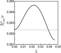
Figure 9: $\bar{\Delta}^{\rm(h)}_{\varsigma{\rm max}}$ as a function of the strength of the electronic nematicity at the optimal doping $\delta=0.15$ for $t/J=3$ and $t^{\prime}/t=1/3$.

The above equations (30) and (A19) have been calculated self-consistently, and the result of the maximal charge-carrier pair gap parameter $\bar{\Delta}^{\rm(h)}_{\varsigma{\rm max}}=\bar{\Delta}^{\rm(h)}_{\varsigma}({\bf k})|_{{\bf k}=[0,\pi]}$ in Eq. (23a) as a function of the strength of the electronic nematicity is plotted in Fig. 9, where with the increase of the strength of the electronic nematicity, $\bar{\Delta}^{\rm(h)}_{\varsigma{\rm max}}$ is raised gradually in the weak strength region, and reaches the maximum around the optimal strength of the electronic nematicity $\varsigma\approx 0.022$. However, with the further increase of the electronic nematicity, $\bar{\Delta}^{\rm(h)}_{\varsigma{\rm max}}$ then turns into a monotonically decrease in the strong strength region.

A.4 Charge-carrier pair transition temperature

The evolution of the charge-carrier pair transition temperature $T^{\rm(pair)}_{\rm c}$ with the doping concentration or the strength of the electronic nematicity can be evaluated self-consistently from the above self-consistent equations (30) and (A19) at the condition of the charge-carrier pair gap parameter $\bar{\Delta}_{\varsigma}^{\rm(h)}=0$ [then $\bar{\Delta}_{\varsigma\hat{x}}^{\rm(h)}=0$ and $\bar{\Delta}_{\varsigma\hat{y}}^{\rm(h)}=0$]. We Feng15a have shown that this $T^{\rm(pair)}_{\rm c}$ is the exactly same as that obtained from the corresponding electron pairing state at the condition of the electron pair gap parameter $\bar{\Delta}^{(\varsigma)}=0$, and will return to this discussion of $T^{\rm(pair)}_{\rm c}$ towards subsection A.7 of this Appendix. The above results thus also show that (i) the mechanism of the formation of the charge-carrier pairs is purely electronic without phonons; (ii) the mechanism indicates that the strong correlation favors the formation of the charge-carrier pairs (then the electron pairs), since the main ingredient is identified into a charge-carrier pairing mechanism not involving the phonon, the external degree of freedom, but the internal spin degree of freedom of electron; (iii) the charge-carrier pairing state is controlled by both the charge-carrier pair gap $\bar{\Delta}_{\varsigma}^{\rm(h)}({\bf k})$ and charge-carrier quasiparticle coherent weight $Z^{\rm(h)}_{\varsigma{\rm F}}$.

A.5 Full charge-spin recombination

For the discussions of the exotic features of the electronic structure of cuprate superconductors in the SC-state with coexisting electronic nematicity, we need to derive the full electron diagonal and off-diagonal propagators $G_{\varsigma}({\bf k},\omega)$ and $\Im^{\dagger}_{\varsigma}({\bf k},\omega)$ in Eq. (3) of the main text. In the previous studies for the case without rotation symmetry-breaking, we Feng15a have developed a full charge-spin recombination scheme, where a charge carrier and a localized spin are fully recombined into a constrained electron. In particular, within this full charge-spin recombination scheme, it has been realized that the coupling form between the electrons and spin excitations is the same as that between the charge carriers and spin excitations, which therefore indicates that the form of the self-consistent equations satisfied by the full electron diagonal and off-diagonal propagators is the same as the form satisfied by the full charge-carrier diagonal and off-diagonal propagators. Following these previous discussions Feng15a , we can perform a full charge-spin recombination in the present case with broken rotation symmetry in which the full charge-carrier diagonal and off-diagonal propagators $g_{\varsigma}({\bf k},\omega)$ and $\Gamma^{\dagger}_{\varsigma}({\bf k},\omega)$ in Eq. (20) are replaced by the full electron diagonal and off-diagonal propagators $G_{\varsigma}({\bf k},\omega)$ and $\Im^{\dagger}_{\varsigma}({\bf k},\omega)$, respectively, and then the self-consistent equations satisfied by the full electron diagonal and off-diagonal propagators of the $t$-$J$ model (1) in the SC-state with coexisting electronic nematicity can be obtained explicitly as,

$$G_{\varsigma}({\bf k},\omega) = G^{(0)}_{\varsigma}({\bf k},\omega)+G^{(0)}_{\varsigma}({\bf k},\omega)[\Sigma^{(\varsigma)}_{\rm ph}({\bf k},\omega)G_{\varsigma}({\bf k},\omega)$$ (32a)

$$- \Sigma^{(\varsigma)}_{\rm pp}({\bf k},\omega)\Im^{\dagger}_{\varsigma}({\bf k},\omega)],~{}$$

$$\Im^{\dagger}_{\varsigma}({\bf k},\omega) = G^{(0)}_{\varsigma}({\bf k},-\omega)[\Sigma^{(\varsigma)}_{\rm ph}({\bf k},-\omega)\Im^{\dagger}_{\varsigma}({\bf k},\omega)$$ (32b)

$$+ \Sigma^{(\varsigma)}_{\rm pp}({\bf k},\omega)G_{\varsigma}({\bf k},\omega)],$$

where $G^{(0)}_{\varsigma}({\bf k},\omega)$ is the electron diagonal propagator of the $t$-$J$ model (1) in the tight-binding approximation, and can be expressed explicitly as,

$$G^{(0)}_{\varsigma}({\bf k},\omega) = {1\over\omega-\varepsilon^{(\varsigma)}_{\bf k}},$$ (33)

while the electron normal self-energy $\Sigma^{(\varsigma)}_{\rm ph}({\bf k},\omega)$ in the particle-hole channel and electron anomalous self-energy $\Sigma^{(\varsigma)}_{\rm pp}({\bf k},\omega)$ in the particle-particle channel can be obtained directly from the corresponding parts of the charge-carrier normal self-energy $\Sigma^{(\rm h)}_{\varsigma{\rm ph}}({\bf k},\omega)$ and charge-carrier anomalous self-energy $\Sigma^{(\rm h)}_{\varsigma{\rm pp}}({\bf k},\omega)$ in Eq. (21) by the replacement of the full charge-carrier diagonal and off-diagonal propagators $g_{\varsigma}({\bf k},\omega)$ and $\Gamma^{\dagger}_{\varsigma}({\bf k},\omega)$ with the corresponding full electron diagonal and off-diagonal propagators $G_{\varsigma}({\bf k},\omega)$ and $\Im^{\dagger}_{\varsigma}({\bf k},\omega)$ as,

$$\Sigma^{(\varsigma)}_{\rm ph}({\bf k},i\omega_{n}) = {1\over N^{2}}\sum_{{\bf p},{\bf p}^{\prime}}[\Lambda^{(\varsigma)}_{{\bf p}+{\bf p}^{\prime}+{\bf k}}]^{2}$$

$$\times {1\over\beta}\sum_{ip_{m}}G_{\varsigma}({{\bf p}+{\bf k}},ip_{m}+i\omega_{n})\Pi_{\varsigma}({\bf p},{\bf p}^{\prime},ip_{m}),$$

$$\Sigma^{(\varsigma)}_{\rm pp}({\bf k},i\omega_{n}) = {1\over N^{2}}\sum_{{\bf p},{\bf p}^{\prime}}[\Lambda^{(\varsigma)}_{{\bf p}+{\bf p}^{\prime}+{\bf k}}]^{2}$$

$$\times {1\over\beta}\sum_{ip_{m}}\Im^{\dagger}_{\varsigma}({\bf p}+{\bf k},ip_{m}+i\omega_{n})\Pi_{\varsigma}({\bf p},{\bf p}^{\prime},ip_{m}),$$

respectively, and then the corresponding full electron diagonal and off-diagonal propagators now can be obtained from Eq. (32) as quoted in Eq. (3) of the main text. The above electron normal self-energy $\Sigma^{(\varsigma)}_{\rm ph}({\bf k},\omega)$ describes the electron quasiparticle coherence, and therefore gives rise to a main contribution to the energy and lifetime renormalization of the electrons, while the electron anomalous self-energy $\Sigma^{(\varsigma)}_{\rm pp}({\bf k},\omega)$ is defined as the momentum and energy dependence of the electron pair gap, $\Sigma^{(\varsigma)}_{\rm pp}({\bf k},\omega)=\bar{\Delta}^{(\varsigma)}({\bf k},\omega)=\bar{\Delta}^{(\varsigma)}_{\hat{x}}({\bf k},\omega)-\bar{\Delta}^{(\varsigma)}_{\hat{y}}({\bf k},\omega)$, and therefore is corresponding to the energy for breaking an electron pair.

In analogy to the calculation of the charge-carrier normal and anomalous self-energies in subsection A.2, we can also derive explicitly the electron normal and anomalous self-energies. Firstly, the electron normal self-energy $\Sigma^{(\varsigma)}_{\rm ph}({\bf k},\omega)$ can be separated into its symmetric and antisymmetric parts as: $\Sigma^{(\varsigma)}_{\rm ph}({\bf k},\omega)=\Sigma^{(\varsigma)}_{\rm phe}({\bf k},\omega)+\omega\Sigma^{(\varsigma)}_{\rm pho}({\bf k},\omega)$, with the corresponding symmetric part $\Sigma^{(\varsigma)}_{\rm phe}({\bf k},\omega)$ and antisymmetric part $\Sigma^{(\varsigma)}_{\rm pho}({\bf k},\omega)$ that are an even function of energy. In particular, this antisymmetric part $\Sigma^{(\varsigma)}_{\rm pho}({\bf k},\omega)$ is defined as the electron quasiparticle coherent weight as: $Z^{(\varsigma)-1}_{\rm F}({\bf k},\omega)=1-{\rm Re}\Sigma^{(\varsigma)}_{\rm pho}({\bf k},\omega)$. In an interacting electron system, everything happens at around EFS. As a case for low-energy close to EFS, the electron pair gap and electron quasiparticle coherent weight therefore can be discussed in the static-limit approximation,

$$\bar{\Delta}^{(\varsigma)}({\bf k}) = {1\over 2}[\bar{\Delta}^{(\varsigma)}_{\hat{x}}{\rm cos}k_{x}-\bar{\Delta}^{(\varsigma)}_{\hat{y}}{\rm cos}k_{y}],$$ (35a)

$${1\over Z^{(\varsigma)}_{\rm F}} = 1-{\rm Re}\Sigma^{(\varsigma)}_{\rm pho}({\bf k},\omega=0)\mid_{{\bf k}=[\pi,0]},~{}~{}~{}$$ (35b)

where the wave vector ${\bf k}$ in $Z^{(\varsigma)}_{\rm F}({\bf k})$ has been chosen as ${\bf k}=[\pi,0]$ just as it has been done in the ARPES experiments Ding01 ; DLFeng00 . Moreover, as in the case for the charge-carrier pair gap in Eq. (25), the electron pair gap in Eq. (35a) can be also expressed explicitly as,

$$\bar{\Delta}^{(\varsigma)}({\bf k})=\bar{\Delta}^{(\varsigma)}_{\rm d}\gamma^{\rm(d)}_{\bf k}+\bar{\Delta}^{(\varsigma)}_{\rm s}\gamma^{\rm(s)}_{\bf k},$$ (36)

with the d-wave component of the electron pair gap parameter $\bar{\Delta}^{(\varsigma)}_{\rm d}=(\bar{\Delta}^{(\varsigma)}_{\hat{x}}+\bar{\Delta}^{(\varsigma)}_{\hat{y}})/2$ and the s-wave component $\bar{\Delta}^{(\varsigma)}_{\rm s}=(\bar{\Delta}^{(\varsigma)}_{\hat{x}}-\bar{\Delta}^{(\varsigma)}_{\hat{y}})/2$.

With the above static-limit approximation for the electron pair gap $\bar{\Delta}^{(\varsigma)}({\bf k})$ and electron quasiparticle coherent weight $Z^{(\varsigma)}_{\rm F}$, the renormalized electron diagonal and off-diagonal propagators now can be derived directly from Eq. (32) as,

$$G^{\rm(RMF)}_{\varsigma}({\bf k},\omega) = Z^{(\varsigma)}_{\rm F}\left({U^{(\varsigma)2}_{\bf k}\over\omega-E^{(\varsigma)}_{\bf k}}+{V^{(\varsigma)2}_{\bf k}\over\omega+E^{(\varsigma)}_{\bf k}}\right),~{}~{}~{}~{}~{}~{}$$ (37a)

$$\Im^{{\rm(RMF)}\dagger}_{\varsigma}({\bf k},\omega) = -Z^{(\varsigma)}_{\rm F}{\bar{\Delta}^{(\varsigma)}_{\rm Z}({\bf k})\over 2E^{(\varsigma)}_{\bf k}}\left({1\over\omega-E^{(\varsigma)}_{\bf k}}\right.$$ (37b)

$$- \left.{1\over\omega+E^{(\varsigma)}_{\bf k}}\right),$$

where the renormalized electron orthorhombic energy dispersion $\bar{\varepsilon}^{(\varsigma)}_{\bf k}=Z^{(\varsigma)}_{\rm F}\varepsilon^{(\varsigma)}_{\bf k}$, the renormalized electron pair gap $\bar{\Delta}^{(\varsigma)}_{\rm Z}({\bf k})=Z^{(\varsigma)}_{\rm F}\bar{\Delta}^{(\varsigma)}({\bf k})$, the SC quasiparticle energy spectrum $E^{(\varsigma)}_{\bf k}=\sqrt{\bar{\varepsilon}^{(\varsigma)2}_{\bf k}+|\bar{\Delta}^{(\varsigma)}_{\rm Z}({\bf k})|^{2}}$, and the SC quasiparticle coherence factors

$$U^{(\varsigma)2}_{\bf k} = {1\over 2}\left(1+{\bar{\varepsilon}^{(\varsigma)}_{\bf k}\over E^{(\varsigma)}_{\bf k}}\right),$$ (38a)

$$V^{(\varsigma)2}_{\bf k} = {1\over 2}\left(1-{\bar{\varepsilon}^{(\varsigma)}_{\bf k}\over E^{(\varsigma)}_{\bf k}}\right),$$ (38b)

with the constraint $U^{(\varsigma)2}_{\bf k}+V^{(\varsigma)2}_{\bf k}=1$ for any wave vector ${\bf k}$. The above result in Eq. (36) therefore show that the symmetry of superconductivity with coexisting electronic nematicity is modified from the ordinary d-wave electron pairing to the d+s wave Kitatani17 ; Maier14 . Moreover, the results in Eqs. (37) and (38) are the standard Bardeen-Cooper-Schrieffer expressions for an electron pair state Schrieffer64 , although the electron pairing mechanism is driven by the kinetic energy by the exchange of a strongly dispersive spin excitation.

Substituting these renormalized electron diagonal and off-diagonal propagators in Eq. (37) and MF spin propagator in Eq. (17a) into Eqs. (34), the electron normal and anomalous self-energies can be obtained explicitly as,

$${\Sigma}^{(\varsigma)}_{\rm ph}({\bf{k}},{\omega}) = \frac{1}{N^{2}}\sum_{{\bf{p}}{\bf{p}^{\prime}}{\nu}}(-1)^{\nu+1}{\Omega}^{(\varsigma)}_{{\bf{p}}{\bf{p}^{\prime}}{\bf{k}}}\left[U^{(\varsigma)2}_{\bf{p}+\bf{k}}\left(\frac{F^{(\varsigma)}_{1\nu}({\bf p},{\bf p}^{\prime},{\bf k})}{\omega+\omega^{(\nu)}_{\varsigma{\bf{p}}{\bf{p}}^{\prime}}-E^{(\varsigma)}_{\bf{p}+\bf{k}}}-\frac{F^{(\varsigma)}_{2\nu}({\bf p},{\bf p}^{\prime},{\bf k})}{\omega-\omega^{(\nu)}_{\varsigma{\bf{p}}{\bf{p}}^{\prime}}-E^{(\varsigma)}_{\bf{p}+\bf{k}}}\right)\right.$$ (39a)

$$+ \left.V^{(\varsigma)2}_{\bf{p}+\bf{k}}\left(\frac{F^{(\varsigma)}_{1\nu}({\bf p},{\bf p}^{\prime},{\bf k})}{\omega-\omega^{(\nu)}_{\varsigma{\bf{p}}{\bf{p}}^{\prime}}+E^{(\varsigma)}_{\bf{p}+\bf{k}}}-\frac{F^{(\varsigma)}_{2\nu}({\bf p},{\bf p}^{\prime},{\bf k})}{\omega+\omega^{(\nu)}_{\varsigma{\bf{p}}{\bf{p}}^{\prime}}+E^{(\varsigma)}_{\bf{p}+\bf{k}}}\right)\right],$$

$${\Sigma}^{(\varsigma)}_{\rm pp}({\bf{k}},{\omega}) = \frac{1}{N^{2}}\sum_{{\bf{p}}{\bf{p}^{\prime}}{\nu}}(-1)^{\nu}{\Omega}^{(\varsigma)}_{{\bf{p}}{\bf{p}^{\prime}}{\bf{k}}}\frac{\bar{\Delta}_{\varsigma{\rm{Z}}}({\bf{p}}+{\bf{k}})}{2E^{(\varsigma)}_{{\bf{p}}+\bf{k}}}\left[\left(\frac{F^{(\varsigma)}_{1\nu}({\bf p},{\bf p}^{\prime},{\bf k})}{\omega+\omega^{(\nu)}_{\varsigma{\bf{p}}{\bf{p}}^{\prime}}-E^{(\varsigma)}_{\bf{p}+\bf{k}}}-\frac{F^{(\varsigma)}_{2\nu}({\bf p},{\bf p}^{\prime},{\bf k})}{\omega-\omega^{(\nu)}_{\varsigma{\bf{p}}{\bf{p}}^{\prime}}-E^{(\varsigma)}_{\bf{p}+\bf{k}}}\right)\right.$$ (39b)

$$- \left.\left(\frac{F^{(\varsigma)}_{1\nu}({\bf p},{\bf p}^{\prime},{\bf k})}{\omega-\omega^{(\nu)}_{\varsigma{\bf{p}}{\bf{p}}^{\prime}}+E^{(\varsigma)}_{\bf{p}+\bf{k}}}-\frac{F^{(\varsigma)}_{2\nu}({\bf p},{\bf p}^{\prime},{\bf{k}})}{\omega+\omega^{(\nu)}_{\varsigma{\bf{p}}{\bf{p}}^{\prime}}+E^{(\varsigma)}_{\bf{p}+\bf{k}}}\right)\right],$$

respectively, where $\nu=1,2$, ${\Omega}^{(\varsigma)}_{{\bf{p}}{\bf{p}^{\prime}}{\bf{k}}}=Z^{(\varsigma)}_{\rm{F}}[\Lambda^{(\varsigma)}_{{\bf{p}}+{\bf{p}^{\prime}}+{\bf{k}}}]^{2}B^{(\varsigma)}_{\bf{p}^{\prime}}B^{(\varsigma)}_{\bf{p}+\bf{p}^{\prime}}/(4\omega^{(\varsigma)}_{\bf{p}^{\prime}}\omega^{(\varsigma)}_{\bf{p}+\bf{p}^{\prime}})$, and the functions,

$$F^{(\varsigma)}_{1\nu}({\bf{p}},{\bf{p}}^{\prime},{\bf{k}}) = n_{\rm{F}}(E^{(\varsigma)}_{\bf{p}+\bf{k}})\{1+n_{B}(\omega^{(\varsigma)}_{\bf{p}^{\prime}+\bf{p}})+n_{B}[(-1)^{\nu+1}\omega^{(\varsigma)}_{\bf{p}^{\prime}}]\}+n_{B}(\omega^{(\varsigma)}_{\bf{p}^{\prime}+\bf{p}})n_{B}[(-1)^{\nu+1}\omega^{(\varsigma)}_{\bf{p}^{\prime}}],$$ (40a)

$$F^{(\varsigma)}_{2\nu}({\bf{p}},{\bf{p}}^{\prime},{\bf{k}}) = [1-n_{\rm{F}}(E^{(\varsigma)}_{\bf{p}+\bf{k}})]\{1+n_{B}(\omega^{(\varsigma)}_{\bf{p}^{\prime}+\bf{p}})+n_{B}[(-1)^{\nu+1}\omega^{(\varsigma)}_{\bf{p}^{\prime}}]\}+n_{B}(\omega^{(\varsigma)}_{\bf{p}^{\prime}+\bf{p}})n_{B}[(-1)^{\nu+1}\omega^{(\varsigma)}_{\bf{p}^{\prime}}].~{}~{}~{}~{}$$ (40b)

A.6 Self-consistent equations for determination of electron order parameters

The above electron quasiparticle coherent weight, two components of the electron pair gap parameter, and the electron chemical potential satisfy following four self-consistent equations,

$$\frac{1}{Z^{(\varsigma)}_{\rm{F}}} = 1+\frac{1}{N^{2}}\sum_{{\bf{p}}{\bf{p}^{\prime}}{\nu}}(-1)^{\nu+1}\Omega^{(\varsigma)}_{{\bf{p}}{\bf{p}^{\prime}}{\bf k}_{\rm A}}\left(\frac{F^{(\varsigma)}_{1\nu}({\bf p},{\bf p}^{\prime},{\bf k}_{\rm A})}{(\omega^{(\nu)}_{\varsigma{\bf{p}}{\bf{p}}^{\prime}}-E^{(\varsigma)}_{\bf{p}+{\bf k}_{\rm A}})^{2}}+\frac{F^{(\varsigma)}_{2\nu}({\bf{p}},{\bf{p}}^{\prime},{\bf k}_{\rm A})}{(\omega^{(\nu)}_{\varsigma{\bf{p}}{\bf{p}}^{\prime}}+E^{(\varsigma)}_{\bf{p}+{\bf k}_{\rm A}})^{2}}\right),$$ (41a)

$$\bar{\Delta}^{(\varsigma)}_{\hat{x}} = \frac{8}{N^{3}}\sum_{{\bf{p}}{\bf{p}^{\prime}}{\bf{k}}{\nu}}(-1)^{\nu}Z^{(\varsigma)}_{\rm{F}}\Omega^{(\varsigma)}_{{\bf{p}}{\bf{p}^{\prime}}{\bf{k}}}\frac{\gamma_{{\bf k}_{x}}(\bar{\Delta}^{(\varsigma)}_{\hat{x}}\gamma_{{\bf p}_{x}+{\bf k}_{x}}-\bar{\Delta}^{(\varsigma)}_{\hat{y}}\gamma_{{\bf p}_{y}+{\bf k}_{y}})}{E^{(\varsigma)}_{\bf{p}+\bf{k}}}\left(\frac{F^{(\varsigma)}_{1\nu}({\bf{p}},{\bf{p}}^{\prime},{\bf{k}})}{\omega^{(\nu)}_{\varsigma{\bf{p}}{\bf{p}}^{\prime}}-E^{(\varsigma)}_{\bf{p}+\bf{k}}}-\frac{F^{(\varsigma)}_{2\nu}({\bf{p}},{\bf{p}}^{\prime},{\bf{k}})}{\omega^{(\nu)}_{\varsigma{\bf{p}}{\bf{p}}^{\prime}}+E^{(\varsigma)}_{\bf{p}+\bf{k}}}\right),~{}~{}~{}~{}~{}$$ (41b)

$$\bar{\Delta}^{(\varsigma)}_{\hat{y}} = \frac{8}{N^{3}}\sum_{{\bf{p}}{\bf{p}^{\prime}}{\bf{k}}{\nu}}(-1)^{\nu+1}Z^{(\varsigma)}_{\rm{F}}\Omega^{(\varsigma)}_{{\bf{p}}{\bf{p}^{\prime}}{\bf{k}}}\frac{\gamma_{{\bf k}_{y}}(\bar{\Delta}^{(\varsigma)}_{\hat{x}}\gamma_{{\bf p}_{x}+{\bf k}_{x}}-\bar{\Delta}^{(\varsigma)}_{\hat{y}}\gamma_{{\bf p}_{y}+{\bf k}_{y}})}{E^{(\varsigma)}_{\bf{p}+\bf{k}}}\left(\frac{F^{(\varsigma)}_{1\nu}({\bf{p}},{\bf{p}}^{\prime},{\bf{k}})}{\omega^{(\nu)}_{\varsigma{\bf{p}}{\bf{p}}^{\prime}}-E^{(\varsigma)}_{\bf{p}+\bf{k}}}-\frac{F^{(\varsigma)}_{2\nu}({\bf{p}},{\bf{p}}^{\prime},{\bf{k}})}{\omega^{(\nu)}_{\varsigma{\bf{p}}{\bf{p}}^{\prime}}+E^{(\varsigma)}_{\bf{p}+\bf{k}}}\right),~{}~{}~{}~{}~{}$$ (41c)

$$1-\delta = \frac{1}{2N}\sum_{{\bf{k}}}Z^{(\varsigma)}_{\rm{F}}\left(1-\frac{\bar{\varepsilon}^{(\varsigma)}_{\bf{k}}}{E^{(\varsigma)}_{{\bf{k}}}}{\rm{tanh}}\left[\frac{1}{2}\beta{E^{(\varsigma)}_{\bf{k}}}\right]\right),$$ (41d)

where ${\bf k}_{\rm A}=[\pi,0]$. In the same calculation condition as in the evaluation of the self-consistent equations (30) and (A19), the above self-consistent equations (41) have been also solved simultaneously, and then the electron quasiparticle coherent weight, two components of the electron pair gap parameter, and electron chemical potential are obtained without using any adjustable parameters. In particular, the dome-like shape nematic-order strength dependence of $\bar{\Delta}^{\rm(h)}_{\varsigma{\rm max}}$ shown in Fig. 9 therefore also leads to the same dome-like shape nematic-order strength dependence of $\bar{\Delta}^{(\varsigma)}_{\rm max}$ in Eq. (35a). Moreover, it should be emphasized that the self-consistent equation in Eq. (41d) guarantees that the EFS contour in the presence of the electronic nematicity still satisfy Luttinger’s theorem Luttinger60 , i.e., the effective area of the EFS contour contains $1-\delta$ electrons.

A.7 Electron pair transition temperature

Concomitantly, the evolution of the electron pair transition temperature $T_{\rm c}$ with the doping or the strength of the electronic nematicity can be obtained self-consistently from the above self-consistent equations in Eq. (41) at the condition of the electron pair gap parameter $\bar{\Delta}^{(\varsigma)}=0$ [then $\bar{\Delta}^{(\varsigma)}_{\hat{x}}=0$ and $\bar{\Delta}^{(\varsigma)}_{\hat{y}}=0$].

In our previous study Feng15a , it has been demonstrated that in a given doping concentration, the magnitude of the electron pair transition temperature $T_{\rm c}$ obtained from the electron pairing state is the exactly same as the magnitude of the charge-carrier pair transition temperature $T^{\rm(pair)}_{\rm c}$ obtained from the corresponding charge-carrier pairing state. Within the framework of the kinetic-energy-driven superconductivity Feng15 ; Feng0306 ; Feng12 ; Feng15a , the effective attractive interaction between charge carriers originates in their coupling to a strongly dispersive spin excitation, while the electron pairing interaction in the full charge-spin recombination scheme Feng15a is mediated by the same spin excitation, which therefore leads to that the electron pair transition temperature $T_{\rm c}$ is identical to the charge-carrier pair transition-temperature $T^{\rm(pair)}_{\rm c}$, and then the dome-like shape of the doping dependence of $T_{\rm c}$ with its maximum occurring at around the optimal doping is a natural consequence of the dome-like shape of the doping dependence of $T^{\rm(pair)}_{\rm c}$ with its maximum occurring at around the same optimal doping.

In the SC-state with coexisting electronic nematicity, our present results therefore show that the value of $T_{\rm c}$ obtained self-consistently from the equations (41) also is the exactly same as the corresponding value of $T^{\rm(pair)}_{\rm c}$ obtained self-consistently in subsection A.4 of this Appendix from the equations (30) and (A19) in a given doping concentration and strength of the electronic nematicity, and then the dome-like shape nematic-order strength dependence of the optimized $T_{\rm c}$ with its maximum appearing at around the optimal strength of the electronic nematicity also is a natural consequence of the dome-like shape nematic-order strength dependence of the optimized $T^{\rm(pair)}_{\rm c}$ with its maximum appearing at around the same optimal doping.

References

- (1) J. G. Bednorz and K. A. Müller, Possible High Superconductivity in the Ba-La-Cu-O System, Z. Phys. B 64 (1986), pp. 189–193.
- (2) M. K. Wu, J. R. Ashburn, C. J. Torng, P. H. Hor, R. L. Meng, L. Gao, Z. J. Huang, Y. Q. Wang, and C. W. Chu, Superconductivity at 93 K in a New Mixed-Phase Y-Ba-Cu-O Compound System at Ambient Pressure, Phys. Rev. Lett. 58 (1987), pp. 908–910.
- (3) See, e.g., the review, M. Fujita, H. Hiraka, M. Matsuda, M. Matsuura, J. M. Tranquada, S. Wakimoto, G. Xu, and K. Yamada, Progress in Neutron Scattering Studies of Spin Excitations in High- Cuprates, J. Phys. Soc. Jpn. 81 (2012), pp. 011007-1–011007-19.
- (4) P. W. Anderson, The Resonating Valence Bond State in and Superconductivity, Science 235 (1987), pp. 1196–1198.
- (5) See, e.g., the review, T. Timusk and B. Statt, The pseudogap in high-temperature superconductors: an experimental survey, Rep. Prog. Phys. 62 (1999), pp. 61–122.
- (6) See, e.g., the review, S. Hüfner, M. A. Hossain, A. Damascelli, and G. A. Sawatzky, Two Gaps Make a High-Temperature Superconductor?, Rep. Prog. Phys. 71 (2008), pp. 062501-1–062501-9.
- (7) See, e.g., the review, I. M. Vishik, Photoemission perspective on pseudogap, superconducting fluctuations, and charge order incuprates: a review of recent progress, Rep. Prog. Phys. 81 (2018), pp. 062501-1–062501-10.
- (8) See, e.g., the review, R. Comin and A. Damascelli, Resonant x-ray scattering studies of charge order in cuprates, Annu. Rev. Condens. Matter Phys. 7 (2016), pp. 369–405.
- (9) Matthias Vojta, Lattice symmetry breaking in cuprate superconductors: Stripes, nematics, and superconductivity, Adv. Phys. 58 (2009), pp. 699–820.
- (10) E. Fradkin, S. A. Kivelson, M. J. Lawler, J. P. Eisenstein, and A. P. Mackenzie, Nematic Fermi Fluids in Condensed Matter Physics, Annu. Rev. Condens. Matter Phys. 1 (2010), pp. 153–178.
- (11) R. M. Fernandes, P. P. Orth, and J. Schmalian, Intertwined vestigial order in quantum materials: nematicity and beyond, Annu. Rev. Condens. Matter Phys. 10 (2019), pp. 133–154.
- (12) M. J. Lawler, K. Fujita, J. Lee, A. R. Schmidt, Y. Kohsaka, C. K. Kim, H. Eisaki, S. Uchida, J. C. Davis, J. P. Sethna, and E.-A. Kim, Intra-unit-cell electronic nematicity of the high- copper-oxide pseudogap states, Nature 466 (2010), pp. 347–351.
- (13) K. Fujita, C. K. Kim, I. Lee, J. Lee, M. H. Hamidian, I. A. Firmo, S. Mukhopadhyay, H. Eisaki, S. Uchida, M. J. Lawler, E.-A. Kim, J. C. Davis, Simultaneous Transitions in Cuprate Momentum-Space Topology and Electronic Symmetry Breaking, Science 344 (2014), pp. 612–616.
- (14) Y. Zheng, Y. Fei, K. Bu, W. Zhang, Y. Ding, X. J. Zhou, J. E. Hoffman, and Y. Yin, The study of electronic nematicity in an overdoped superconductor using scanning tunneling spectroscopy, Sci. Rep. 7 (2017), pp. 8059-1–80598.
- (15) S. Mukhopadhyay, R. Sharma, C. K. Kim, S. D. Edkins, M. H. Hamidian, H. Eisaki, S. Uchida, E.-A. Kim, M. J. Lawler, A. P. Mackenzie, J. C. S. Davis, and K. Fujita, Evidence for a vestigial nematic state in the cuprate pseudogap phase, Proc. Natl. Acad. Sci. 116 (2019), pp. 13249–13254; S. A. Kivelson and S. Lederer, Linking the pseudogap in the cuprates with local symmetry breaking: A commentary, Proc. Natl. Acad. Sci. 116 (2019), pp. 14395-14396.
- (16) S. Nakata, M. Horio, K. Koshiishi, K. Hagiwara, C. Lin, M. Suzuki, S. Ideta, K. Tanaka, D. Song, Y. Yoshida, H. Eisaki, A. Fujimori, Nematicity in the pseudogap state of cuprate superconductors revealed by angle-resolved photoemission spectroscopy, npj Quantum Mater. 6 (2021), pp. 86-1–86-5.
- (17) V. Hinkov, D. Haug, B. Fauqué, P. Bourges, Y. Sidis, A. Ivanov, C. Bernhard, C. T. Lin, B. Keimer, Electronic Liquid Crystal State in the High-Temperature Superconductor , Science 319 (2008), pp. 597–600.
- (18) Y. Sato, S. Kasahara, H. Murayama, Y. Kasahara, E.-G. Moon, T. Nishizaki, T. Loew, J. Porras, B. Keimer, T. Shibauchi, and Y. Matsuda, Thermodynamic evidence for a nematic phase transition at the onset of the pseudogap in , Nat. Phys. 13 (2017), pp. 1074–1078.
- (19) R. Daou, J. Chang, D. LeBoeuf, O. Cyr-Choiniére, F. Laliberté, N. Doiron-Leyraud, B. J. Ramshaw, R. Liang, D. A. Bonn, W. N. Hardy, and L. Taillefer, Broken rotational symmetry in the pseudogap phase of a high- superconductor, Nature 463 (2010), pp. 519–522.
- (20) O. Cyr-Choiniére, G. Grissonnanche, S. Badoux, J. Day, D. A. Bonn, W. N. Hardy, R. Liang, N. Doiron-Leyraud, and L. Taillefer, Two types of nematicity in the phase diagram of the cuprate superconductor , Phys. Rev. B 92 (2015), pp. 224502-1–224502-7.
- (21) W. Wang, J. Luo, C. G. Wang, J. Yang, Y. Kodama, R. Zhou, G.-Q Zheng, Microscopic evidence for the intra-unit-cell electronic nematicity inside the pseudogap phase in , Sci. China-Phys. Mech. Astron. 64 (2021), pp. 237413-1–237413-6.
- (22) Y. Ando, K. Segawa, S. Komiya, and A. N. Lavrov, Electrical Resistivity Anisotropy from Self-Organized One-Dimensionality in High-Temperature Superconductors, Phys. Rev. Lett. 88 (2002), pp. 137005-1–137005-4.
- (23) J. Wu, A. T. Bollinger, X. He, and I. Boz̃ović, Spontaneous breaking of rotational symmetry in copper oxide superconductors, Nature 547 (2017), pp. 432–435.
- (24) N. Auvray, B. Loret, S. Benhabib, M. Cazayous, R. D. Zhong, J. Schneeloch, G. D. Gu, A. Forget, D. Colson, I. Paul, A. Sacuto, and Y. Gallais, Nematic fluctuations in the cuprate superconductor , Nat. Commun. 10 (2019), p. 5209-1–5209-7.
- (25) S. A. Kivelson, E. Fradkin, and V. J. Emery, Electronic Liquid Crystal Phases of a Doped Mott Insulator, Nature 393 (1998), pp. 550–553.
- (26) J. Zaanen, Quantum phase transitions in cuprates: stripes and antiferromagnetic supersolids, Physica C 317-318 (1999), pp. 217–229.
- (27) S. A. Kivelson, I. P. Bindloss, E. Fradkin, V. Oganesyan, J. M. Tranquada, A. Kapitulnik, and C. Howald, How to detect fluctuating stripes in the high-temperature superconductors, Rev. Mod. Phys. 75 (2003), pp. 1201–1241.
- (28) L. Nie, L. E. H. Sierens, R. G. Melko, S. Sachdev, and S. A. Kivelson, Fluctuating orders and quenched randomness in the cuprates, Phys. Rev. B 92 (2015), pp. 174505-1–174505-13.
- (29) C. J. Halboth and W. Metzner, d-wave superconductivity and Pomeranchuk instability in the two-dimensional Hubbard model, Phys. Rev. Lett. 85 (2000), pp. 5162–5165.
- (30) S. Okamoto, D. Sénéchal, M. Civelli, and A.-M. S. Tremblay, Dynamical electronic nematicity from Mott physics, Phys. Rev. B 82 (2010), pp. 180511-1–180511-4.
- (31) M. Kitatani, N. Tsuji, and H. Aoki, Interplay of Pomeranchuk instability and superconductivity in the two-dimensional repulsive Hubbard model, Phys. Rev. B 95 (2017), pp. 075109-1–075109-7.
- (32) Z. Dai, Y.-H. Zhang, T. Senthil, and P. A. Lee, Pair density wave, charge density wave and vortices in high cuprates, Phys. Rev. B 97 (2018), pp. 174511-1–174511-19.
- (33) W. L. Tu and T. K. Lee, Evolution of Pairing Orders between Pseudogap and Superconducting Phases of Cuprate Superconductors, Sci. Rep. 9 (2019), pp. 1719-1–1719-13.
- (34) A. Miyanaga and H. Yamase, Orientational symmetry-breaking correlations in square lattice t-J model, Phys. Rev. B 73 (2006), pp. 174513-1–174513-5.
- (35) B. Edegger, V. N. Muthukumar, and C. Gros, Spontaneous breaking of the Fermi-surface symmetry in the t-J model: a numerical study, Phys. Rev. B 74 (2006), pp. 165109-1–165109-6.
- (36) A. Wollny and M. Vojta, Photoemission signatures of valence-bond stripes in cuprates: Long-range vs. short-range order, Physica B 404 (2009), pp. 3079–3084.
- (37) K. Lee, S. A. Kivelson, and E.-A. Kim, Cold-spots and glassy nematicity in underdoped cuprates, Phys. Rev. B 94 (2016), pp. 014204-1–014204-8.
- (38) T. A. Maier and D. J. Scalapino, Pairing interaction near a nematic quantum critical point of a three-band CuO2 model, Phys. Rev. B 90 (2014), pp. 174510-1–174510-5.
- (39) S. Lederer, Y. Schattner, E. Berg, and S. A. Kivelson, Enhancement of superconductivity near a nematic quantum critical point, Phys. Rev. Lett. 114 (2015), pp. 097001-1–097001-6.
- (40) J. Kaczmarczyk, T. Schickling, and J. Bünemann, Coexistence of Nematic Order and Superconductivity in the Hubbard Model, Phys. Rev. B 94 (2016), pp. 085152-1–085152-6.
- (41) S. Lederer, Y. Schattner, E. Berg, and S. A. Kivelson, Superconductivity and non-Fermi liquid behavior near a nematic quantum critical point, Proc. Natl. Acad. Sci. 114 (2017), pp. 4905–4910.
- (42) S. Feng, D. Gao and H. Zhao, Charge order driven by Fermi-arc instability and its connection with pseudogap in cuprate superconductors, Phil. Mag. 96 (2016), pp. 1245–1262; H. Zhao, D. Gao, and S. Feng, Pseudogap-generated a coexistence of Fermi arcs and Fermi pockets in cuprate superconductors, Physica C 534 (2017), pp. 1-8.
- (43) D. Gao, Y. Liu, H. Zhao, Y. Mou, and S. Feng, Interplay between charge order and superconductivity in cuprate superconductors, Physica C 551 (2018), pp. 72–81; S. Feng, D. Gao, Y. Liu, Y. Mou, and S. Tan, Hidden Pair-Density-Wave Order in Cuprate Superconductors, J. Supercond. Nov. Magn. 32 (2019), pp. 2745–2749.
- (44) L. Zhang, J. K. Jain, and V. J. Emery, Importance of the local constraint in slave-boson theories, Phys. Rev. B 47 (1993), pp. 3368–3373.
- (45) See, e.g., the review, B. Edegger, V. N. Muthukumar, and C. Gros, GutzwillerRVB theory of high-temperature superconductivity: Results from renormalized mean-field theory and variational Monte Carlo calculations, Adv. Phys.56 (2007), pp. 927–1033.
- (46) S. Feng, J. Qin, and T. Ma, A gauge invariant dressed holon and spinon description of the normal-state of underdoped cuprates, J. Phys.: Condens. Matter 16 (2004), pp. 343-359; S. Feng, Z. B. Su, and L. Yu, Fermion-Spin Transformation to Implement the Charge-Spin Separation, Phys. Rev. B 49 (1994), pp. 2368–2384.
- (47) See, e.g., the review, S. Feng, Y. Lan, H. Zhao, L. Kuang, L. Qin, and X. Ma, Kinetic-energy driven superconductivity in cuprate superconductors, Int. J. Mod. Phys. B 29 (2015), pp. 1530009-1–1530009-93.
- (48) S. Feng,Kinetic energy driven superconductivity in doped cuprates, Phys. Rev. B 68 (2003), PP. 184501-1-184501-7; S. Feng, T. Ma, and H. Guo, Magnetic nature of superconductivity in doped cuprates, Physica C 436 (2006), pp. 14–24.
- (49) S. Feng, H. Zhao, and Z. Huang, Two gaps with one energy scale in cuprate superconductors, Phys. Rev. B. 85 (2012), pp. 054509-1–054509-7; Phys. Rev. B 85 (2012), p. 099902(E).
- (50) S. Feng, L. Kuang, and H. Zhao, Electronic structure of cuprate superconductors in a full charge-spin recombination scheme, Physica C 517 (2015), pp. 5–15.
- (51) See, e.g., the review, A. Damascelli, Z. Hussain, and Z.-X. Shen, Angle-resolved photoemission studies of the cuprate superconductors, Rev. Mod. Phys. 75 (2003), pp. 473–571.
- (52) See, e.g., the review, J. C. Campuzano, M. R. Norman, M. Randeira, Photoemission in the High- Superconductors, in Physics of Superconductors, vol. II, edited by K. H. Bennemann and J. B. Ketterson (Springer, Berlin Heidelberg New York, 2004), pp. 167-273.
- (53) See, e.g., the review, J. Fink, S. Borisenko, A. Kordyuk, A. Koitzsch, J. Geck, V. Zabalotnyy, M. Knupfer, B. Buechner, and H. Berger, Dressing of the Charge Carriers in High- Superconductors, in Lecture Notes in Physics, vol. 715, edited by S. Hüfner (Springer-Verlag Berlin Heidelberg, 2007), pp. 295-325.
- (54) See, e.g., the review, X. J. Zhou, S. He, G. Liu, L. Zhao, L. Yu, and W. Zhang, New developments in laser-based photoemission spectroscopy and its scientific applications: a key issues review, Rep. Prog. Phys. 81 (2018), pp. 062101-1–062101-28.
- (55) T. Wu, H. Mayaffre, S. Krämer, M. Horvatić, C. Berthier, W. N. Hardy, R. Liang, D. A. Bonn, and M.-H. Julien, Magnetic-field-induced charge-stripe order in the high temperature superconductor , Nature 477 (2011), pp. 191–194.
- (56) G. Ghiringhelli, M. Le Tacon, M. Minola, S. Blanco-Canosa, C. Mazzoli, N. B. Brookes, G. M. De Luca, A. Frano, D. G. Hawthorn, F. He, T. Loew, M. Moretti Sala, D. C. Peets, M. Salluzzo, E. Schierle, R. Sutarto, G. A. Sawatzky, E. Weschke, B. Keimer, and L. Braicovich, Long-range incommensurate charge fluctuations in , Science 337 (2012), pp. 821–825.
- (57) R. Comin, A. Frano, M. M. Yee, Y. Yoshida, H. Eisaki, E. Schierle, E. Weschke, R. Sutarto, F. He, A. Soumyanarayanan, Y. He, M. Le Tacon, I. S. Elfimov, J. E. Hoffman, G. A. Sawatzky, B. Keimer and A. Damascelli, Charge order driven by Fermi-arc instability in , Science 343 (2014), pp. 390–392.
- (58) E. H. da Silva Neto, P. Aynajian, A. Frano, R. Comin, E. Schierle, E. Weschke, A. Gyenis, J. Wen, J. Schneeloch, Z. Xu, S. Ono, G. Gu, M. Le Tacon, and A. Yazdani, Ubiquitous Interplay between Charge Ordering and High-Temperature Superconductivity in Cuprates, Science 343 (2014), pp. 393–396.
- (59) T. P. Croft, C. Lester, M. S. Senn, A. Bombardi, and S. M. Hayden, Charge density wave fluctuations in and their competition with superconductivity, Phys. Rev. B 89 (2014), pp. 224513-1–224513-8.
- (60) M. Hücker, N. B. Christensen, A. T. Holmes, E. Blackburn, E. M. Forgan, Ruixing Liang, D. A. Bonn, W. N. Hardy, O. Gutowski, M. V. Zimmermann, S. M. Hayden, and J. Chang, Competing charge, spin, and superconducting orders in underdoped , Phys. Rev. B 90 (2014), pp. 054514-1–054514-11.
- (61) G. Campi, A. Bianconi, N. Poccia, G. Bianconi, L. Barba, G. Arrighetti, D. Innocenti, J. Karpinski, N. D. Zhigadlo, S. M. Kazakov, M. Burghammer, M. v. Zimmermann, M. Sprung and A. Ricci, Inhomogeneity of charge-density-wave order and quenched disorder in a high-Tc superconductor, Nature 525 (2015), pp. 359–362.
- (62) R. Comin, R. Sutarto, F. He, E. H. da Silva Neto, L. Chauviere, A. Fraño, R. Liang, W. N. Hardy, D. A. Bonn, Y. Yoshida, H. Eisaki, A. J. Achkar, D. G. Hawthorn, B. Keimer, G. A. Sawatzky, and A. Damascelli, The symmetry of charge order in cuprates, Nat. Mater. 14 (2015), pp. 796–800.
- (63) Y. Y. Peng, M. Salluzzo, X. Sun, A. Ponti, D. Betto, A. M. Ferretti, F. Fumagalli, K. Kummer, M. Le Tacon, X. J. Zhou, N. B. Brookes, L. Braicovich, and G. Ghiringhelli, Direct observation of charge order in underdoped and optimally doped by resonant inelastic x-ray scattering, Phys. Rev. B 94 (2016), pp. 184511-1–184511-8.
- (64) I. K. Drozdov, I. Pletikosić, C. -K. Kim, K. Fujita, G. D. Gu, J. C. S. Davis, P. D. Johnson, I. Boz̃ović, and T. Valla, Phase diagram of Bi2Sr2CaCu2O8+δ revisited, Nat. Commun. 9 (2018), pp. 5210-1-5210-7.
- (65) Z. Cao, X. Ma, H. Guo, and S. Feng, unpublished.
- (66) H. Zhao, L. Kuang, and S. Feng, Doping dependence of thermodynamic properties in cuprate superconductors, Physica C 478 (2012), pp. 49–55.
- (67) Z. Cao, X. Ma, Y. Liu, H. Guo, and S. Feng, Nematic-order state characteristic energy and its connection to enhancement of superconductivity in cuprate superconductors, arXiv:2109.10079.
- (68) R. Comin, R. Sutarto, E. H. da Silva Neto, L. Chauviere, R. Liang, W. N. Hardy, D. A. Bonn, F. He, G. A. Sawatzky, A. Damascelli, Broken translational and rotational symmetry via charge stripe order in underdoped , Science 347 (2015), pp. 1335–1339.
- (69) Z. Zhang, R. Sutarto, F. He, F. C. Chou, L. Udby, S. L. Holm, Z. H. Zhu, W. A. Hines, J. I. Budnick, and B. O. Wells, Nematicity and Charge Order in Superoxygenated , Phys. Rev. Lett. 121 (2018), pp. 067602-1–067602-5.
- (70) Q.-H. Wang and D.-H. Lee, Quasiparticle Scattering Interference in High Temperature Superconductors, Phys. Rev. B 67 (2003), pp. 020511-1–020511-4.
- (71) D. Gao, Y. Mou, Y. Liu, S. Tan, and S. Feng, Autocorrelation of quasiparticle spectral intensities and its connection with quasiparticle scattering interference in cuprate superconductors, Phil. Mag. 99 (2019), pp. 752–769.
- (72) U. Chatterjee, M. Shi, A. Kaminski, A. Kanigel, H. M. Fretwell, K. Terashima, T. Takahashi, S. Rosenkranz, Z. Z. Li, H. Raffy, A. Santander-Syro, K. Kadowaki, M. R. Norman, M. Randeria, and J. C. Campuzano, Nondispersive Fermi Arcs and the Absence of Charge Ordering in the Pseudogap Phase of , Phys. Rev. Lett. 96 (2006), pp. 107006-1–107006-4.
- (73) Y. He, Y. Yin, M. Zech, A. Soumyanarayanan, M. M. Yee, T. Williams, M. C. Boyer, K. Chatterjee, W. D. Wise, I. Zeljkovic, T. Kondo, T. Takeuchi, H. Ikuta, P. Mistark, R. S. Markiewicz, A. Bansil, S. Sachdev, E. W. Hudson, J. E. Hoffman, Fermi Surface and Pseudogap Evolution in a Cuprate Superconductor, Science 344 (2014), pp. 608–611.
- (74) W. Kohn and D. Sherrington, Two Kinds of Bosons and Bose Condensates, Rev. Mod. Phys. 42 (1970), pp. 1–11.
- (75) J. P. Hinton, E. Thewalt, Z. Alpichshev, F. Mahmood, J. D. Koralek, M. K. Chan, M. J. Veit, C. J. Dorow, N. Barišić, A. F. Kemper, D. A. Bonn, W. N. Hardy, R. Liang, N. Gedik, M. Greven, A. Lanzara, and J. Orenstein, The rate of quasiparticle recombination probes the onset of coherence in cuprate superconductors, Sci. Rep. 6, (2016), pp. 23610-1–23610-9
- (76) I. M. Vishik, E. A. Nowadnick, W. S. Lee, Z. X. Shen, B. Moritz, T. P. Devereaux, K. Tanaka, T. Sasagawa, and T. Fujii, A momentum-dependent perspective on quasiparticle interference in , Nat. Phys. 5, (2009), pp. 718–721.
- (77) D. S. Dessau, B. O. Wells, Z.-X. Shen, W. E. Spicer, A. J. Arko, R. S. List, D. B. Mitzi, and A. Kapitulnik, Anomalous Spectral Weight Transfer at the Superconducting Transition of , Phys. Rev. Lett. 66, (1991), pp. 2160–2163
- (78) M. Randeria, H. Ding, J-C. Campuzano, A. Bellman, G. Jennings, T. Yokoya, T. Takahashi, H. Katayama-Yoshida, T. Mochiku, and K. Kadowaki, Momentum Distribution Sum Rule for Angle-Resolved Photoemission, Phys. Rev. Lett. 74, (1995), pp. 4951–4954.
- (79) M. R. Norman, H. Ding, J. C. Campuzano, T. Takeuchi, M. Randeria, T. Yokoya, T. Takahashi, T. Mochiku, and K. Kadowaki, Unusual Dispersion and Line Shape of the Superconducting State Spectra of , Phys. Rev. Lett. 79, (1997), pp. 3506–3509
- (80) J. C. Campuzano, H. Ding, M. R. Norman, H. M. Fretwell, M. Randeria, A. Kaminski, J. Mesot, T. Takeuchi, T. Sato, T. Yokoya, T. Takahashi, T. Mochiku, K. Kadowaki, P. Guptasarma, D. G. Hinks, Z. Konstantinovic, Z. Z. Li, and H. Raffy, Electronic Spectra and Their Relation to the Collective Mode in High- Superconductors, Phys. Rev. Lett. 83, (1999), pp. 3709–3712
- (81) D. L. Feng, A. Damascelli, K. M. Shen, N. Motoyama, D. H. Lu, H. Eisaki, K. Shimizu, J.-i. Shimoyama, K. Kishio, N. Kaneko, M. Greven, G. D. Gu, X. J. Zhou, C. Kim, F. Ronning, N. P. Armitage, and Z.-X Shen, Electronic Structure of the Trilayer Cuprate Superconductor , Phys. Rev. Lett. 88, (2002), pp. 107001-1–107001-4
- (82) J. Wei, Y. Zhang, H. W. Ou, B. P. Xie, D. W. Shen, J. F. Zhao, L. X. Yang, M. Arita, K. Shimada, H. Namatame, M. Taniguchi, Y. Yoshida, H. Eisaki, and D. L. Feng, Superconducting Coherence Peak in the Electronic Excitations of a Single-Layer Cuprate Superconductor, Phys. Rev. Lett. 101, (2008), pp. 0907005-1–097005-4.
- (83) M. Hashimoto, E. A. Nowadnick, R.-H. He, I. M. Vishik, B. Moritz, Y. He, K. Tanaka, R. G. Moore, D. Lu, Y. Yoshida, M. Ishikado, T. Sasagawa, K. Fujita, S. Ishida, S. Uchida, H. Eisaki, Z. Hussain, T. P. Devereaux, and Z.-X. Shen, Direct spectroscopic evidence for phase competition between the pseudogap and superconductivity in , Nat. Mater. 14, (2015), pp. 37–42
- (84) D. Mou, A. Kaminski, and G. Gu, Direct observation of self-energy signatures of the resonant collective mode in , Phys. Rev. B 95, (2017), pp. 174501-1–174501-6.
- (85) D. Gao, Y. Mou, and S. Feng, Anomalous Electron Spectrum and Its Relation to Peak Structure of Electron Scattering Rate in Cuprate Superconductors, J. Low Temp. Phys. 192, (2018), pp. 19–32; Y. Liu, Y. Lan, Y. Mou, and S. Feng, Renormalization of electrons in bilayer cuprate superconductors, Physica C 576, (2020), pp. 1353661-1–1353661-21.
- (86) Y. Liu, Y. Lan, and S. Feng, Peak structure in the self-energy of cuprate superconductors, Phys. Rev. B 103, (2021), pp. 024525-1–024525-8.
- (87) J.-X. Yin, S. H. Pan, M. Z. Hasan, Probing topological quantum matter with scanning tunnelling microscopy, Nat. Rev. Phys. 3, (2021), pp. 249–263.
- (88) S. H. Pan, J. P. ÓNeal, R. L. Badzey, C. Chamon, H. Ding, J. R. Engelbrecht, Z. Wang, H. Eisaki, S. Uchida, A. K. Gupta, K.-W. Ng, E. W. Hudson, K. M. Lang, and J. C. Davis, Microscopic electronic inhomogeneity in the high- superconductor , Nature 413, (2001), pp. 282–285.
- (89) J. E. Hoffman, E. W. Hudson, K. M. Lang, V. Madhavan, H. Eisaki, S. Uchida, J. C. Davis, A Four Unit Cell Periodic Pattern of Quasi-Particle States Surrounding Vortex Cores in , Science 295, (2002), pp. 466–469.
- (90) Y. Kohsaka, C. Taylor, K. Fujita, A. Schmidt, C. Lupien, T. Hanaguri, M. Azuma, M. Takano, H. Eisaki, H. Takagi, S. Uchida, and J. C. Davis, An Intrinsic Bond-Centered Electronic Glass with Unidirectional Domains in Underdoped Cuprates, Science 315, (2007), pp.1380–1385.
- (91) Y. Kohsaka, C. Taylor, P. Wahl, A. Schmidt, J. Lee, K. Fujita, J. W. Alldredge, K. McElroy, J. Lee, H. Eisaki, S. Uchida, D.-H. Lee, and J. C. Davis, How Cooper pairs vanish approaching the Mott insulator in , Nature 454, (2008), pp. 1072–1078.
- (92) M. H. Hamidian, S. D. Edkins, Sang Hyun Joo, A. Kostin, H. Eisaki, S. Uchida, M. J. Lawler, E.-A. Kim, A. P. Mackenzie, K. Fujita, Jinho Lee, and J. C. S. Davis, Detection of a Cooper-pair density wave in , Nature 532, (2016), pp. 343–347.
- (93) J. Kondo and K. Yamaji, Green’s-Function Formalism of the One-Dimensional Reisen berg Spin System, Prog. Theor. Phys. 47, (1972), pp. 807-818.
- (94) See, e.g., S. V. Tyablikov, Method in the Quantum Theory of Magnetism (Plenum, New York, 1967).
- (95) D. L. Feng, D. H. Lu, K. M. Shen, C. Kim, H. Eisaki, A. Damascelli, R. Yoshizaki, J.-i. Shimoyama, K. Kishio, G. D. Gu, S. Oh, A. Andrus, J. O’Donnell, J. N. Eckstein, and Z.-X. Shen , Signature of Superfluid Density in the Single-Particle Excitation Spectrum of , Science 289, (2000), pp. 277–281.
- (96) H. Ding, J. R. Engelbrecht, Z. Wang, J. C. Campuzano, S.-C. Wang, H.-B. Yang, R. Rogan, T. Takahashi, K. Kadowaki, and D. G. Hinks, Coherent Quasiparticle Weight and Its Connection to High- Superconductivity from Angle-Resolved Photoemission, Phys. Rev. Lett. 87, (2001), pp. 227001-1–227001-4.
- (97) J. R. Schrieffer, Theory of Superconductivity, Benjamin, New York, 1964.
- (98) J. M. Luttinger, Fermi Surface and Some Simple Equilibrium Properties a System of Interacting Fermions, Phys. Rev. 119 (1960), pp. 1153–1163.