A Unified Logical Framework for Explanations in Classifier Systems

Abstract

Recent years have witnessed a renewed interest in the explanation of classifier systems in the field of explainable AI (XAI). The standard approach is based on propositional logic. We present a modal language which supports reasoning about binary input classifiers and their properties. We study a family of classifier models, axiomatize it as two proof systems regarding the cardinality of the language and show completeness of our axiomatics. Moreover, we show that the satisfiability checking problem for our modal language is NEXPTIME-complete in the infinite-variable case, while it becomes polynomial in the finite-variable case. We moreover identify an interesting NP fragment of our language in the infinite-variable case. We leverage the language to formalize counterfactual conditional as well as a variety of notions of explanation including abductive, contrastive and counterfactual explanations, and biases. Finally, we present two extensions of our language: a dynamic extension by the notion of assignment enabling classifier change and an epistemic extension in which the classifier’s uncertainty about the actual input can be represented.

1 Introduction

The notions of explanation and explainability have been extensively investigated by philosophers [20, 25, 50] and are key aspects of AI-based systems given the importance of explaining the behavior and prediction of an artificial intelligent system. Classifier systems compute a given function in the context of a classification or prediction task. Artificial feedforward neural networks are special kinds of classifier systems aimed at learning or, at least approximating, the function mapping instances of the input data to their corresponding outputs. Explaining why a system has classified a given instance in a certain way is crucial for making the system intelligible and for finding biases in the classification process. This is the main target of explainable AI (XAI). Thus, a variety of notions have been defined and used to explain classifiers including abductive, contrastive and counterfactual explanations [4, 49, 13, 24, 36, 34, 37, 48, 35, 33].

Inputs of a classifier are called instances, i.e., valuations of all its variables/features/factors, and outputs are called classifications/predictions/decisions. When both input and output of the classifier are binary, it is just a Boolean function $f:\{0,1\}^{n}\longrightarrow\{0,1\}$, and furthermore can be expressed by a propositional formula. This isomorphism between Boolean functions and logic has been known ever since the seminal work of Boole. Recently there has been a renewed interest in Boolean functions in the area of logic-based approaches to XAI [41, 24, 12, 23, 40, 2, 1]. They concentrate on local explanations, i.e., on explaining why an actual instance is classified in a certain way.

We argue that it is natural and fruitful to represent binary (input) classifiers and their explanations with the help of a modal language. To that end let us first explain the conceptual foundation of explanation in the context of classifiers, which is largely ignored in the recent literature.

What is an explanation? Despite subtle philosophical debates, by explanation people usually mean causal explanation, an answer to a “why” question in terms of “because”. Then what is a causal explanation? Ever since the seminal deductive-nomological (D-N) model [20], one can view it as a logical relation between an explanandum (the proposition being explained) and an explanans (the proposition explaining), which is itself expressible by a logical formula. According to the D-N model, a causal explanation of a certain fact should include a reference to the laws that are used for deducing it from a set of premises.

More recently Woodward & Hitchcock [52, p. 2, p. 17] (see also [51, Ch. 5 and 6]) proposed that causal explanations make reference to generalizations, or descriptions of dependency relations, which specify relationships between the explanans and explanandum variables. No need of being laws, such generalizations exhibit how the explanandum variable is counterfactually dependent on the explanans variables by relating changes in the value of the latter to changes in the value of the former. According to Woodward & Hitchcock, a generalization used in a causal explanation is invariant under intervention insofar as it remains stable after changing the actual value of the variables cited in the explanation.

We claim that existing notions of explanation leveraged in the XAI domain rest upon the idea of invariance under intervention. However, while Woodward & Hitchcock apply it to the notion of generalization, in the XAI domain it usually concerns the result of the classifier’s decision to be explained. Another minor difference with Woodward & Hitchcock is terminological: when explaining the decision of a binary classifier system, the term ‘perturbation’ is commonly used instead of ‘intervention’. But they both mean switching some features’ values from the current ones to other ones. Let us outline it by introducing informally our running example.

Example 1 (Applicant Alice, informal).

Alice applies for a loan. She is not male, she is employed, and she rents an apartment in the city center, which we note $\neg male\wedge employed\wedge\neg owner\wedge center$. The classifier $f$ only accepts the application if the applicant is employed, and either is a male or owns a property. Hence, Alice’s application is rejected.

In the XAI literature $\neg male\wedge\neg owner$ is called an abductive explanation (AXp) [24] or sufficient reason [12] of the actual decision of rejecting Alice’s application, because perturbing the values of the other features (‘employment’ and ‘address’ in this setting), while keeping the values of ‘gender’ or ‘ownership’ fixed, will not change the decision. More generally, for a term (a conjunction of literals) to be an abductive explanation of the classifier’s actual decision, the classifier’s decision should be invariant under perturbation on the variables not appearing in the term.

On the contrary, $\neg male$ is called a contrastive explanation (CXp) [23], because perturbing nothing but ‘gender’ will change the decision from rejecting the application to accepting it. Therefore, the “duality” between two notions rests on the fact that AXp answers a why-question by indicating that the classification would stay unchanged under intervention on variables other than ‘gender’ and ‘ownership’, whereas CXp answers a why not-question by indicating that the classification would change under intervention on ‘gender’. More generally, for a term (a conjunction of literals) to be a contrastive explanation of the classifier’s actual decision, the classifier’s decision should be variant under perturbation on all variables appearing in the term, where ‘variant’ is assumed to be synonym of ‘non-invariant’.

As Woodward [50, p. 225, footnote 5] clarifies:

[I]nvariance is a modal notion – it has to do with whether a relationship would remain stable under various hypothetical changes.

Therefore, following Woodward, the most natural way of modeling invariance is by means of a modal language whereby the notions of necessity and possibility can be represented. This is the approach we take in this work.

In particular, in order to model explanations in classifier systems, we use a modal language with a ceteris paribus (other things being equal) flavor. Indeed, the notion of invariance under intervention we consider presupposes that one intervenes on specific input features of the classifier, while keeping the values of the other input features unchanged (i.e., the values of the other input features being equal). So, for Alice’s example we expect two modal formulas saying:

1. ‘gender’ and ‘ownership’ keeping their actual values, changing other features’ values necessarily does not affect the actual decision of rejecting Alice’s application;

2. other features keeping their actual values, changing the value of ‘gender’ necessarily modifies the classifier’s decision of rejecting Alice’s application.

Specifically, we will extend the ceteris paribus modal logic introduced in [17] by a finite set of atoms representing possible decisions/classifications of a classifier and axioms regarding them. The resulting logic is called $\mathsf{BCL}$ which stands for Binary input Classifier Logic, since the input variables of a classifier are assumed to be binary. One may roughly thinks of its models as S5 models supplemented with a classification function which allows us to fully represent a classifier system. Each state in the model corresponds to a possible input instance of the classifier. Moreover, the classification function induces a partition of the set of instances, where each part corresponds to a set of input instances which are classified equally by the classifier. We call these models classifier models. $\mathsf{BCL}$ and its extensions open up new vistas including (i) defining counterfactual conditionals and studying their relationship with the notions of abductive and contrastive explanation, (ii) modeling classifier dynamics through the use of formal semantics for logics of communication and change [43, 46], and (iii) viewing a classifier as an agent and representing its uncertainty about the actual instance to be classified through the use of epistemic logic [14].

Before concluding this introduction, it is worth noting that a classifier system is a simple form of causal system whose only dependency relations are between the input variables and the single output variable. Unlike Bayesian networks or artificial neural networks, a classifier system does not include ‘intermediate’ endogenous variables that, at the same time, depend on the input variables and causally influence the output variable(s). Therefore, many distinctions and disputations addressed in the theory of causality and causal explanation do not emerge in our work. For example, the vital distinction between correlation and causality [38], the criticism of ceteris paribus as natural law [50], and whether a causal explanation requires providing information about a causal history or causal chain of events [29]. All these subtleties only show up when the causal structure is complex, and hence collapse in a classifier system, which has only two layers (input-output).

Outline

The paper is structured as follows. In Section 2 we introduce our modal language as well as its formal semantics using the notion of classifier model. In Section 3 two proof systems are given, $\mathsf{BCL}$ and ‘weak’ $\mathsf{BCL}$ ($\mathsf{WBCL}$). We show they are sound and complete relative to the classifier system semantics with, respectively, finite-input and infinite-input variables. Section 4 presents a family of counterfactual conditional operators and elucidates their relevance for understanding the behavior of a classifier system. Section 5 is devoted to classifier explanation. We extend the existing notions of explanation for Boolean classifiers to binary input classifiers. The notions include AXp, CXp and bias in the field of XAI. We will see that in the binary input classifier setting their behaviors are subtler. Besides, their connection with counterfactual is studied. Finally, in Section 6 we present two extensions of our language: (i) a dynamic extension by the notion of assignment enabling classifier change and (ii) an epistemic extension in which the classifier’s uncertainty about the actual input can be represented. Further possible researches are discussed in the conclusion. Main results are either proven in the appendix or pointed out as corollaries.

Compared to our conference paper presented at CLAR 2021 [31], we do not restrict anymore to the language with finite variables. Thus two proof systems instead of one have to be presented, because in the infinite-variable setting the “functionality” property of classifiers cannot be syntactically expressed in a finitary way. The assumption of complete domain is dropped partially for the same technical reason. As a result, we are able to represent partial classifiers which were not expressible in the framework presented in our CLAR 2021 paper. Completeness and complexity results have been refined and improved. Other parts also changed according to possibly infinite variables and incomplete domain.

2 A Language for Binary Classifiers

In this section we introduce a language for modeling binary (input) classifiers and its semantics. The language has a ceteris paribus nature that comes from the ceteris paribus operators of the form $[X]$ it contains. They were first introduced in [17].

2.1 Basic Language and Classifier Model

Let $\mathit{Atm}_{0}$ be a countable set of atomic propositions with elements noted $p,q,\ldots$ which are used to represent the value taken by an input variable (or feature). When referring to input variables/features we sometimes use the notation ‘$p$’ to distinguish it from the symbol $p$ for atomic proposition. In this sense, the atomic proposition $p$ should be read “the Boolean input variable ‘$p$’ takes value $1$”, while its negation $\neg p$ should be read “the Boolean input variable ‘$p$’ takes value $0$”.

We introduce a finite set $\mathit{Val}$ to denote the output values (classifications, decisions) of the classifier. Elements of $\mathit{Val}$ are also called classes in the jargon of classifiers. For this reason, we note them $c,c^{\prime},\ldots$ For any $c\in\mathit{Val}$, we call $\mathsf{t}({c})$ a decision atom, to be read as “the actual decision (or output) takes value $c$”, and have $\mathit{Dec}=\{\mathsf{t}({c}):c\in\mathit{Val}\}$. Finally, let $\mathit{Atm}=\mathit{Atm}_{0}\cup\mathit{Dec}$ be the set of atomic formulas. Notice symbols $c$ and $p$ have different statuses: $p$ is an atomic proposition representing an atomic fact, while $c$ is not. This explains why $c$ (an output value) and $\mathsf{t}({c})$ (an atomic formula representing the fact that the actual output has a certain value) are distinguished.

The modal language $\mathcal{L}(\mathit{Atm})$ is hence defined by the following grammar:

$\varphi$

$::=$

$p\mid\mathsf{t}({c})\mid\neg\varphi\mid\varphi\wedge\varphi\mid[X]\varphi,$

where $p$ ranges over $\mathit{Atm}_{0}$, $c$ ranges over $\mathit{Val}$, and $X$ is a finite subset of $\mathit{Atm}_{0}$ which we note $X\subseteq^{\mathrm{fin}}\mathit{Atm}_{0}$.

The set of atomic formulas occurring in a formula $\varphi$ is noted $\mathit{Atm}(\varphi)$.

The formula $[X]\varphi$ has to be read “$\varphi$ is necessary all features in $X$ being equal” or “$\varphi$ is necessary regardless of the truth or falsity of the atoms in $\mathit{Atm}_{0}\setminus X$”. Operator $\langle X\rangle$ is the dual of $[X]$ and is defined as usual: $\langle X\rangle\varphi=_{\mathit{def}}\neg[X]\neg\varphi$.

The language $\mathcal{L}(\mathit{Atm})$ is interpreted relative to classifier models whose class is defined as follows.

Definition 1 (Classifier model).

A classifier model (CM) is a tuple $C=(S,f)$ where:

• $S\subseteq 2^{\mathit{Atm}_{0}}$ is a set of states or input instances, and

• $f:S\longrightarrow\mathit{Val}$ is a decision (or classification) function.

The class of classifier models is noted $\mathbf{CM}$.

A pointed classifier model is a pair $(C,s)$ with $C=(S,f)$ a classifier model and $s\in S$. Formulas in $\mathcal{L}(\mathit{Atm})$ are interpreted relative to a pointed classifier model, as follows.

Definition 2 (Satisfaction relation).

Let $(C,s)$ be a pointed classifier model with $C=(S,f)$ and $s\in S$. Then:

$$(C,s)\models p \Longleftrightarrow p\in s,$$

$$(C,s)\models\mathsf{t}({c}) \Longleftrightarrow f(s)=c,$$

$$(C,s)\models\neg\varphi \Longleftrightarrow (C,s)\not\models\varphi,$$

$$(C,s)\models\varphi\wedge\psi \Longleftrightarrow (C,s)\models\varphi\text{ and }(C,s)\models\psi,$$

$$(C,s)\models[X]\varphi \Longleftrightarrow \forall s^{\prime}\in S,\text{ if }(s\cap X)=(s^{\prime}\cap X)\text{then }(C,s^{\prime})\models\varphi.$$

We can think of a pointed model $(C,s)$ as a pair $(s,c)$ of $f$ with $f(s)=c$. Thus, $c$ is the output of the input instance $s$ according to $f$. The condition $(s\cap X)=(s^{\prime}\cap X)$, which induces an equivalence relation modulo $X$, indeed stipulates that $s$ and $s^{\prime}$ are indistinguishable regarding the atoms (the features) in $X$. The formula $[X]\varphi$ is true at a state $s$ if $\varphi$ is true at all states that are modulo-$X$ equivalent to state $s$. It has the selectis paribus (SP) (selected things being equal) interpretation “features in $X$ being equal, necessarily $\varphi$ holds (under possible perturbation on the other features)”. When $\mathit{Atm}_{0}$ is finite, $[\mathit{Atm}_{0}\setminus X]\varphi$ has the standard ceteris paribus (CP) interpretation “features other than $X$ being equal, necessarily $\varphi$ holds (under possible perturbation of the features in $X$)”. When $X=\emptyset$, $[\emptyset]$ is the S5 universal modality since every state is modulo-$\emptyset$ equivalent to all states.

A formula $\varphi$ of $\mathcal{L}(\mathit{Atm})$ is said to be satisfiable relative to the class $\mathbf{CM}$ if there exists a pointed classifier model $(C,s)$ with $C\in\mathbf{CM}$ such that $(C,s)\models\varphi$. It is said to be valid relative to $\mathbf{CM}$, noted $\models_{\mathbf{CM}}\varphi$, if $\neg\varphi$ is not satisfiable relative to $\mathbf{CM}$. Moreover, we say that that $\varphi$ is valid in the classifier model $C=(S,f)$, noted $C\models\varphi$, if $(C,s)\models\varphi$ for every $s\in S$.

It is worth noting that every modality $[X]$ can be defined by means of the universal modality $[\emptyset]$. To show this, let us introduce the following abbreviation for every $Y\subseteq X\subseteq^{\mathrm{fin}}\mathit{Atm}_{0}$:

$$\mathsf{cn}_{Y{,}X}=_{\mathit{def}}\bigwedge_{p\in Y}p\wedge\bigwedge_{p\in X\setminus Y}\neg p.$$

$\mathsf{cn}_{Y{,}X}$ can be seen as the syntactic expression of a valuation on $X$, and therefore represents a set of states in a classifier model satisfying the valuation. We have the following validity for the class $\mathbf{CM}$:

$$\models_{\mathbf{CM}}[X]\varphi\leftrightarrow\Big{(}\bigwedge_{Y\subseteq X}\big{(}\mathsf{cn}_{Y{,}X}\to[\emptyset](\mathsf{cn}_{Y{,}X}\to\varphi)\big{)}\Big{)}.$$

It means that $[X]\varphi$ is true at state $s$, if and only if, for whatever $Y\subseteq X$, if $s\cap X=Y$ then for any state $s^{\prime}$ such that $s^{\prime}\cap X=Y$, $\varphi$ is true at $s^{\prime}$.

Let us close this section by formally introducing our running example.

Example 2 (Applicant Alice, formal).

Let $\mathit{Atm}=\{male,center,employed,owner\}$ $\cup$ $\{\mathsf{t}({1}),\mathsf{t}({0})\}$, where $1$ and $0$ stand for $accepted$ and $rejected$ respectively. Suppose $C=(S,f)$ is a CM such that $S=2^{\mathit{Atm}_{0}}$ and

$$C\models\big{(}\mathsf{t}({1})\leftrightarrow((male\wedge employed)\vee(employed\wedge owner))\big{)}.$$

Consider the state $s=\{center,employed\}$. Then, $s$ stands for the instance Alice and $f$ for the classifier in Example 1 such that $f(s)=0$.

Now Alice is asking for explanations of the decision/classification, e.g., 1) which of her features (necessarily) lead to the current decision, 2) changing which features would make a difference, 3) perhaps most importantly, whether the decision for her is biased. In Section 5 we will show how to use the language $\mathcal{L}(\mathit{Atm})$ and its semantics to answer these questions.

2.2 Discussion

In this subsection we discuss in more detail some subtleties of classifier models in relation with the modal language $\mathcal{L}(\mathit{Atm})$ which is interpreted over them.

$X$-Completeness

In the definition of classifier model (Definition 1) given above, we stipulated that the set of states $S$ does not necessarily include all possible input instances of a classifier. More generally, according to our definition, a classifier model could be incomplete with respect to a set of atoms $X$ from $\mathit{Atm}_{0}$, that is, there could be a truth assignment for the atoms in $X$ which is not represented in the model. Incompleteness of a classifier model is justified by the fact that in certain domains of application hard constraints exist which prevent for some input instance to occur. For example, a hard constraint may impose that a male cannot be pregnant (i.e., all states in which atoms $\mathit{male}$ and $\mathit{pregnant}$ are true should be excluded from the model).

However, it is interesting to see how completeness of a classifier with respect to a finite set of features can be represented in our semantics. This is what the following definition specifies.

Definition 3 ($X$-completeness).

Let $C=(S,f)$ be a classifier model and $X\subseteq^{\mathrm{fin}}\mathit{Atm}_{0}$. Then, $C$ is said to be $X$-complete, if $\forall X^{\prime}\subseteq X,\exists s\in S\text{ such that }s\cap X=X^{\prime}$.

In plain words, the definition means that any truth assignment for the atoms in $X$ is represented by some state of the model. As the following proposition indicates, the class of $X$-complete CMs can be syntactically represented. The proof is straightforward and omitted.

Proposition 1.

Let $C=(S,f)$ be a CM and $X\subseteq^{\mathrm{fin}}\mathit{Atm}_{0}$. $C$ is $X$-complete if and only if $\forall s\in S$, we have $(C,s)\models\mathsf{Comp}(X)$, with

$$\mathsf{Comp}(X)=_{\textit{def}}\bigwedge_{X^{\prime}\subseteq X}\langle\emptyset\rangle\mathsf{cn}_{X^{\prime}{,}X}.$$

$X$-Definiteness

In certain situations, there might be a portion of the feature space which is irrelevant for the classifier’s decision. For example, in the Alice’s example the fact of renting an apartment in the city center (the feature $center$) plays no role in the classification. In this case, we say that the classifier is definite with respect to the subset of features $\{male,employed,owner\}$.

More generally, a classifier is said to be definite with respect to a set of features $X$ if its decision is only determined by the variables in $X$, that is to say, the variables in the complementary set $\mathit{Atm}_{0}\setminus X$ play no role in the classifier’s decision. In other words, the classifier is said to be $X$-definite if its decision is independent of the variables in $\mathit{Atm}_{0}\setminus X$.

The following definition introduces the concept of $X$-definiteness formally.

Definition 4 ($X$-definiteness).

Let $C=(S,f)$ be a classifier model and $X\subseteq^{\mathrm{fin}}\mathit{Atm}_{0}$. Then, $C$ is said to be $X$-definite, if $\forall s,s^{\prime}\in S$, if $s\cap X=s^{\prime}\cap X$ then $f(s)=f(s^{\prime})$.

$X$-definiteness is tightly related to the notion of dependence studied in (propositional) dependence logic [53]. The latter focuses on so-called dependence atoms of the form $=(X,q)$ where $q$ is a propositional variable and $X$ is a finite set of propositional variables. The latter expresses the fact that the truth value of the propositional variable $q$ only depends on the truth values of the propositional variables in $X$. It turns out that dependence atoms can be expressed in our ceteris paribus modal language $\mathcal{L}(\mathit{Atm})$ as abbreviations:

$$=(X,q)=_{\textit{def}}[\emptyset]\big{(}(q\to[X]q)\wedge(\neg q\to[X]\neg q)\big{)}.$$

Interestingly, the notion of $X$-definiteness is expressible in our modal language by means of the dependence atoms. This is what the following proposition indicates.

Proposition 2.

Let $C=(S,f)$ be a CM and $X\subseteq^{\mathrm{fin}}\mathit{Atm}_{0}$. $C$ is $X$-definite if and only if $\forall s\in S,(C,s)\models\mathsf{Defin}(X)$ with

$$\mathsf{Defin}(X)=_{\textit{def}}\bigwedge_{c\in\mathit{Val}}=\big{(}X,\mathsf{t}({c})\big{)}.$$

We conclude this section by mentioning some remarkable properties of $X$-definiteness. The first fact to be noticed is that $X$-definiteness is upward closed.

Fact 1.

For every $C\in\mathbf{CM}$ and $X\subseteq Y\subseteq^{\mathrm{fin}}\mathit{Atm}_{0}$, if $C$ is $X$-definite then $C$ is $Y$-definite too.

Secondly, $X$-definiteness for some $X\subseteq^{\mathrm{fin}}\mathit{Atm}_{0}$ is guaranteed in the finite-variable case.

Fact 2.

For every $C\in\mathbf{CM}$, if $\mathit{Atm}_{0}$ is finite then $C$ is $\mathit{Atm}_{0}$-definite.

This does not hold in the infinite case.

Fact 3.

If $\mathit{Atm}_{0}$ is countably infinite and $|\mathit{Val}|>1$ then there exists $C\in\mathbf{CM}$ such that, for all $X\subseteq^{\mathrm{fin}}\mathit{Atm}_{0}$, $C$ is not $X$-definite.

The previous fact is witnessed by any CM $C=(S,f)$ such that

• $S=2^{\mathit{Atm}_{0}}$,

• $f(\mathit{Atm}_{0})=1$,

• $\forall s\in S$, if $|\mathit{Atm}_{0}\triangle s|=1$ then $f(s)=0$,

where $\mathit{Dec}=\{0,1\}$ and $\triangle$ denotes symmetric difference, viz., $s\triangle s^{\prime}=(s\setminus s^{\prime})\cup(s^{\prime}\setminus s)$. It is easy to show that a CM so defined is not $X$-definite for any $X\subseteq^{\mathrm{fin}}\mathit{Atm}_{0}$.

3 Axiomatization and Complexity

In this section, we provide axiomatics for our logical setting. We distinguish the finite-variable from the infinite-variable case. We moreover prove complexity results for satisfiability checking for both cases. But before, we will first introduce an alternative Kripke semantics for the interpretation of the language $\mathcal{L}(\mathit{Atm})$. It will allow us to use the standard canonical model technique for proving completeness. Indeed, this technique cannot be directly applied to CMs in the infinite-variable case since our modal language is not expressive enough to capture the “functionality” property of CMs when $\mathit{Atm}_{0}$ is infinite. We think it would be possible to apply the canonical model argument directly to CMs in the finite-variable case. But we leave this to future work.

3.1 Alternative Kripke Semantics

In our alternative semantics the concept of classifier model is replaced by the following concept of decision model. It is a multi-relational Kripke structure with one accessibility relation per finite set of atoms plus a number of constraints over the accessibility relations and the valuation function for the atomic propositions.

Definition 5 (Decision model).

A decision model (DM) is a tuple $M=\big{(}W,(\equiv_{X})_{X\subseteq^{\mathrm{fin}}\mathit{Atm}_{0}},V\big{)}$ such that $W$ is a set of possible worlds, $V:W\longrightarrow 2^{\mathit{Atm}}$ is a valuation function for atomic formulas, and $\forall w,v\in W,c,c^{\prime}\in\mathit{Val}$ the following constraints are satisfied:

($\mathbf{C1}$)

$w\equiv_{X}v$ iff $V_{X}(w)=V_{X}(v)$,

($\mathbf{C2}$)

$V_{\mathit{Dec}}(w)\neq\emptyset$,

($\mathbf{C3}$)

if $\mathsf{t}({c}),\mathsf{t}({c^{\prime}})\in V(w)$ then $c=c^{\prime}$,

($\mathbf{C4}$)

if $V_{\mathit{Atm}_{0}}(w)=V_{\mathit{Atm}_{0}}(v)$ then $V_{\mathit{Dec}}(w)=V_{\mathit{Dec}}(v)$;

where $V_{X}(w)$ abbreviates $V(w)\cap X$. The class of DMs is noted $\mathbf{DM}$.

A DM $\big{(}W,(\equiv_{X})_{X\subseteq^{\mathrm{fin}}\mathit{Atm}_{0}},V\big{)}$ is called finite if $W$ is finite. The class of finite-DM is noted finite-DM.

The interpretation of formulas in $\mathcal{L}(\mathit{Atm})$ relative to a pointed DM goes as follows.

Definition 6 (Satisfaction relation).

Let $\big{(}W,(\equiv_{X})_{X\subseteq^{\mathrm{fin}}\mathit{Atm}_{0}},V\big{)}$ be a DM and let $w\in W$. Then,

$$(M,w)\models p \Longleftrightarrow p\in V(w),$$

$$(M,w)\models\mathsf{t}({c}) \Longleftrightarrow \mathsf{t}({c})\in V(w),$$

$$(M,w)\models\neg\varphi \Longleftrightarrow (M,w)\not\models\varphi,$$

$$(M,w)\models\varphi\wedge\psi \Longleftrightarrow (M,w)\models\varphi\text{ and }(M,w)\models\psi,$$

$$(M,w)\models[X]\varphi \Longleftrightarrow \forall v\in W,\text{ if }w\equiv_{X}v\text{ then }v\models\varphi.$$

Validity and satisfiability of formulas in $\mathcal{L}(\mathit{Atm})$ relative to class $\mathbf{DM}$ (resp. finite-DM) is defined in the usual way.

The following theorem appears obvious, since it only has to do with the matter whether the decision function (classifier) $f$ is given as a constituent of the model or induced from the model. Notice that it holds regardless of $\mathit{Atm}_{0}$ being finite or countably infinite.

Theorem 1.

Let $\varphi\in\mathcal{L}(\mathit{Atm})$. Then, $\varphi$ is satisfiable relative to the class $\mathbf{CM}$ if and only if it is satisfiable relative to the class $\mathbf{DM}$.

3.2 Axiomatization: Finite-Variable Case

In this section we provide a sound and complete axiomatics for the language $\mathcal{L}(\mathit{Atm})$ relative to the formal semantics defined above under the assumption that the set of atomic propositions $\mathit{Atm}_{0}$ is finite.

Definition 7 (Logic $\mathsf{BCL}$).

We define $\mathsf{BCL}$ (Binary Classifier Logic) to be the extension of classical propositional logic given by the following axioms and rules of inference:

$$\big{(}[\emptyset]\varphi\wedge[\emptyset](\varphi\rightarrow\psi)\big{)}\rightarrow[\emptyset]\psi$$ (K_[∅])

$$[\emptyset]\varphi\rightarrow\varphi$$ (T_[∅])

$$[\emptyset]\varphi\rightarrow[\emptyset][\emptyset]\varphi$$ (4_[∅])

$$\varphi\rightarrow[\emptyset]\langle\emptyset\rangle\varphi$$ (B_[∅])

$$[X]\varphi\leftrightarrow\bigwedge_{Y\subseteq X}\big{(}\mathsf{cn}_{Y{,}X}\rightarrow[\emptyset](\mathsf{cn}_{Y{,}X}\rightarrow\varphi)\big{)}$$ (Red_[∅])

$$\bigvee_{c\in\mathit{Val}}\mathsf{t}({c})$$ (AtLeast)

$$\mathsf{t}({c})\to\neg\mathsf{t}({c^{\prime}})\text{ if }c\neq c^{\prime}$$ (AtMost)

$$\bigwedge_{Y\subseteq^{\mathrm{fin}}\mathit{Atm}_{0}}\Big{(}\big{(}\mathsf{cn}_{Y{,}\mathit{Atm}_{0}}\wedge\mathsf{t}({c})\big{)}\rightarrow[\emptyset]\big{(}\mathsf{cn}_{Y{,}\mathit{Atm}_{0}}\rightarrow\mathsf{t}({c})\big{)}\Big{)}$$ (Funct)

$$\frac{\varphi\to\psi,\hskip 7.11317pt\varphi}{\psi}$$ (MP)

$$\frac{\varphi}{[\emptyset]\varphi}$$ (Nec_[∅])

It can be seen that $[\emptyset]$ is an S5 style modal operator, Red_[∅] reduces any $[X]$ to $[\emptyset]$. $\ref{ax:Leastx},\ref{ax:Mosttx},\ref{ax:functX}$ represent the decision function syntactically and that every expression $\mathsf{cn}_{Y{,}\mathit{Atm}_{0}}$ maps to some unique $\mathsf{t}({c})$.

A decision model can contain two copies of the same input instance, while a classifier model cannot. Thus, Theorem 1 above shows that our modal language is not powerful enough to capture this difference between CMs and DMs. Axiom Funct intervenes in the finite-variable case to guarantee that two copies of the same input instance (that may exist in a DM) have the same output value. The expression $\mathsf{cn}_{Y{,}\mathit{Atm}_{0}}$ used in the axiom is an instance of the abbreviation we defined in Section 2.1. It represents a specific input instance. Notice that this abbreviation is only legal when $\mathit{Atm}_{0}$ is finite. Otherwise it would be the abbreviation of an infinite conjunction which is not allowed, since our modal language is finitary.

The proof of the following theorem is entirely standard and based on a canonical model argument.

Theorem 2.

Let $\mathit{Atm}_{0}$ be finite. Then, the logic $\mathsf{BCL}$ is sound and complete relative to the class $\mathbf{DM}$.

The main result of this subsection is now a corollary of Theorems 1 and 2.

Corollary 1.

Let $\mathit{Atm}_{0}$ be finite. Then, the logic $\mathsf{BCL}$ is sound and complete relative to the class $\mathbf{CM}$.

3.3 Axiomatization: Infinite-Variable Case

In Section 3.2, we have assumed that the set of atomic propositions $\mathit{Atm}_{0}$ representing input features is finite. In this section, we drop this assumption and prove completeness of the resulting logic.

An essential feature of the logic $\mathsf{BCL}$ is the “functionality” Axiom Funct. Such an axiom cannot be represented in a finitary way when assuming that the set $\mathit{Atm}_{0}$ is countably infinite. For this reason, it has to be dismissed and the logic weakened.

Definition 8 (Logic $\mathsf{WBCL}$).

The logic $\mathsf{WBCL}$ (Weak $\mathsf{BCL}$) is defined by all principles of logic $\mathsf{BCL}$ given in Definition 7 except Axiom Funct.

In order to obtain the completeness of $\mathsf{WBCL}$ relative to the class $\mathbf{CM}$, besides decision models (DMs), we need additionally quasi-decision models (QDMs).

Definition 9 (Quasi-DM).

A quasi-DM is a tuple $M=\big{(}W,(\equiv_{X})_{X\subseteq^{\mathrm{fin}}\mathit{Atm}_{0}},V\big{)}$ where $W$, $(\equiv_{X})_{X\subseteq^{\mathrm{fin}}\mathit{Atm}_{0}}$ and $V$ are defined as in Definition 5 and which satisfies all constraints of Definition 5 except $\mathbf{C4}$. The class of quasi-DMs is noted QDM.

A quasi-DM $\big{(}W,(\equiv_{X})_{X\subseteq^{\mathrm{fin}}\mathit{Atm}_{0}},V\big{)}$ is said to be finite if $W$ is finite. The class of finite quasi-DMs is noted finite-QDM.

Semantic interpretation of formulas in $\mathcal{L}(\mathit{Atm})$ relative to quasi-DMs is analogous to semantic interpretation relative to DMs given in Definition 6. Moreover, validity and satisfiability of formulas in $\mathcal{L}(\mathit{Atm})$ relative to class QDM (resp. finite-QDM) is again defined in the usual way.

We are going to show the equivalence between QDM and CM step by step. The following theorem is proven by filtration.

Theorem 3.

Let $\mathit{Atm}_{0}$ be countably infinite and $\varphi\in\mathcal{L}(\mathit{Atm})$. Then, $\varphi$ is satisfiable relative to the class QDM if and only if $\varphi$ is satisfiable relative to the class finite-QDM.

Then, let us establish the crucial fact that, in the infinite-variable case, the language $\mathcal{L}(\mathit{Atm})$ cannot distinguish finite-DMs from finite-QDMs. We are going to prove that any formula $\varphi$ satisfiable in a finite-QDM $M$ is also satisfiable in some finite-DM $M^{\prime}$. Since the only condition to worry is $\mathbf{C4}$, we just need to transform the valuation function of $M$ to guarantee that $\mathbf{C4}$ holds while still satisfying $\varphi$.

Theorem 4.

Let $\mathit{Atm}_{0}$ be countably infinite and $\varphi\in\mathcal{L}(\mathit{Atm})$. Then, $\varphi$ is satisfiable relative to the class finite-QDM if and only if $\varphi$ is satisfiable relative to the class finite-DM.

Recall Theorem 1 shows that $\mathcal{L}(\mathit{Atm})$ can not distinguish between CMs and DMs regardless of $\mathit{Atm}_{0}$ being finite or infinite. Thus, we obtain the desired equivalence between model classes $\mathbf{QDM}$ and $\mathbf{CM}$ in the infinite-variable case, as a corollary of Theorems 1, 3 and 4. This fact is highlighted by Figure 1. More generally, Figure 1 shows that when $\mathit{Atm}_{0}$ is countably infinite the five semantics for the modal language $\mathcal{L}(\mathit{Atm})$ are all equivalent, since from every node in the graph we can reach all other nodes.

Theorem 5.

Let $\mathit{Atm}_{0}$ be countably infinite and $\varphi\in\mathcal{L}(\mathit{Atm})$. Then, $\varphi$ is satisfiable relative to the class $\mathbf{QDM}$ if and only if $\varphi$ is satisfiable relative to the class $\mathbf{CM}$.

As a consequence, we are in position of proving that the logic $\mathsf{WBCL}$ is also sound and complete for the corresponding classifier model semantics, under the infinite-variable assumption. The only missing block is the following completeness theorem. The proof is similar to the proof of Theorem 2 (with the only difference that the canonical QDM does not need to satisfy $\mathbf{C4}$), and omitted.

Theorem 6.

Let $\mathit{Atm}_{0}$ be countably infinite. Then, the logic $\mathsf{WBCL}$ is sound and complete relative to the class $\mathbf{QDM}$.

The main result of this subsection turns out to be a direct corollary of Theorems 5 and 6.

Corollary 2.

Let $\mathit{Atm}_{0}$ be countably infinite. Then, the logic $\mathsf{WBCL}$ is sound and complete relative to the class $\mathbf{CM}$.

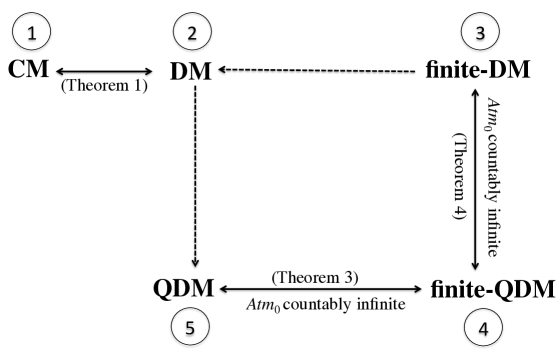
Figure 1: Relations between semantics for the modal language $\mathcal{L}(\mathit{Atm})$. An arrow means that satisfiability relative to the first class of structures implies satisfiability relative to the second class of structures. Full arrows correspond to the results stated in Theorems 1, 3 and 4. Dotted arrows denote relations that follow straightforwardly given the inclusion between classes of structures. The bidirectional arrows connecting node 3 with node 4 and node 4 with node 5 only apply to the infinite-variable case.

3.4 Complexity Results

Let us now move from axiomatics to complexity issues. Our first result is about complexity of checking satisfiability for formulas in $\mathcal{L}(\mathit{Atm})$ relative to the class $\mathbf{CM}$ when $\mathit{Atm}_{0}$ is finite and fixed. It is in line with the satisfiability checking problem of the modal logic S5 which is known to be polynomial in the finite-variable case [18].

Theorem 7.

Let $\mathit{Atm}_{0}$ be finite and fixed. Then, checking satisfiability of formulas in $\mathcal{L}(\mathit{Atm})$ relative to $\mathbf{CM}$ can be done in polynomial time.

As the following theorem indicates, the satisfiability checking problem becomes intractable when dropping the finite-variable assumption.

Theorem 8.

Let $\mathit{Atm}_{0}$ be countably infinite. Then, checking satisfiability of formulas in $\mathcal{L}(\mathit{Atm})$ relative to $\mathbf{CM}$ is NEXPTIME-complete.

Let us consider the following fragment $\mathcal{L}^{\{[\emptyset]\}}(\mathit{Atm})$ of the language $\mathcal{L}(\mathit{Atm})$ where only the universal modality $[\emptyset]$ is allowed:

$\varphi$

$::=$

$p\mid\mathsf{t}({c})\mid\neg\varphi\mid\varphi\wedge\varphi\mid[\emptyset]\varphi.$

Clearly, satisfiability checking for formulas in $\mathcal{L}^{\{[\emptyset]\}}(\mathit{Atm})$ remains polynomial when there are only finitely many primitive propositions. As the following theorem indicates, complexity decreases from NEXPTIME to NP when restricting to the fragment $\mathcal{L}^{\{[\emptyset]\}}(\mathit{Atm})$ under the infinite-variable assumption.

Theorem 9.

Let $\mathit{Atm}_{0}$ be countably infinite. Then, checking satisfiability of formulas in $\mathcal{L}^{\{[\emptyset]\}}(\mathit{Atm})$ relative to $\mathbf{CM}$ is NP-complete.

The complexity results of this section are summarized in Table 1.

	Fixed finite variables	Infinite variables
Fragment $\mathcal{L}^{\{[\emptyset]\}}(\mathit{Atm})$	Polynomial	NP-complete
Full language $\mathcal{L}(\mathit{Atm})$	Polynomial	NEXPTIME-complete

Table 1: Summary of complexity results

4 Counterfactual Conditional

In this section we investigate a simple notion of counterfactual conditional for binary classifiers, inspired from Lewis’ notion [27]. In Section 5, we will elucidate its connection with the notion of explanation.

We start our analysis by defining the following notion of similarity between states in a classifier model relative to a finite set of features $X$.

Definition 10 (Similarity between states).

Let $C=(S,f)$ be a classifier model, $s,s^{\prime}\in S$ and $X\subseteq^{\mathrm{fin}}\mathit{Atm}_{0}$. The similarity between $s$ and $s^{\prime}$ in $S$ relative to the set of features $X$, noted $\mathit{sim}_{C}(s{,}s^{\prime}{,}X)$, is defined as follows:

$$\mathit{sim}_{C}(s{,}s^{\prime}{,}X)=|\{p\in X:(C,s)\models p\text{ iff }(C,s^{\prime})\models p\}|.$$

A dual notion of distance between worlds can defined from the previous notion of similarity:

$$\mathit{dist}_{C}(s{,}s^{\prime}{,}X)=|X|-\mathit{sim}_{C}(s{,}s^{\prime}{,}X).$$

This notion of distance is in accordance with [11] in knowledge revision.

The following definition introduces the notion of counterfactual conditional as an abbreviation. It is a form of relativized conditional, i.e., a conditional with respect to a finite set of features.

Definition 11 (Counterfactual conditional).

We write $\varphi\Rightarrow_{X}\psi$ to mean that “if $\varphi$ was true then $\psi$ would be true, relative to the set of features $X$” and define it as follows:

$$\varphi\Rightarrow_{X}\psi=_{\mathit{def}}\bigwedge_{0\leq k\leq|X|}\big{(}\mathsf{maxSim}(\varphi{,}X{,}k)\rightarrow\bigwedge_{Y\subseteq X:|Y|=k}[Y](\varphi\rightarrow\psi)\big{)},$$

with

$$\mathsf{maxSim}(\varphi{,}X{,}k)=_{\mathit{def}}\bigvee_{Y\subseteq X:|Y|=k}\langle Y\rangle\varphi\wedge\bigwedge_{Y\subseteq X:k<|Y|}[Y]\neg\varphi.$$

As the following proposition highlights, the previous definition of counterfactual conditional is in line with Lewis’ view: the conditional holds if all closest worlds to the actual world in which the antecedent is true satisfy the consequent of the conditional.

Proposition 3.

Let $C=(S,f)$ be a classifier model, $s\in S$ and $X\subseteq^{\mathrm{fin}}\mathit{Atm}_{0}$. Then, $(C,s)\models\varphi\Rightarrow_{X}\psi$ if and only if $\mathit{closest}_{C}(s{,}\varphi{,}X)\subseteq||\psi||_{C}$, where

$$\mathit{closest}_{C}(s{,}\varphi{,}X)=\underset{s^{\prime}\in||\varphi||_{C}}{\arg\max}\ \mathit{sim}_{C}(s{,}s^{\prime}{,}X),$$

and for every $\varphi\in\mathcal{L}(\mathit{Atm})$:

$$||\varphi||_{C}=\{s\in S:(C,s)\models\varphi\}.$$

For notational convenience, we simply write $\varphi\Rightarrow\psi$ instead of $\varphi\Rightarrow_{\mathit{Atm}_{0}}\psi$, when $\mathit{Atm}_{0}$ is finite. Formula $\varphi\Rightarrow\psi$ captures the standard notion of conditional of conditional logic. One can show that $\Rightarrow$ satisfies all semantic conditions of Lewis’ logic $\mathsf{VC}$. However, when $\mathit{Atm}_{0}$ is infinite, $\varphi\Rightarrow\psi$ is not a well-formed formula since it ranges over an infinite set of atoms. In that case $\varphi\Rightarrow_{X}\psi$ has to be always indexed by some finite $X$.

The interesting aspect of the previous notion of counterfactual conditional is that it can be used to represent a binary classifier’s approximate decision for a given instance. Let us suppose the set of decision values $\mathit{Val}$ includes a special symbol $?$ meaning that the classifier has no sufficient information enabling it to classify an instance in a precise way. More compactly, $?$ is interpreted as that the classifier abstains from making a precise decision. In this situation, the classifier can try to make an approximate decision: it considers the closest instances to the actual instance for which it has sufficient information to make a decision and checks whether the decision is uniform among all such instances. In other words, $c$ is the classifier’s approximate classification of (or decision for) the actual instance relative to the set of features $X$, noted $\mathsf{apprDec}(X{,}c)$, if and only if “if a precise decision was made relative to the set of features $X$, then this decision would be $c$”. Formally:

$$\mathsf{apprDec}(X{,}c)=_{\mathit{def}}\big{(}\bigvee_{c^{\prime}\in\mathit{Val}:c^{\prime}\neq?}\mathsf{t}({c^{\prime}})\big{)}\Rightarrow_{X}\mathsf{t}({c}).$$

The following proposition provides two interesting validities.

Proposition 4.

Let $\mathit{Atm}_{0}$ be finite, $c,c^{\prime}\in\mathit{Val}\setminus\{?\}$. Then,

$$\models_{\mathbf{CM}}\mathsf{apprDec}(X,c)\rightarrow\neg\mathsf{apprDec}(X,c^{\prime})\text{ if }c\neq c^{\prime},$$

$$\models_{\mathbf{CM}}\mathsf{t}({c})\rightarrow\mathsf{apprDec}(\mathit{Atm}_{0},c).$$

According to the first validity, a classifier cannot make two different approximate decisions relative to a fixed set of features $X$.

According to the second validity, if the classifier is able to make a precise decision for a given instance, then its approximate decision coincides with it. This second validity works since the actual state/instance is the only closest state/instance to itself. Therefore, it the actual state/instance has a precise classification $c$, all its closest states/instances also have it.

It is worth noting that the following formula is not valid relative to the class $\mathbf{CM}$:

$$\bigvee_{c\in\mathit{Val}\setminus\{?\}}\mathsf{apprDec}(X,c).$$

This means that a classifier may be unable to approximately classify the actual instance. The reason is that there could be different closest states to the actual one with different classifications.

5 Explanations and Biases

In this section, we are going to formalize some existing notions of explanation of classifiers in our logic, and deepen the current study from a (finitely) Boolean setting to a multi-valued output, partial domain and possibly infinite-variable setting. For this purpose it is necessary to introduce the following notations.

Let $\lambda$ denote a conjunction of finitely many literals, where a literal is an atom $p$ or its negation $\neg p$. We write $\lambda\subseteq\lambda^{\prime}$, call $\lambda$ a part (subset) of $\lambda^{\prime}$, if all literals in $\lambda$ also occur in $\lambda^{\prime}$; and $\lambda\subset\lambda^{\prime}$ if $\lambda\subseteq\lambda^{\prime}$ but not $\lambda^{\prime}\subseteq\lambda$. By convention $\top$ is a term of zero conjuncts. In particular, suppose $\lambda$ is $\mathsf{cn}_{X{,}Y}$ for some $X\subseteq Y\subseteq^{\mathrm{fin}}\mathit{Atm}_{0}$, then $\overline{\lambda}$ will denote the conjunction resulting from “flipping” (or “perturbing”) all literals of $\lambda$, i.e., $\mathsf{cn}_{Y\setminus X{,}Y}$.

In the glossary of Boolean classifiers, $\lambda$ is called a term or property (of an instance). The set of terms is noted $\mathit{Term}$. We use $\mathit{Term}(X)$ to denote all terms whose atoms are in $X$. Additionally, to define the notion of bias we distinguish the set of protected features $\text{$\mathsf{PF}$}\subseteq\mathit{Atm}_{0}$, like ‘gender’ and ‘race’, and the set of non-protected features $\text{$\mathsf{NF}$}=\mathit{Atm}_{0}\setminus\text{$\mathsf{PF}$}$.

Notice that in this section the cardinality of $\mathit{Atm}_{0}$ matters. Notions and results in Section 5.1 (without special instruction) apply to both $\mathit{Atm}_{0}$ finite and $\mathit{Atm}_{0}$ countably infinite. On the contrary, in Sections 5.2 and 5.3, we restrict to the case $\mathit{Atm}_{0}$ finite, which is due to the use of formulas $[\mathit{Atm}_{0}\setminus X]\varphi,[\text{$\mathsf{NF}$}]\varphi$ and $[\text{$\mathsf{PF}$}]\varphi$ there. We clarify it here instead of clarifying it below repeatedly.

5.1 Prime Implicant and Abductive Explanation

We are in position to formalize the notion of prime implicant, which plays a fundamental role in the theory of Boolean functions since [39].

Definition 12 (Prime implicant ($\mathsf{PImp}$)).

We write $\text{$\mathsf{PImp}$}(\lambda,c)$ to mean that $\lambda$ is a prime implicant for $c$ and define it as follows:

$$\text{$\mathsf{PImp}$}(\lambda,c)=_{\mathit{def}}[\emptyset]\Big{(}\lambda\to\big{(}\mathsf{t}({c})\wedge\bigwedge_{p\in\mathit{Atm}(\lambda)}\langle\mathit{Atm}(\lambda)\setminus\{p\}\rangle\neg\mathsf{t}({c})\big{)}\Big{)}.$$

It is a proper extension of the definition of prime implicant in the Boolean setting since it is a term $\lambda$ such that 1) it necessarily implies the actual classification (why it is called an implicant); 2) any of its proper subsets fails to necessarily imply the actual classification (why it is called prime). Notice that being a prime implicant is a global property of the classifier, though we formalize it by means of a pointed model. The syntactic abbreviation for prime implicant can be better understood by observing that for a given CM $C=(S,f)$ and $s\in S$, we have:

$$(C,s)\models\text{$\mathsf{PImp}$}(\lambda,c)\text{ iff } (i)\ \forall s^{\prime}\in S,\text{ if }(C,s^{\prime})\models\lambda\text{ then }(C,s^{\prime})\models\mathsf{t}({c});\text{ and }$$

$$(ii)\ \forall\lambda^{\prime}\subset\lambda,\exists s^{\prime}\in S\text{ such that }(C,s^{\prime})\models\lambda^{\prime}\wedge\neg\mathsf{t}({c}).$$

To explain the actual classification of a given input, some XAI researchers consider prime implicants which are actually true. We use the terminology by [24] and call them abductive explanations (AXp).

Definition 13 (Abductive explanation ($\mathsf{AXp}$)).

We write $\textsf{$\mathsf{AXp}$}(\lambda,c)$ to mean that $\lambda$ abductively explains the decision $c$ and define it as follows:

$$\textsf{$\mathsf{AXp}$}(\lambda,c)=_{\mathit{def}}\lambda\wedge\text{$\mathsf{PImp}$}(\lambda,c).$$

AXp is a local explanation, because $\lambda$ is not only a prime implicant for the classification, but also a property of the actual instance to be classified. AXp can be expanded to highlight its connection with the notion of variance/invariance.

Proposition 5.

Let $\lambda\in\mathit{Term}$ and $c\in\mathit{Val}$. Then, we have the following validity:

$$\models_{\mathbf{CM}}\textsf{$\mathsf{AXp}$}(\lambda,c)\leftrightarrow\big{(}\lambda\wedge[\mathit{Atm}(\lambda)]\mathsf{t}({c})\wedge\bigwedge_{p\in\mathit{Atm}(\lambda)}\langle\mathit{Atm}(\lambda)\setminus\{p\}\rangle\neg\mathsf{t}({c})\big{)}.$$

The formula $[\mathit{Atm}(\lambda)]\mathsf{t}({c})$ expresses the idea of invariance under intervention (perturbation): as long as the explanans variables are kept fixed, namely the variables in $\lambda$, any perturbation on the other variables does not change the explanandum, namely classification $c$.

Many names besides AXp are found in literature, e.g., PI-explanation [41] and sufficient reason [12]. Darwiche and Hirth in [12] proved that any decision has a sufficient reason in the Boolean setting. The result is not a surprise, for a Boolean function always has a prime implicant, since by definition the arity of a Boolean function is always finite. However, since we allow functions with infinitely many variables, AXps are not guaranteed to exist in general.

Fact 4.

Let $\mathit{Atm}_{0}$ be countably infinite and $|\mathit{Val}|>1$. Then, there exists some $C=(S,f)$, $s\in S$, such that $\exists c\in\mathit{Val},\forall\lambda\in\mathit{Term},$ $(C,s)\models\neg\textsf{$\mathsf{AXp}$}(\lambda,c)$.

The statement can be proved by exhibiting the same infinite countermodel as in Fact 3 in Section 2.2. However, if a CM is $X$-definite for some $X\subseteq^{\mathrm{fin}}\mathit{Atm}_{0}$, then every state has an AXp, even when the CM is infinite.

Proposition 6.

Let $C=(S,f)\in\mathbf{CM}$ and $X\subseteq^{\mathrm{fin}}\mathit{Atm}_{0}$. If $C$ is $X$-definite then $\forall s\in S,\exists\lambda\in\mathit{Term}\text{ such that }(C,s)\models\textsf{$\mathsf{AXp}$}\big{(}\lambda,f(s)\big{)}$.

Lastly, let us continue with the Alice example.

Example 3.

Recall the state of Alice $s=\{center,employed$}. We have $(C,s)\models\textsf{$\mathsf{AXp}$}(\neg male\wedge\neg owner,0)$, namely that Alice’s being female and not owning a property abductively explains the rejection of her application.

5.2 Contrastive Explanation (CXp)

AXp is a minimal part of the actual instance guaranteeing the current decision. A natural counterpart of AXp is contrastive explanation (CXp, named in [23]).

Definition 14 (Contrastive explanation (CXp)).

We write $\textsf{$\mathsf{CXp}$}(\lambda,c)$ to mean that $\lambda$ contrastively explains the decision $c$ and define it as follows:

$$\textsf{$\mathsf{CXp}$}(\lambda,c)=_{\mathit{def}} \lambda\wedge\langle\mathit{Atm}_{0}\setminus\mathit{Atm}(\lambda)\rangle\neg\mathsf{t}({c})\wedge$$

$$\bigwedge_{p\in Atm(\lambda)}[(\mathit{Atm}_{0}\setminus Atm(\lambda))\cup\{p\}]\mathsf{t}({c}).$$

The definition says nothing but 1) $\lambda$ is part of the actual input instance; 2) if the values of all variables in $\lambda$ are changed while the values of the other variables are kept fixed, then the actual classification may change; 3) the classification will not change, if the variables outside $\lambda$ and at least one variable in $\lambda$ keep their actual values. The latter captures a form of necessity: when the values of the variables outside $\lambda$ are kept fixed, all variables in $\lambda$ should be necessarily perturbed to change the actual classification.

The syntactic abbreviation for contrastive explanation can be better understood by observing that for a given CM $C=(S,f)$ and $s\in S$, we have:

$$(C,s)\models\textsf{$\mathsf{CXp}$}(\lambda,c)\text{ iff } (i)\ (C,s)\models\lambda;$$

$$(ii)\ \exists s^{\prime}\in S\text{ s.t. }s\triangle s^{\prime}=\mathit{Atm}(\lambda)\text{ and }(C,s^{\prime})\models\neg\mathsf{t}({c});\text{ and }$$

$$(iii)\ \forall s^{\prime}\in S,\text{ if }s\triangle s^{\prime}\subset\mathit{Atm}(\lambda)\text{ then }(C,s^{\prime})\models\mathsf{t}({c}).$$

CXp has a counterfactual flavor since it answers to question: would the classification differ from the actual one, if the values of all variables in the explanans were different? So, there seems to be a connection with the notion of counterfactual conditional we introduced in Section 4. Actually in XAI, many researchers consider contrastive explanation and counterfactual explanation either closely related [48] or even interchangeable [42]. The following proposition sheds light on this point.

Proposition 7.

Let $\lambda$ be a term and let $l$ be a literal. Then, we have the following two validities:

$$\models_{\mathbf{CM}} \textsf{$\mathsf{CXp}$}(\lambda,c)\rightarrow\Big{(}\mathsf{t}({c})\wedge\big{(}\overline{\lambda}\Rightarrow\neg\mathsf{t}({c})\big{)}\Big{)},$$

$$\models_{\mathbf{CM}} \mathsf{Comp}(\mathit{Atm}_{0})\to\Big{(}\textsf{$\mathsf{CXp}$}(l,c)\leftrightarrow\Big{(}\mathsf{t}({c})\wedge\big{(}\neg l\Rightarrow\neg\mathsf{t}({c})\big{)}\Big{)}\Big{)}.$$

According to the first validity, in the general case contrastive explanation implies counterfactual explanation. According to the second validity, when the explanans is a literal (a single-conjunct term), contrastive explanation coincides with counterfactual explanation given $\mathit{Atm}_{0}$-completeness. Particularly, literal $l$ contrastively explains the decision $c$ if and only if (i) the actual decision is $c$ and (ii) if literal $l$ were perturbed, the decision would be different from $c$. In other words, in the “atomic” case under the completeness assumption, CXp is the same as counterfactual explanation.

Note that the right-to-left direction of the first validity does not necessarily hold, even after assuming that the classifier is complete with respect to the set of all features $\mathit{Atm}_{0}$. To see this, it is sufficient to suppose that $\mathit{Atm}_{0}=\{p,q\}$ and $\mathit{Dec}=\{0,1\}$ and to consider the CM $(S,f)$ such that $S=2^{\mathit{Atm}_{0}}$ with $f\big{(}\{p,q\}\big{)}=0$ and $f\big{(}\{p\}\big{)}=f\big{(}\{q\}\big{)}=f\big{(}\emptyset\big{)}=1$. It is easy to check that in the model so defined we have

$$\big{(}C,\{p,q\}\big{)}\models\mathsf{t}({0})\wedge\big{(}\overline{p\wedge q}\Rightarrow\neg\mathsf{t}({0})\big{)},$$

but at the same time,

$$\big{(}C,\{p,q\}\big{)}\models\neg\textsf{$\mathsf{CXp}$}(p\wedge q,0).$$

The problem is that the model fails to satisfy the necessity condition of contrastive explanation: it is not necessary to perturb both literals in $p\wedge q$ to change the actual decision from $0$ to $1$, it is sufficient to perturb one of them. We can conclude that CXp is a special kind of counterfactual explanation with the additional requirement of necessity for the explanans.

Example 4.

In Alice’s case, we have $(C,s)\models\textsf{$\mathsf{CXp}$}(\neg male,0)\wedge\textsf{$\mathsf{CXp}$}(\neg owner,0)$. This means that both Alice’s being female and not owning property contrastively explain the rejection. Moreover, we have $(C,s)\models(\neg male\vee\neg owner)\Rightarrow\mathsf{t}({1})$, namely if Alice was a male or an owner (of an immobile property), then her application would have been accepted.

Moreover, since the feature ‘gender’ is hard to change, owing a property is the (relatively) actionable explanation for Alice, if she intends to comply with the classifier’s decision. But surely Alice has another option, i.e., alleging the classifier as biased. As we will see in the next subsection, an application of CXp is to detect decision biases in a classifier.

5.3 Decision Bias

A primary goal of XAI is to detect and avoid biases. Bias is understood as making decision with respect to some protected features, e.g., ‘race’, ‘gender’ and ‘age’.

There is a widely accepted notion of decision bias in the setting of Boolean functions which can be represented in our Example 2 (see [12, 22]). Intuitively, the rejection for Alice is biased if there is another applicant, say Bob, who only differs from Alice on the protected feature ‘gender’, but gets accepted.

Definition 15 (Decision bias).

We write $\text{$\mathsf{Bias}$}(c)$ to mean that the decision $c$ is biased and define it as follows:

$$\text{$\mathsf{Bias}$}(c)=_{\mathit{def}}\mathsf{t}({c})\wedge\langle\text{$\mathsf{NF}$}\rangle\neg\mathsf{t}({c}).$$

The definition says that the decision $c$ is biased at a given state $s$, if (i) $f(s)=c$, and (ii) $\exists s^{\prime}\in S$ such that $s\triangle s^{\prime}\subseteq\text{$\mathsf{PF}$}$ and $f(s^{\prime})\neq c$. The latter, in plain words, requires another instance $s^{\prime}$, which only differs from $s$ on some protected features, but obtains a different classification.

As we stated, CXp can be used to detect decision biases. The following result makes the statement precise.

Proposition 8.

We have the following validity:

$$\models_{\mathbf{CM}} \text{$\mathsf{Bias}$}(c)\leftrightarrow\bigvee_{\mathit{Atm}(\lambda)\subseteq\text{$\mathsf{PF}$}}\textsf{$\mathsf{CXp}$}(\lambda,c).$$

Let us end up the whole section by answering the last question regarding Alice raised at the end of Section 2.1.

Example 5.

Split $\mathit{Atm}_{0}$ in Example 2 into $\text{$\mathsf{PF}$}=\{male,center\}$ and $\text{$\mathsf{NF}$}=\{employed,owner\}$. We then have $(C,s)\models\text{$\mathsf{Bias}$}(0)\wedge\textsf{$\mathsf{CXp}$}(male,0)\wedge\big{(}\neg male\Rightarrow\mathsf{t}({1})\big{)}$. The decision for Alice is biased since ‘gender’ is the protected feature which contrastively explains the rejection, and if Alice was male, her application would have been accepted.

6 Extensions

In this section, we briefly discuss two interesting extensions of our logical framework and analysis of binary classifiers. Their full development is left for future work.

6.1 Dynamic Extension

The first extension we want to discuss consists in adding to the language $\mathcal{L}(\mathit{Atm})$ dynamic operators of the form $[c\!:=\!\varphi]$ with $c\in\mathit{Val}$, where $c\!:=\!\varphi$ is a kind of assignment in the sense of [43, 47] and the formula $[c\!:=\!\varphi]\psi$ has to be read “$\psi$ holds after every decision is set to $c$ in context $\varphi$”. The resulting language, noted $\mathcal{L}^{\mathit{dyn}}(\mathit{Atm})$, is defined by the following grammar:

$\varphi$

$::=$

$p\mid\mathsf{t}({c})\mid\neg\varphi\mid\varphi\wedge\varphi\mid[X]\varphi\mid[c\!:=\!\varphi]\psi,$

where $p$ ranges over $\mathit{Atm}_{0}$, $c$ ranges over $\mathit{Val}$, and $X\subseteq^{\mathrm{fin}}\mathit{Atm}_{0}$. The interpretation of formula $[c\!:=\!\varphi]\psi$ relative to a pointed classifier model $(C,s)$ with $C=(S,f)$ goes as follows:

$$(C,s)\models[c\!:=\!\varphi]\psi \Longleftrightarrow (C^{c:=\varphi},s)\models\psi,$$

where $C^{c:=\varphi}=(S,f^{c:=\varphi})$ is the updated classifier model where, for every $s^{\prime}\in S$:

$$f^{c:=\varphi}(s^{\prime})=\begin{cases}c\text{ if }(C,s^{\prime})\models\varphi,\\ f(s^{\prime})\text{ otherwise}.\end{cases}$$

Intuitively, the operation $c\!:=\!\varphi$ consists in globally classifying all instances satisfying $\varphi$ with value $c$.

Dynamic operators $[c\!:=\!\varphi]$ are useful for modeling a classifier’s revision. Specifically, new knowledge can be injected into the classifier thereby leading to a change in its classification. For example, the classifier could learn that if an object is a furniture, has one or more legs and has a flat top, then it is a table. This is captured by the following assignment:

$$\mathtt{table}\!:=\!\mathit{objIsFurniture}\wedge\mathit{objHasLegs}\wedge\mathit{objHasFlatTop}.$$

An application of dynamic change is to model the training process of a classifier, together with counterfactual conditionals with $``?"$ in Section 4. Suppose at the beginning we have a CM $C=(S,f)$ which is totally ignorant, i.e., $\forall s\in S,f(s)=?$. We then prepare to train the classifier. The training set consists of pairs $(s_{1},x_{1}),(s_{2},x_{2})\dots(s_{n},x_{n})$ where $\forall i\in\{1,\dots,n\}$, $s_{i}\in S,x_{i}\in(\mathit{Val}\setminus\{?\})$ and $\forall j\in\{1,\dots,n\}$, $i\neq j$ implies $s_{i}\neq s_{j}$. We train the classifier by revising it with $[x_{1}:=\widehat{s}_{1}]\dots[x_{n}:=\widehat{s}_{n}]$ one by one. Obviously the order does not matter here. In other words, we re-classify some states. With a bit abuse of notation, let $C^{\mathit{train}}=(S,f^{\mathit{train}})$ denote the model resulting from the series of revisions. We finish training by inducing the final model $C^{\dagger}=(S,f^{\dagger})$ from $C^{\mathit{train}}$, where $\forall s\in S,f^{\dagger}(s)=c$, if $(C^{train},s)\models\mathsf{apprDec}(\mathit{Atm}_{0}{,}c)$, otherwise $f^{\dagger}(s)=f^{\mathit{train}}(s)$. This is an example of modeling a special case of the so-called $k$-nearest neighbour (KNN) classification in machine learning [10], where the distance is measured by cardinality. If a new case/instance has to be classified, we see how the most similar cases to the new case were classified. If all of them ($k$ of them in the case of KNN) were classified using the same category, we put the new case into that category.

The logics $\mathsf{BCL}{-}\mathsf{DC}$ and $\mathsf{WBCL}{-}\mathsf{DC}$ ($\mathsf{BCL}$ and $\mathsf{WBCL}$ with Decision Change) extend the logic $\mathsf{BCL}$ and $\mathsf{WBCL}$ by the dynamic operators $[c\!:=\!\varphi]$. They are defined as follows.

Definition 16 (Logics $\mathsf{BCL}{-}\mathsf{DC}$ and $\mathsf{WBCL}{-}\mathsf{DC}$).

We define $\mathsf{BCL}{-}\mathsf{DC}$ (resp. $\mathsf{WBCL}{-}\mathsf{DC}$) to be the extension of $\mathsf{BCL}$ (resp. $\mathsf{WBCL}$) of Definition 7 (resp. Definition 8) generated by the following reduction axioms for the dynamic operators $[c\!:=\!\varphi]$:

$$[c\!:=\!\varphi]\mathsf{t}({c})\leftrightarrow \big{(}\varphi\vee\mathsf{t}({c})\big{)}$$

$$[c\!:=\!\varphi]\mathsf{t}({c^{\prime}})\leftrightarrow \big{(}\neg\varphi\wedge\mathsf{t}({c^{\prime}})\big{)}\text{ if }c\neq c^{\prime}$$

$$[c\!:=\!\varphi]p\leftrightarrow p$$

$$[c\!:=\!\varphi]\neg\psi\leftrightarrow \neg[c\!:=\!\varphi]\psi$$

$$[c\!:=\!\varphi](\psi_{1}\wedge\psi_{2})\leftrightarrow \big{(}[c\!:=\!\varphi]\psi_{1}\wedge[c\!:=\!\varphi]\psi_{2}\big{)}$$

$$[c\!:=\!\varphi][X]\psi\leftrightarrow [X][c\!:=\!\varphi]\psi$$

and the following rule of inference:

$$\frac{\varphi_{1}\leftrightarrow\varphi_{2}}{\psi\leftrightarrow\psi[\varphi_{1}/\varphi_{2}]}$$ (RE)

It is routine exercise to verify that the equivalences in Definition 16 are valid for the class $\mathbf{CM}$ and that the rule of replacement of equivalents (RE) preserves validity. The completeness of $\mathsf{BCL}{-}\mathsf{DC}$ (resp. $\mathsf{WBCL}{-}\mathsf{DC}$) for this class of models under the finite-variable assumptions (resp. infinite-variable assumption) follows from Corollary 1 (resp. Corollary 2), in view of the fact that the reduction axioms and the rule of replacement of proved equivalents can be used to find, for any $\mathcal{L}^{\mathit{dyn}}$-formula, a provably equivalent $\mathcal{L}$-formula.

Theorem 10.

Let $\mathit{Atm}_{0}$ be finite. Then, the logic $\mathsf{BCL}{-}\mathsf{DC}$ is sound and complete relative to the class $\mathbf{CM}$.

Theorem 11.

Let $\mathit{Atm}_{0}$ be countably infinite. Then, the logic $\mathsf{WBCL}{-}\mathsf{DC}$ is sound and complete relative to the class $\mathbf{CM}$.

The following complexity results are consequences of Theorems 7 and 8 and the fact that via the reduction axioms in Definition 8 we can find a polynomial reduction of satisfiability checking for formulas in $\mathcal{L}^{\mathit{dyn}}$ to satisfiability checking for formulas in $\mathcal{L}$.

Theorem 12.

Let $\mathit{Atm}_{0}$ be finite and fixed. Then, checking satisfiability of formulas in $\mathcal{L}^{\mathit{dyn}}(\mathit{Atm})$ relative to $\mathbf{CM}$ can be done in polynomial time.

Theorem 13.

Let $\mathit{Atm}_{0}$ be countably infinite. Then, checking satisfiability of formulas in $\mathcal{L}^{\mathit{dyn}}(\mathit{Atm})$ relative to $\mathbf{CM}$ is NEXPTIME-complete.

6.2 Epistemic Extension

In the second extension we suppose that a classifier is an agent which has to classify what it perceives. The agent could have uncertainty about the actual instance to be classified since it cannot see all its input features.

In order to represent the agent’s epistemic state and uncertainty, we introduce an epistemic modality of the form $\mathsf{K}$ which is used to represent what the agent knows in the light of what it sees. Similar notions of visibility-based knowledge can be found in [8, 45, 21, 44].

The language for our epistemic extension is noted $\mathcal{L}^{\mathit{epi}}(\mathit{Atm})$ and defined by the following grammar:

$\varphi$

$::=$

$p\mid\mathsf{t}({c})\mid\neg\varphi\mid\varphi\wedge\varphi\mid[X]\varphi\mid\mathsf{K}\varphi,$

where $p$ ranges over $\mathit{Atm}_{0}$, $c$ ranges over $\mathit{Val}$, and $X\subseteq^{\mathrm{fin}}\mathit{Atm}_{0}$.

In order to interpret the new modality $\mathsf{K}$, we have to enrich classifier models with an epistemic component.

Definition 17 (Epistemic classifier model).

An epistemic classifier model (ECM) is a tuple $E=(S,f,\mathit{Obs})$ where $C=(S,f)$ is a classifier model and $\mathit{Obs}\subseteq\mathit{Atm}_{0}$ is the set of atomic propositions that are visible to the agent. The class of ECMs is noted $\mathbf{ECM}$.

Given an ECM $E=(S,f,\mathit{Obs})$, we can define an epistemic indistinguishability relation which represents the agent’s uncertainty about the actual input instance.

Definition 18 (Epistemic indistinguishability relation).

Let $E=(S,f,\mathit{Obs})$ be an ECM. Then, $\sim$ is the binary relation on $S$ such that, for all $s,s^{\prime}\in S$:

$$s\sim s^{\prime}\text{ if and only if }(s\cap\mathit{Obs})=(s^{\prime}\cap\mathit{Obs}).$$

Clearly, the relation $\sim$ so defined is an equivalence relation. According to the previous definition, the agent cannot distinguish between two states $s$ and $s^{\prime}$, noted $s\sim s^{\prime}$, if and only if the truth values of the visible variables are the same at $s$ and $s^{\prime}$.

The interpretation for formulas in $\mathcal{L}^{\mathit{epi}}(\mathit{Atm})$ extends the interpretation for formulas in $\mathcal{L}(\mathit{Atm})$ given in Definition 2 by the following condition for the epistemic operator:

$$(E,s)\models\mathsf{K}\varphi \Longleftrightarrow \forall s^{\prime}\in S:\text{ if }s\sim s^{\prime}\text{ then }(E,s^{\prime})\models\varphi.$$

As the following theorem indicates, the complexity result of Section 3.2 for the finite-variable case generalizes to the epistemic extension.

Theorem 14.

Let $\mathit{Atm}_{0}$ be finite. Then, checking satisfiability of formulas in $\mathcal{L}^{\mathit{epi}}(\mathit{Atm})$ relative to $\mathbf{ECM}$ can be done in polynomial time.

In order to illustrate the intuition behind the epistemic modality $\mathsf{K}$ we go back to the example of the application for a loan to a bank.

Example 6.

Suppose the application is submitted through an online system which has to automatically decide whether it is acceptable or not. In his/her application, an applicant has to specify a value for each feature. Moreover, suppose the system receives an incomplete application: the applicant has only indicated that she is female, owns an apartment and lives in the city center, but she has forgotten to specify whether she has an employment or not. In this case, the value of the employement variable is not “visible” to the system. In formal terms, we extend the CM given in Example 2 by the visibility set $\mathit{Obs}=\{male,center,owner\}$ to obtain a ECM $E=(S,f,\mathit{Obs})$. It is easy to check that the following holds:

$$\big{(}E,\{center,employed,owner\}\big{)}\models\neg\mathsf{K}\ \mathsf{t}({0})\wedge\neg\mathsf{K}\ \mathsf{t}({1}).$$

This means that, on the basis of its partial knowledge of the applicant’s identity, the system does not know what to decide.

However, the system knows that if turns out that the applicant is employed then its application should be accepted:

$$\big{(}E,\{center,employed,owner\}\big{)}\models\mathsf{K}\big{(}employed\rightarrow\mathsf{t}({1})\big{)}.$$

Finally, the classifier knows that if turns out that the applicant is employed, then the fact that she is employed and that she owns a property will abductively explain the decision to accept her application:

$$\big{(}E,\{center,employed,owner\}\big{)}\models\mathsf{K}\big{(}employed\rightarrow\textsf{$\mathsf{AXp}$}(employed\wedge owner,1)\big{)}.$$

7 Conclusion

We have introduced a modal language and a formal semantics that enable us to capture the ceteris paribus nature of binary classifiers. We have formalized in the language a variety of notions which are relevant for understanding a classifier’s behavior including counterfactual conditional, abductive and contrastive explanation, bias. We have provided two extensions that support reasoning about classifier change and a classifier’s uncertainty about the actual instance to be classified. We have also offered axiomatics and complexity results for our logical setting.

We believe that the complexity results presented in the paper are exploitable in practice. We have shown that satisfiability checking in the basic setting and in its dynamic and epistemic extension is polynomial when finitely many variables are assumed. In the infinite-variable setting, it becomes NEXPTIME-complete and NP-complete when restricting to the language in which the only primitive modal operator is the universal modality $[\emptyset]$. In future work, we plan (i) to find a number of satisfiability preserving translations from our modal languages to the modal logic S5 and then from S5 to propositional logic using existing techniques [7], and (ii) to exploit SAT solvers for automated verification and generation of explanations and biases in binary classifiers.

Another direction of future research is the generalization of the epistemic extension given in Section 6.2 to the multi-agent case. The idea is to conceive classifiers as agents and to be able to represent both the agents’ uncertainty about the instance to be classified and their knowledge and uncertainty about other agents’ knowledge and uncertainty (i.e., higher-order knowledge and uncertainty). Similarly, we plan to investigate more in depth classifier dynamics we briefly discussed in Section 6.1. The idea is to see them as learning dynamics. Based on this idea, we plan to study the problem of finding a sequence of update operations guaranteeing that the classifier will be able to make approximate decisions for a given set of instances.

Finally, all classifiers we handle in this paper are essentially “white box”, in the sense that we have perfect knowledge of them, so that we can compute their explanations. However, “black box” classifiers are the most interesting ones to XAI. In [32] we conceived a “black box” classifier as an agent’s uncertainty among many possible “white box” classifiers. We represented it by extending our language with a modal operator ranging over all possible functions which are compatible with the agent’s partial knowledge. All notions of explanation we defined in this paper can be generalized to the “black box” setting. However, there are some important differences between the two settings. For instance, in a “black box” classifier AXp does not always exist, as we showed in [32], which contradicts Proposition 6.

Acknwoledgments

This work is supported by the ANR-3IA Artificial and Natural Intelligence Toulouse Institute (ANITI).

Appendix A Tecnical annex

This technical annex contains a selection of proofs of the results given in the paper.

A.1 Proof of Proposition 2

Proof.

Suppose $C$ is $X$-definite but $(C,s)\models\neg\mathsf{Defin}(X)$, which means that $\exists c\in\mathit{Val}$ s.t. $(C,s)\models\neg=(X,\mathsf{t}({c}))$. W.l.o.g., we assume that $(C,s)\models\neg[\emptyset](\neg\mathsf{t}({c})\to[X]\neg\mathsf{t}({c}))$. That is to say, $\exists s^{\prime}\in S$, s.t. $f(s^{\prime})\neq c$ but $(C,s^{\prime})\models\langle X\rangle\mathsf{t}({c})$. The latter indicates that $\exists s^{\prime\prime}\in S$, s.t. $s^{\prime\prime}\cap X=s^{\prime}\cap X$ but $f(s^{\prime\prime})=c$, which violates $X$-definiteness.

Let $(C,s)\models\mathsf{Defin}(X)$, and assume $f(s)=c$ Then since $(C,s)\models[\emptyset](\mathsf{t}({c})\to[X]\mathsf{t}({c}))$, we have $\forall s^{\prime}\in S$ if $s^{\prime}\cap X=s\cap X$ then $f(s^{\prime})=c=f(s)$, which is what $X$-definiteness says. ∎

A.2 Proof of Theorem 1

Proof.

For the left to right direction, given a CM $C=(S,f)$ and $s_{0}\in S$ s.t. $(C,s_{0})\models\varphi$, we construct a DM $M^{\flat}=(W^{\flat},(\equiv_{X}^{\flat})_{X\subseteq^{\mathrm{fin}}\mathit{Atm}_{0}},V^{\flat})$ as follows

• $W^{\flat}=S$

• $s\equiv_{X}^{\flat}s^{\prime}$ if $s\cap X=s^{\prime}\cap X$

• $V^{\flat}(s)=s\cup\{\mathsf{t}({f(s)})\}$.

It is easy to check that $M^{\flat}$ is indeed a DM and $(M^{\flat},s_{0})\models\varphi$.

For the other direction, given a DM $\big{(}W,(\equiv_{X})_{X\subseteq^{\mathrm{fin}}\mathit{Atm}_{0}},V\big{)}$ and $w_{0}\in W$ s.t. $(M,w_{0})\models\varphi$, we construct a CM $C^{\sharp}=(S^{\sharp},f^{\sharp})$ as follows

• $S^{\sharp}=\{V_{\mathit{Atm}_{0}}(w):w\in W\}$

• $\forall V_{\mathit{Atm}_{0}}(w)\in S^{\sharp},f^{\sharp}(V_{\mathit{Atm}_{0}}(w))=c$, if $V_{\mathit{Dec}}(w)=\{\mathsf{t}({c})\}$.

It is routine to check that $C^{\sharp}$ is a CM, and $(C^{\sharp},V_{\mathit{Atm}_{0}}(w_{0}))\models\varphi$.

∎

A.3 Proof of Theorem 2

Proof.

The proof is conducted by constructing the canonical model.

Definition 19 (Theory).

A set of formulas $\Gamma$ is said to be a $\mathsf{BCL}$-theory if it contains all theorems of $\mathsf{BCL}$ and is closed under MP and Nec_[∅]. It is said to be a consistent $\mathsf{BCL}$-theory if it is a theory and $\bot\notin\Gamma$. It is said to be a maximal consistent $\mathsf{BCL}$-theory (MCT for short), if it is a consistent theory and for all consistent theory $\Gamma^{\prime}$, if $\Gamma\subseteq\Gamma^{\prime}$ then $\Gamma=\Gamma^{\prime}$.

Lemma 1 (Lindenbaum-type).

Let $\Delta$ be a consistent $\mathsf{BCL}$-theory and $\varphi\notin\Delta$ Then, there is a maximal consistent $\mathsf{BCL}$-theory $\Gamma$ s.t. $\Delta\subseteq\Gamma$ and $\varphi\notin\Gamma$.

The proof is standard and omitted (see, e.g. [5, p. 197] ).

Definition 20 (Canonical model).

The canonical decision model $\text{$\mathfrak{M}$}=(W^{c},(\equiv_{X}^{c})_{X\subseteq^{\mathrm{fin}}\mathit{Atm}_{0}},V^{c})$ is defined as follows

• $W^{c}=\{\Gamma:\Gamma\text{ is a maximal consistent }\mathsf{BCL}\text{ theory.}\}$

• $\Gamma\equiv^{c}_{X}\Delta\iff\{[X]\varphi:[X]\varphi\in\Gamma\}=\{[X]\varphi:[X]\varphi\in\Delta\}$

• $V^{c}(\Gamma)=\{p:p\in\Gamma\}$

We omit the superscript ^c whenever there is no misunderstanding.

Lemma 2.

Let $\Gamma$ be an MCT. Then $[X]\varphi\to\varphi\in\Gamma$.

Proof.

Suppose $[X]\varphi\to\varphi\notin\Gamma$, then by the maximality of $\Gamma$ and $\mathbf{Red}_{[\emptyset]}$, we have $\bigwedge_{Y\subseteq X}\big{(}\mathsf{cn}_{Y{,}X}\to[\emptyset](\mathsf{cn}_{Y{,}X}\to\varphi)\big{)}\wedge\neg\varphi\in\Gamma$. Since $\Gamma$ is maximally consistent, there is exactly one $Z\subseteq X$ s.t. $\mathsf{cn}_{Z{,}X}\in\Gamma$. By $\mathbf{MP}$ we have $[\emptyset](\mathsf{cn}_{Z{,}X}\to\varphi)\in\Gamma$, and by $\mathbf{K}_{[\emptyset]}$ and $\mathbf{MP}$ we have $\varphi\in\Gamma$. But than $\Gamma$ is inconsistent, since $\varphi\wedge\neg\varphi\in\Gamma$. Hence the supposition fails, which means $[X]\varphi\to\varphi\in\Gamma$. ∎

Lemma 3.

The canonical model $\mathfrak{M}$ is indeed a decision model.

Proof.

Check the conditions one by one. For C1, we need show $\Gamma\equiv^{c}_{X}\Delta$, if $\forall p,p\in V(\Gamma)\cap X$ implies $p\in V(\Delta)$. Suppose not, then w.l.o.g. we have some $q\in V(\Gamma)\cap X,q\notin V(\Delta)$, by maximality of $\Delta$ namely $\neg q\in\Delta$. However, we have $[q]q\in\Gamma$, for $q\to[q]q$ is a theorem, and by definition of $\equiv^{c}_{X},[q]q\in\Delta$, hence $q\in\Delta$, since $[q]q\to q\in\Delta$. But now we have a contradiction. C2-4 hold obviously due to axioms $\mathbf{AtLeast},\mathbf{AtMost}$, $\mathbf{Def}$ and $\mathbf{Funct}$ respectively. ∎

Lemma 4 (Existence).

Let $\text{$\mathfrak{M}$}=(W^{c},(\equiv_{X}^{c})_{X\subseteq^{\mathrm{fin}}\mathit{Atm}_{0}},V^{c})$ be the canonical model, $\Gamma$ be an MCT. Then, if $\langle\emptyset\rangle\varphi\in\Gamma$ then $\exists\Gamma^{\prime}\in W^{c}$ s.t. $\Gamma\equiv_{\emptyset}^{c}\Gamma^{\prime}$ and $\varphi\in\Gamma^{\prime}$.

The proof is following the same line in e.g. [5, p. 198-199] and omitted.

Lemma 5 (Truth).

Let $\mathfrak{M}$ be the canonical model, $\Gamma$ be an MCT, $\varphi\in\mathcal{L}(\mathit{Atm}_{0})$. Then $\text{$\mathfrak{M}$},\Gamma\models\varphi\iff\varphi\in\Gamma$.

Proof.

By induction on $\varphi$. We only show the interesting case when $\varphi$ takes the form $[X]\psi$.

For $\Longleftarrow$ direction, if $[X]\psi\in\Gamma$, since for any $\Delta\equiv_{X}\Gamma$, $[X]\psi\in\Delta$, then thanks to $[X]\psi\to\psi\in\Delta$ we have $\psi\in\Delta$. By induction hypothesis this means $\Delta\models\psi$, therefore $\Gamma\models[X]\psi$.

For $\Longrightarrow$ direction, suppose not, namely $[X]\psi\notin\Gamma$. Then consider a theory $\Gamma^{\prime}=\{\neg\psi\}\cup\{[X]\chi:[X]\chi\in\Gamma\}$. It is consistent since $\psi\notin\Gamma$. Then take any $\Delta\in W$ s.t. $\Gamma^{\prime}\subseteq\Delta$. We have $\Delta\equiv_{X}\Gamma$, but $\Delta\nvDash\psi$ by induction hypothesis. However, this contradicts $\Gamma\models[X]\psi$. ∎

Now the completeness of $\mathbf{DM}$ w.r.t. $\mathsf{BCL}$ is a corollary of Lemma 3 and 5.

∎

A.4 Proof of Theorem 3

Proof.

Let $\big{(}W,(\equiv_{X})_{X\subseteq^{\mathrm{fin}}\mathit{Atm}_{0}},V\big{)}$ be a QDM and $w_{0}\in W$ s.t. $(M,w_{0})\models\varphi$. Let $\mathit{sf}(\varphi)$ be the set of all subformulas of $\varphi$ and let $\mathit{sf}^{+}(\varphi)=\mathit{sf}(\varphi)\cup\mathit{Dec}$. Moreover, $\forall v,u\in W$, we define $v\simeq u\iff$ $\forall\psi\in\mathit{sf}^{+}(\varphi)$, $(M,v)\models\psi$ iff $(M,u)\models\psi$. Finally, we define $[v]=\{u\in W:v\simeq u\}$.

Now we construct a filtration through $\mathit{sf}^{+}(\varphi)$, $M^{\prime}=(W^{\prime},(\equiv_{X}^{\prime})_{X\subseteq^{\mathrm{fin}}\mathit{Atm}_{0}},V^{\prime})$ as follows

• $W^{\prime}=\{[v]:v\in W\}$

• $\forall X\subseteq^{\mathrm{fin}}\mathit{Atm}_{0}$, $[v]\equiv_{X}^{\prime}[u]$, iff $V_{X}^{\prime}([v])=V_{X}^{\prime}([u])$

• $V^{\prime}([v])=V_{\mathit{sf}^{+}(\varphi)\cap\mathit{Atm}_{0}}(v)$

$M^{\prime}$ is indeed a filtration. We need show that it satisfies the two conditions.

1) $v\equiv_{X}u\iff V_{X}(v)=V_{X}(u)\Longrightarrow V_{X}^{\prime}([v])=V_{X}^{\prime}([u])$ $\iff[v]\equiv_{X}^{\prime}[u]$. Suppose $v\equiv_{X}u$. By construction of $V^{\prime}$, $\forall p\in X\cap\mathit{sf}^{+}(\varphi),p\in V_{X}^{\prime}([v])p\in V(v)\iff p\in V(u)\iff p\in V_{X}^{\prime}([u])$, and $\forall p\in X\setminus\mathit{sf}^{+}(\varphi),p\notin V_{X}^{\prime}([v])$ and $p\notin V_{X}^{\prime}([u])$. As a result, $V_{X}^{\prime}([v])=V_{X}^{\prime}([u])$ which means $[v]\equiv_{X}^{\prime}[u]$.

2) If $[v]\equiv_{X}^{\prime}[u]$, then $\forall[X]\psi\in\mathit{sf}^{+}(\varphi)$: if $(M,v)\models[X]\psi$ then $(M,u)\models\psi$. The crucial point is that $\forall v,v^{\prime}\in[v],\forall u,u^{\prime}\in[u]$, $\forall[X]\psi\in\mathit{sf}^{+}(\varphi)$, if $[v]\equiv_{X}^{\prime}[u]$, then $v\equiv_{X}v^{\prime}\equiv_{X}u\equiv_{X}u^{\prime}$ by the definitions of $V^{\prime}$ and $\simeq$. Hence by satisfaction relation of $M$ we have if $(M,v)\models[X]\psi$ then $(M,u)\models\psi$.

Moreover, $M^{\prime}$ is a finite-QDM. For $\mathbf{C1}$ it is given as the definition of $V^{\prime}$. $\mathbf{C2}$ and $\mathbf{C3}$ hold because of $\mathit{sf}^{+}(\varphi)=\mathit{sf}(\varphi)\cup\mathit{Dec}$.

Finally, we need prove $(M,w_{0})\models\varphi$ iff $(M^{\prime},[w_{0}])\models\varphi$. We only show when $\varphi$ takes the form $[X]\psi$. Given $(M,w_{0})\models[X]\psi$, i.e. $\forall v\in W$, if $w_{0}\equiv_{X}v$ then $(M,v)\models\psi$. By definitions of $\equiv_{X}^{\prime}$ and $\mathbf{C1}$ we have $V_{X}^{\prime}([w_{0}])=V_{X}^{\prime}([v])$, by induction hypothesis $(M^{\prime},[v])\models\psi$, which means $(M^{\prime},[w_{0}])\models[X]\psi$. If $(M^{\prime},[w_{0}])\models[X]\psi$, i.e. $\forall[v]\in W^{\prime}$, if $[v]\equiv_{X}^{\prime}[w_{0}]$ then $(M^{\prime},[v])\models\psi$. Then by definitions of $V^{\prime}$ and $\simeq$ we have $w_{0}\equiv_{X}v$, by induction hypothesis $(M,v)\models\psi$. ∎

A.5 Proof of Theorem 4

Proof.

The right to left direction is obvious since any finite-DM is a finite-QDM. For the other direction, suppose there is a finite-QDM $\big{(}W,(\equiv_{X})_{X\subseteq^{\mathrm{fin}}\mathit{Atm}_{0}},V\big{)}$ and $w\in W$ s.t. $(M,w)\models\varphi$. Since $\mathit{Atm}_{0}$ is infinite, we can construct an injection $\iota:W\longrightarrow\mathit{Atm}_{0}\setminus\mathit{Atm}(\varphi)$. Then, we construct a finite-DM $M^{\prime}=(W^{\prime},(\equiv_{X}^{\prime})_{X\subseteq^{\mathrm{fin}}\mathit{Atm}_{0}},V^{\prime})$ as follows

• $W^{\prime}=W$

• $w\equiv_{X}^{\prime}v$ iff $V^{\prime}_{X}(w)=V^{\prime}_{X}(v)$

• $V^{\prime}(w)=(V(w)\cup\{\iota(w)\})\setminus\{p:\exists v\in W,v\neq w\ \&\ \iota(v)=p\}$.

It is easy to check that $M^{\prime}$ is indeed a finite-DM. By induction we show that $(M^{\prime},w)\models\varphi$. When $\varphi$ is some $p$, we have $V(w)=V^{\prime}(w)$ since the injection $\iota$ has nothing to do with $\varphi$. The case of $\mathsf{t}({c})$ is the same. The Boolean cases are straightforward. Finally when $\varphi$ takes form $[X]\psi$. Again since $\iota$ does not change valuation in $\varphi$, we have $\forall v\in W,V_{X}(v)=V^{\prime}_{X}(v)$. Hence we have $(M,w)\models[X]\psi\iff\forall v\in W,$ if $V_{X}(w)=V_{X}(v)$ then $(M,v)\models\psi$ $\iff\forall v\in W,$ if $V^{\prime}_{X}(w)=V^{\prime}_{X}(v)$ then $(M^{\prime},v)\models\psi\iff(M^{\prime},w)\models[X]\psi$. ∎

A.6 Proof of Theorem 7

Proof.

Suppose $\mathit{Atm}_{0}$ is finite and fixed. In order to determine whether a formula $\varphi$ is satisfiable for the class $\mathbf{CM}$, we are going to verify whether $\varphi$ is satisfied in each CM, by doing this sequentially one CM after the other. The corresponding algorithm runs in polynomial time in the size of $\varphi$ since: (i) there is a finite, constant number of CMs and (ii) model checking for the language $\mathcal{L}(\mathit{Atm})$ relative to a pointed CM is polynomial. This means that, when $\mathit{Atm}_{0}$ is finite and fixed, satisfiability checking has the same complexity as model checking. Regarding (i), the finite, constant number of CMs in the class $\mathbf{CM}$ is $\sum_{S\subseteq 2^{\mathit{Atm}_{0}}}|\mathit{Val}|^{|S|}$. Indeed, for every $S\subseteq 2^{\mathit{Atm}_{0}}$, we consider the number of functions from $S$ to $\mathit{Val}$. Regarding (ii), it is easy to build a model checking algorithm running in polynomial time. It is sufficient to adapt the well-known “labelling” model checking algorithm for the basic multimodal logics and CTL [9]. The general idea of the algorithm is to label the states of a finite model step-by-step with sub-formulas of the formula $\varphi$ to be checked, starting from the smallest ones, the atomic propositions appearing in $\varphi$. At each step, a formula should be added as a label to just those states of the model at which it is true.

∎

A.7 Proof of Theorem 8

Proof.

As for NEXPTIME-hardness, in [17] the following ceteris paribus modal language, noted $\mathcal{L}_{\mathsf{CP}}(\mathit{Prop})$, is considered with $\mathit{Prop}$ a countable set of atomic propositions:

$\varphi$

$::=$

$p\mid\neg\varphi\mid\varphi\wedge\varphi\mid[X]\varphi,$

where $p$ ranges over $\mathit{Prop}$ and $X$ is a finite set of atomic propositions from $\mathit{Prop}$. Formulas for this language are interpreted relative to a simple model $S\subseteq 2^{\mathit{Atm}_{0}}$ and a state $s\in S$ in the expected way as follows (we omit boolean cases since they are interpreted in the usual way): $(S,s)\models p\text{ iff }p\in s$; $(S,s)\models[X]\varphi\text{ iff }\forall s^{\prime}\in S:\text{ if }s\cap X=s^{\prime}\cap X\text{ then }(S,s^{\prime})\models\varphi$. It is proved that, when $\mathit{Prop}$ is countably infinite, satisfiability checking for formulas in $\mathcal{L}_{\mathsf{CP}}(\mathit{Prop})$ relative to the class $\mathbf{SM}$ of simple models is NEXPTIME-hard [17, Lemma 2 and Corollary 2]. It follows that satisfiability checking for formulas in our language $\mathcal{L}(\mathit{Atm})$ with $\mathit{Atm}_{0}$ countably infinite is NEXPTIME-hard too.

As for membership, let $tr$ be the following translation from the language $\mathcal{L}(\mathit{Atm})$ to the language $\mathcal{L}_{\mathsf{CP}}\big{(}\mathit{Atm}_{0}\cup\{p_{\mathsf{t}({c})}:c\in\mathit{Val}\}\big{)}$:

$$tr(p)=p,$$

$$tr(\mathsf{t}({c}))=p_{\mathsf{t}({c})},$$

$$tr(\neg\varphi)=\neg tr(\varphi),$$

$$tr(\varphi\wedge\psi)=tr(\varphi)\wedge tr(\psi),$$

$$tr([X]\varphi)=[X]tr(\varphi).$$

By induction on the structure of $\varphi$, it is routine to verify that $\varphi\in\mathcal{L}(\mathit{Atm})$ is satisfiable for the class $\mathbf{QDM}$ of Definition 9 if and only if $[\emptyset]\big{(}\varphi_{1}\wedge\varphi_{2}\big{)}\wedge tr(\varphi)$ is satisfiable for the class $\mathbf{SM}$ of simple models, with

$$\varphi_{1}=_{\mathit{def}} \bigvee_{c\in\mathit{Val}}p_{\mathsf{t}({c})},$$

$$\varphi_{2}=_{\mathit{def}} \bigwedge_{c,c^{\prime}\in\mathit{Val}:c\neq c^{\prime}}\big{(}p_{\mathsf{t}({c})}\rightarrow\neg p_{\mathsf{t}({c^{\prime}})}\big{)}.$$

Hence, by Theorem 5 we have that, when $\mathit{Atm}_{0}$ is countably infinite, $\varphi\in\mathcal{L}(\mathit{Atm})$ is satisfiable for the class $\mathbf{CM}$ of classifier models if and only if $[\emptyset]\big{(}\varphi_{1}\wedge\varphi_{2}\big{)}\wedge tr(\varphi)$ is satisfiable for the class $\mathbf{SM}$ of simple models. Since the translation $tr$ is linear and satisfiability checking for formulas in $\mathcal{L}_{\mathsf{CP}}\big{(}\mathit{Atm}_{0}\cup\{p_{\mathsf{t}({c})}:c\in\mathit{Val}\}\big{)}$ relative to the class $\mathbf{SM}$ is in NEXPTIME in the infinite-variable case [17, Lemma 2 and Corollary 1], checking satisfiability of formulas in $\mathcal{L}(\mathit{Atm})$ relative to the class $\mathbf{CM}$ is in NEXPTIME too, with $\mathit{Atm}_{0}$ countably infinite.

∎

A.8 Proof of Theorem 9

Proof.

NP-hardness follows from the NP-harndess of propositional logic.

In order to prove NP-membership, we can use the translation given in the proof of Theorem 8 to give a polynomial reduction of satisfiability checking of formulas in $\mathcal{L}^{\{[\emptyset]\}}(\mathit{Atm})$ relative to $\mathbf{CM}$ to satisfiability checking in the modal logic S5. The latter problem is known to be in NP in the infinite-variable case [26]. ∎

A.9 Proof of Proposition 3

Proof.

For the right direction, we have $\mathit{closest}_{C}(s{,}\varphi{,}X)\subseteq||\psi||_{C}$ from the antecedent. Suppose towards a contradiction that the consequent does not hold. Then, $\exists k\in\{0,\dots,|X|\},Y_{1},Y_{2}\subseteq X$ with $|Y_{1}|=|Y_{2}|=k$, s.t. $(C,s)\models\langle Y_{1}\rangle\varphi\wedge\bigwedge_{Y\subseteq X:k<|Y|}[Y]\neg\varphi\wedge\langle Y_{2}\rangle(\varphi\wedge\neg\psi)$. The last conjunct means that $\exists s^{\prime}\in S,s^{\prime}\cap X=s\cap X=Y_{2}$ and $(C,s^{\prime})\models\varphi\wedge\neg\psi$. But the conjuncts together guarantee that $s^{\prime}\in\mathit{closest}_{C}(s{,}\varphi{,}X)$, because $\mathit{sim}_{C}(s{,}s^{\prime}{,}X)=k$, and it is an argmax by definition of $\mathit{closest}_{C}(s{,}\varphi{,}X)$. It is the desired contradiction, since $s^{\prime}\notin||\psi||_{C}$.

For the other direction, we need show $\mathit{closest}_{C}(s{,}\varphi{,}X)\subseteq||\psi||_{C}$, given the antecedent. Suppose the opposite towards a contradiction. Then by definition, $\exists s^{*}\in\mathit{closest}_{C}(s{,}\varphi{,}X),s^{\prime}\notin||\psi||_{C}$. Let $s\cap X=s^{*}\cap X=Y^{*}$, and $\mathit{sim}_{C}(s{,}s^{\prime}{,}X)=k^{*}$. Then we have $(C,s)\models\mathsf{maxSim}(\varphi{,}X{,}k^{*})\wedge\langle Y^{*}\rangle(\varphi\wedge\neg\psi)$, which contradicts the antecedent. To see that, notice the second conjunct is because of $(C,s^{*})\models\varphi\wedge\neg\psi$, and the first conjunct because of $\mathit{sim}_{C}(s{,}s^{*}{,}X)=k^{*}$ and $s^{*}\in\mathit{closest}_{C}(s{,}\varphi{,}X)$. ∎

A.10 Proof of Proposition 4

Proof.

The first validity is obvious, since if $\mathit{closest}_{C}(s{,}\varphi{,}X)\subseteq||\mathsf{t}({c})||_{C}$ then $\mathit{closest}_{C}(s{,}\varphi{,}X)\nsubseteq||\mathsf{t}({c^{\prime}})||_{C}$ given $c^{\prime}\neq c$. For the second validity, notice that $\{s\}=\mathit{closest}_{C}(s{,}\varphi{,}{\mathit{Atm}_{0}})$, if $(C,s)\models\varphi$. Hence if $(C,s)\models\mathsf{t}({c})$, then we have $\mathit{closest}_{C}(s{,}\bigvee_{c^{\prime}\in\mathit{Val}:c^{\prime}\neq?}{,}\mathit{Atm}_{0})=\{s\}\subseteq||\mathsf{t}({c})||_{C}$. ∎

A.11 Proof of Proposition 5

Proof.

Let $(C,s)$ be a pointed CM and $(C,s)\models\textsf{$\mathsf{AXp}$}(\lambda,c)$, which directly gives us $(C,s)\models\lambda$. Now since $\lambda$ is an implicant of $c$, $(C,s)\models[\mathit{Atm}(\lambda)]\mathsf{t}({c})$, for otherwise $\exists s^{\prime}$, s.t. $(C,s^{\prime})\models\lambda\wedge\neg\mathsf{t}({c})$; and since $\lambda$ is prime, we have $(C,s)\models\bigwedge_{p\in\mathit{Atm}(\lambda)}\langle\mathit{Atm}(\lambda)\setminus\{p\}\rangle\neg\mathsf{t}({c}))$, otherwise $\exists\lambda^{\prime}$, s.t. $\lambda^{\prime}\subset\lambda$ and $\lambda^{\prime}$ is also an implicant of $c$. The other direction is proven in the same way and omitted. ∎

A.12 Proof of Proposition 6

Proof.

Suppose towards a contradiction that $C$ is finitely-definite, but $\exists c\in\mathit{Val}$, s.t. $\forall\lambda\in\mathit{Term}$, if $(C,s)\models\lambda$ then $(C,s)\models\neg\text{$\mathsf{PImp}$}(\lambda,c)$. That is to say, $\exists s_{1}\in S$ s.t. $(M,s_{1})\models\lambda$ but either $f(s_{1})\neq c$ or $\exists s_{2}\in S$ s.t. $\exists p\in\mathit{Atm}(\lambda)$, $s_{1}\cap(\mathit{Atm}(\lambda\setminus\{p\})=s_{2}\cap(\mathit{Atm}(\lambda\setminus\{p\})$ but $f(s_{2})\neq c$. Hence $C$ is neither $\mathit{Atm}(\lambda)$-definite nor $(\mathit{Atm}(\lambda\setminus\{p\})$-definite. Either case $C$ is not finitely-definite, since $\lambda$ is arbitrarily selected from $\mathit{Term}$. ∎

A.13 Proof of Proposition 7

Proof.

For the first validity, let $C=(S,f)\in\mathbf{CM}$ and $s\in S$ and suppose $(C,s)\models\textsf{$\mathsf{CXp}$}(\lambda,c)$. By definition of $\textsf{$\mathsf{CXp}$}(\lambda,c)$ we have $(C,s)\models\mathsf{t}({c})$. We need to show $(C,s)\models\overline{\lambda}\Rightarrow\neg\mathsf{t}({c})$. By the antecedent, $\exists s^{\prime}\in S$, s.t. $s\triangle s^{\prime}=\mathit{Atm}(\lambda)$ and $f(s^{\prime})\neq c$. It is not hard to show that $\mathit{closest}_{C}(s{,}\overline{\lambda}{,}\mathit{Atm})=\{s^{\prime}\}$. Therefore $(C,s)\models\overline{\lambda}\Rightarrow\neg\mathsf{t}({c})$, since $\mathit{closest}_{C}(s{,}\overline{\lambda}{,}\mathit{Atm}_{0})\subseteq||\neg\mathsf{t}({c})||_{C}$. For the second validity, the right direction of the iff is a special case of the first validity. To show the left direction, from $\mathit{Atm}_{0}$-completeness and the counterfactual conditional we have $\exists s^{\prime}\in S$, s.t. $s^{\prime}\triangle s=\mathit{Atm}(l)$ and $\{s^{\prime}\}=\mathit{closest}_{C}(s{,}l{,}\mathit{Atm}_{0})$. Hence $(C,s)\models l\wedge\langle\mathit{Atm}_{0}\setminus\mathit{Atm}(l)\rangle\neg\mathsf{t}({c})\wedge[\mathit{Atm}_{0}]\mathsf{t}({c})$, which is by definition $(C,s)\models\textsf{$\mathsf{CXp}$}(l,c)$. ∎

A.14 Proof of Proposition 8

Proof.

We show that for any $C=(S,f)\in\mathbf{CM}$, both directions are satisfied in $(C,s)$ for some $s\in S$. The right to left direction is obvious, since from the antecedent we know there is a property $\lambda^{\prime}$ s.t. $\exists s^{\prime}\in S,s\triangle s^{\prime}=\mathit{Atm}(\lambda^{\prime})\subseteq\text{$\mathsf{PF}$}$ and $(C,s^{\prime})\models\neg\mathsf{t}({c})$, which means $(C,s)\models\text{$\mathsf{Bias}$}(c)$. The other direction is proven by contraposition. Suppose for any $\lambda$ s.t. $\mathit{Atm}(\lambda)\subseteq\text{$\mathsf{PF}$}$, $(C,s)\models\neg\textsf{$\mathsf{CXp}$}(\lambda,c)$, then it means $\forall s^{\prime}\in S$, if $s\triangle s^{\prime}=\mathit{Atm}(\lambda)$, then $f(s^{\prime})=c$, which means $(C,s)\models\neg\text{$\mathsf{Bias}$}(c)$. ∎

A.15 Proof of Theorem 14

Proof.

Suppose $|\mathit{Atm}_{0}|$ is finite. As in the proof of Theorem 7, we can show that the size of the model class $\mathbf{ECM}$ is bounded by some fixed integer. Thus, in order to determine whether a formula $\varphi$ $\mathcal{L}^{\mathit{epi}}(\mathit{Atm})$ is satisfiable for this class, it is sufficient to repeat model checking a number of times which is bounded by some integer. Model checking for the language $\mathcal{L}^{\mathit{epi}}(\mathit{Atm})$ with respect to a pointed ECM is polynomial. ∎

References

- [1] Leila Amgoud and Jonathan Ben-Naim. Axiomatic foundations of explainability. In 31st International Joint Conference on Artificial Intelligence (IJCAI 2022), 2022.
- [2] Gilles Audemard, Steve Bellart, Louenas Bounia, Frédéric Koriche, Jean-Marie Lagniez, and Pierre Marquis. On the computational intelligibility of boolean classifiers. In Proceedings of the International Conference on Principles of Knowledge Representation and Reasoning, volume 18, pages 74–86, 2021.
- [3] Alexandru Baltag and Johan van Benthem. A simple logic of functional dependence. Journal of Philosophical Logic, 50(5):939–1005, 2021.
- [4] Or Biran and Courtenay Cotton. Explanation and justification in machine learning: A survey. In IJCAI-17 workshop on explainable AI (XAI), volume 8(1), pages 8–13, 2017.
- [5] Patrick Blackburn, Maarten de Rijke, and Yde Venema. Modal Logic. Cambridge University Press, Cambridge, Massachusetts, 2001.
- [6] Alexander Borgida. Language features for flexible handling of exceptions in information systems. ACM Transactions on Database Systems (TODS), 10(4):565–603, 1985.
- [7] Thomas Caridroit, Jean-Marie Lagniez, Daniel Le Berre, Tiago de Lima, and Valentin Montmirail. A SAT-based approach for solving the modal logic s5-satisfiability problem. In Proceedings of the Thirty-First AAAI Conference on Artificial Intelligence (AAAI-17), pages 3864–3870. AAAI Press, 2017.
- [8] Tristan Charrier, Andreas Herzig, Emiliano Lorini, Faustine Maffre, and François Schwarzentruber. Building epistemic logic from observations and public announcements. In Proceedings of the Fifteenth International Conference on Principles of Knowledge Representation and Reasoning (KR 2016), pages 268–277. AAAI Press, 2016.
- [9] Edmund M. Clarke and Bernd-Holger Schlingloff. Model checking. In Alan J. A. Robinson and Andrei Voronkov, editors, Handbook of automated reasoning, pages 1635–1790. Elsevier, 2001.
- [10] Padraig Cunningham and Sarah Jane Delany. K-nearest neighbour classifiers - a tutorial. ACM Computing Surveys, 54(6):1–25, 2022.
- [11] Mukesh Dalal. Investigations into a theory of knowledge base revision: preliminary report. In Proceedings of the Seventh National Conference on Artificial Intelligence, volume 2, pages 475–479. Citeseer, 1988.
- [12] Adnan Darwiche and Auguste Hirth. On the reasons behind decisions. In 24th European Conference on Artificial Intelligence (ECAI 2020), volume 325 of Frontiers in Artificial Intelligence and Applications, pages 712–720. IOS Press, 2020.
- [13] Amit Dhurandhar, Pin-Yu Chen, Ronny Luss, Chun-Chen Tu, Paishun Ting, Karthikeyan Shanmugam, and Payel Das. Explanations based on the missing: Towards contrastive explanations with pertinent negatives. In Advances in Neural Information Processing Systems, pages 592–603, 2018.
- [14] Ronald Fagin, Yoram Moses, Joseph Y Halpern, and Moshe Y Vardi. Reasoning about Knowledge. MIT Press, 1995.
- [15] Patrick Girard and Marcus Anthony Triplett. Ceteris paribus logic in counterfactual reasoning. In Proceedings of the Fifteenth Conference on Theoretical Aspects of Rationality and Knowledge (TARK 2015), pages 176–193, 2016.
- [16] Nelson Goodman. Fact, fiction, and forecast. Harvard University Press, 1955.
- [17] Davide Grossi, Emiliano Lorini, and François Schwarzentruber. The ceteris paribus structure of logics of game forms. Journal of Artificial Intelligence Research, 53:91–126, 2015.
- [18] Joseph Y. Halpern. The effect of bounding the number of primitive propositions and the depth of nesting on the complexity of modal logic. Artificial Intelligence, 75(2):361–372, 1995.
- [19] Joseph Y Halpern. Actual causality. MiT Press, 2016.
- [20] Carl G. Hempel and Paul Oppenheim. Studies in the logic of explanation. Philosophy of science, 15(2):135–175, 1948.
- [21] Andreas Herzig, Emiliano Lorini, and Faustine Maffre. A poor man’s epistemic logic based on propositional assignment and higher-order observation. In Proceedings of the 5th International Workshop on Logic, Rationality, and Interaction, Lecture Notes in Computer Science, pages 156–168. Springer, 2015.
- [22] Alexey Ignatiev, Martin C. Cooper, Mohamed Siala, Emmanuel Hebrard, and Joao Marques-Silva. Towards formal fairness in machine learning. In International Conference on Principles and Practice of Constraint Programming, pages 846–867. Springer, 2020.
- [23] Alexey Ignatiev, Nina Narodytska, Nicholas Asher, and Joao Marques-Silva. From contrastive to abductive explanations and back again. In International Conference of the Italian Association for Artificial Intelligence, pages 335–355. Springer, 2020.
- [24] Alexey Ignatiev, Nina Narodytska, and Joao Marques-Silva. Abduction-based explanations for machine learning models. In Proceedings of the Thirty-third AAAI Conference on Artificial Intelligence (AAAI-19), volume 33, pages 1511–1519, 2019.
- [25] Boris Kment. Counterfactuals and explanation. Mind, 115(458):261–310, 2006.
- [26] Richard E. Ladner. The computational complexity of provability in systems of modal propositional logic. SIAM journal on computing, 6(3):467–480, 1977.
- [27] David K. Lewis. Counterfactuals. Harvard University Press, 1973.
- [28] David K. Lewis. Counterfactual dependence and time’s arrow. Noûs, pages 455–476, 1979.
- [29] David K. Lewis. Causal explanation. In Philosophical Papers, volume 2, pages 214–240. Oxford University Press, 1986.
- [30] David K. Lewis. Causation. Journal of Philosophy, 70(17):556–567, 1995.
- [31] Xinghan Liu and Emiliano Lorini. A logic for binary classifiers and their explanation. In P. Baroni, C. Benzmüller, and Y. N. Wáng, editors, Logic and Argumentation - 4th International Conference, CLAR 2021, Hangzhou, China, 2021, Proceedings, Lecture Notes in Computer Science, pages 302–321. Springer, 2021.
- [32] Xinghan Liu and Emiliano Lorini. A logic of “black box” classifier systems. In Logic, Language, Information, and Computation: 28th International Workshop, WoLLIC 2022, Iași, Romania, 2022, Proceedings, pages 158–174. Springer Nature, 2022.
- [33] Silvan Mertes, Christina Karle, Tobias Huber, Katharina Weitz, Ruben Schlagowski, and Elisabeth André. Alterfactual explanations–the relevance of irrelevance for explaining ai systems. arXiv preprint arXiv:2207.09374, 2022.
- [34] Tim Miller. Explanation in artificial intelligence: Insights from the social sciences. Artificial intelligence, 267:1–38, 2019.
- [35] Tim Miller. Contrastive explanation: A structural-model approach. The Knowledge Engineering Review, 36, 2021.
- [36] Brent Mittelstadt, Chris Russell, and Sandra Wachter. Explaining explanations in AI. In Proceedings of the 2019 conference on Fairness, Accountability, and Transparency, pages 279–288, 2019.
- [37] Ramaravind K. Mothilal, Amit Sharma, and Chenhao Tan. Explaining machine learning classifiers through diverse counterfactual explanations. In Proceedings of the 2020 Conference on Fairness, Accountability, and Transparency, pages 607–617, 2020.
- [38] Judea Pearl. Causality. Cambridge university press, 2009.
- [39] Willard V. Quine. A way to simplify truth functions. The American mathematical monthly, 62(9):627–631, 1955.
- [40] Weijia Shi, Andy Shih, Adnan Darwiche, and Arthur Choi. On tractable representations of binary neural networks. arXiv preprint arXiv:2004.02082, 2020.
- [41] Andy Shih, Arthur Choi, and Adnan Darwiche. Formal verification of bayesian network classifiers. In International Conference on Probabilistic Graphical Models, pages 427–438. PMLR, 2018.
- [42] Kacper Sokol and Peter A. Flach. Counterfactual explanations of machine learning predictions: opportunities and challenges for ai safety. In SafeAI@ AAAI, 2019.
- [43] Johan Van Benthem, Jan Van Eijck, and Barteld Kooi. Logics of communication and change. Information and Computation, 204(11):1620–1662, 2006.
- [44] Wiebe van der Hoek, Petar Iliev, and Michael J Wooldridge. A logic of revelation and concealment. In Proceedings of the International Conference on Autonomous Agents and Multiagent Systems, (AAMAS 2012), pages 1115–1122. IFAAMAS, 2012.
- [45] Wiebe Van Der Hoek, Nicolas Troquard, and Michael J Wooldridge. Knowledge and control. In Proceedings of the 10th International Conference on Autonomous Agents and Multiagent Systems (AAMAS 2021), pages 719–726. IFAAMAS, 2011.
- [46] Hans van Ditmarsch, Wiebe van Der Hoek, and Barteld Kooi. Dynamic Epistemic Logic, volume 337 of Synthese Library. Springer, 2007.
- [47] Hans P van Ditmarsch, Wiebe van der Hoek, and Barteld P Kooi. Dynamic epistemic logic with assignment. In Proceedings of the 4th International Joint Conference on Autonomous Agents and Multiagent Systems (AAMAS 2005), pages 141–148. ACM, 2005.
- [48] Sahil Verma, John Dickerson, and Keegan Hines. Counterfactual explanations for machine learning: A review. arXiv preprint arXiv:2010.10596, 2020.
- [49] Sandra Wachter, Brent Mittelstadt, and Chris Russell. Counterfactual explanations without opening the black box: Automated decisions and the gdpr. Harv. JL & Tech., 31:841, 2017.
- [50] James Woodward. Explanation and invariance in the special sciences. The British journal for the philosophy of science, 51(2):197–254, 2000.
- [51] James Woodward. Making Things Happen: a Theory of Causal Explanation. Oxford University Press, 2003.
- [52] James Woodward and Christopher Hitchcock. Explanatory generalizations, part i: A counterfactual account. Noûs, 37(1):1–24, 2003.
- [53] Fan Yang and Jouko Väänänen. Propositional logics of dependence. Annals of Pure and Applied Logic, 167(7):557–589, 2016.