Virtual Element Approximation of Two-Dimensional
Parabolic Variational Inequalities

Abstract

We design a virtual element method for the numerical treatment of the two-dimensional parabolic variational inequality problem on unstructured polygonal meshes. Due to the expected low regularity of the exact solution, the virtual element method is based on the lowest-order virtual element space that contains the subspace of the linear polynomials defined on each element. The connection between the nonnegativity of the virtual element functions and the nonnegativity of the degrees of freedom, i.e., the values at the mesh vertices, is established by applying the Maximum and Minimum Principle Theorem. The mass matrix is computed through an approximate $L^{2}$ polynomial projection, whose properties are carefully investigated in the paper. We prove the well-posedness of the resulting scheme in two different ways that reveal the contractive nature of the VEM and its connection with the minimization of quadratic functionals. The convergence analysis requires the existence of a nonnegative quasi-interpolation operator, whose construction is also discussed in the paper. The variational crime introduced by the virtual element setting produces five error terms that we control by estimating a suitable upper bound. Numerical experiments confirm the theoretical convergence rate for the refinement in space and time on three different mesh families including distorted squares, nonconvex elements, and Voronoi tesselations.

1 Introduction

Variational inequalities have been an active research field in the last decades and has found many important applications in finance and engineering [50, 10, 57]. For example, they are used in the formulation of the one-phase Stefan problem [58]. The Allen—Cahn equation, one of the models of the kinetics of grain growth in polycrystals, can be treated as a parabolic variational inequality [23]. The American put option problem [49] becomes a one-phase Stefan problem after a suitable change of variable [48]. The electrochemical machine problem is also modeled using variational inequalities [39]. Static contact problems, frictional contact problems, and thermal expansion problems can be described using variational inequalities, cf. [32]. The numerical approximation of the solution to variational inequalities has also been a challenging area of research since both the design of numerical methods and the convergence analysis are not straightforward [45].

The Galerkin approach and, in particular, the finite element method (FEM) has proven to be quite effective to this purpose. The linear Galerkin FEM for the time-dependent parabolic variational inequality (with zero obstacle) was originally proposed in [47]. In this paper, which is the most pertinent to our current work, a priori error estimates in the $L^{\infty}$ norm are derived assuming that the solution is in $L^{\infty}\big{(}0,T;W^{2,p}(\Omega)\big{)}$ and its first derivative in time is in $L^{\infty}\big{(}0,T;H^{1}_{0}(\Omega)\big{)}\cap L^{\infty}\big{(}0,T;L^{\infty}(\Omega)\big{)}$ (we explain this notation and provide a formal definition of these functional spaces later in this section). A priori estimates in the $L^{2}$ norm are also derived for the Galerkin method in [41] assuming that the solution is in $L^{2}(0,T;L^{2}(\Omega))$ and under certain regularity assumptions on the angles of each element of the triangulations. In [64], $L^{2}$ error estimates are derived for a fully discrete scheme based on the $\theta$-method in time. Inspired by the American put option problem, a posteriori error estimates are studied in [53]. In [19], the Authors derive error estimates for the parabolic variational inequality problem in the uniform norm. Moreover, in [21, 46, 3, 59], mathematical models of the parabolic obstacle problem related to the American put option problem and the Stefan problem are investigated.

In this work, we consider the approach that was originally proposed in [47] for solving a parabolic variational inequality on triangular meshes and study how to generalize it to polygonal meshes using the virtual element method (VEM) [11, 2]. Designing Galerkin schemes for meshes with polygonal elements in 2D and polyhedral elements in 3D has been a major topic in the numerical literature of partial differential equations of the last two decades. Several classes of numerical methods have been designed that are suitable to meshes with elements having very general geometric shapes. Other than the VEM, a surely nonexhaustive list includes the polygonal/polyhedral finite element method (PFEM) [60, 61, 22], the mimetic finite difference method (MFD) [51, 14, 13], the hybridizable discontinuous Galerkin (HDG) method and the hybrid high-order (HHO) method [34, 38, 36, 37]. Pertinent to the topic of our work are also the papers of References [7, 6].

The virtual element method was proposed as a variational reformulation of the mimetic finite difference method of References [26, 13] for the Poisson equation, and later extended to the numerical approximation of general elliptic equations [12], elasticity problems [54], eigenvalue problems [55, 56, 33, 42], Stokes and Navier-Stokes equations [4, 28, 43, 15, 18], and the Cahn-Hilliard equations [5]. Furthermore, the mixed formulation [27] the nonconforming formulation [9, 30, 31], and the enriched formulation [20] have been proposed and a posteriori error estimations [16, 29, 17, 35] have been derived for mesh adaptivity. VEM for anisotropic polygonal discretizations are also found in [8].

The VEM satisfies a Galerkin-type orthogonalization property on polynomial subspaces and can be seen as a generalization of the FEM on arbitrary polytopal meshes. The finite dimensional approximation spaces consist of polynomial and nonpolynomial functions that satisfy a partial differential equation locally defined on the mesh elements. The nonpolynomial functions are not known inside the elements, but the degrees of freedom of the virtual element functions are carefully chosen so that some polynomial projection operators are computable. These projection operators make it possible to design computable bilinear forms for the discrete variational formulation. Since an explicit knowledge of the virtual element functions is not required in the practical implementation, such “virtual” setting works for very general shaped polytopal elements. For example, nonconvex elements and elements with hanging nodes are admissible and the latter do not require any special treatment.

Due to the expected low regularity of the solution, our method is based on the lowest-order approximation space proposed in [11, 2]. The degrees of freedom are the vertex values and our VEM coincides with the FEM of Reference [47] on all triangular meshes. The generalization to the virtual element framework is nontrivial and the design of an effective VEM and its analysis is challenging for several reasons that we illustrate below. First, the variational formulation is given on the subset of the nonnegative virtual element functions, which we identify with those functions of the virtual element space whose degrees of freedom, i.e., the vertex values, are nonnegative. The property that a function with nonnegative vertex values is nonnegative is obvious for a linear polynomial interpolating such values on a triangular element. However, to prove that such property holds for a virtual element function on a polygonal element is a nontrivial task. In fact, such functions are not generally known in closed form, but only as the solutions of an elliptic partial differential equation that is locally set on the polygonal element. We address this issue by noting that the lowest-order virtual element space consists of functions that are harmonic inside each element and have a continuous piecewise linear trace on the elemental boundary given by the interpolation of the vertex values. Consequently, we can prove the nonnegativity property by invoking the Maximum and Minimum Principle Theorem [44]. According to this theorem, a nonconstant harmonic function on a compact set of points, e.g., a (closed) polygonal element, must take its maximum and minimum value on the boundary. If all its vertex values are nonnegative, so is their piecewise linear interpolation on the elemental boundary and the function itself inside the element. Unfortunately, we cannot apply this theorem to the modified (“enhanced”) virtual element space introduced in [2] as its functions are no longer harmonic. This fact poses a major issue to the design of our VEM since we need an $L^{2}$-like orthogonal projector for the calculation of the mass matrix in the discretization of the time derivative term. To address this issue, we design a different projector, which is still computable from the degrees of freedom of the space and is orthogonal with respect to an approximate $L^{2}$ inner product. We carefully characterize the approximation properties of this operator to prove the convergence of the VEM, estimate the approximation error and derive the convergence rate for the refinement in time and space.

We also prove the well-posedness of the numerical method, i.e., existence and uniqueness of the virtual element solution, in two different ways. The first proof reveals the contractive nature of the scheme, which motivates an iterative implementation at every time step from a practical viewpoint. The second proof generalizes a minimization argument briefly mentioned in [47] to the new virtual element framework proposed in this work and establishes a clear connection between the VEM and the minimization of quadratic functionals.

To carry out the theoretical analysis and prove the convergence of the VEM, we investigate how the virtual element reformulation impacts on the original convergence proof of Reference [47]. A major ingredient of the latter is the existence of a nonnegative quasi-interpolation operator for functions that are only $H^{1}$-regular as, for example, the derivative in time of the parabolic inequality solution. To address this point, we generalize the construction of such operator in [47], so that it can work on polygonal elements with the desired nonnegativity property. Finally, we identify the new terms that arise from the “variational crime” introduced by the virtual element method and provide an upper bound for all of them.

The numerical experiments confirm the validity of our approach by solving a manufactured solution problem on very general meshes including distorted square elements, nonconvex elements and Voronoi tesselations. The experimental convergence rates reflects the convergence rates expected from the theoretical analysis.

The outline of the paper is as follows. In the rest of this section, we introduce some background material from functional analysis and the notation used in the paper. In Section 2, we discuss the continuous weak formulation of the mathematical model. In Section 3, we present our virtual element method for the parabolic inequality problem. In Section 4, we introduce some technical lemmas and detail the construction of the quasi-interpolation nonnegative operator for the convergence analysis. In Section 5, we prove the convergence of the method and derive the a priori error estimate. In Section 6, we assess the performance of the method on three different families of polygonal meshes. In Section 7, we summarize our results and offer the final remarks.

1.1 Notation

In the rest of this section, we introduce some background material from functional analysis as a few basic definitions of functional spaces, inner products, norms and seminorms. The notation adopted in this paper is consistent with Reference [1] for the Sobolev and Hilbert spaces and Reference [40] for the Bochner spaces.

1.1.1 Functional spaces

Let $\omega$ be an open, bounded, connected subset of $\mathbbm{R}^{2}$. We consider a real number $p$ such that $1\leq p<\infty$ and an integer number $k\geq 1$. We denote the Sobolev space of the real-valued, $p$-integrable functions defined on $\omega$ by $L^{p}(\omega)$, and the Sobolev space of the real-valued, essentially bounded functions defined on $\omega$ by $L^{\infty}(\omega)$. We denote the subspace of functions of $L^{p}(\omega)$ whose weak derivatives of order up to $k$ are also in $L^{p}(\omega)$ by $W^{k,p}(\omega)$. For $p=2$, we prefer the notation $H^{k}(\omega)$. We recall that $L^{2}(\omega)$ and $H^{k}(\omega)$ are Hilbert spaces when endowed with the inner products

$$(\phi,\psi)_{\omega} :=\int_{\omega}\phi(\mathbf{x})\psi(\mathbf{x})d\mathbf{x}\qquad\forall\phi,\psi\in L^{2}(\omega),$$ (1)

$$(\phi,\psi)_{k,\omega} :=\sum_{\left|\alpha\right|\leq k}\int_{\omega}D^{\alpha}\phi(\mathbf{x})D^{\alpha}\psi(\mathbf{x})d\mathbf{x}\qquad\forall\phi,\psi\in H^{k}(\omega),\quad k\geq 1,$$ (2)

and the induced norms $\left\|\psi\right\|_{0,\omega}=(\psi,\psi)_{\omega}^{1/{2}}$ and $\left\|\psi\right\|_{k,\omega}=(\psi,\psi)_{k,\omega}^{1/{2}}$. All integrals must be intended in the sense of the Lebesgue integration theory and we may use the abbreviation “a.e.” for “almost everywhere” whenever a pointwise property holds except for a subset of points with zero Lebesgue measure. In the formulation of the method, $\omega$ can be a mesh element (see the next subsection) or the whole computational domain $\Omega$. In the last case, we omit the subscript $\Omega$ and use $(\phi,\psi)$, $(\phi,\psi)_{k}$, $\left\|\psi\right\|_{k}$ and $\left|\psi\right|_{k}$ instead of $(\phi,\psi)_{\Omega}$, $(\phi,\psi)_{k,\Omega}$, $\left\|\psi\right\|_{k,\Omega}$ and $\left|\psi\right|_{k,\Omega}$.

Let $T>0$ be a real number and $(X,\|\cdot\|_{X})$ a normed space, where $X$ can be $L^{2}(\Omega)$ or $H^{k}(\Omega)$, $k\geq 1$. The Bochner space $L^{p}(0,T;X)$ is the space of functions $v$ such that the sublinear functional

$$\left\|v\right\|_{L^{p}(0,T;X)}=\begin{cases}\displaystyle\left(\int_{0}^{T}\left\|v(t)\right\|_{X}^{p}\,dt\right)^{1/{p}}&1\leq p<\infty,\\ \textrm{ess~{}sup}_{t\in[0,T]}\left\|v(t)\right\|_{X},&p=\infty,\end{cases}$$

is a finite norm for almost every $t\in[0,T]$. According with this notation, we also denote the space of the continuous functions from $[0,T]$ to $X$ by $C{}(0,T;X)$.

Throughout the paper, we use the letter “$C$” to denote a strictly positive constant that can take a different value at any occurrence. The constant $C$ is independent of the mesh size parameter $h$ and the time step $\Delta t$ that will be introduced in the next sections. However, $C$ may depend on the other parameters of the differential problem and its virtual element discretization such as the domain shape, the mesh regularity constant and the coercivity and continuity constants of the bilinear forms used in the variational formulation.

1.1.2 Mesh notation and regularity assumptions

For the exposition sake, we assume that the computational domain $\Omega$ is an open, bounded, polygonal subset of $\mathbbm{R}^{2}$ with Lipschitz boundary $\Gamma$. Let $\mathcal{T}=\{\Omega_{h}\}_{h}$ be a family of mesh decompositions $\Omega_{h}$ of $\Omega$ uniquely identified by the value of the mesh size parameter $h\in\mathcal{H}$. Here, $\mathcal{H}$ is a suitable subset of the real line $\mathbbm{R}$ having zero as its unique accumulation point. Every mesh $\Omega_{h}$ is a collection of nonoverlapping, open, polygonal elements denoted by E and forming a finite covering of $\Omega$, i.e., $\overline{\Omega}=\bigcup_{\textsf{E}\in\Omega_{h}}\overline{\textsf{E}}$. The polygonal elements are nonoverlapping in the sense that the intersection of the closures in $\mathbbm{R}^{2}$ of any pair of them $\textsf{E},\textsf{E}^{\prime}\in\Omega_{h}$ has area equal to zero, i.e., $\big{|}\overline{\textsf{E}}\cap\overline{\textsf{E}}^{\prime}\big{|}=0$. Accordingly, the intersection of their boundaries $\partial\textsf{E}\cap\partial\textsf{E}^{\prime}$ is either the empty set, or the subset of common vertices, or the subset of shared edges (including the edge vertices). Every polygon E has a nonintersecting boundary denoted by $\partial\textsf{E}$ and formed by straight edges e, area $\left|\textsf{E}\right|$, center of gravity $\mathbf{x}_{\textsf{E}}=(x_{\textsf{E}},y_{\textsf{E}})^{T}$ and diameter $h_{\textsf{E}}=\max_{\mathbf{x},\mathbf{y}\in\textsf{E}}|\mathbf{x}-\mathbf{y}|$. As usual, the maximum of the diameters of the elements in a mesh $\Omega_{h}$ provides the value of the mesh size $h$, e.g., $h=\max_{\textsf{E}\in\Omega_{h}}h_{\textsf{E}}$. Consistently with this notation, $h_{\textsf{e}}$ is the length $\left|\textsf{e}\right|$ of edge e and $\mathbf{x}_{\textsf{e}}=(x_{\textsf{e}},y_{\textsf{e}})^{T}$ is the position vector of the midpoint of edge e.

In the formulation of the VEM, we require that all the meshes $\Omega_{h}$ satisfy the following mesh regularity assumption.

(M) There exists a real, strictly positive constant $\rho>0$, which is independent of $h$, such that:

(M1) every element $\textsf{E}\in\Omega_{h}$ is star-shaped with respect to a ball of radius greater than $\rho h_{\textsf{E}}$;

(M2) for every element $\textsf{E}\in\Omega_{h}$, the length $h_{\textsf{e}}$ of every edge $\textsf{e}\subset\partial\textsf{E}$ satisfies $h_{\textsf{e}}\geq\rho h_{\textsf{E}}$.

An admissible mesh that satisfies assumptions (M1)-(M2) may have elements with a very general geometric shape. However, the star-shapedness property (M1) implies that the polygonal elements are simply connected subsets of $\mathbbm{R}^{2}$, and the scaling assumption (M2) implies that the elements cannot become too skewed and the number of edges in each elemental boundary is uniformly bounded over the whole mesh family $\{\Omega_{h}\}_{h}$.

1.1.3 Polynomial spaces

We denote the linear space of polynomials of degree $\ell=0,1$ defined on the element E or the edge e by $\mathbbm{P}_{\ell}(\textsf{E})$ and $\mathbbm{P}_{\ell}(\textsf{e})$, respectively, and we conveniently set $\mathbbm{P}_{-1}(\textsf{E})=\{0\}$. Space $\mathbbm{P}_{1}(\textsf{E})$ is the span of the scaled monomials defined as:

$$m_{1}(x,y)=1,\qquad m_{2}(x,y)=\frac{x-x_{\textsf{E}}}{h_{\textsf{E}}},\qquad m_{3}(x,y)=\frac{y-y_{\textsf{E}}}{h_{\textsf{E}}}\qquad\forall(x,y)\in\textsf{E}.$$ (3)

Similarly, $\mathbbm{P}_{1}(\textsf{e})$ is the span of the monomials $\mu_{1}(s)=1,\mu_{2}(s)=(s-s_{\textsf{e}})/{h_{\textsf{e}}}$, where $s\in\textsf{e}$ is a local coordinate on edge e, and $s_{\textsf{e}}$ is the position of the edge midpoint $\mathbf{x}_{\textsf{e}}$ in such a local cordinate system. We let $\mathbbm{P}_{1}(\Omega_{h})$ denote the linear space of the piecewise discontinuous polynomials that are globally defined on $\Omega$ and such that ${q}_{|{\textsf{E}}}\in\mathbbm{P}_{1}(\textsf{E})$ for all elements $\textsf{E}\in\Omega_{h}$.

In the VEM formulation, we make use of the elliptic projection operator $\Pi^{\nabla,\textsf{E}}:H^{1}(\textsf{E})\rightarrow\mathbbm{P}_{1}(\textsf{E})$, which is defined on every mesh element E so that, for all $v\in H^{1}(\textsf{E})$, the linear polynomial $\Pi^{\nabla,\textsf{E}}v$ is the solution to the variational problem

$$\big{(}\nabla(\Pi^{\nabla,\textsf{E}}v-v),\nabla q\big{)}_{\textsf{E}}=0\quad\forall q\in\mathbbm{P}_{1}(\textsf{E})\quad\textrm{and}\quad P^{0,\textsf{E}}\big{(}\Pi^{\nabla,\textsf{E}}v-v)=0.$$ (4)

In (4), $P^{0,\textsf{E}}v$ is the projection of $v$ onto the constant polynomials given by

$$P^{0,\textsf{E}}v:=\frac{1}{\left|\partial\textsf{E}\right|}\int_{\partial\textsf{E}}v(\mathbf{x})d\mathbf{x}.$$ (5)

Accordingly, we define the global elliptic projection operator $\Pi^{\nabla}:H^{1}(\Omega)\to\mathbbm{P}_{1}(\Omega_{h})$ as the operator satisfying ${\big{(}\Pi^{\nabla}v\big{)}}_{|{\textsf{E}}}=\Pi^{\nabla,\textsf{E}}\big{(}{v}_{|{\textsf{E}}}\big{)}$ for every mesh element E.

For the sake of reference, we also define the orthogonal projection operator $\Pi^{0,\textsf{E}}:L^{2}(\textsf{E})\rightarrow\mathbbm{P}_{1}(\textsf{E})$ with respect to the inner product in $L^{2}(\textsf{E})$, although we will not use it in the formulation of the method. The orthogonal projection $\Pi^{0,\textsf{E}}v$ of a function $v\in L^{2}(\textsf{E})$ is the linear polynomial solving the variational problem:

$$\big{(}\Pi^{0,\textsf{E}}v-v,q\big{)}_{\textsf{E}}=0\quad\forall q\in\mathbbm{P}_{1}(\textsf{E}).$$ (6)

Accordingly, we define the global orthogonal projection operator $\Pi^{0}:L^{2}(\Omega)\to\mathbbm{P}_{1}(\Omega_{h})$ as the operator satisfying ${\big{(}\Pi^{0}v\big{)}}_{|{\textsf{E}}}=\Pi^{0,\textsf{E}}\big{(}{v}_{|{\textsf{E}}}\big{)}$ for every mesh element E.

2 Parabolic Variational Inequality

We let $\mathcal{K}=\big{\{}\,v\in H^{1}_{0}(\Omega):\,v\geq 0~{}\textrm{a.e.~{}in~{}}\Omega\,\big{\}}$ be the subset of the nonnegative functions in $H^{1}_{0}(\Omega)$. We also consider the positive real number $T$ representing the final integration time and the time interval $J=[0,T]$, and introduce the bilinear form

$$a(v,w)=\int_{\Omega}\nabla v(\mathbf{x})\cdot\nabla w(\mathbf{x})d\mathbf{x}\qquad\forall v,w\in H^{1}(\Omega).$$ (7)

This bilinear form is coercive and continuous on $H^{1}_{0}(\Omega)$. So, there exists two real, positive constants $\alpha$ and $M$ such that that $\alpha\left\|v\right\|_{1}^{2}\leq a(v,v)$ and $a(v,w)\leq M\left\|v\right\|_{1}\left\|w\right\|_{1}$ for all $v$, $w$ in $H^{1}_{0}(\Omega)$. We search the solution $u(t)$ to the parabolic variational inequality problem for a given right-hand side source term $f$ and initial state $u_{0}$, which reads as

Find $u(t):J\to\mathcal{K}$ such that, for almost every $t\in J$ it holds that

$$\left(\frac{\partial u}{\partial t},v-u\right)+a(u,v-u)\geq(f,v-u)\quad\forall v\in\mathcal{K},$$ (8a)

$$~{}u(0)=u_{0}.$$ (8b)

The solution $u$ exists and is unique [25] under the assumptions

(A1) $f\in C{}\big{(}J;L^{\infty}(\Omega)\big{)}$;

(A2) $\partial f/{\partial t}\in L^{2}\big{(}J;L^{\infty}(\Omega)\big{)}$;

(A3) $u_{0}\in W^{2,\infty}(\Omega)\cap\mathcal{K}$.

In particular, if assumptions (A1)-(A3) are true, solution $u$ is such that:

$$u\in L^{\infty}\big{(}0,T;W^{2,p}(\Omega)\big{)}\qquad\textrm{for~{}}1\leq p<\infty,$$ (9a)

$$\frac{\partial u}{\partial t}\in L^{\infty}\big{(}0,T;H^{1}_{0}(\Omega)\big{)}\cap L^{\infty}\big{(}0,T;L^{\infty}(\Omega)\big{)},$$ (9b)

$$\left(\frac{\partial^{+}u}{\partial t},v-u\right)+a(u,v-u)\geq(f,v-u)\quad\forall v\in\mathcal{K},\,t\in J,$$ (9c)

where $\partial^{+}u/{\partial t}$ denotes the right-hand derivative of $u$ with respect to $t$. Moreover, $u$ satisfies the partial differential equations

$$\frac{\partial^{+}u}{\partial t}=\Delta u+f\quad\text{a.e.~{}on~{}}\Omega^{+}(t),$$ (10a)

$$\frac{\partial^{+}u}{\partial t}=\text{max}(f,0)\quad\text{a.e.~{}on~{}}\Omega^{0}(t),$$ (10b)

where, for almost every $t\in J$, $\Omega^{+}(t)=\big{\{}\mathbf{x}\in\Omega:u(\mathbf{x},t)>0\big{\}}$ and $\Omega^{0}(t)=\big{\{}\mathbf{x}\in\Omega:u(\mathbf{x},t)=0\big{\}}$.

Finally, we partition the time interval $[0,T]$ into $N$ equally spaced subintervals $J_{n}=\big{[}t^{n},t^{n+1}\big{]}$ having size $\Delta t=t^{n+1}-t^{n}=T/{N}$, and let $m(\Gamma_{n})$ denote the area of the set

$$\Gamma_{n}=\underset{t\in J_{n}}{\cup}\Omega^{+}(t)\cup\Omega^{+}(t^{n+1})\setminus\overline{\Omega^{+}(t)\cap\Omega^{+}(t^{n+1})}.$$ (11)

Our last assumption is that

(A4) $~{}\sum_{n=0}^{N-1}m(\Gamma_{n})\leq C$ for some real, positive constant $C$ independent of $h$ and $\Delta t$.

This assumption together with (A1)-(A3) will be used in the convergence analysis of the method that we perform in Section 5.

3 Virtual element approximation

Let $V_{h}$ be a conforming finite dimensional subspace of $H^{1}_{0}(\Omega)$ that will be referred to as the virtual element space. Let $m_{h}(\cdot,\cdot),\,a_{h}(\cdot,\cdot):V_{h}\times V_{h}\to\mathbbm{R}$ be the virtual element approximation of the $L^{2}$ inner product $(\cdot,\cdot)$ and the bilinear form $a(\cdot,\cdot)$. Let $f_{h}$ be the element of $(V_{h})^{\prime}$, the dual space of $V_{h}$, such that $(f_{h},\cdot):V_{h}\to\mathbbm{R}$ is a virtual element approximation of the linear functional $(f,\cdot)$ (we use the same symbol $f_{h}$ to denote the Ritz representative of $f_{h}$ in $V_{h}$). Then, we introduce the finite-dimensional subset $\mathcal{K}_{h}=V_{h}\cap\mathcal{K}=\big{\{}v_{h}\in V_{h}:v_{h}\geq 0\textrm{~{}in~{}}\Omega\big{\}}$ of the virtual element functions that are nonnegative in $\Omega$. We denote the evaluation of a time-dependent quantity $w(t)$ at $t^{n}$ by $w^{n}=w(t^{n})$, and define the discrete difference operator $\partial w^{n}=\big{(}w^{n+1}-w^{n}\big{)}/{\Delta t}$, which provides the time variation of $\{w(t^{n})\}_{n}$ in the time interval $\big{[}t^{n},t^{n+1}\big{]}$.

The virtual element approximation $U_{h}^{n}$ to $u(t^{n})$ is the solution of the following discrete problem: Find $\{U_{h}^{n}\}_{n=0,\ldots,N}$ with $U_{h}^{n}\in\mathcal{K}_{h}$ for every $n=0,1,\ldots,N$ such that

$$m_{h}\big{(}\partial U_{h}^{n},v_{h}-U_{h}^{n+1}\big{)}+a_{h}\big{(}U_{h}^{n+1},v_{h}-U_{h}^{n+1}\big{)}\geq\left(f_{h}^{n+1},v_{h}-U_{h}^{n+1}\right),$$ (12)

for every $v_{h}\in\mathcal{K}_{h}$ with the initial solution field $U_{h}^{0}$ satisfying

$$\big{\|}U_{h}^{0}-u_{0}\big{\|}_{0}\leq Ch.$$ (13)

This section is devoted to the definition of $V_{h}$, the construction of the bilinear forms $m_{h}(\cdot,\cdot)$ and $a_{h}(\cdot,\cdot)$ and the linear functional $(f_{h},\cdot)$, and the characterization of their approximation properties. Furthermore, a possible choice of the initial approximation of $u_{0}$, i.e., $U_{h}^{0}$, which satisfies (13), is provided by could be chosen as $U_{h}^{0}=I_{h}u_{0}$, where $I_{h}$ is the interpolation operator that will be defined in Section 4.2.

3.1 Virtual element spaces

Following [11], we define the virtual element space $V_{h}(\textsf{E})$ on every element $\textsf{E}\in\Omega_{h}$ as

$$V_{h}(\textsf{E})=\Big{\{}\,v_{h}\in H^{1}(\textsf{E})\cap C(\overline{\textsf{E}}):{v_{h}}_{|{\partial\textsf{E}}}\in C(\partial\textsf{E}),\;{v_{h}}_{|{\textsf{e}}}\in\mathbbm{P}_{1}(\textsf{e})\;\forall\textsf{e}\in\partial\textsf{E},\;\Delta v_{h}=0\textrm{~{}in~{}}\textsf{E}\,\Big{\}}.$$ (14)

The global virtual element space $V_{h}$ is given by gluing together in a conforming way the elemental spaces $V_{h}(\textsf{E})$:

$$V_{h}:=\Big{\{}v_{h}\in H^{1}_{0}(\Omega):{v_{h}}_{|{\textsf{E}}}\in V_{h}(\textsf{E})\,\,\forall\textsf{E}\in\Omega_{h}\Big{\}}.$$ (15)

On every element $\textsf{E}\in\Omega_{h}$, we consider the subset of the nonnegative virtual element functions:

$$\mathcal{K}_{h}(\textsf{E})=\Big{\{}\,v_{h}\in V_{h}(\textsf{E}):v_{h}\geq 0\,\textrm{~{}in~{}}\textsf{E}\Big{\}}\subset H^{1}_{0}(\textsf{E}).$$ (16)

It is immediate to see that ${v_{h}}_{|{\textsf{E}}}\in\mathcal{K}_{h}(\textsf{E})$ for all $\textsf{E}\in\Omega_{h}$ if and only if $v_{h}\in\mathcal{K}_{h}$, since $\mathcal{K}_{h}=V_{h}\cap\mathcal{K}$ is the subset of the nonnegative virtual element functions globally defined on $\Omega$.

A virtual element function $v_{h}$ is uniquely characterized in every element E by its values at the elemental vertices, so that we can take such values as the degrees of freedom of the method. A proof of this unisolvence property is found in [11]. The degrees of freedom of the functions in the global space $V_{h}$ and its subset $\mathcal{K}_{h}$ are given by collecting the values at all the mesh vertices. Their unisolvence in $V_{h}$ follows from their unisolvence in each elemental space. Moreover, a function $v_{h}\in\mathcal{K}_{h}(\textsf{E})$ also belongs to $V_{h}(\textsf{E})$, so it is uniquely defined by its vertex values, but these values must be nonnegative to reflect the property that $v_{h}(\mathbf{x})\geq 0$ for every $\mathbf{x}\in\overline{\textsf{E}}$. This property, which is crucial in the construction of our VEM, is stated in the following lemma.

Lemma 3.1 (Nonnegative characterization of $\mathcal{K}_{h}(\textsf{E})$)

Let E denote an element of mesh $\Omega_{h}$ satisfying the mesh assumptions (M1)-(M2). Then, a virtual element function $v_{h}\in V_{h}(\textsf{E})$ belongs to $\mathcal{K}_{h}(\textsf{E})$ if and only if its values at the vertices of E are nonnegative.

Proof. The evaluation of a nonnegative function $v_{h}\in V_{h}(\textsf{E})$ at the vertices of E is obviously nonnegative. In turn, the edge trace ${v_{h}}_{|{\textsf{e}}}$ for each edge e is nonnegative if the values of $v_{h}$ at the vertices of $\textsf{e}\subset\partial\textsf{E}$ are nonnegative since the trace is given by the linear interpolation of such vertex values. Then, the lemma is a consequence of the Maximum and Minimum Principle Theorem, see [44], which implies that all nonconstant harmonic functions defined on the nonempty compact subset $\overline{\textsf{E}}$ of $\mathbbm{R}^{2}$ attains their maximum and minimum values on the boundary of E.     

This result is readily extended to the whole set $\mathcal{K}_{h}$ in the next corollary.

Corollary 3.2

Under mesh assumptions (M1)-(M2), a virtual element function $v_{h}\in V_{h}$ belongs to $\mathcal{K}_{h}$ if and only if its values at the mesh vertices are nonnegative.

Proof. The assertion of the lemma trivially follows from the previous lemma and the definition of the degrees of freedom of a virtual element function in the subset $\mathcal{K}_{h}$.     

The polynomial space $\mathbbm{P}_{1}(\textsf{E})$ is a linear subspace of $V_{h}(\textsf{E})$ and the subset of the nonnegative linear polynomials must belong to $\mathcal{K}_{h}(\textsf{E})$. Moreover, Lemma 3.1 implies that a linear polynomial whose vertex values are nonnegative must be nonnegative.

A major property of the elemental space $V_{h}(\textsf{E})$ is that the elliptic projection $\Pi^{\nabla,\textsf{E}}v_{h}$ of the virtual element function $v_{h}$ defined in (4) is computable from the degrees of freedom of $v_{h}$. In the spirit of the VEM, we will use this projection operator to define the discrete bilinear form $a_{h}(\cdot,\cdot)$, see the next subsection. Instead, the orthogonal projection $\Pi^{0,\textsf{E}}v_{h}$ is noncomputable from the degrees of freedom of the virtual element function $v_{h}$. Following [2], we could consider the “enhanced” virtual element space:

$$\widetilde{V}_{h}(\textsf{E})=\Big{\{}\,v_{h}\in H^{1}(\textsf{E}):{v_{h}}_{|{\partial\textsf{E}}}\in C^{0}(\partial\textsf{E}),\;{v_{h}}_{|{\textsf{e}}}\in\mathbbm{P}_{1}(\textsf{e})\;\forall\textsf{e}\in\partial\textsf{E},\;\\ \Delta v_{h}\in\mathbbm{P}_{1}(\textsf{E}),\;(v_{h}-\Pi^{\nabla,\textsf{E}}v_{h},q)_{\textsf{E}}=0\;\forall q\in\mathbbm{P}_{1}(\textsf{E})\,\Big{\}}.$$ (17)

In such a space, the orthogonal projection $\Pi^{0,\textsf{E}}v_{h}$ coincides with the elliptic projection $\Pi^{\nabla,\textsf{E}}v_{h}$. However, a fundamental property of our construction is that a virtual element function with all positive (nonnegative) values at the vertices of E must be positive (nonnegative) in E. We can readily prove this property for the harmonic functions of space (14) by resorting to the Maximum and Minimum Principle Theorem [44] as in the proof of Lemma 3.1, but not for the nonharmonic functions of space $\widetilde{V}_{h}(\textsf{E})$ in (17). So, to define the bilinear form $m_{h}(\cdot,\cdot)$ we need to use a different polynomial reconstruction, which is based on the alternative projection operator of the next subsection.

The next two lemmas establish the local approximation properties of the virtual element interpolation operator and a polynomial approximation operator. These approximation properties hold under the mesh regularity assumptions (M1)-(M2), cf. [11]. We omit their proof as they are standard results from the literature.

Lemma 3.3

Let E be a polygonal element of a mesh $\Omega_{h}$ satisfying assumptions (M1)-(M2). Then, there exists a real, positive constant $C$ such that for all $v\in H^{2}(\textsf{E})$ the virtual element interpolant $v_{\footnotesize{I}}\in V_{h}(\textsf{E})$, which is the function in $V_{h}(\textsf{E})$ with the same vertex values of $v$, is such that

$$\|v-v_{\footnotesize{I}}\|_{0,\textsf{E}}+h_{\textsf{E}}|v-v_{\footnotesize{I}}|_{1,\textsf{E}}\leq~{}Ch_{\textsf{E}}^{2}|v|_{2,\textsf{E}}.$$ (18)

The constant $C$ is independent of the local mesh size $h_{\textsf{E}}$ but may depend on the mesh regularity constant $\rho$.

We outline that if a function $v\in H^{2}(\textsf{E})\cap C(\overline{\textsf{E}})$ is nonnegative in $\overline{\textsf{E}}$, than its interpolant $v_{\footnotesize{I}}\in V_{h}(\textsf{E})$ must also be nonnegative as a consequence of Lemma 3.1, and it belongs to $\mathcal{K}_{h}(\textsf{E})$. In Section 4, we discuss the construction of a nonnegative quasi-interpolation operator since in the convergence analysis of Section 5 we must cope with functions that are only $H^{1}$-regular.

Lemma 3.4

Let E be a polygonal element of a mesh $\Omega_{h}$ satisfying assumptions (M1)-(M2). Then, there exists a real, positive constant $C$ such that for all $v\in H^{m}(\textsf{E})$, $m=1,2$, there exists a polynomial functions $v_{\pi}\in\mathbbm{P}_{1}(\textsf{E})$ such that

$$\|v-v_{\pi}\|_{0,\textsf{E}}+h_{\textsf{E}}|v-v_{\pi}|_{1,\textsf{E}}\leq Ch_{\textsf{E}}^{m}|v|_{m,\textsf{E}}.$$ (19)

The constant $C$ is independent of the local mesh size $h_{\textsf{E}}$ but may depend on the mesh regularity constant $\rho$.

3.2 The projection operator $\widetilde{\Pi}^{\textsf{E}}$

Consider the discrete inner product in $V_{h}(\textsf{E})$:

$$\big{[}v_{h},w_{h}\big{]}_{\textsf{E}}=\left|\textsf{E}\right|\sum_{i=1}^{N^{\textsf{E}}}v_{h}(\mathbf{x}_{i})w_{h}(\mathbf{x}_{i})\quad\forall v_{h},w_{h}\in V_{h}(\textsf{E}),$$ (20)

where $N^{\textsf{E}}$ is the number of vertices of E, and $\mathbf{x}_{i}=(x_{i},y_{i})^{T}$, $i=1,\ldots,N^{\textsf{E}}$, is the coordinate vector of the $i$-th vertex of element E. Then, for every $v_{h}\in V_{h}(\textsf{E})$, we define $\widetilde{\Pi}^{\textsf{E}}v_{h}$ as the linear polynomial that solves the projection problem:

$$\left[v_{h}-\widetilde{\Pi}^{\textsf{E}}v_{h},q\right]_{\textsf{E}}=0\quad\forall q\in\mathbbm{P}_{1}(\textsf{E}).$$ (21)

This projection operator is computable from the degrees of freedom of $v_{h}$. Indeed, we consider the expansion of $\widetilde{\Pi}^{\textsf{E}}v_{h}$ on the scaled monomial basis of $\mathbbm{P}_{1}(\textsf{E})$:

$$\widetilde{\Pi}^{\textsf{E}}v_{h}=\zeta_{1}m_{1}+\zeta_{2}m_{2}+\zeta_{3}m_{3},$$ (22)

with $\zeta_{i}\in\mathbbm{R}$, $i=1,2,3$. Then, we introduce matrix $\mathsf{D}$, which collects the degrees of freedom of $m_{i}$ on its $i$-th column, so that

$$\mathsf{D}=\left[\begin{array}[]{ccc}m_{1}(\mathbf{x}_{1})&m_{2}(\mathbf{x}_{1})&m_{3}(\mathbf{x}_{1})\\[5.0pt] m_{1}(\mathbf{x}_{2})&m_{2}(\mathbf{x}_{2})&m_{3}(\mathbf{x}_{2})\\[5.0pt] \vdots&\vdots\\[5.0pt] m_{1}(\mathbf{x}_{N^{\textsf{E}}})&m_{2}(\mathbf{x}_{N^{\textsf{E}}})&m_{3}(\mathbf{x}_{N^{\textsf{E}}})\\[5.0pt] \end{array}\right]=\left[\begin{array}[]{ccc}1&\quad\dfrac{x_{1}-x_{\textsf{E}}}{h_{\textsf{E}}}&\quad\dfrac{y_{1}-y_{\textsf{E}}}{h_{\textsf{E}}}\\[7.5pt] 1&\quad\dfrac{x_{2}-x_{\textsf{E}}}{h_{\textsf{E}}}&\quad\dfrac{y_{2}-y_{\textsf{E}}}{h_{\textsf{E}}}\\[7.5pt] \vdots&\vdots&\vdots\\[7.5pt] 1&\quad\dfrac{x_{N^{\textsf{E}}}-x_{\textsf{E}}}{h_{\textsf{E}}}&\quad\dfrac{y_{N^{\textsf{E}}}-y_{\textsf{E}}}{h_{\textsf{E}}}\end{array}\right].$$ (31)

A straightforward calculation allows us to reformulate (21) in the vector form:

$$\big{(}\mathsf{D}^{T}\mathsf{D}\big{)}{\bm{\zeta}}=\mathsf{D}\mathbf{v}_{h},$$ (32)

where ${\bm{\zeta}}=(\zeta_{1},\zeta_{2},\zeta_{3})^{T}$ and $\mathbf{v}_{h}=\big{(}v_{h}(\mathbf{x}_{1}),v_{h}(\mathbf{x}_{2}),\ldots,v_{h}(\mathbf{x}_{N^{\textsf{E}}})\big{)}^{T}$. We note that the $3\times 3$-sized matrix $\mathsf{D}^{T}\mathsf{D}$ is such that $\textrm{rank}(\mathsf{D}^{T}\mathsf{D})=\textrm{rank}(\mathsf{D})=3$, so it is nonsingular. Therefore, the solution ${\bm{\zeta}}$ of (32) is given by ${\bm{\zeta}}=\big{(}\mathsf{D}^{T}\mathsf{D}\big{)}^{-1}\mathsf{D}^{T}\mathbf{v}_{h}$.

The next lemma characterizes the properties of the projection operator $\widetilde{\Pi}^{\textsf{E}}$.

Lemma 3.5 (Properties of $\widetilde{\Pi}^{\textsf{E}}$)

Let E be an element of mesh $\Omega_{h}$ satisfying mesh assumptions (M1)-(M2) and $\widetilde{\Pi}^{\textsf{E}}$ the projection operator defined in (21). Then,

• $\widetilde{\Pi}^{\textsf{E}}$ is invariant on the linear polynomials, i.e., $\widetilde{\Pi}^{\textsf{E}}q=q$ for every $q\in\mathbbm{P}_{1}(\textsf{E})$, and, thus, idempotent, i.e., $\big{(}\widetilde{\Pi}^{\textsf{E}}\big{)}^{2}=\widetilde{\Pi}^{\textsf{E}}$;

• $\widetilde{\Pi}^{\textsf{E}}$ is bounded in $L^{2}(\textsf{E})$, i.e., $\big{\|}\widetilde{\Pi}^{\textsf{E}}v_{h}\big{\|}_{0,\textsf{E}}\leq C\left\|v_{h}\right\|_{0,\textsf{E}}$ for every $v_{h}\in V_{h}(\textsf{E})$ and some real, positive constant $C$ independent of $h_{\textsf{E}}$.

Proof. $(i)$. Since $\widetilde{\Pi}^{\textsf{E}}$ is a linear operator, to prove that it is invariant on the linear polynomials, we only need to prove that it is invariant on the scaled monomials (3), i.e., $\widetilde{\Pi}^{\textsf{E}}m_{i}=m_{i}$, $i=1,2,3$. We note that the vector collecting the degrees of freedom of $m_{i}$ coincides with the $i$-th column of matrix $\mathsf{D}$, which we indicate by $\textbf{col}(m_{i})$. Let $\mathbf{e}_{i}$ be the vector of the canonical basis of $\mathbbm{R}^{N^{\textsf{E}}}$ having the $i$-th entry equal to $1$ and all other entries equal to $0$, so that $\textbf{col}(m_{i})=\mathsf{D}\mathbf{e}_{i}$. The coefficient vector ${\bm{\zeta}}_{i}$ of $\widetilde{\Pi}^{\textsf{E}}m_{i}$ in expansion (22) is given by a straightforward application of the projection matrix $(\mathsf{D}^{T}\mathsf{D})^{-1}\mathsf{D}^{T}$ to $\textbf{col}(m_{i})$:

$${\bm{\zeta}}_{i}=(\mathsf{D}^{T}\mathsf{D})^{-1}\mathsf{D}^{T}\textbf{col}(m_{i})=(\mathsf{D}^{T}\mathsf{D})^{-1}\mathsf{D}^{T}\mathsf{D}\mathbf{e}_{i}=\mathbf{e}_{i}.$$

Substituting ${\bm{\zeta}}_{i}=\mathbf{e}_{i}$ in (22) yields $\widetilde{\Pi}^{\textsf{E}}m_{i}=m_{i}$. Then, the invariance of $\widetilde{\Pi}^{\textsf{E}}$ on the linear polynomials implies that $\big{(}\widetilde{\Pi}^{\textsf{E}}\big{)}^{2}v_{h}=\widetilde{\Pi}^{\textsf{E}}\big{(}\widetilde{\Pi}^{\textsf{E}}v_{h}\big{)}=\widetilde{\Pi}^{\textsf{E}}v_{h}$ for all $v_{h}\in V_{h}(\textsf{E})$ since $\widetilde{\Pi}^{\textsf{E}}v_{h}\in\mathbbm{P}_{1}(\textsf{E})$.

$(ii)$. Finally, we are left to prove that $\widetilde{\Pi}^{\textsf{E}}$ is a bounded operator with an inequality constant that is independent of $h_{\textsf{E}}$. Consider the discrete norm

$$\left|\!\left|\!\left|v_{h}\right|\!\right|\!\right|_{\textsf{E}}^{2}=\big{[}v_{h},v_{h}\big{]}_{\textsf{E}}=\left|\textsf{E}\right|\sum_{i=1}^{N^{\textsf{E}}}\left|v_{h}(\mathbf{x}_{i})\right|^{2}=\left|\textsf{E}\right||\mathbf{v}_{h}|^{2},$$ (33)

which is induced by the discrete inner product (20). We observe that $\widetilde{\Pi}^{\textsf{E}}$ is a continuous operator, i.e., $\big{|}\!\big{|}\!\big{|}\widetilde{\Pi}^{\textsf{E}}v_{h}\big{|}\!\big{|}\!\big{|}_{\textsf{E}}\leq\left|\!\left|\!\left|v_{h}\right|\!\right|\!\right|_{\textsf{E}}$ for every $v_{h}\in V_{h}(\textsf{E})$. Indeed, $\widetilde{\Pi}^{\textsf{E}}$ is the orthogonal projection operator with respect to the inner product (20) and its operator norm is $\sup_{v_{h}\in V_{h}(\textsf{E})\setminus\{0\}}\big{|}\!\big{|}\!\big{|}\widetilde{\Pi}^{\textsf{E}}v_{h}\big{|}\!\big{|}\!\big{|}_{\textsf{E}}/{\left|\!\left|\!\left|v_{h}\right|\!\right|\!\right|_{\textsf{E}}}=1$. The norm defined in (33) is spectrally equivalent to the $L^{2}$ norm, so that there exist two strictly positive constant $\xi_{*}$ and $\xi^{*}$ such that

$$\xi_{*}\left\|v_{h}\right\|_{0,\textsf{E}}\leq\left|\!\left|\!\left|v_{h}\right|\!\right|\!\right|_{\textsf{E}}\leq\xi^{*}\left\|v_{h}\right\|_{0,\textsf{E}}\quad\forall v_{h}\in V_{h}(\textsf{E}).$$ (34)

The two norms $\left\|v_{h}\right\|_{0,\textsf{E}}$ and $\left|\!\left|\!\left|v_{h}\right|\!\right|\!\right|_{\textsf{E}}$ have the same scaling with respect to $h_{\textsf{E}}$ because of the explicit dependence of norm $\left|\!\left|\!\left|\,\cdot\,\right|\!\right|\!\right|_{\textsf{E}}$ on $\left|\textsf{E}\right|$. Therefore, the two constants $\xi_{*}$ and $\xi^{*}$ may depend on the geometric shape of E but must be independent of $h_{\textsf{E}}$. Then, we use the left inequality of (34), the continuity of $\widetilde{\Pi}^{\textsf{E}}$, and the right inequality of (34), and we find that

$$\big{\|}\widetilde{\Pi}^{\textsf{E}}v_{h}\big{\|}_{0,\textsf{E}}\leq(\xi_{*})^{-1}\big{|}\!\big{|}\!\big{|}\widetilde{\Pi}^{\textsf{E}}v_{h}\big{|}\!\big{|}\!\big{|}_{\textsf{E}}\leq(\xi_{*})^{-1}\big{|}\!\big{|}\!\big{|}v_{h}\big{|}\!\big{|}\!\big{|}_{\textsf{E}}\leq\frac{\xi^{*}}{\xi_{*}}\left\|v_{h}\right\|_{0,\textsf{E}}.$$

We complete the proof by setting $C=(\xi^{*}/{\xi_{*}})$ and noting that this constant is independent of $h_{\textsf{E}}$.     

To characterize the approximation properties of the projection operator $\widetilde{\Pi}^{\textsf{E}}$, we apply sistematically the result in [24, Theorem 2], which will be referred hereafter as the Bramble-Hilbert lemma. For future reference in our paper, we report the statement of this result below, with a few, very minor changes to adapt it to our notation and setting. In the next subsection, we will also use the Bramble-Hilbert lemma to characterize the approximation of the right-hand side functional $(f,\cdot)$ by $(f_{h},\cdot)$, cf. Lemma 3.15.

Lemma 3.6 (Bramble-Hilbert lemma)

Let E be a polygonal element with diameter $h_{\textsf{E}}$ satisfying mesh assumptions (M1)-(M2). Let $F$ be a linear functional on $W^{k,p}(\textsf{E})$ which satisfies

• $\left|F(u)\right|\leq C\left\|u\right\|_{k,p,\textsf{E}}$ for all $u\in W^{k,p}(\textsf{E})$ with $C$ independent of $h_{\textsf{E}}$ and $u$ and

• $F(p)=0$ for all $p\in\mathbbm{P}_{k-1}(\textsf{E})$.

Then, $\left|F(u)\right|\leq C_{1}h_{\textsf{E}}^{k}\left|u\right|_{k,p,\textsf{E}}$ for all $u\in W^{k,p}(\textsf{E})$ with $C_{1}$ independent of $h_{\textsf{E}}$ and $u$.

Proof. This lemma is an immediate consequence of [24, Theorem 2], which is set for a domain $R$ (with diameter $\rho$) that satisfies the strong cone property, see [1, Section 4.6 (The cone condition)]. A polygonal element E satisfying mesh assumptions (M1)-(M2) also satisfies such a geometric condition on the boundary $\partial\textsf{E}$, so that we can identify $R$ with E and $\rho$ with $h_{\textsf{E}}$.     

Lemma 3.7 (1 - Approximation property of $\widetilde{\Pi}^{\textsf{E}}$)

Let E be a polygonal element satisfying mesh assumptions (M1)-(M2). There exists a real, positive constant $C$ independent of $h_{\textsf{E}}$ such that for all virtual element functions $v_{h}\in V_{h}(\textsf{E})$ and polynomials $q\in\mathbbm{P}_{1}(\textsf{E})$ it holds that

$$\big{|}(v_{h}-\widetilde{\Pi}^{\textsf{E}}v_{h},q)_{\textsf{E}}\big{|}\leq C\,h_{\textsf{E}}^{2}\left|q\right|_{1,\textsf{E}}\left|v_{h}\right|_{1,\textsf{E}}.$$ (35)

Proof. Let $\widetilde{\Pi}^{\textsf{E},*}:V_{h}(\textsf{E})\to V_{h}(\textsf{E})$ denote the adjoint operator of $\widetilde{\Pi}^{\textsf{E}}$ with respect to the inner product in $L^{2}(\textsf{E})$, which is formally defined as

$$\left(\widetilde{\Pi}^{\textsf{E},*}v_{h},w_{h}\right)_{\textsf{E}}=\left(v_{h},\widetilde{\Pi}^{\textsf{E}}w_{h}\right)_{\textsf{E}}\quad\forall v_{h},w_{h}\in V_{h}(\textsf{E}).$$ (36)

This operator projects onto the orthogonal complement of $\textrm{ker}(\widetilde{\Pi}^{\textsf{E}})=\big{\{}v_{h}\in V_{h}(\textsf{E})\mid\widetilde{\Pi}^{\textsf{E}}v_{h}=0~{}\textrm{in}~{}\textsf{E}\big{\}}$. In fact, from its definition and the second property in $(i)$ of Lemma 3.5, i.e., $(\widetilde{\Pi}^{\textsf{E}})^{2}=\widetilde{\Pi}^{\textsf{E}}$, we immediately see that

$$\left(\widetilde{\Pi}^{\textsf{E},*}w_{h},v_{h}-\widetilde{\Pi}^{\textsf{E}}v_{h}\right)_{\textsf{E}}=\left(w_{h},\widetilde{\Pi}^{\textsf{E}}\big{(}v_{h}-\widetilde{\Pi}^{\textsf{E}}v_{h}\big{)}\right)_{\textsf{E}}=\left(w_{h},\widetilde{\Pi}^{\textsf{E}}v_{h}-\big{(}\widetilde{\Pi}^{\textsf{E}}\big{)}^{2}v_{h}\right)_{\textsf{E}}=0,$$

which holds for all $v_{h},w_{h}\in V_{h}(\textsf{E})$. Then, we note that $(\widetilde{\Pi}^{\textsf{E},*}q,1)_{\textsf{E}}=(q,\widetilde{\Pi}^{\textsf{E}}(1))_{\textsf{E}}=(q,1)_{\textsf{E}}$ for all $q\in\mathbbm{P}_{1}(\textsf{E})$ since $\widetilde{\Pi}^{\textsf{E}}(1)=1$ from property $(i)$ of Lemma 3.5. Therefore, for any linear polynomial $q$, the cell average of $q$ and $\widetilde{\Pi}^{\textsf{E},*}q$, respectively denoted by $\overline{q}$ and $\overline{\widetilde{\Pi}^{\textsf{E},*}q}$ are equal.

For any linear polynomial $q$ defined on E, we now consider the linear functional $F^{\textsf{E}}_{q}(\cdot):V_{h}(\textsf{E})\to\mathbbm{R}$ given by $F^{\textsf{E}}_{q}(v_{h})=(v_{h}-\widetilde{\Pi}^{\textsf{E}}v_{h},q)_{\textsf{E}}/{\big{\|}q-\widetilde{\Pi}^{\textsf{E},*}q\big{\|}_{0,\textsf{E}}}$. The continuity of $(\cdot,\cdot)_{\textsf{E}}$ implies the boundedness of $F^{\textsf{E}}_{q}(\cdot)$, which is condition $(i)$ in Lemma 3.6,. In fact, it holds that

$$\left|(v_{h}-\widetilde{\Pi}^{\textsf{E}}v_{h},q)_{\textsf{E}}\right| =\left|(v_{h}-\widetilde{\Pi}^{\textsf{E}}v_{h},q-\widetilde{\Pi}^{\textsf{E},*}q)_{\textsf{E}}\right|\leq\big{\|}v_{h}-\widetilde{\Pi}^{\textsf{E}}v_{h}\big{\|}_{0,\textsf{E}}\,\big{\|}q-\widetilde{\Pi}^{\textsf{E},*}q\big{\|}_{0,\textsf{E}}$$

$$\leq\big{(}\|v_{h}\|_{0,\textsf{E}}+\big{\|}\widetilde{\Pi}^{\textsf{E}}v_{h}\big{\|}_{0,\textsf{E}}\big{)}\,\big{\|}q-\widetilde{\Pi}^{\textsf{E},*}q\big{\|}_{0,\textsf{E}}\leq(1+\xi^{*}/\xi_{*})\|v_{h}\|_{0,\textsf{E}}\,\big{\|}q-\widetilde{\Pi}^{\textsf{E},*}q\big{\|}_{0,\textsf{E}},$$ (37)

where $\xi_{*}$ and $\xi^{*}$ are the constants of the equivalence relation (34). Inequality (37) immediately implies that $F^{\textsf{E}}_{q}(v_{h})\leq(1+\xi^{*}/\xi_{*})\left\|v_{h}\right\|_{0,\textsf{E}}$. Property $(i)$ of Lemma 3.5 implies that $F^{\textsf{E}}_{q}(p)=0$ for all $p\in\mathbbm{P}_{1}(\textsf{E})$, which is condition $(ii)$ of Lemma 3.6. The Bramble-Hilbert lemma with $k=1$ and $p=2$ implies that

$$\left|F^{\textsf{E}}_{q}(v_{h})\right|\leq C_{1}h_{\textsf{E}}\left|v_{h}\right|_{1,\textsf{E}}\quad\forall v_{h}\in V_{h}(\textsf{E}),$$

and, consequently,

$$\left|(v_{h}-\widetilde{\Pi}^{\textsf{E}}v_{h},q)_{\textsf{E}}\right|\leq C_{1}h_{\textsf{E}}\left|v_{h}\right|_{1,\textsf{E}}\big{\|}q-\widetilde{\Pi}^{\textsf{E},*}q\big{\|}_{0,\textsf{E}}\quad\forall v_{h}\in V_{h}(\textsf{E}).$$ (38)

To complete the proof of the lemma, we are left to estimate $\big{\|}q-\widetilde{\Pi}^{\textsf{E},*}q\big{\|}_{0,\textsf{E}}$. To this end, we add and subtract $\overline{q}=\overline{\widetilde{\Pi}^{\textsf{E},*}q}$ and use the triangular inequality to find that

$$\big{\|}q-\widetilde{\Pi}^{\textsf{E},*}q\big{\|}_{0,\textsf{E}} \leq\left\|q-\overline{q}\right\|_{0,\textsf{E}}+\big{\|}\overline{\widetilde{\Pi}^{\textsf{E},*}q}-\widetilde{\Pi}^{\textsf{E},*}q\big{\|}_{0,\textsf{E}}\leq Ch_{\textsf{E}}\left|q\right|_{1,\textsf{E}}.$$ (39)

In (39) we used the inequality $|\widetilde{\Pi}^{\textsf{E},*}q|_{1,\textsf{E}}\leq C\left|q\right|_{1,\textsf{E}}$, which is still a consequence of the fact that $\widetilde{\Pi}^{\textsf{E},*}$ is a bounded operator and the equivalence of (semi)norms with the same kernel in finite dimensional spaces. The assertion of the lemma follows by applying (39) to (38).     

Lemma 3.8 (2 - Approximation property of $\widetilde{\Pi}^{\textsf{E}}$)

Let E be a polygonal element satisfying mesh assumptions (M1)-(M2). Then, there exists a real, positive constant $C$ independent of $h$ such that for all virtual element functions $v_{h}\in V_{h}$ it holds that

$$\big{\|}v_{h}-\widetilde{\Pi}^{\textsf{E}}v_{h}\big{\|}_{0,\textsf{E}}\leq Ch_{\textsf{E}}|v_{h}|_{1,\textsf{E}}.$$ (40)

Proof. Let $v_{h}\in V_{h}$ and consider its restriction to the element $\textsf{E}\in\Omega_{h}$. Consider the linear functional $F^{\textsf{E}}_{w}(v_{h})=\left(v_{h}-\widetilde{\Pi}^{\textsf{E}}v_{h},w\right)_{\textsf{E}}/{\left\|w\right\|_{0,\textsf{E}}}$ for some given function $w\in L^{2}(\textsf{E})\setminus\{0\}$. Then, condition $(i)$ of Lemma 3.6 is satisfied since the application of the Cauchy-Schwarz inequality and the boundedness of $\widetilde{\Pi}^{\textsf{E}}$ yield

$$\left|F^{\textsf{E}}_{w}(v_{h})\right|\leq\frac{\big{\|}v_{h}-\widetilde{\Pi}^{\textsf{E}}v_{h}\big{\|}_{0,\textsf{E}}\,\left\|w\right\|_{0,\textsf{E}}}{\left\|w\right\|_{0,\textsf{E}}}\leq\big{\|}v_{h}\big{\|}_{0,\textsf{E}}+\big{\|}\widetilde{\Pi}^{\textsf{E}}v_{h}\big{\|}_{0,\textsf{E}}\leq(1+\xi^{*}/\xi_{*})\left\|v_{h}\right\|_{0,\textsf{E}}.$$

Moreover, condition $(ii)$ of Lemma 3.6 is satisfied since $\widetilde{\Pi}^{\textsf{E}}$ is invariant on all the linear polynomials and, so, $F^{\textsf{E}}_{w}(q)=0$ for all $q\in\mathbbm{P}_{1}(\textsf{E})$. Since $v_{h}\in V_{h}(\textsf{E})\subset H^{1}(\textsf{E})$, the Bramble-Hilbert lemma (with $p=2$ and $k=1$) yields

$$\left|F^{\textsf{E}}_{w}(v_{h})\right|\leq C_{1}h_{\textsf{E}}\left|v_{h}\right|_{1,\textsf{E}}\quad\forall v_{h}\in V_{h}(\textsf{E}).$$

Recalling the definition of the $L^{2}(\textsf{E})$ norm and using this inequality we obtain the upper bound

$$\big{\|}v_{h}-\widetilde{\Pi}^{\textsf{E}}v_{h}\big{\|}_{0,\textsf{E}}=\sup_{w\in L^{2}(\textsf{E})\setminus\{0\}}\frac{\left(v_{h}-\widetilde{\Pi}^{\textsf{E}}v_{h},w\right)_{\textsf{E}}}{\left\|w\right\|_{0,\textsf{E}}}=\sup_{w\in L^{2}(\textsf{E})\setminus\{0\}}\left|F^{\textsf{E}}_{w}(v_{h})\right|\leq C_{1}h_{\textsf{E}}\left|v_{h}\right|_{1,\textsf{E}},$$

which is the assertion of the lemma.     

Remark 3.9

Estimate (40) is optimal for the virtual element functions having a local $H^{1}(\textsf{E})$-regularity and a global $H^{1}(\Omega)$-regularity. Clearly, for all functions $v_{h}\in V_{h}(\textsf{E})\cap H^{2}(\textsf{E})$, the Bramble-Hilbert lemma would provide an error estimates proportional to $h_{\textsf{E}}^{2}\left|v_{h}\right|_{2,\textsf{E}}$.

3.3 The virtual element bilinear form $m_{h}(\cdot,\cdot)$

Now, we have all the ingredients for the construction of the discrete bilinear form $m_{h}(\cdot,\cdot)$. We assume that this bilinear form is the sum of elemental contributions

$$m_{h}(u_{h},v_{h})=\sum_{\textsf{E}\in\Omega_{h}}m_{h}^{\textsf{E}}(u_{h},v_{h}),$$ (41)

where we define each local term as

$$m_{h}^{\textsf{E}}(u_{h},v_{h})=\left(\widetilde{\Pi}^{\textsf{E}}u_{h},\widetilde{\Pi}^{\textsf{E}}v_{h}\right)_{\textsf{E}}+S^{\textsf{E}}_{m}\Big{(}(I-\widetilde{\Pi}^{\textsf{E}})u_{h},(I-\widetilde{\Pi}^{\textsf{E}})v_{h}\Big{)}.$$ (42)

In (42), the bilinear form $S^{\textsf{E}}_{m}(\cdot,\cdot):V_{h}\times V_{h}\to\mathbbm{R}$ can be any computable, symmetric and positive definite bilinear form such that

$$\sigma_{*}(v_{h},v_{h})_{\textsf{E}}\leq S^{\textsf{E}}_{m}(v_{h},v_{h})\leq\sigma^{*}(v_{h},v_{h})_{\textsf{E}}\quad\forall v_{h}\in V_{h}(\textsf{E})\cap\textrm{ker}\big{(}\widetilde{\Pi}^{\textsf{E}}\big{)},$$ (43)

where $\textrm{ker}\big{(}\widetilde{\Pi}^{\textsf{E}}\big{)}=\big{\{}v\in H^{1}(\textsf{E})\cap C(\overline{\textsf{E}}):\widetilde{\Pi}^{\textsf{E}}v=0\big{\}}$ is the kernel of the projection operator $\widetilde{\Pi}^{\textsf{E}}$, and $\sigma_{*}$ and $\sigma^{*}$ are two real, positive constants independent of $h$ (and E).

The discrete bilinear form $m_{h}^{\textsf{E}}(\cdot,\cdot)$ has the two crucial properties:

• stability: for every virtual element function $v_{h}\in V_{h}(\textsf{E})$, the following stability inequality holds

  $$\mu_{*}(v_{h},v_{h})_{\textsf{E}}\leq m_{h}^{\textsf{E}}(v_{h},v_{h})\leq\mu^{*}(v_{h},v_{h})_{\textsf{E}},$$ (44)

  where we can set $\mu^{*}=\max(1,\sigma^{*})$ and $\mu_{*}=\min(1,\sigma_{*})$, cf. [11];

• (weak) linear consistency: for every pair of linear polynomials $p,q\in\mathbbm{P}_{1}(\textsf{E})$ it holds that

  $$m_{h}^{\textsf{E}}(p,q)=(p,q)_{\textsf{E}}.$$ (45)

Property (44) is a consequence of the definition of the bilinear form $m_{h}^{\textsf{E}}(\cdot,\cdot)$, the stability property (43) of $S^{\textsf{E}}_{m}(\cdot,\cdot)$, and the fact that the norm $\left|\!\left|\!\left|\,\cdot\,\right|\!\right|\!\right|_{\textsf{E}}$ induced by $[\cdot,\cdot]_{\textsf{E}}$ is spectrally equivalent to the $L^{2}$ norm $\left\|\,\cdot\,\right\|_{0,\textsf{E}}$ induced by $(\cdot,\cdot)_{\textsf{E}}$, cf. (34). Property (45) is more restrictive than the usual consistency property of the VEM as it states the exactness of the bilinear form $m_{h}^{\textsf{E}}(\cdot,\cdot)$ when both its entries are linear polynomials. Therefore, condition (45) is weaker than the usual consistency property of the VEM, which states that a discrete bilinear form must be exact if at least one of the entries (but not necessarily both) is a linear polynomial. For this reason, we refer to  (45) as the weak consistency of the method. It is worth noting that the stronger exactness property of the VEM holds for the discrete inner product (20):

$$\left[\widetilde{\Pi}^{\textsf{E}}v_{h},\widetilde{\Pi}^{\textsf{E}}q\right]_{\textsf{E}}=\left[\widetilde{\Pi}^{\textsf{E}}v_{h},q\right]_{\textsf{E}}=\big{[}v_{h},q\big{]}_{\textsf{E}}\quad\forall v_{h}\in V_{h}(\textsf{E}),\,\forall q\in\mathbbm{P}_{1}(\textsf{E}),$$

as $\widetilde{\Pi}^{\textsf{E}}$ is an orthogonal projector for $[\cdot,\cdot]_{\textsf{E}}$ but an oblique one for the regular $L^{2}$ inner product. Lemma 3.11 at the end of this section characterizes the ”obliqueness” of $\widetilde{\Pi}^{\textsf{E}}$ by proving that the discrepancy of the consistency property scales as $\left|m_{h}^{\textsf{E}}(v_{h},q)-(v_{h},q)_{\textsf{E}}\right|=\left|\textsf{E}\right|\mathcal{O}(h_{\textsf{E}}^{2})$ for any sufficiently regular $v_{h}$ and linear polynomial $q$.

As $m_{h}^{\textsf{E}}(\cdot,\cdot)$ is a symmetric and positive definite bilinear form, it is an inner product and the following lemma stating its continuity stems out of an application of the Cauchy-Schwarz inequality.

Lemma 3.10 (Continuity)

Let $m_{h}(\cdot,\cdot)$ be the bilinear form defined by (41)-(42). Then, there exists a positive constant $C$ independent of $h$ such that

$$m_{h}(v_{h},w_{h})\leq C\left\|v_{h}\right\|_{0},\left\|w_{h}\right\|_{0}$$

for every $v_{h},w_{h}\in V_{h}$.

Proof. First, the left inequality of the stability condition (44) implies that for every element E, the symmetric bilinear form $m_{h}^{\textsf{E}}(\cdot,\cdot)$ is coercive, and, thus, an inner product on $V_{h}(\textsf{E})$. We apply the Cauchy-Schwarz inequality and the right inequality of the stability condition (44) to obtain

$$m_{h}^{\textsf{E}}(v_{h},w_{h})\leq\big{(}m_{h}^{\textsf{E}}(v_{h},v_{h})\big{)}^{\frac{1}{2}}\big{(}m_{h}^{\textsf{E}}(w_{h},w_{h})\big{)}^{\frac{1}{2}}\leq\mu^{*}\left\|v_{h}\right\|_{0,\textsf{E}}\,\left\|w_{h}\right\|_{0,\textsf{E}}.$$

The assertion of the lemma follows by adding all the elemental inequalities and using again the Cauchy-Schwarz inequality to obtain

$$m_{h}(v_{h},w_{h}) =\sum_{\textsf{E}\in\Omega_{h}}m_{h}^{\textsf{E}}(v_{h},w_{h})\leq\mu^{*}\sum_{\textsf{E}\in\Omega_{h}}\left\|v_{h}\right\|_{0,\textsf{E}}\,\left\|w_{h}\right\|_{0,\textsf{E}}$$

$$\leq\mu^{*}\left(\sum_{\textsf{E}\in\Omega_{h}}\left\|v_{h}\right\|_{0,\textsf{E}}^{2}\right)^{\frac{1}{2}}\left(\sum_{\textsf{E}\in\Omega_{h}}\left\|w_{h}\right\|_{0,\textsf{E}}^{2}\right)^{\frac{1}{2}}=\mu^{*}\left\|v_{h}\right\|_{0}\,\left\|w_{h}\right\|_{0},$$

and, finally, setting $C=\mu^{*}$, which is independent of $h_{\textsf{E}}$.     

As previously noted, it generally holds that $m_{h}^{\textsf{E}}(v_{h},q)\neq(v_{h},q)_{\textsf{E}}$ for a nonpolynomial function $v_{h}\in V_{h}(\textsf{E})$ and a polynomial $q\in\mathbbm{P}_{1}(\textsf{E})$. We characterize the consistency discrepancy in the final Lemmas 3.11 and 3.13 and prove that it locally scales as $\left|\textsf{E}\right|\mathcal{O}(h_{\textsf{E}}^{2})$ and globally scales as $\mathcal{O}(h^{2})$. As we will prove in the analysis of Section 5, this behavior is optimal with respect to $h$. Finally, we characterize the discrepancy in the consistency of the virtual element bilinear functional $m_{h}^{\textsf{E}}(\cdot,q)$ with respect to the inner product $(\cdot,q)_{\textsf{E}}$ for any linear polynomial $q$ that is due to the use of $\widetilde{\Pi}^{\textsf{E}}$ in first term of definition (42). We refer to the quantity

$$\mathcal{M}_{h}^{\textsf{E}}(v_{h},q)=m_{h}^{\textsf{E}}(v_{h},q)-(v_{h},q)_{\textsf{E}}$$

as the local consistency discrepancy for the bilinear form $m_{h}^{\textsf{E}}(\cdot,\cdot)$. By considering all the mesh elements E, we define the global consistency discrepancy as a function of $v_{h}\in V_{h}$ and $q\in\mathbbm{P}_{1}(\Omega_{h})$:

$$\mathcal{M}_{h}(v_{h},q)=\sum_{\textsf{E}\in\Omega_{h}}\left(m_{h}^{\textsf{E}}(v_{h},q)-(v_{h},q)_{\textsf{E}}\right)=m_{h}(v_{h},q)-(v_{h},q).$$ (46)

We prove a bound to control the local consistency discrepancy for an element E in the following lemma.

Lemma 3.11 (Local consistency discrepancy)

Let E be a polygonal element satisfying mesh assumptions (M1)-(M2). For all virtual element functions $v_{h}\in V_{h}(\textsf{E})$ and polynomials $q\in\mathbbm{P}_{1}(\textsf{E})$ it holds that

$$\left|\mathcal{M}_{h}^{\textsf{E}}(v_{h},q)\right|=\left|m_{h}^{\textsf{E}}(v_{h},q)-(v_{h},q)_{\textsf{E}}\right|\leq C\,h_{\textsf{E}}^{2}|q|_{1,\textsf{E}}|v_{h}|_{1,\textsf{E}}.$$ (47)

Proof. First, we note that for every linear polynomial definition (42), the polynomial invariance property $(i)$ of Lemma 3.5 implies that

$$m_{h}^{\textsf{E}}(v_{h},q)=(\widetilde{\Pi}^{\textsf{E}}v_{h},\widetilde{\Pi}^{\textsf{E}}q)_{\textsf{E}}=(\widetilde{\Pi}^{\textsf{E}}v_{h},q)_{\textsf{E}},$$

so that the consistency discrepancy becomes

$$m_{h}^{\textsf{E}}(v_{h},q)-(v_{h},q)_{\textsf{E}}=(\widetilde{\Pi}^{\textsf{E}}v_{h}-v_{h},q)_{\textsf{E}}.$$

The assertion of the lemma follows from the approximation property of $\widetilde{\Pi}^{\textsf{E}}$ stated in Lemma 3.7.     

According to Lemma 3.11, the local consistency discrepancy for an element E is proportional to $\left|\textsf{E}\right|\mathcal{O}(h_{\textsf{E}}^{2})$ since both $\left|q\right|_{1,\textsf{E}}$ and $\left|v_{h}\right|_{1,\textsf{E}}$ in the right-hand side of (47) are proportional to $\left|\textsf{E}\right|^{1/{2}}$. In view of Lemma 3.11, we can also prove an upper bound for the global consistency discrepancy defined in (46), which will be useful in the analysis of Section 5.

Remark 3.12

In Lemma (3.11), we proved an upper bound for the local consistency discrepancy of the term $\mathcal{M}_{h}(v_{h},q)$, where $v_{h}$ is a virtual function and $q$ is a polynomial. Note that $v_{h}$ is globally $H^{1}$ regular and locally a harmonic function on polygonal elements including non-convex elements. Hence, the minimal regularity for the virtual element function is $H^{\frac{3}{2}-\epsilon}(P)$ for all $\epsilon>0$. However, the derivation of the error estimate only assumes that $v_{h}\in H^{1}(\textsf{E})$.

Lemma 3.13 (Global consistency discrepancy)

Let $\mathcal{M}_{h}:V_{h}\times\mathbbm{P}_{1}(\Omega_{h})\to\mathbbm{R}$ be the bilinear form defined in (46). Then, for all $v_{h}\in V_{h}$ and $q\in\mathbbm{P}_{1}(\Omega_{h})$ it holds that

$$\left|\mathcal{M}_{h}(v_{h},q)\right|\leq Ch^{2}|q|_{1,h}|v_{h}|_{1},$$ (48)

using the broken Sobolev seminorm $|q|_{1,h}^{2}=\sum_{\textsf{E}\in\Omega_{h}}|q|_{1,\textsf{E}}^{2}$.

Proof. This lemma is an immediate consequence of Lemma 3.11. Indeed, we sum all the local inequalites of the right-hand side of (47); then, we note that $h_{\textsf{E}}\leq h$ for all $\textsf{E}\in\Omega_{h}$, and use the Cauchy-Schwarz inequality and the definition of the seminorms $|\cdot|_{1,h}$ and $|\cdot|_{1}$:

$$\left|\mathcal{M}_{h}(v_{h},q)\right| \leq\sum_{\textsf{E}\in\Omega_{h}}\left|m_{h}^{\textsf{E}}(v_{h},q)-(v_{h},q)_{\textsf{E}}\right|\leq C\sum_{\textsf{E}\in\Omega_{h}}h_{\textsf{E}}^{2}|q|_{1,\textsf{E}}|v_{h}|_{1,\textsf{E}}=Ch^{2}|q|_{1,h}|v_{h}|_{1}.$$

    

Using the same argument as for the local case (see the comment after Lemma 3.11), we see that the consistency discrepancy is roughly proportional to $\left|\Omega\right|\mathcal{O}(h^{2})$.

3.4 The virtual element bilinear form $a_{h}(\cdot,\cdot)$

We assume that the bilinear form $a_{h}(\cdot,\cdot)$ is given by the sum of elemental contributions

$$a_{h}(u_{h},v_{h})=\sum_{\textsf{E}\in\Omega_{h}}a_{h}^{\textsf{E}}(u_{h},v_{h}),$$ (49)

where we define each local term as

$$a_{h}^{\textsf{E}}(u_{h},v_{h})=a^{\textsf{E}}(\Pi^{\nabla,\textsf{E}}u_{h},\Pi^{\nabla,\textsf{E}}v_{h})+S^{\textsf{E}}_{a}\Big{(}(I-\Pi^{\nabla,\textsf{E}})u_{h},(I-\Pi^{\nabla,\textsf{E}})v_{h}\Big{)}.$$ (50)

In (50), the bilinear form $S^{\textsf{E}}_{a}(\cdot,\cdot):V_{h}(\textsf{E})\times V_{h}(\textsf{E})\to\mathbbm{R}$ can be any computable, symmetric and positive definite bilinear form such that

$$\gamma_{*}a^{\textsf{E}}(v_{h},v_{h})\leq S^{\textsf{E}}_{a}(v_{h},v_{h})\leq\gamma^{*}a^{\textsf{E}}(v_{h},v_{h})\quad\forall v_{h}\in V_{h}(\textsf{E})\cap\textrm{ker}\big{(}\Pi^{\nabla,\textsf{E}}\big{)},$$ (51)

where $\textrm{ker}\big{(}\Pi^{\nabla,\textsf{E}}\big{)}=\big{\{}v\in H^{1}(\textsf{E}):\Pi^{\nabla,\textsf{E}}v=0~{}\textrm{in}~{}\textsf{E}\big{\}}$ is the kernel of the projection operator $\Pi^{\nabla,\textsf{E}}$ and $\gamma_{*}$ and $\gamma^{*}$ are two real, positive constants independent of $h$ (and E).

Remark 3.14

From (43) and (51), we deduce that the stabilizers $S_{m}^{E}(\cdot,\cdot)$ and $S_{a}^{E}(\cdot,\cdot)$ are spectraly equivalent to the bilinear forms $(\cdot,\cdot)_{\textsf{E}}$ and $a^{\textsf{E}}(\cdot,\cdot)$, respectively. In other words, $S_{m}^{\textsf{E}}(\cdot,\cdot)$ and $S_{a}^{\textsf{E}}(\cdot,\cdot)$ must scale as $(\cdot,\cdot)_{E}$ and $a^{P}(\cdot,\cdot)$. Accordingly, we considered the following choice of stabilizers

$$S^{\textsf{E}}_{m}(\Xi_{i},\Xi_{j})=\left|\textsf{E}\right|\sum_{z=1}^{N^{\text{dof}}}\textbf{dofs}_{z}\big{(}{\Xi_{i}}\big{)}\,\textbf{dofs}_{z}\big{(}{\Xi_{j}}\big{)},$$

$$S^{\textsf{E}}_{a}(\Xi_{i},\Xi_{j})=\sum_{z=1}^{N^{\text{dof}}}\textbf{dofs}_{z}\big{(}{\Xi_{i}}\big{)}\,\textbf{dofs}_{z}\big{(}{\Xi_{j}}\big{)},$$

where $\{\Xi_{i}\}$ is the $i$-th canonical basis function of the virtual element space $V_{h}(\textsf{E})$ and function $\textbf{dofs}_{(}\big{(}{z}\big{)}\cdot)$ returns the $z$-th degree of freedom of its argument.

The discrete bilinear form $a_{h}^{\textsf{E}}(\cdot,\cdot)$ satisfies the following properties:

• stability: for every virtual element function $v_{h}\in V_{h}(\textsf{E})$, the following stability inequality holds

  $$\alpha_{*}a^{\textsf{E}}(v_{h},v_{h}) \leq a_{h}^{\textsf{E}}(v_{h},v_{h})\leq\alpha^{*}a^{\textsf{E}}(v_{h},v_{h})\quad\forall v_{h}\in V_{h}(\textsf{E}),$$ (52)

  where we can set $\alpha^{*}=\max(1,\gamma^{*})$ and $\alpha_{*}=\min(1,\gamma_{*})$, cf. [11];

• linear consistency: for all $v_{h}\in V_{h}(\textsf{E})$ and $q\in\mathbbm{P}_{1}(\textsf{E})$ it holds that

  $$a_{h}^{\textsf{E}}(v_{h},q)=a^{\textsf{E}}(v_{h},q).$$ (53)

The constants $\alpha_{*}$ and $\alpha^{*}$ in (52) are independent of $h$. The linear consistency is an immediate consequence of the fact that the stabilization term $S^{\textsf{E}}_{a}(\cdot,\cdot)$ in (50) is zero if one of its entries $u_{h}$ or $v_{h}$ is a linear polynomial and $\Pi^{\nabla,\textsf{E}}$ is the orthogonal projection with respect to the (semi) inner product in $H^{1}(\textsf{E})$.

3.5 Right-hand side functional

In this section, we omit to indicate the explicit dependence on $t$ in $f(t)$ and the corresponding approximation $f_{h}(t)$ to simplify the notation. To approximate in space the right-hand side of (8a), we first split the linear functional $(f,\cdot)$ in the summation of elemental terms $(f,\cdot)_{\textsf{E}}$. Then, we approximate every elemental term $(f,\cdot)_{\textsf{E}}$ by the virtual element linear functional $(f_{h},\cdot)_{\textsf{E}}$, so that

$$(f_{h},v_{h})=\sum_{\textsf{E}\in\Omega_{h}}(f_{h},v_{h})_{\textsf{E}}\quad\forall v_{h}\in V_{h}.$$ (54)

The local linear functional $(f_{h},v_{h})_{\textsf{E}}$ is defined as follows

$$(f_{h},v_{h})_{\textsf{E}}=(f,\widetilde{\Pi}^{\textsf{E}}v_{h})_{\textsf{E}},$$ (55)

i.e., by taking $\widetilde{\Pi}^{\textsf{E}}v_{h}$ instead of $v_{h}$ in every polygonal cell E. The integral in the right-hand side is clearly computable since the projection $\widetilde{\Pi}^{\textsf{E}}v_{h}$ is computable from the degrees of freedom of $v_{h}$. We characterize this approximation in the following lemma.

Lemma 3.15

Let $f\in H^{1}(\Omega)$. Under assumptions (M1)-(M2), there exists a real, positive constant $C$ independent of $h$ such that for every $v_{h}\in V_{h}$ it holds that

$$\left|(f-f_{h},v_{h})\right|\leq Ch^{2}|f|_{1}|v_{h}|_{1}.$$ (56)

Proof. Let E be a mesh element. Starting from (55), we add and subtract the polynomial approximation $f_{\pi}$, use the Cauchy-Schwarz inequality, and the result of Lemmas 3.4 and 3.7, to obtain the inequality chain

$$\left(f-f_{h},v_{h}\right)_{\textsf{E}} =\left(f,v_{h}-\widetilde{\Pi}^{\textsf{E}}v_{h}\right)_{\textsf{E}}=\left(f-f_{\pi},v_{h}-\widetilde{\Pi}^{\textsf{E}}v_{h}\right)_{\textsf{E}}+\left(f_{\pi},v_{h}-\widetilde{\Pi}^{\textsf{E}}v_{h}\right)_{\textsf{E}}$$

$$\leq\left\|f-f_{\pi}\right\|_{0,\textsf{E}}\,\big{\|}v_{h}-\widetilde{\Pi}^{\textsf{E}}v_{h}\big{\|}_{0,\textsf{E}}+Ch_{\textsf{E}}^{2}|f_{\pi}|_{1,\textsf{E}}\,|v_{h}|_{1,\textsf{E}}\leq Ch_{\textsf{E}}^{2}|f|_{1,\textsf{E}}\,|v_{h}|_{1,\textsf{E}}.$$

The assertion of the lemma follows by adding all elemental inequalities and using again the Cauchy-Schwarz inequality.

3.6 Well-posedness

Well-posedness is established in Theorem 3.16, which is the major result of this subsection. This theorem states the existence and uniqueness of the solution $U_{h}^{n+1}$ of the fully discrete scheme (12) at every time iteration $n$. We provide two distinct proofs of this theorem to highlight two different aspects of the virtual element method. The first proof is based on an application of the Contraction Mapping Theorem after a reformulation of the parabolic variational inequality problem as the fixed point problem of a contractive mapping. This property makes it possible to implement the method through inner iterations that are performed at every time step to update the solution in time. The second proof is based on the minimization of a quadratic functional on the convex set $\mathcal{K}_{h}$. We propose this alternative proof because it extends the argument that is briefly mentioned in [47] to the virtual element setting and provides an hint for a practical algorithmic implementation based on solving a minimization problem at any time iteration.

Theorem 3.16 (Well-posedness)

Let $U_{h}^{0}$ be the initial solution at time $t=0$ satisfying (13). Then, at every time step $t^{n+1}$ for $0\leq n\leq N-1$, the solution $U_{h}^{n+1}$ of the fully discrete scheme (12) exists and is unique.

Proof 1 - Well-posedness using the Contraction Mapping Theorem. We rewrite the parabolic inequality (12) in the following form

$$m_{h}(U_{h}^{n+1},U_{h}^{n+1}-v_{h})+\Delta ta_{h}(U_{h}^{n+1},U_{h}^{n+1}-v_{h})\leq\Delta t(f_{h}^{n+1},U_{h}^{n+1}-v_{h})+m_{h}(U_{h}^{n},U_{h}^{n+1}-v_{h}).$$ (57)

Then, we introduce the bilinear form

$$\mathcal{A}_{h}\big{(}U_{h}^{n+1},v_{h}\big{)}=m_{h}(U_{h}^{n+1},v_{h})+\Delta ta_{h}(U_{h}^{n+1},v_{h}).$$ (58)

For any fixed $U_{h}^{n+1}\in V_{h}$, the mapping $v_{h}\mapsto\mathcal{A}_{h}\big{(}U_{h}^{n+1},v_{h}\big{)}$ is linear and bounded from above in view of the right inequalities in (44) and (52), and thus, belongs to the dual space $(V_{h})^{\prime}$. Therefore, we can find an operator $\mathcal{B}:V_{h}\to(V_{h})^{\prime}$ such that $\mathcal{B}U_{h}^{n+1}$ is the Riesz representative of $\mathcal{A}_{h}\big{(}U_{h}^{n+1},\cdot\big{)}$ in $V_{h}$. Formally, we can write that $\left(\mathcal{B}U_{h}^{n+1},v_{h}\right)=\mathcal{A}_{h}\big{(}U_{h}^{n+1},v_{h}\big{)}$ for all $v_{h}\in V_{h}$. The stability conditions (44) and (52) implies that $\mathcal{B}$ is also bounded from below and from above. So, there exists two real positive constants $C_{*}$ and $C^{*}$ such that

$$C_{*}\left\|v_{h}\right\|_{0}^{2}\leq\left(\mathcal{B}v_{h},v_{h}\right)\leq C^{*}\left\|v_{h}\right\|_{0}^{2}\quad\forall v_{h}\in V_{h}.$$

The constants $C_{*}$ and $C^{*}$ only depend on $\mu^{*}$, $\mu_{*}$, $\alpha^{*}$, $\alpha_{*}$, and $\Delta t$, but are independent of $h$. Analogously, there exists an element $b_{h}\in V_{h}$ such that

$$(b_{h},U_{h}^{n+1}-v_{h})=\Delta t(f_{h}^{n+1},U_{h}^{n+1}-v_{h})+m_{h}(U_{h}^{n},U_{h}^{n+1}-v_{h}).$$ (59)

Using (58) and (59), we reformulate the parabolic variational inequality (12) as:

$$\emph{Find $U_{h}^{n+1}\in\mathcal{K}_{h}$ such that:}\quad\left(\mathcal{B}U_{h}^{n+1},U_{h}^{n+1}-v_{h}\right)\leq(b_{h},U_{h}^{n+1}-v_{h})\qquad\forall v_{h}\in\mathcal{K}_{h}.$$ (60)

We add and subtract $U_{h}^{n+1}$ and introduce a real factor $\beta>0$ such that

$$\left(\beta\big{(}b_{h}-\mathcal{B}U_{h}^{n+1}\big{)}+U_{h}^{n+1}-U_{h}^{n+1},v_{h}-U_{h}^{n+1}\right)\leq 0.$$ (61)

Let $\mathcal{P}:V_{h}\to\mathcal{K}_{h}$ be the projection operator on $\mathcal{K}_{h}$ such that for any $\omega\in V_{h}$, $\mathcal{P}\omega$ is the solution to the variational inequality

$$\left(\omega-\mathcal{P}\omega,v_{h}-\mathcal{P}\omega\right)\leq 0\quad\forall v_{h}\in\mathcal{K}_{h}.$$ (62)

By comparing (61) and (62), we identify $\omega=\beta\big{(}b_{h}-\mathcal{B}U_{h}^{n+1}\big{)}+U_{h}^{n+1}$ and $\mathcal{P}\omega=U_{h}^{n+1}$. Therefore, solving (60) is equivalent to solving the nonlinear problem:

$$\emph{Find $U_{h}^{n+1}\in\mathcal{K}_{h}$ such that:}~{}~{}U_{h}^{n+1}=\mathcal{P}\big{(}\beta b_{h}-\beta\mathcal{B}U_{h}^{n+1}+U_{h}^{n+1}\big{)}.$$

Now, we introduce the affine mapping

$$\mathcal{G}_{\beta}(v)=\mathcal{P}\big{(}\beta b_{h}-\beta\mathcal{B}v+v).$$ (63)

Using (63), we finally reformulate the parabolic variational inequality problem as the fixed point problem:

$$\emph{Find $U_{h}^{n+1}\in\mathcal{K}_{h}$ such that:~{}}\mathcal{G}_{\beta}(U_{h}^{n+1})=U_{h}^{n+1}.$$ (64)

The fixed point exists and is unique in view of the Contraction Mapping Theorem since $\mathcal{G}_{\beta}(\cdot)$ is a contractive mapping. To prove this statement, we consider two arbitrary functions $v_{1},v_{2}\in\mathcal{K}_{h}$. Then, from definition (63) and noting that $\mathcal{P}$ is bounded, we obtain

$$\left\|\mathcal{G}_{\beta}(v_{1})-\mathcal{G}_{\beta}(v_{2})\right\|_{0} \leq\left\|\big{(}\beta b_{h}-\beta\mathcal{B}v_{1}+v_{1}\big{)}-\big{(}\beta b_{h}-\beta\mathcal{B}v_{2}+v_{2}\big{)}\right\|_{0}$$

$$\leq\left\|\beta\mathcal{B}(v_{2}-v_{1})-(v_{2}-v_{1}\big{)}\right\|_{0}.$$

A straightforward calculation using the boundedness of operator $\mathcal{B}$ yields:

$$\left\|\mathcal{G}_{\beta}(v_{1})-\mathcal{G}_{\beta}(v_{2})\right\|_{0}^{2} \leq\beta^{2}\left\|\mathcal{B}(v_{2}-v_{1})\right\|_{0}^{2}+\left\|v_{2}-v_{1}\right\|_{0}^{2}-2\beta(\mathcal{B}(v_{2}-v_{1}),v_{2}-v_{1})$$

$$\leq\big{(}1+\beta^{2}(C^{*})^{2}-2\beta C_{*}\big{)}\left\|v_{2}-v_{1}\right\|_{0}^{2}.$$

Mapping $\mathcal{G}_{\beta}(\cdot)$ is a contraction by setting $\big{(}1+\beta^{2}(C^{*})^{2}-2\beta C_{*}\big{)}<1$, i.e., by choosing $\beta\in\big{(}0,\frac{2C_{*}}{(C^{*})^{2}}\big{)}$. The application of the Contraction Mapping Theorem immediately imply that $\mathcal{G}_{\beta}(\cdot)$ has precisely one fixed point, which is the solution of (64). This fixed point is $U_{h}^{n+1}$, the virtual element solution at time $t^{n+1}$. On iterating this argument at every time step shows that problem (12) is well-posed.     

Proof 2 - Well-posedness using the minimization theory. First, we rewrite inequality (12) as

$$m_{h}(U_{h}^{n+1},v_{h}-U_{h}^{n+1})+\Delta ta_{h}(U_{h}^{n+1},v_{h}-U_{h}^{n+1})\geq m_{h}(U_{h}^{n},v_{h}-U_{h}^{n+1})+\Delta t~{}(f_{h},v_{h}-U_{h}^{n+1}),$$ (65)

and introduce the same bilinear form

$$\mathcal{A}_{h}(U_{h}^{n+1},v_{h})=m_{h}(U_{h}^{n+1},v_{h})+\Delta ta_{h}(U_{h}^{n+1},v_{h})$$

of the previous proof. From the left inequalities in (44) and (52), it follows that $\mathcal{A}_{h}(\cdot,\cdot)$ is coercive on $\mathcal{K}_{h}$, i.e., $\alpha\left\|v_{h}\right\|_{1}^{2}\leq\mathcal{A}_{h}(v_{h},v_{h})$ for all $v_{h}\in\mathcal{K}_{h}$ with $\alpha=\min(\mu_{*},\Delta t\alpha_{*})$ (we recall that $\mathcal{K}_{h}=V_{h}\cap\mathcal{K}\subset H^{1}_{0}(\Omega)$). As in the previous proof, the continuity of $m_{h}(\cdot,\cdot)$ and the Cauchy-Schwarz inequality imply that the right-hand side of (65) is a linear continuous functional on $V_{h}$ for any fixed $U_{h}^{n}$ and $f_{h}^{n+1}$. Therefore, by the Ritz Representation Theorem, there exists an element $b_{h}\in V_{h}$ such that

$$(b_{h},z_{h})=m_{h}(U_{h}^{n},z_{h})+\Delta t(f_{h}^{n+1},z_{h})\quad\forall z_{h}\in V_{h}.$$

Then, we introduce the quadratic functional

$$\mathcal{I}(z_{h})=m_{h}(z_{h},z_{h})+\Delta ta_{h}(z_{h},z_{h})-2(b_{h},z_{h})=\mathcal{A}_{h}(z_{h},z_{h})-2(b_{h},z_{h}),$$

and we set $d=\underset{z_{h}\in\mathcal{K}_{h}}{\inf}\mathcal{I}(z_{h})$. Using the coercivity of $\mathcal{A}_{h}(\cdot,\cdot)$, the Cauchy-Schwarz inequality, noting that $\left\|\cdot\right\|_{0}\leq\left\|\cdot\right\|_{1}$, and finally using the Young inequality with the real parameter $\alpha$, we find that

$$\mathcal{I}(z_{h}) \geq\alpha\left\|z_{h}\right\|_{1}^{2}-2\left\|b_{h}\right\|_{0}\left\|z_{h}\right\|_{0}\geq\alpha\left\|z_{h}\right\|_{1}^{2}-2\left\|b_{h}\right\|_{1}\left\|z_{h}\right\|_{1}\geq\alpha\left\|z_{h}\right\|_{1}^{2}-(1/\alpha)\left\|b_{h}\right\|_{1}^{2}-\alpha\left\|z_{h}\right\|_{1}^{2}$$

$$=-(1/\alpha)\left\|b_{h}\right\|_{1}^{2},$$

which implies that $d\geq-(1/\alpha)\left\|b_{h}\right\|_{1}^{2}>-\infty$. Let $n$ denote a positive integer number. Since $d=\underset{z_{h}\in\mathcal{K}_{h}}{\inf}\mathcal{I}(z_{h})$, for each $1/n$ we can find a virtual element function $z_{n}\in\mathcal{K}_{h}$ such that

$$d\leq\mathcal{I}(z_{n})<d+1/n.$$ (66)

We denote the sequence of virtual element functions $z_{n}\in\mathcal{K}_{h}$ that satisfies (66) for $n\to\infty$ by $\{z_{n}\}_{n\geq 1}$. Now, we consider $m,n\in\mathbb{N}$, we use again the coercivity of $\mathcal{A}_{h}(\cdot,\cdot)$ and the identity $4(b_{h},z_{n})+4(b_{h},z_{m})-8(b_{h},(z_{n}+z_{m})/2)=0$, to find that

$$\alpha\left\|z_{n}-z_{m}\right\|_{1}^{2} \leq\mathcal{A}_{h}(z_{n}-z_{m},z_{n}-z_{m})$$

$$=2\mathcal{A}_{h}(z_{n},z_{n})+2\mathcal{A}_{h}(z_{m},z_{m})-4\mathcal{A}_{h}\big{(}(z_{n}+z_{m})/2,(z_{n}+z_{m})/2)$$

$$=2\mathcal{I}(z_{n})+2\mathcal{I}(z_{m})-4\mathcal{I}\big{(}(z_{n}+z_{m})/2\big{)}$$

$$\leq 2(1/n+1/m),$$

which implies that the minimizing sequence $\{z_{n}\}_{n\geq 1}$ is a Cauchy sequence. Since all $z_{n}\in\mathcal{K}_{h}$ and $\mathcal{K}_{h}$ is a closed subset of $V_{h}$, then $\mathcal{K}_{h}$ contains the limit point of $z_{n}$ for $n\to\infty.$ We denote such limit point by $z$, so, formally it holds that $z_{n}\rightarrow z$ as $n\rightarrow\infty$. Moreover, it holds that $\mathcal{I}(z_{n})\rightarrow\mathcal{I}(z)$ and condition (66) implies that $\mathcal{I}(z)=d$. For any $v_{h}\in\mathcal{K}_{h}$ and real number $\epsilon\in[0,1]$, the vertex values of the convex combination $z+\epsilon(v_{h}-z)$ must be nonnegative, so this function also belongs to $\in\mathcal{K}_{h}$ and $\mathcal{K}_{h}$ is a convex set. Since $\mathcal{I}(\cdot)$ attains its minimum at $z$, it also holds that $\mathcal{I}(z+\epsilon(v_{h}-z))\geq\mathcal{I}(z)$ for any $0\leq\epsilon\leq 1$, or equivalently, that

$$\frac{d}{d\epsilon}{\mathcal{I}\big{(}z+\epsilon(v_{h}-z)\big{)}}_{|{\epsilon=0}}\geq 0.$$ (67)

From a direct calculation, we obtain that

$$\frac{d}{d\epsilon}\mathcal{I}\big{(}z+\epsilon(v_{h}-z)\big{)}=2\epsilon\mathcal{A}_{h}(z,v_{h}-z)+\epsilon^{2}\mathcal{A}_{h}(v_{h}-z,v_{h}-z)-2\epsilon(b_{h},v_{h}-z).$$

Rearranging the terms and dividing by $\epsilon$ yield

$$\mathcal{A}_{h}(z,v_{h}-z)\geq(b_{h},v_{h}-z)-(\epsilon/2)\mathcal{A}_{h}(v_{h}-z,v_{h}-z).$$ (68)

Finally, we set $\epsilon=0$ in (68) and we find that $z$ is the solution of (65), and, hence, of (12) if we identify $U_{h}^{n+1}=z$.     

4 Technical lemmas

In subsection 4.1, we prove some technical lemmas, while in subsection 4.2, we discuss the construction of the nonnegative quasi-interpolation operator for $H^{1}$-regular functions. The results of these lemmas are used in the convergence analysis of Section 5.

4.1 Preliminary technical lemmas

Lemma 4.1 (1 - Summation by parts)

Let $\big{(}X,(\cdot,\cdot)_{X}\big{)}$ be an inner product space on $\mathbbm{R}$, and $\{q^{n}\}_{n}$ a finite ordered sequence of elements of $X$ labeled by the integer index $n=0,\ldots,N$ for some positive integer $N$. Then, for every $M=1,\ldots,N$, the following identity holds:

$$2\sum_{n=0}^{M-1}(q^{n+1}-q^{n},q^{n+1})_{X}=\sum_{n=0}^{M-1}(q^{n+1}-q^{n},q^{n+1}-q^{n})_{X}+(q^{M},q^{M})_{X}-(q^{0},q^{0})_{X}.$$ (69)

Proof. First, we note that

$$(q^{n+1}-q^{n},q^{n+1}-q^{n})_{X}=(q^{n+1},q^{n+1})_{X}+(q^{n},q^{n})_{X}-2(q^{n},q^{n+1})_{X}$$

$$\qquad=2(q^{n+1},q^{n+1})_{X}-(q^{n+1},q^{n+1})_{X}+(q^{n},q^{n})_{X}-2(q^{n},q^{n+1})_{X}$$

$$\qquad=2(q^{n+1}-q^{n},q^{n+1})_{X}-(q^{n+1},q^{n+1})_{X}+(q^{n},q^{n})_{X}.$$

Then, we add all the terms for $n=0,\ldots,M-1$ to obtain:

$$\sum_{n=0}^{M-1}(q^{n+1}-q^{n},q^{n+1}-q^{n})_{X}=2\sum_{n=0}^{M-1}(q^{n+1}-q^{n},q^{n+1})_{X}-\sum_{n=0}^{M-1}\Big{(}(q^{n+1},q^{n+1})_{X}-(q^{n},q^{n})_{X}\Big{)}.$$

The assertion of the lemma follows by noting that the second term on the right is the telescopic sum

$$\sum_{n=0}^{M-1}\Big{(}(q^{n+1},q^{n+1})_{X}-(q^{n},q^{n})_{X}\Big{)}=(q^{M},q^{M})_{X}-(q^{0},q^{0})_{X},$$

and rearranging the terms of the resulting identity.     

Lemma 4.2 (2 - Summation by parts)

Let $\big{(}X,(\cdot,\cdot)_{X}\big{)}$ be an inner product space on $\mathbbm{R}$, and $\{q^{n}\}_{n}$ and $\{p^{n}\}_{n}$ be two finite ordered sequences of elements of $X$ labeled by the integer index $n=0,\ldots,N$ for some positive integer $N$. Then, it holds that

$$\sum_{n=0}^{N-1}(q^{n+1}-q^{n},p^{n+1})_{X}=-\sum_{n=0}^{N-1}(q^{n},p^{n+1}-p^{n})_{X}+(q^{N},p^{N})_{X}-(q^{0},p^{0})_{X}.$$ (70)

Proof. We note that

$$(q^{n+1}-q^{n},p^{n+1})_{X}+(q^{n},p^{n+1}-p^{n})_{X}=(q^{n+1},p^{n+1})_{X}-(q^{n},p^{n})_{X}.$$

Then, we add both sides for $n=0$ to $N-1$ and note that the right-hand side is a telescopic sum.

Lemma 4.3

Let $\big{(}X,\left\|\,\cdot\,\right\|_{X}\big{)}$ be a normed space on $\mathbbm{R}$. Consider a function $q\in L^{\infty}(0,T;X)\cap C(0,T;X)$ and a finite ordered sequence $\{q^{n}\}_{n}$ of discrete values of $q(t)\in X$ taken at successive instants $t^{n}$, $n=0,\ldots,N$, e.g., $q^{n}=q(t^{n})$. Let $\Delta t^{n}=t^{n+1}-t^{n}$ be the size of the $(n+1)$-th time interval $\big{[}t^{n},t^{n+1}\big{]}$ and note that $T=\sum_{n=0}^{N-1}\Delta t^{n}$. Then, it holds that

$$\sum_{n=0}^{N-1}\Delta t^{n}\left\|q^{n}\right\|_{X}\leq T\left\|q\right\|_{L^{\infty}(0,T;X)}.$$

Proof. The following chain of inequalities holds

$$\sum_{n=0}^{N-1}\Delta t^{n}\left\|q^{n}\right\|_{X}\leq\max_{0\leq n\leq N-1}\left\|q^{n}\right\|_{X}\sum_{n=0}^{N-1}\Delta t^{n}\leq T\text{ess~{}sup}_{t\in[0,T]}\left\|q(t)\right\|_{X}=T\left\|q\right\|_{L^{\infty}(0,T;X)},$$

which is the assertion of the lemma.     

4.2 Nonnegative quasi-interpolation operator

According to (9b), the time derivative of the exact solution $\partial u/{\partial t}$ is only in $H^{1}(\Omega)$, so we cannot use the interpolation operator of Lemma 3.3, which assumes the $H^{2}$ regularity. So, in this section we discuss the construction of a quasi-interpolant operator for $H^{1}$-regular functions that satisfies the condition that the interpolation is nonnegative in $\Omega$ if the function to be interpolated is nonnegative almost everywhere in $\Omega$. For this construction, we proceed as in [47], although an alternative proof is possible by following the guidelines depicted in Reference [55], which we report in the final appendix. For the construction of the quasi-interpolant operator, we first increase the regularity of the function that must be interpolated through a smoothness operator, and, then, we apply the standard virtual element interpolation to the smoothed function. This strategy is detailed by the two lemmas from [47] that we report below omitting the proof as it is the same and referring the interested reader to the original publication. The generalization to the virtual element setting is immediate since the proof of Lemma 4.4 in [47] is actually independent of the way the domain is partitioned and the same argument works for triangular and polygonal meshes. Then, in Lemma 4.5, we can apply the virtual element interpolation operator of Lemma 3.3. The resulting quasi-interpolation operator has optimal approximation property and, thanks to Lemma 3.1, has the desidered nonnegativity property. We slightly modified the statement of the lemmas to adapt them to our notation and assumptions.

Lemma 4.4

For every mesh $\Omega_{h}$ satisfying assumptions (M1)-(M2), there is a linear operator $S_{h}:H^{1}_{0}(\Omega)\to H^{2}(\Omega)\cap H^{1}_{0}(\Omega)$, such that

• $\left\|S_{h}v\right\|_{k}\leq Ch^{-j}\left\|v\right\|_{k-j}$;

• $\left\|v-S_{h}v\right\|_{j}\leq Ch^{k-j}\left\|v\right\|_{k}$, $j=0,1$, $k=1,2$;

• $S_{h}v\geq 0$ on $\Omega$ if $v\geq 0$ a.e. on $\Omega$.

Proof. See [47, Lemma 1].

Lemma 4.5

Let $\Omega_{h}$ be a mesh partitionings of the computational domain $\Omega$ satisfying assumptions (M1)-(M2). For all $v\in H^{1}_{0}(\Omega)$, let $I_{h}v=\big{(}S_{h}v\big{)}_{\footnotesize{I}}$ be the function in $V_{h}$ that interpolates $S_{h}v$ at the vertices of $\Omega_{h}$. Then,

• $\left\|v-I_{h}v\right\|_{j}\leq Ch^{k-j}\left\|v\right\|_{k}$, $j=0,1$, $k=1,2$

• $I_{h}v\in\mathcal{K}_{h}$ if $v\in\mathcal{K}$.

Proof. See [47, Lemma 2].

Remark 4.6 (Nonnegativity of $I_{h}$)

The nonnegativity of the quasi-interpolation operator $I_{h}$ follows from Lemma 3.1 and $(iii)$ of Lemma 4.4. In fact, if $v\in H^{1}_{0}(\Omega)$ is almost everywhere nonnegative, then the smoothed function $S_{h}v$ is nonnegative on $\Omega$, and its quasi-interpolant $I_{h}v$ belongs to $\mathcal{K}_{h}$.

The following lemmas provides two approximation results about the quasi-interpolation operator that will be used in the convergence analysis of Section 5.

Lemma 4.7

There exists a real, positive constant $C$ independent of $h$ and $\Delta t$, such that for all $v\in L^{2}\big{(}0,T;H^{1}(\Omega)\big{)}$ it holds that

$$\Delta t\sum_{n=0}^{N-1}\left\|v(t^{n+1})-I_{h}v(t^{n+1})\right\|_{0}^{2}\leq Ch^{2}\left\|v\right\|_{L^{2}\big{(}0,T;H^{1}(\Omega)\big{)}}^{2},$$ (71)

where, for $t^{n+1}\in[0,T]$, the function $I_{h}v(t^{n+1})$ is the quasi-interpolant of $v(t^{n+1})$ defined through the construction of Lemmas 4.4-4.5 on a mesh $\Omega_{h}$ satisfying assumptions (M1)-(M2).

Proof. This lemma is a straightforward consequence of Lemma 4.5 (set $j=0$, $k=1$) and the norm definition in the Bochner space $L^{2}\big{(}0,T;H^{1}(\Omega)\big{)}$.

Lemma 4.8

There exists a real, positive constant $C$ independent of $h$ and $\Delta t$, such that for all $v\in L^{2}\big{(}0,T;H^{1}(\Omega)\big{)}$ it holds that

$$\Delta t\sum_{n=0}^{N-1}\left\|\partial\big{(}v(t^{n})-I_{h}v(t^{n})\big{)}\right\|_{0}^{2}\leq Ch^{2}\left\|\frac{\partial v}{\partial t}\right\|_{L^{2}\big{(}0,T;H^{1}(\Omega)\big{)}}^{2}$$ (72)

where, for $t^{n+1}\in[0,T]$, the function $I_{h}v(t^{n+1})$ is the quasi-interpolant of $v(t^{n+1})$ defined through the construction of Lemmas 4.4-4.5 on a mesh $\Omega_{h}$ satisfying assumptions (M1)-(M2).

Proof. Denote $\eta(t)=v(t)-I_{h}v(t)$. We use the abbreviation $\eta^{n}=\eta(t^{n})$ and recall that $\partial\eta^{n}=\big{(}\eta^{n+1}-\eta^{n}\big{)}/{\Delta t}$. A direct calculation shows that

$$\left\|\partial\eta^{n}\right\|_{0}^{2} =\int_{\Omega}\left|\partial\eta^{n}\right|^{2}\,dx\,dy=\int_{\Omega}\left|\frac{\eta^{n+1}-\eta^{n}}{\Delta t}\right|^{2}\,dx\,dy=\frac{1}{\Delta t^{2}}\int_{\Omega}\left|\int_{t^{n}}^{t^{n+1}}\frac{\partial\eta}{\partial t}\,dt\right|^{2}\,dx\,dy$$

$$\leq\frac{1}{\Delta t}\int_{\Omega}\int_{t^{n}}^{t^{n+1}}\left|\frac{\partial\eta}{\partial t}\right|^{2}\,dt=\frac{1}{\Delta t}\int_{t^{n}}^{t^{n+1}}\left(\int_{\Omega}\left|\frac{\partial\eta}{\partial t}\right|^{2}\,dx\,dy\right)\,dt=\frac{1}{\Delta t}\int_{t^{n}}^{t^{n+1}}\left\|\frac{\partial\eta}{\partial t}\right\|_{0}^{2}\,dt.$$ (73)

Then, we note that the quasi-interpolation operator commutes with the derivative in time,

$$\frac{\partial\eta}{\partial t}(t^{n})=\frac{\partial}{\partial t}\big{(}1-I_{h}\big{)}{v(t)}_{|{t=t^{n}}}=\big{(}1-I_{h}\big{)}\frac{\partial v}{\partial t}(t^{n}).$$

So, by using again Lemma 4.5 with $j=0$ and $k=1$ we find that

$$\left\|\frac{\partial\eta^{n}}{\partial t}\right\|_{0}\leq Ch\mbox{$\left\|\frac{\partial v}{\partial t}(t^{n})\right\|_{1}$},$$

where the constant $C$ is independent of $h$ and $\Delta t$. Substituting this error bound in (73) and adding the resulting inequality over all time intervals $\big{[}t^{n},t^{n+1}\big{]}$ conclude the proof of the lemma.     

5 Convergence analysis

In the proof of the following theorem, we use the abbreviations $u^{\ell}=u(t^{\ell})$, $U_{h}^{\ell}=U_{h}(t^{\ell})$, $u^{\ell}_{\pi}=u_{\pi}(t^{\ell})$, $f_{h}^{\ell}=f_{h}(t^{\ell})$, $f^{\ell}=f(t^{\ell})$, for $\ell=n,n+1$,where $t^{\ell}\in[0,T]$. Our analysis is built on top of the convergence analysis that is presented in [47] and actually confirm this result in the framework of the virtual element method. In the proof, we identify the terms that appear in the original paper and the terms that are the consequence of the variational crime determined by the virtual element approach, and we provide a estimate for this latter ones. Resorting to the VEM demands more regularity on the forcing term $f$ than in the original convergence theorem of Reference [47]. However, this fact is aligned with the virtual element setting proposed in [2].

Theorem 5.1

Let $u$ be the analytical solution of problem (8a)-(8b) under assumptions (A1)-(A4), and with a source term $f\in L^{\infty}\big{(}J;H^{1}(\Omega)\big{)}$. Let $U_{h}^{n}\in\mathcal{K}_{h}\subset V_{h}$ be the solution to the virtual element method (12)-(13) with the construction detailed in Section 3 under the mesh regularity (M1)-(M2). Then, the following estimate holds:

$$\max_{1\leq n\leq N}\|u^{n}-U_{h}^{n}\|_{0}+\Bigg{(}\sum_{n=1}^{N}\Delta t|u^{n}-U_{h}^{n}|_{1}^{2}\Bigg{)}^{\frac{1}{2}}\leq C\Big{(}\Delta t^{\frac{3}{4}}+h\Big{)},$$ (74)

for some real, positive constant $C$ independent of $h$ and $\Delta t$.

Proof. Let $\eta^{n}=u^{n}-I_{h}u^{n}$ and $\theta^{n}=U_{h}^{n}-I_{h}u^{n}$, so that we can rewrite the approximation error as $e^{n}=u^{n}-U_{h}^{n}=\eta^{n}-\theta^{n}$. We start with the identities

$$m_{h}(\partial e^{n},e^{n+1}) =m_{h}(\partial e^{n},\eta^{n+1})-m_{h}(\partial u^{n},\theta^{n+1})+m_{h}(\partial U_{h}^{n},\theta^{n+1})$$ (75a)

$$a_{h}(e^{n},e^{n+1}) =a_{h}(e^{n},\eta^{n+1})-a_{h}(u^{n},\theta^{n+1})+a_{h}(U_{h}^{n},\theta^{n+1}).$$ (75b)

We set $v=U_{h}^{n+1}$ and $t=t^{n+1}$ in (9c). Recalling that $e^{n+1}=\eta^{n+1}-\theta^{n+1}$, we find that

$$\left(\frac{\partial^{+}u^{n+1}}{\partial t},-e^{n+1}\right)+a(u^{n+1},\theta^{n+1}-\eta^{n+1})-(f^{n+1},\theta^{n+1}-\eta^{n+1})\geq 0.$$ (76)

Moreover, we set $v=I_{h}u^{n+1}$ in (12) and we obtain:

$$m_{h}(\partial U_{h}^{n},\theta^{n+1})+a_{h}(U_{h}^{n+1},\theta^{n+1})\leq(f_{h}^{n+1},\theta^{n+1}).$$ (77)

Adding (75a) and (75b) yields:

$$m_{h}(\partial e^{n},e^{n+1})+a_{h}(e^{n},e^{n+1})=\Big{[}m_{h}(\partial e^{n},\eta^{n+1})\Big{]}+\Big{[}a_{h}(e^{n},\eta^{n+1})\Big{]}$$

$$\qquad+\Big{[}-m_{h}(\partial u^{n},\theta^{n+1})-a_{h}(u^{n},\theta^{n+1})+m_{h}(\partial U_{h}^{n},\theta^{n+1})+a_{h}(U_{h}^{n},\theta^{n+1})\Big{]}$$

$$\quad=\textsf{q}_{1}^{n+1}+\textsf{q}_{2}^{n+1}+\textsf{q}_{3}^{n+1}.$$ (78)

The three terms $\textsf{q}_{1}^{n+1}$, $\textsf{q}_{2}^{n+1}$ and $\textsf{q}_{3}^{n+1}$ in (78) are identified by the square brackets. We add and subtract $(\partial e^{n},\eta^{n+1})$ to $\textsf{q}_{1}^{n+1}$ and $a(e^{n},\eta^{n+1})$ to $\textsf{q}_{2}^{n+1}$, so that we can rewrite the first two terms in the right-hand side of (78) as:

$$\textsf{q}_{1}^{n+1} =(\partial e^{n},\eta^{n+1})+\Big{[}m_{h}(\partial e^{n},\eta^{n+1})-(\partial e^{n},\eta^{n+1})\Big{]}=\textsf{p}_{1}^{n+1}+\textsf{r}_{1}^{n+1},$$ (79)

$$\textsf{q}_{2}^{n+1} =a(e^{n},\eta^{n+1})+\Big{[}a_{h}(e^{n},\eta^{n+1})-a(e^{n},\eta^{n+1})\Big{]}=\textsf{p}_{2}^{n+1}+\textsf{r}_{2}^{n+1}.$$ (80)

We use inequality (76) and add the left-hand side of (77) to $\textsf{q}_{3}$ to obtain:

$$\textsf{q}_{3}^{n+1} \leq-\Big{[}m_{h}(\partial u^{n},\theta^{n+1})+a_{h}(u^{n},\theta^{n+1})\Big{]}+(f_{h}^{n+1},\theta^{n+1})$$

$$\qquad+\left(\frac{\partial^{+}u^{n+1}}{\partial t},-e^{n+1}\right)+a(u^{n+1},\theta^{n+1}-\eta^{n+1})-(f^{n+1},\theta^{n+1}-\eta^{n+1}).$$

We transform the right-hand side by adding and subtracting $(\partial u^{n},\eta^{n+1}-e^{n+1})$, recalling the identity $\theta^{n+1}=\eta^{n+1}-e^{n+1}$ and rearranging the terms:

$$\textsf{q}_{3}^{n+1} \leq(f_{h}^{n+1}-f^{n+1},\theta^{n+1})+\Big{[}(f^{n+1},\eta^{n+1})-(\partial u^{n},\eta^{n+1})-a(u^{n+1},\eta^{n+1})\Big{]}$$

$$\qquad+\bigg{[}\left(\frac{\partial^{+}u^{n+1}}{\partial t},-e^{n+1}\right)-(\partial u^{n},-e^{n+1})\bigg{]}+\Big{[}a(u^{n+1},\theta^{n+1})-a_{h}(u^{n},\theta^{n+1})\Big{]}$$

$$\qquad+\Big{[}(\partial u^{n},\theta^{n+1})-m_{h}(\partial u^{n},\theta^{n+1})\Big{]}=\textsf{r}_{3}^{n+1}+\textsf{p}_{3}^{n+1}+\textsf{p}_{4}^{n+1}+\textsf{r}_{4}+\textsf{r}_{5}^{n+1}.$$ (81)

We substitute (79), (80), and (81) in (78), and by collecting the terms $\textsf{p}_{i}^{n+1}$ and $\textsf{r}_{i}^{n+1}$ in two distinct summations we obtain:

$$m_{h}(\partial e^{n},e^{n+1})+a_{h}(e^{n},e^{n+1})\leq\sum_{j=1}^{4}\textsf{p}_{j}^{n+1}+\sum_{j=1}^{5}\textsf{r}_{j}^{n+1}.$$

We use the left-hand inequality of stability conditions (44) and (52) to find that

$$(\partial e^{n},e^{n+1})+a(e^{n},e^{n+1})\leq\widetilde{C}\sum_{j=1}^{4}\textsf{p}_{j}^{n+1}+\widetilde{C}\sum_{j=1}^{5}\textsf{r}_{j}^{n+1},$$ (82)

with $\widetilde{C}=(\min(\mu_{*},\alpha_{*}))^{-1}$. Then, we multiply both sides of (82) by $\Delta t$, sum from $n=0$ to $n=N-1$, apply Lemma (4.1), cf. (69) with $q^{n}=\theta^{n}$, to the left-hand side of the resulting equation, to obtain:

$$\max_{1\leq n\leq N}\mbox{$\big{(}e^{n},e^{n}\big{)}$}+\Delta t\sum_{n=0}^{N-1}\mbox{$a\big{(}e^{n+1},e^{n+1}\big{)}$}\leq\widetilde{C}\bigg{(}m_{h}\big{(}e^{0},e^{0}\big{)}+\sum_{j=1}^{4}\textsf{S}_{j}+\sum_{j=1}^{5}\textsf{R}_{j}\bigg{)},$$ (83)

where $\textsf{S}_{j}=\Delta t\sum_{n=0}^{N-1}\textsf{p}_{j}^{n+1}$ and $\textsf{R}_{j}=\Delta t\sum_{n=0}^{N-1}\textsf{r}_{j}^{n+1}$. The five terms $\textsf{R}_{j}$ are specific to the VEM setting and are not present in the analysis of the finite element approximation in [47]. These five terms are indeed due to the variational “crime“ that we commit by adopting the virtual element approach.

In view of Lemma 4.5, we can estimate the four terms $\textsf{S}_{j}$ as in Reference [47]. The analysis in Reference [47] is based on the existence of a nonnegative quasi-interpolation operator with optimal approximation properties. Such an interpolation operator is needed to estimate the approximation error of terms like $\partial u/{\partial t}$, for which we cannot guarantee a regularity better than $H^{1}$ (unless resorting to specific and much stronger constraints in the problem formulation). We omit the details of the derivation of the upper bounds of terms $\textsf{S}_{j}$ as they can be found in [47]. With a few notational adjustments, as for example, introducing a generic factor $\epsilon$ used by the Young inequality, these estimates are

$$\left|\textsf{S}_{1}\right| \leq 2\epsilon\left(\alpha\Delta t\sum_{n=0}^{N-1}a(e^{n+1},e^{n+1})+\left\|e^{N}\right\|_{0}^{2}+\left\|e^{0}\right\|_{0}^{2}\right)$$

$$\quad+\frac{C}{2\epsilon}\,h^{2}\Bigg{(}\left\|u\right\|_{L^{\infty}\big{(}0,T;H^{1}(\Omega)\big{)}}^{2}+\left\|\frac{\partial u}{\partial t}\right\|_{L^{2}\big{(}0,T;H^{1}(\Omega)\big{)}}^{2}\Bigg{)},$$

$$\left|\textsf{S}_{2}\right| \leq 2\epsilon\alpha\Delta t\sum_{n=0}^{N-1}a(e^{n+1},e^{n+1})+\frac{C}{2\epsilon}\,h^{2}\left\|u\right\|_{L^{\infty}\big{(}0,T;H^{2}(\Omega)\big{)}}^{2}.$$

$$\left|\textsf{S}_{3}\right| \leq C\,h^{2}\left(\left\|u\right\|_{L^{\infty}\big{(}0,T;H^{2}(\Omega)\big{)}}^{2}+\left\|\frac{\partial u}{\partial t}\right\|_{L^{2}\big{(}0,T;H^{1}(\Omega)\big{)}}^{2}+\left\|f\right\|_{L^{\infty}\big{(}0,T;L^{2}(\Omega)\big{)}}^{2}\right),$$

$$\left|\textsf{S}_{4}\right| \leq 2\epsilon\sum_{n=0}^{N-1}a(e^{n+1},e^{n+1})+\frac{C}{2\epsilon}\,\Delta t^{2}\Bigg{(}\left\|\frac{\partial u}{\partial t}\right\|_{L^{2}\big{(}0,T;H^{1}(\Omega)\big{)}}+\left\|\frac{\partial f}{\partial t}\right\|_{L^{2}\big{(}0,T;L^{2}(\Omega)\big{)}}\Bigg{)}$$

$$\phantom{\leq}+\left\|f\right\|_{L^{\infty}\big{(}0,T;L^{\infty}(\Omega)\big{)}}\,\Bigg{(}\frac{1}{2\epsilon}\max_{1\leq n\leq N}\left\|e^{n+1}\right\|_{0}^{2}+\frac{\Delta t}{2\epsilon}\sum_{n=0}^{N-1}a(e^{n+1},e^{n+1})+2\epsilon E\Bigg{)},$$

with

$$E=\Delta t^{2}\left[\left(\sum_{n\in N_{1}}m(\Gamma_{n})^{1/2}\right)^{2}+\Delta t^{-1}p\sum_{n\in N_{2}}m(\Gamma_{n})^{2/q}\right],$$

and where $\{N_{1},N_{2}\}$ is a partition of $\{0,1,\ldots,N-1\}$ in two disjoint subsets as in [47, Eq. (2.16)], $m(\Gamma_{n})$ is the measure of $\Gamma_{n}$ defined in (11), and $p,q$ are any two real conjugate indices ($1\leq p,q\leq\infty$, $(1/p)+(1/q)=1$). Under assumption (A4), it holds that $E\leq C\big{(}\log\Delta t^{-1}\big{)}^{1/2}\Delta t^{3/2}$ for some positive constant independent of $h$ and $\Delta t$.

Note that $\left\|e^{N}\right\|_{0}^{2}\leq\max_{1\leq n\leq N}\left\|e^{n}\right\|_{0}^{2}$ in $\textsf{S}_{1}$. Also, note that the four terms $\textsf{S}_{j}$, $j=1,\ldots,4$, provide an upper bound of the right-hand side of (83) with the following structure

$$\sum_{j=1}^{4}\left|\textsf{S}_{j}\right| \leq C_{1}\,\epsilon\max_{1\leq n\leq N}\left\|e^{n}\right\|_{0}^{2}+C_{2}\,\epsilon\Delta t\sum_{n=0}^{N-1}a(e^{n+1},e^{n+1})+C_{3}\,\epsilon\left\|e^{0}\right\|_{0}^{2}$$

$$\phantom{\leq}+C_{4}(\epsilon)h^{2}\left(\left\|u\right\|_{L^{\infty}\big{(}0,T;H^{2}(\Omega)\big{)}}^{2}+\left\|\frac{\partial u}{\partial t}\right\|_{L^{2}\big{(}0,T;H^{1}(\Omega)\big{)}}^{2}+\left\|f\right\|_{L^{\infty}\big{(}0,T;L^{2}(\Omega)\big{)}}^{2}\right)$$

$$\phantom{\leq}+C_{5}(\epsilon)\Delta t^{2}\Bigg{(}\left\|\frac{\partial u}{\partial t}\right\|_{L^{2}\big{(}0,T;H^{1}(\Omega)\big{)}}+\left\|\frac{\partial f}{\partial t}\right\|_{L^{2}\big{(}0,T;L^{2}(\Omega)\big{)}}\Bigg{)}$$

$$\phantom{\leq}+C_{6}(\epsilon)\left\|f\right\|_{L^{\infty}\big{(}0,T;L^{\infty}(\Omega)\big{)}}E(\Delta t),$$ (84)

where all constants $C_{\ell}$, $\ell=1,\ldots,6$, are independent of $h$ and $\Delta t$, but for $\ell=4,5,6$ depend on $1/{\epsilon}$. We denoted the implicit dependence on $\Delta t$ in $E$ by writing this term as $E(\Delta t)$.

The virtual element variational “crime” requires an estimate of the five additional terms:

$$\textsf{R}_{1} =\Delta t\sum_{n=0}^{N-1}\Big{[}m_{h}(\partial e^{n},\eta^{n+1})-(\partial e^{n},\eta^{n+1})\Big{]}$$

$$\textsf{R}_{2} =\Delta t\sum_{n=0}^{N-1}\Big{[}a_{h}(e^{n+1},\eta^{n+1})-a(e^{n},\eta^{n+1})\Big{]}$$

$$\textsf{R}_{3} =\Delta t\sum_{n=0}^{N-1}(f_{h}^{n+1}-f^{n+1},\theta^{n+1})$$

$$\textsf{R}_{4} =\Delta t\sum_{n=0}^{N-1}\Big{[}a(u^{n+1},\theta^{n+1})-a_{h}(u^{n},\theta^{n+1})\Big{]}$$

$$\textsf{R}_{5} =\Delta t\sum_{n=0}^{N-1}\Big{[}(\partial u^{n},\theta^{n+1})-m_{h}(\partial u^{n},\theta^{n+1})\Big{]}$$

Since we are estimating the square of the approximations errors in the left-hand side of (82), we need to prove that all these terms scale (at least) proportionally to $h^{2}$ and $\Delta^{\frac{3}{2}}$ to obtain the assertion of the theorem. We proceed by evaluating each term separately.

Estimate of $\textsf{R}_{1}$. We use the summation by parts of Lemma 4.2 (cf. Equation (70)) to transform $\textsf{R}_{1}$ and split it in the two subterms $\textsf{R}_{11}$ and $\textsf{R}_{12}$:

$$\textsf{R}_{1}=\textsf{R}_{11}+\textsf{R}_{12} =\left[-\Delta t\sum_{n=0}^{N-1}\left[m_{h}(e^{n},\partial\eta^{n+1})-(e^{n},\partial\eta^{n+1})\right]\right]+$$

$$\qquad\Big{[}\big{(}m_{h}(e^{N},\eta^{N})-m_{h}(e^{0},\eta^{0})\big{)}-\big{(}(e^{N},\eta^{N})-(e^{0},\eta^{0})\big{)}\Big{]}.$$ (85)

We use the continuity of bilinear form $m_{h}^{\textsf{E}}(\cdot,\cdot)$ (cf. Lemma 3.10), the stability condition (44), the Cauchy-Schwarz inequality and the Young inequality with the real factor $\epsilon_{1}$ to obtain the inequality chain:

$$\left|\textsf{R}_{11}\right| =\left|m_{h}(\partial e^{n},\eta^{n+1})-(e^{n},\partial\eta^{n+1})\right|\leq\left|m_{h}(\partial e^{n},\eta^{n+1})\right|+\left|(e^{n},\partial\eta^{n+1})\right|$$

$$\leq(1+\mu^{*})\left\|e^{n}\right\|_{0}\,\left\|\partial\eta^{n}\right\|_{0}\leq(1+\mu^{*})\Big{(}2\epsilon_{1}\left\|e^{n}\right\|_{0}^{2}+\frac{1}{2\epsilon_{1}}\left\|\partial\eta^{n}\right\|_{0}^{2}\Big{)}.$$ (86)

Note that we can write $\left\|e^{n}\right\|_{0}^{2}=a(e^{n},e^{n})$. Using inequality (72) from Lemma 4.8, we find the desired upper bound for $\textsf{R}_{11}$

$$\left|\textsf{R}_{11}\right|\leq(1+\mu^{*})\left(2\epsilon_{1}\Delta t\sum_{n=0}^{N-1}a(e^{n+1},e^{n+1})+\frac{h^{2}}{2\epsilon_{1}}\left\|\frac{\partial u}{\partial t}\right\|_{L^{2}\big{(}0,T;H^{1}(\Omega)\big{)}}^{2}\right).$$

Similarly, we use the continuity of the bilinear form $m_{h}^{\textsf{E}}(\cdot,\cdot)$, the stability condition (44), the Cauchy-Schwarz and the Young inequality with the real factor $\epsilon_{1}$ to obtain

$$\left|\textsf{R}_{12}\right| =\left|\big{(}m_{h}(e^{N},\eta^{N})-m_{h}(e^{0},\eta^{0})\big{)}-\big{(}(e^{N},\eta^{N})-(e^{0},\eta^{0})\big{)}\right|$$

$$\leq\left|m_{h}(e^{N},\eta^{N})\right|+\left|m_{h}(e^{0},\eta^{0})\right|+\left|(e^{N},\eta^{N})\right|+\left|(e^{0},\eta^{0})\right|$$

$$\leq(1+\mu^{*})\Big{(}\left\|e^{N}\right\|_{0}\,\left\|\eta^{N}\right\|_{0}+\left\|e^{0}\right\|_{0}\,\left\|\eta^{0}\right\|_{0}\Big{)}$$

$$\leq 2\epsilon_{1}(1+\mu^{*})\Big{(}\left\|e^{N}\right\|_{0}^{2}+\left\|e^{0}\right\|_{0}^{2}\Big{)}+\frac{(1+\mu^{*})}{2\epsilon_{1}}\Big{(}\left\|\eta^{N}\right\|_{0}^{2}+\left\|\eta^{0}\right\|_{0}^{2}\Big{)}.$$

Using this inequality and the results of Lemmas 4.3 and 4.7, cf. inequality (71), we find the desired upper bound for $\textsf{R}_{12}$

$$\left|\textsf{R}_{12}\right|\leq 2\epsilon_{1}(1+\mu^{*})\Big{(}\left\|e^{N}\right\|_{0}^{2}+\left\|e^{0}\right\|_{0}^{2}\Big{)}+\frac{(1+\mu^{*})}{2\epsilon_{1}}h^{2}\left\|u\right\|_{L^{\infty}\big{(}0,T;H^{1}(\Omega)\big{)}}^{2}.$$

Collecting the bounds of $\textsf{R}_{11}$ and $\textsf{R}_{12}$ yields

$$\left|\textsf{R}_{1}\right| \leq 2\epsilon_{1}(1+\mu^{*})\left[\Delta t\sum_{n=0}^{N-1}a(e^{n+1},e^{n+1})+\left\|e^{N}\right\|_{0}^{2}+\left\|e^{0}\right\|_{0}^{2}\big{)}\right]$$

$$+\frac{(1+\mu^{*})}{2\epsilon_{1}}h^{2}\left[\left\|u\right\|_{L^{\infty}\big{(}0,T;H^{1}(\Omega)\big{)}}^{2}+\left\|\frac{\partial u}{\partial t}\right\|_{L^{2}\big{(}0,T;H^{1}(\Omega)\big{)}}^{2}\right].$$ (87)

Estimate of $\textsf{R}_{2}$. To estimate term $\textsf{R}_{2}$, we first note that the continuity of the bilinear form $a_{h}(\cdot,\cdot)$ and the Young inequality with the coefficient $\epsilon_{2}$ allows us to write

$$\left|a_{h}(e^{n+1},\eta^{n+1})-a(e^{n},\eta^{n+1})\right| \leq(1+\alpha^{*})\left\|e^{n+1}\right\|_{1}\left\|\eta^{n+1}\right\|_{1}$$

$$\leq(1+\alpha^{*})\Big{(}2\epsilon_{2}\left\|e^{n+1}\right\|_{1}^{2}+\frac{1}{2\epsilon_{2}}\left\|\eta^{n+1}\right\|_{1}^{2}\Big{)}.$$ (88)

We substitute this inequality in the definition of term $\textsf{R}_{2}$, use the Young inequality with the real coefficient $\epsilon_{2}>0$ and inequality (71), cf. Lemma 4.7, we find that

$$\left|\textsf{R}_{2}\right| \leq\Delta t\sum_{n=0}^{N-1}\left|a_{h}(e^{n+1},\eta^{n+1})-a(e^{n},\eta^{n+1})\right|$$

$$\leq(1+\alpha^{*})\Delta t\sum_{n=0}^{N-1}\left(2\epsilon_{2}\left\|e^{n+1}\right\|_{1}^{2}+\frac{1}{2\epsilon_{2}}\left\|\eta^{n+1}\right\|_{1}^{2}\right)$$

$$\leq 2\epsilon_{2}(1+\alpha^{*})\Delta t\sum_{n=0}^{N-1}\left\|e^{n+1}\right\|_{1}^{2}+\frac{1+\alpha^{*}}{2\epsilon_{2}}\Delta t\sum_{n=0}^{N-1}\left\|\eta^{n+1}\right\|_{1}^{2}$$

$$\leq 2\epsilon_{2}(1+\alpha^{*})\Delta t\sum_{n=0}^{N-1}a(e^{n+1},e^{n+1})+\frac{1+\alpha^{*}}{2\epsilon_{2}}h^{2}\left\|u\right\|_{L^{\infty}\big{(}0,T;H^{2}(\Omega)\big{)}}^{2}.$$ (89)

To estimate the next terms, we need an upper bound for the $L^{2}$-norm and the $H^{1}$-seminorm of $\theta^{n+1}$. We recall that $\theta^{n+1}=\eta^{n+1}-e^{n+1}$ and $\left|e^{n+1}\right|_{1}^{2}=a(e^{n+1},e^{n+1})$. Using the estimate for the quasi-interpolation operator, cf. Lemma 4.5, we find that

$$\left\|\theta^{n+1}\right\|_{0}^{2} \leq 2\left\|\eta^{n+1}\right\|_{0}^{2}+2\left\|e^{n+1}\right\|_{0}^{2}\leq 2\big{(}Ch\left|u^{n+1}\right|_{1}\big{)}^{2}+2\left\|e^{n+1}\right\|_{0}^{2},$$ (90a)

and

$$\left|\theta^{n+1}\right|_{1}^{2} \leq 2\left|\eta^{n+1}\right|_{1}^{2}+2\left|e^{n+1}\right|_{1}^{2}\leq 2\big{(}Ch\left|u^{n+1}\right|_{2}\big{)}^{2}+2a(e^{n+1},e^{n+1}).$$ (90b)

Estimate of $\textsf{R}_{3}$. To estimate $\textsf{R}_{3}$, we use result of Lemma 3.15, cf. inequality (56), and the Young inequality with the real coefficient $\epsilon_{3}>0$ to obtain:

$$\left|\textsf{R}_{3}\right| \leq\Delta t\sum_{n=0}^{N-1}\left|(f_{h}^{n+1}-f^{n+1},\theta^{n+1})\right|\leq Ch^{2}\Delta t\sum_{n=0}^{N-1}|f^{n+1}|_{1}\,|\theta^{n+1}|_{1}$$

$$\leq Ch^{2}\left(2\epsilon_{3}\Delta t\sum_{n=0}^{N-1}|f^{n+1}|_{1}^{2}+\frac{1}{2\epsilon_{3}}\Delta t\sum_{n=0}^{N-1}\,|\theta^{n+1}|_{1}^{2}\right)$$

$$=\left|\textsf{R}_{31}\right|+\left|\textsf{R}_{32}\right|.$$ (91)

We estimate $\textsf{R}_{31}$ by using the result of Lemma 4.3, so that we have

$$\left|\textsf{R}_{31}\right|=2\epsilon_{3}Ch^{2}\Delta t\sum_{n=0}^{N-1}|f^{n+1}|_{1}^{2}\leq 2\epsilon_{3}Ch^{2}\left\|f\right\|_{L^{\infty}\big{(}0,T;H^{1}(\Omega)\big{)}}^{2}.$$ (92)

We estimate $\textsf{R}_{32}$ by noting that $|\theta^{n+1}|_{1}=|u^{n+1}-I_{h}u^{n+1}|_{1}\leq 2|u^{n+1}|_{1}$, and using the result of Lemma 4.3, so that we have

$$\left|\textsf{R}_{32}\right| \leq\frac{C}{2\epsilon_{3}}h^{2}\Delta t\sum_{n=0}^{N-1}|u^{n+1}|_{1}^{2}\leq\frac{C}{2\epsilon_{3}}h^{2}\left\|u\right\|_{L^{\infty}\big{(}0,T;H^{1}(\Omega)\big{)}}^{2}.$$ (93)

Using these inequalities, we derive the following upper bound for $\textsf{R}_{3}$:

$$\left|\textsf{R}_{3}\right|\leq 2\epsilon_{3}Ch^{2}\left\|f\right\|_{L^{2}\big{(}0,T;H^{1}(\Omega)\big{)}}^{2}+\frac{C}{2\epsilon_{3}}h^{2}\left\|u\right\|_{L^{2}\big{(}0,T;H^{1}(\Omega)\big{)}}^{2}.$$ (94)

Estimate of $\textsf{R}_{4}$. To derive an upper bound for $\textsf{R}_{4}$, we introduce a piecewise linear polynomial approximation $u^{n+1}_{\pi}$ to $u^{n+1}$, use linear polynomial consistency property (53), inequality (19), and the Young inequality with the real coefficient $\epsilon_{4}>0$:

$$\left|a(u^{n+1},\theta^{n+1})-a_{h}(u^{n},\theta^{n+1})\right|=\left|a(u^{n+1}-u^{n+1}_{\pi},\theta^{n+1})-a_{h}(u^{n}-u^{n+1}_{\pi},\theta^{n+1})\right|$$

$$\quad\leq(1+\alpha^{*})\left\|u^{n+1}-u^{n+1}_{\pi}\right\|_{1,h}\,\left\|\theta^{n+1}\right\|_{1}\leq(1+\alpha^{*})\bigg{(}\frac{1}{2\epsilon_{4}}\left\|u^{n+1}-u^{n+1}_{\pi}\right\|_{1,h}^{2}+2\epsilon_{4}\left\|\theta^{n+1}\right\|_{1}^{2}\bigg{)}$$

$$\quad\leq(1+\alpha^{*})\bigg{(}\frac{C}{2\epsilon_{4}}h^{2}\left|u^{n+1}\right|_{2}^{2}+2\epsilon_{4}\left|\theta^{n+1}\right|_{1}^{2}\bigg{)}.$$

Using inequality (90b) yields the desired upper bound for $\textsf{R}_{4}$:

$$\left|\textsf{R}_{4}\right| \leq\Delta t\sum_{n=0}^{N-1}\left|a(u^{n+1},\theta^{n+1})-a_{h}(u^{n},\theta^{n+1})\right|$$

$$\leq\frac{C(1+\alpha^{*})}{\epsilon_{4}}h^{2}\left\|u\right\|_{L^{\infty}\big{(}0,T;H^{2}(\Omega)\big{)}}^{2}+4(1+\alpha^{*})\,\epsilon_{4}\Delta t\sum_{n=0}^{N-1}a(e^{n+1},e^{n+1}).$$ (95)

Estimate of $\textsf{R}_{5}$. To derive an upper bound for $\textsf{R}_{5}$, we introduce a piecewise linear polynomial approximation $\partial u^{n}_{\pi}$ to $\partial u^{n}$, and use the relation (46)

$$(\partial u^{n},\theta^{n+1})-m_{h}(\partial u^{n},\theta^{n+1})=(\partial u^{n}-\partial u^{n}_{\pi},\theta^{n+1})-m_{h}(\partial u^{n}-\partial u^{n}_{\pi},\theta^{n+1})+\mathcal{M}_{h}(\theta^{n+1},\partial u^{n}_{\pi})$$

where the bilinear form $\mathcal{M}_{h}(\cdot,\cdot)$ is the consistency discrepancy that stems out of using the projector $\widetilde{\Pi}$ in the definition of $m_{h}(\cdot,\cdot)$. Using inequality (19), to estimate for the approximation error $\partial(u^{n+1}-u^{n+1}_{\pi})$, and the Young inequality with the real coefficient $\epsilon_{5}>0$:

$$\left|(\partial(u^{n}-u^{n}_{\pi}),\theta^{n+1})-m_{h}(\partial(u^{n}-u^{n}_{\pi}),\theta^{n+1})\right|\leq(1+\mu^{*})\left\|\partial(u^{n}-u^{n}_{\pi})\right\|_{0}\,\left\|\theta^{n+1}\right\|_{0}$$

$$\quad\leq(1+\mu^{*})\bigg{(}\frac{1}{2\epsilon_{5}}\left\|\partial(u^{n}-u^{n}_{\pi})\right\|_{0}^{2}+2\epsilon_{5}\left\|\theta^{n+1}\right\|_{0}^{2}\bigg{)}\leq(1+\mu^{*})\bigg{(}\frac{C}{2\epsilon_{5}}h\left|\partial u^{n}\right|_{1}^{2}+2\epsilon_{5}\left\|\theta^{n+1}\right\|_{0}^{2}\bigg{)}.$$

We estimate the consistency discrepancy at the time instant $t^{n+1}$ by applying the result of Lemma 3.13 and apply the Young inequality with the real coefficient $\epsilon_{6}$

$$\mathcal{M}_{h}(\theta^{n+1},\partial u^{n}_{\pi})\leq Ch^{2}\left\|\partial u^{n}_{\pi}\right\|_{0}\left|\theta^{n+1}\right|_{2}\leq Ch^{2}\left(\frac{1}{2\epsilon_{6}}\left\|\partial u^{n}_{\pi}\right\|_{0}^{2}+2\epsilon_{6}\left|\theta^{n+1}\right|_{2}^{2}\right).$$

The continuity of the projection operator $(\,\cdot\,)_{\pi}$ implies that $\left\|\partial u^{n}_{\pi}\right\|_{0}\leq\left\|\partial u^{n}\right\|_{0}$. Then, we recall that $\partial u^{n}=(u^{n+1}-u^{n})/{\Delta t}$ and apply the Jensen inequality to obtain:

$$\left\|\partial u^{n}_{\pi}\right\|_{0}^{2}\leq\left\|\partial u^{n}\right\|_{0}^{2}\leq\left\|\frac{u^{n+1}-u^{n}}{\Delta t}\right\|_{0}^{2}\leq\frac{1}{\Delta t^{2}}\left\|\int_{t^{n}}^{t^{n+1}}\frac{\partial u}{\partial t}\,dt\right\|_{0}^{2}\leq\frac{1}{\Delta t}\int_{t^{n}}^{t^{n+1}}\left\|\frac{\partial u}{\partial t}\right\|_{0}^{2}\,dt$$

A straightforward calculation yields

$$\Delta t\,\sum_{n=0}^{N-1}\frac{1}{\Delta t}\int_{t^{n}}^{t^{n+1}}\left\|\frac{\partial u}{\partial t}\right\|_{0}^{2}\,dt=\left\|\frac{\partial u}{\partial t}\right\|_{L^{2}\big{(}0,T;L^{2}(\Omega)\big{)}}^{2}.$$

Moreover, we note that $\left|\theta^{n+1}\right|_{2}\leq C\left\|u^{n+1}\right\|_{2}$ and a straightforward calculation yields

$$\Delta t\,\sum_{n=0}^{N-1}\left|\theta^{n+1}\right|_{2}^{2}\leq T\left\|u\right\|_{L^{\infty}(0,T;H^{2}(\Omega))}^{2}.$$

Using these inequalities we find that

$$\Delta t\sum_{n=0}^{N-1}\mathcal{M}_{h}(\theta^{n+1},\partial u^{n}_{\pi})\leq C(1+\mu^{*})\,h^{2}\left(\frac{1}{2\epsilon_{6}}\left\|\frac{\partial u}{\partial t}\right\|_{L^{2}(0,T;L^{2}(\Omega))}^{2}+2\epsilon_{6}\,T\left\|u\right\|_{L^{\infty}(0,T;H^{2}(\Omega))}^{2}\right).$$ (96)

Using inequalities (90a) and (96), and the result of Lemma 4.7, cf. inequality (71), the upper bound for $\textsf{R}_{5}$ finally becomes:

$$\left|\textsf{R}_{5}\right| \leq\Delta t\sum_{n=0}^{N-1}\left|(u^{n+1},\theta^{n+1})-m_{h}(u^{n},\theta^{n+1})\right|\leq 4(1+\mu^{*})\,\epsilon_{5}\Delta t\sum_{n=0}^{N-1}a(e^{n+1},e^{n+1})$$

$$\phantom{\leq}+C(1+\mu^{*})\left(\frac{1}{2\epsilon_{5}}+\frac{1}{2\epsilon_{6}}\right)h^{2}\bigg{(}\left\|\frac{\partial u}{\partial t}\right\|_{L^{2}\big{(}0,T;L^{2}(\Omega)\big{)}}^{2}+(1+T)\left\|u\right\|_{L^{\infty}\big{(}0,T;H^{2}(\Omega)\big{)}}^{2}\bigg{)}.$$ (97)

We note again that $\left\|e^{N}\right\|_{0}^{2}\leq\max_{1\leq n\leq N}\left\|e^{n}\right\|_{0}^{2}$ in $\textsf{S}_{1}$. Also, we note that the five terms $\textsf{R}_{j}$, $j=1,\ldots,5$, provide an upper bound of the right-hand side of (83) with the following structure

$$\sum_{j=1}^{5}\left|\textsf{R}_{j}\right| \leq C^{*}_{1}\max_{1\leq n\leq N}\left\|e^{n}\right\|_{0}^{2}+C^{*}_{2}\Delta t\sum_{n=0}^{N-1}a(e^{n+1},e^{n+1})+C^{*}_{1}\left\|e^{0}\right\|_{0}^{2}$$

$$\phantom{\leq}+C^{*}_{3}h^{2}\left(\left\|u\right\|_{L^{\infty}\big{(}0,T;H^{2}(\Omega)\big{)}}^{2}+\left\|\frac{\partial u}{\partial t}\right\|_{L^{2}\big{(}0,T;H^{1}(\Omega)\big{)}}^{2}+\left\|f\right\|_{L^{\infty}\big{(}0,T;L^{2}(\Omega)\big{)}}^{2}\right),$$ (98)

where we set the constants $C^{*}_{j}$, $j=1,\ldots,4$, as

$$C^{*}_{1} =2(1+\mu^{*})\epsilon_{1},\qquad C^{*}_{2}=2(1+\mu^{*})(2\epsilon_{1}+2\epsilon_{5})+2(1+\alpha^{*})(2\epsilon_{2}+2\epsilon_{4}),$$

$$C^{*}_{3} =(1+\mu^{*})\bigg{(}\frac{1}{2\epsilon_{1}}+\frac{1}{2\epsilon_{3}}+\frac{1}{2\epsilon_{5}}+\frac{1}{2\epsilon_{6}}\bigg{)},\qquad C^{*}_{4}=(1+\alpha^{*})\Big{(}\frac{1}{2\epsilon_{2}}+\frac{1}{2\epsilon_{4}}\Big{)}.$$

We note that the terms $\textsf{R}_{j}$ does not involve any additional error contribution in time. This remarkable fact is consistent with the fact that the virtual element method affects only the space discretization.

Inequality (74) and the theorem assertion follow by substituting the error bounds (84) and (98) in (83), choosing a suitable value for the Young coefficients $\epsilon$, $\epsilon_{j}$, $j=1,\ldots,6$, and taking the square root of both sides of the resulting inequality. Finally, we note that all constants from the bounds of terms $\textsf{S}_{j}$ and $\textsf{R}_{j}$ are independent of $h$ and $\Delta t$, and a unique constant can be set, which is taken into account $\widetilde{C}$ in (83), and is proportional to $\max(\mu^{*},\alpha^{*})/{\min(\mu_{*},\alpha_{*})}$.

6 Numerical Experiments

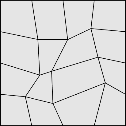
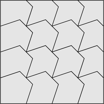
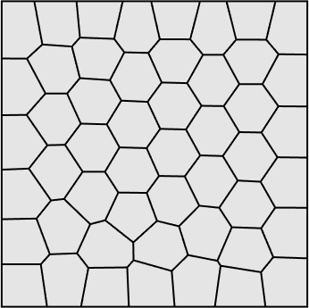
$(a)$	$(b)$	$(c)$

Figure 1: a representative mesh of the three mesh families considered in the test case: $(a)$ distorted squares; $(b)$ nonconvex polygons; $(c)$ Voronoi tesselation.

In this section, we apply the virtual element method developed in the previous sections to the solution of an oscillating circle in two dimensions. For the numerical analysis, domain $\Omega$ is discretized by three different mesh families, respectively composed by distorted squares, nonconvex polygons, and smoothed Voronoi tesselations. Figure 1 shows a representative mesh for each family. The distorted squares and non-convex meshes are based on in-house code developed in Matlab [52]. The two-dimensional polygonal meshes are generated using the built-in Matlab function voronoin and the functions in the modules PolyTop [62] and PolyMesher [63].

Let $e_{h}^{n}=U_{h}^{n}-I_{h}u(t^{n})$ be the error in the approximation of the interpolation of $u(t^{n})$ by the virtual element solution (which is the quantity $\theta^{n}$ that is used in the proof of Theorem 5.1). We measure the relative approximation error according to this definition:

$$\mathcal{E}=\underset{n\in[0,N]}{\max}\mathcal{E}_{0}^{n}+\bigg{(}\Delta t\sum_{n=0}^{N}|\mathcal{E}_{1}^{n}|^{2}\bigg{)}^{\frac{1}{2}}.$$

where

$$\mathcal{E}_{0}^{n}=\left(\frac{m_{h}\big{(}e_{h}^{n},e_{h}^{n}\big{)}}{m_{h}\big{(}I_{h}u(t^{n}),I_{h}u(t^{n})\big{)}}\right)^{\frac{1}{2}}\quad\textrm{and}\qquad\mathcal{E}_{1}^{n}=\left(\frac{a_{h}\big{(}e_{h}^{n},e_{h}^{n}\big{)}}{a_{h}\big{(}I_{h}u(t^{n}),I_{h}u(t^{n})\big{)}}\right)^{\frac{1}{2}}.$$

Before presenting the numerical results, we highlight the implementation process of the new operator which is defined in (32). The major difference with the standard VEM is that we use $\widetilde{\Pi}^{\textsf{E}}$ instead of $\Pi^{0,\textsf{E}}$ in the discretization of the time-derivative term and the right-hand side term. We recall that the former is the orthogonal projector onto the subspace of linear polynomials in every polygonal element with respect to the discrete inner product (20) and the latter is the $L^{2}$ projection operator defined in (6). Our implementation of the local mass matrix on each element E proceeds in three steps. First, we compute the projection matrix

$$\mathbf{\widetilde{\Pi}}^{\textsf{E},\ast}{}=\big{(}\mathsf{D}^{T}\mathsf{D}\big{)}^{-1}\mathsf{D}^{T},$$ (99)

where we recall that $\mathsf{D}$ is the matrix collecting the degrees of freedom of the monomial basis (3) and is defined in (31). Second, we define the elemental mass matrix $\mathsf{M}$ using (99):

$$\mathsf{M}=\big{(}\mathbf{\widetilde{\Pi}}^{\textsf{E},\ast}{}\big{)}^{T}\mathsf{H}\,\mathbf{\widetilde{\Pi}}^{\textsf{E},\ast}{}\quad\textrm{where}\qquad{\mathsf{H}}_{|{ij}}=\int_{\textsf{E}}m_{i}(x,y)m_{j}(x,y)\,dx\,dy\quad i,j=1,2,3.$$

Third, we assemble the global mass matrix as in the standard finite element method. The right-hand side term is also computed using the projection operator $\widetilde{\Pi}^{\textsf{E}}$ in every mesh element. According to (55), we consider

$$\mathbf{b}_{h}=\big{(}\mathbf{\widetilde{\Pi}}^{\textsf{E},\ast}{}\big{)}^{T}\mathbf{f}_{h}\quad\textrm{where}\qquad{\mathbf{f}_{h}}_{|{i}}=\int_{\textsf{E}}m_{i}(x,y)f(x,y)\,dx\,dy.$$

The implementation of the stiffness matrix from the bilinear form $a_{h}(\cdot,\cdot)$ is carried out as usual in the VEM. The primary advantage of using the projection operator $\widetilde{\Pi}^{\textsf{E}}$ is that this operator is computable on the original virtual element space [11], whereas we would need the modified virtual element space [2] to compute the regular $L^{2}$ projection operator $\Pi^{0,\textsf{E}}$.

For the numerical computations, we consider the computational domain $\Omega=[-1,1]^{2}$ and the time interval, $[0,T]=[0,1/2]$. We define the noncontact subdomain $\Omega^{+}(t)$ and the contact set $\Omega^{0}(t)$ as:

$$\Omega^{+}(t)=\big{\{}(x,y)\in\Omega:r(t)>r_{0}(t)\big{\}}\quad\textrm{and}\qquad\Omega^{0}(t)=\big{\{}(x,y)\in\Omega:r(t)\leq r_{0}(t)\big{\}},$$

where $r(t)$ and $r_{0}(t)$ are respectively given by:

$$r(t) =\Big{(}\big{(}x-1/3\cos(4\pi t)\big{)}^{2}+\big{(}y-1/3\sin(4\pi t)\big{)}^{2}\Big{)}^{\frac{1}{2}},$$

$$r_{0}(t) =1/3+0.3\sin(4\pi t).$$

The exact solution $u(x,y,t)$ is given by:

$$u(x,y,t)=\begin{cases}&\dfrac{1}{2}~{}\Big{(}r^{2}(t)-r_{0}^{2}(t)\Big{)}^{2}\quad\text{if}\ (x,y)\in\Omega^{+}(t),\\[5.0pt] &0\hskip 85.78503pt\text{if}\ (x,y)\in\Omega^{0}(t).\end{cases}$$

The initial and boundary conditions can be computed from the exact solution $u(x,y,t)$, see (6). The force function is given by:

$$f(x,y,t)=\begin{cases}\phantom{-}4\Big{[}r_{0}^{2}(t)-2r^{2}(t)-1/2(r^{2}(t)-r_{0}^{2}(t))\Big{(}p(t)+r_{0}(t)~{}r_{0}^{{}^{\prime}}(t)\Big{]}&\quad\text{if}\ (x,y)\in\Omega^{+}(t),\\ -4r_{0}^{2}(t)\Big{[}1-r^{2}(t)+r_{0}^{2}(t)\Big{]}&\quad\text{if}\ (x,y)\in\Omega^{0}(t),\end{cases}$$

Here, $p(t)$ is defined as

$$p(t)=(x-c_{1}(t))c_{1}^{\prime}(t)+(y-c_{2}(t))c_{2}^{\prime}(t),$$

where,

$$c_{1}(t)=\dfrac{1}{3}\cos(4\pi t)\quad\textrm{and}\quad c_{2}(t)=\dfrac{1}{3}\sin(4\pi t)$$

are the centers of the free boundary, which is an oscillatory circle with radius $r_{0}(t)$. It is assumed that the circle is moving with respect to a reference circle of radius $r_{1}$ at the origin. The computations are performed over the three mesh families shown in Figure 1.

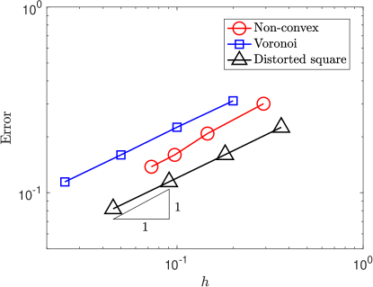
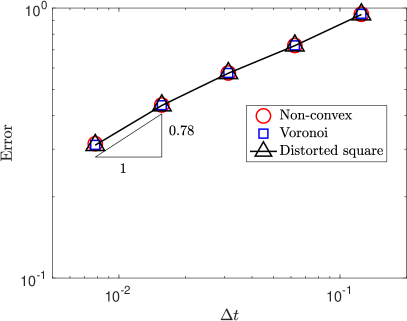
Figure 2: Convergence of the error (see equation (74)) with respect to the mesh refinement for a constant $\Delta t=10^{-3}$ (top panel) and halving $\Delta t=$ on a mesh with fixed $h$ (bottom panel).

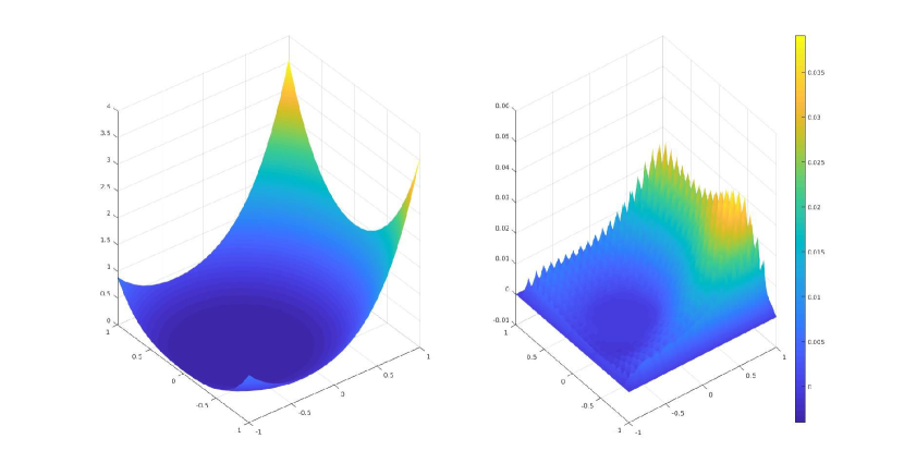
Figure 3: Numerical solution (left panel) and relative approximation error (right panel) $u-u_{h}$ at time $T=.25$.

To study the convergence in space, we consider the time increment $\Delta t=10^{-3}$ and a mesh sequence with initial mesh size as: $(a)$ distorted mesh, $h\approx 0.36$; $(b)$ nonconvex mesh, $h\approx 0.30$; $(c)$ Voronoi tesselation, $h=0.20$. At each mesh refinement we halve $h$. To study the convergence in time, we halve the time step $\Delta t$ at each time refinement starting with $\Delta t=0.125$ and carry out all calculation on the following meshes: $(a)$ distorted square mesh with $h=0.045$; $(b)$ nonconvex mesh with $h=0.073$; $(c)$ Voronoi mesh with $h=0.025$. We choose these mesh sizes in order that the total number of degrees of freedom on the various meshes is almost the same. The convergence of the error with mesh size and time increment is shown in Figures 2 for the three mesh families considered in this test. The triangles close to the error curves show the numerically computed rate of convergence. It can be inferred that the error decreases at the optimal convergence rate in both the space and temporal variable with order $1$ and $\approx 0.75$, respectively, in agreement with Theorem 5.1. Finally, Figure 3 shoes the numerical solution at (left panel) and the corresponding distribution in space of the relative approximation error (right) the final time $T=0.25$.

7 Conclusions

We designed, analyzed and numerically tested a virtual element method for solving the parabolic variational inequality problem in two dimensions over unstructured polygonal meshes. Several aspects make this design challenging. In particular, we used the Maximum and Minimum Principle Theorem to ensure that a virtual element function is nonnegative if all its degrees of freedom are nonnegative. We introduced an approximate orthogonal projector onto linear polynomials, whose approximation properties are carefully investigated in this paper, to compute the mass matrix. The convergence analysis requires a nonnegative quasi-interpolation operator, whose construction on polygonal elements is also discussed in the paper. We proved a convergence theorem and estimated that the convergence rate is proportional to $h$ (the mesh size parameter) and $\Delta t^{\frac{3}{4}}$ (the time step parameter). These results are in perfect agreement with a previous finite element formulation from the literature working in triangular meshes [47]. We assessed the behavior of the VEM against a manufactured solution problem on a two-dimensional domain defined by an oscillating circle using three different polygonal mesh families including distorted squares, nonconvex elements, and Voronoi tesselations. All the numerical convergence rates reflected by the slope of the error curves in our log-log plots agree with the rates that are expected from the theory.

Appendix: An alternative construction of the quasi-interpolation operator

In this section, we would like to outline an alternative proof of Lemma 4.5. For each polygonal element E, we define the quasi-interpolant operator $I_{h}{u}_{|{\textsf{E}}}\in H^{1}(\textsf{E})$ as the solution of the following Poisson’s equation with Dirichlet boundary condition.

$$\Delta I_{h}u =0\phantom{u_{C}}\quad\text{in~{}}\textsf{E},$$

$$I_{h}u =u_{C}\phantom{0}\quad\text{on~{}}\partial\textsf{E},$$

where $u_{C}$ is the Clément interpolation operator on the sub-triangulation of the mesh $\Omega_{h}$ by joining each vertex of $\partial\textsf{E}$ with with the barycentre of E. Following [55], it can be proved that $I_{h}u$ approximates $u$ optimally, i.e.

$$\|u-I_{h}u\|_{0,\textsf{E}}+h_{\textsf{E}}\|u-I_{h}u\|_{1,\textsf{E}}\leq Ch_{\textsf{E}}^{2}|u|_{2,\textsf{E}}.$$

Furthermore, from the construction, on each node $\nu$, $I_{h}u(\nu)=u_{C}(\nu)$, and

$$u_{C}(\nu)=\frac{1}{|\omega_{\nu}|}\int_{\omega_{\nu}}u\,d\mathbf{x},$$

where $\omega_{\nu}$ is the patch of the node $\nu$ on the sub-triangulation of $\Omega_{h}$. Consequently, we have $I_{h}u(\nu)\geq 0$, when $u\geq 0$ almost everywhere on $\Omega$. Moreover, $I_{h}u$ is a harmonic function. Therefore, from corollary (3.2), we emphasize that $I_{h}u\in\mathcal{K}_{h}$ if $u\in\mathcal{K}$.

References

- [1] R. A. Adams and J. J. F. Fournier. Sobolev spaces. Pure and Applied Mathematics. Academic Press, 2 edition, 2003.
- [2] B. Ahmad, A. Alsaedi, F. Brezzi, L. D. Marini, and A. Russo. Equivalent projectors for virtual element methods. Computers & Mathematics with Applications, 66:376–391, September 2013.
- [3] W. Allegretto, Y. Lin, and H. Yang. Finite element error estimates for a nonlocal problem in American option valuation. SIAM Journal on Numerical Analysis, 39(3):834–857, 2001.
- [4] P. F. Antonietti, L. Beirão da Veiga, D. Mora, and M. Verani. A stream virtual element formulation of the Stokes problem on polygonal meshes. SIAM Journal on Numerical Analysis, 52(1):386–404, 2014.
- [5] P. F. Antonietti, L. Beirão da Veiga, S. Scacchi, and M. Verani. A virtual element method for the Cahn-Hilliard equation with polygonal meshes. SIAM Journal on Numerical Analysis, 54(1):34–56, 2016.
- [6] P F. Antonietti, L. Beirão da Veiga, and M. Verani. An adaptive MFD method for the obstacle problem. In Numerical mathematics and advanced applications 2011, pages 3–12. Springer, Heidelberg, 2013.
- [7] P. F. Antonietti, L. Beirão da Veiga, and M. Verani. A mimetic discretization of elliptic obstacle problems. Math. Comp., 82(283):1379–1400, 2013.
- [8] P. F. Antonietti, S. Berrone, M. Verani, and S. Weisser. The virtual element method on anisotropic polygonal discretizations. In Numerical mathematics and advanced applications - ENUMATH 2017, volume 126 of Lect. Notes Comput. Sci. Eng., pages 725–733. Springer, Cham, 2019.
- [9] B. Ayuso de Dios, K. Lipnikov, and G. Manzini. The nonconforming virtual element method. ESAIM: Mathematical Modelling and Numerical Analysis, 50(3):879–904, 2016.
- [10] C. Baiocchi and A. Capelo. Variational an Quasivariational Inequalities. John Wiley and Sons, New York, 1984.
- [11] L. Beirão da Veiga, F. Brezzi, A. Cangiani, G. Manzini, L. D. Marini, and A. Russo. Basic principles of virtual element methods. Mathematical Models & Methods in Applied Sciences, 23:119–214, 2013.
- [12] L. Beirão da Veiga, F. Brezzi, L. D. Marini, and A. Russo. Virtual element method for general second-order elliptic problems on polygonal meshes. Mathematical Models & Methods in Applied Sciences, 26(04):729–750, 2016.
- [13] L. Beirão da Veiga, K. Lipnikov, and G. Manzini. Arbitrary-order nodal mimetic discretizations of elliptic problems on polygonal meshes. SIAM Journal on Numerical Analysis, 49(5):1737–1760, 2011.
- [14] L. Beirão da Veiga, K. Lipnikov, and G. Manzini. The Mimetic Finite Difference Method for Elliptic Problems, volume 11. Springer, 2014.
- [15] L. Beirão da Veiga, C. Lovadina, and G. Vacca. Virtual elements for the Navier-Stokes problem on polygonal meshes. SIAM Journal on Numerical Analysis, 56(3):1210–1242, 2018.
- [16] L. Beirão da Veiga and G. Manzini. Residual a posteriori error estimation for the virtual element method for elliptic problems. ESAIM: Mathematical Modelling and Numerical Analysis, 49(2):577–599, 2015.
- [17] L. Beirão da Veiga, G. Manzini, and L. Mascotto. A posteriori error estimation and adaptivity in virtual elements. Numerische Mathematik, 143, 9 2019.
- [18] L. Beirão da Veiga, D. Mora, and G. Vacca. The Stokes complex for virtual elements with application to Navier-Stokes flows. Journal of Scientific Computing, 81(2):990–1018, 2019.
- [19] M. A. Bencheikh Le Hocine, S. Boulaaras, and M. Haiour. An optimal –error estimate for an approximation of a parabolic variational inequality. Numerical Functional Analysis and Optimization, 37:1–18, 01 2016.
- [20] E. Benvenuti, A. Chiozzi, G. Manzini, and N. Sukumar. Extended virtual element method for the Laplace problem with singularities and discontinuities. Computer Methods in Applied Mechanics and Engineering, 356:571–597, 2019.
- [21] A. E. Berger and R. S. Falk. An error estimate for the truncation method for the solution of parabolic obstacle variational inequalities. Mathematics of Computation, pages 619–628, 1977.
- [22] J. E. Bishop. A displacement based finite element formulation for general polyhedra using harmonic shape functions. International Journal on Numerical Methods in Engineering, 97:1–31, 2014.
- [23] J. F. Blowey and C. M. Elliott. Curvature dependent phase boundary motion and parabolic double obstacle problems. In W.-M. Ni, L. A. Peletier, and J. L. Vazquez, editors, Degenerate Diffusions, pages 19–60, New York, NY, 1993. Springer New York.
- [24] J. H. Bramble and S. R. Hilbert. Estimation of linear functionals on Sobolev spaces with application to Fourier transforms and spline interpolation. SIAM Journal on Numerical Analysis, 7(1):112–124, 1970.
- [25] H. Brezis. Problèmes unilatéraux. Journal des Mathématiques Pures et Appliquées, 52:1–168, 1972.
- [26] F. Brezzi, A. Buffa, and K. Lipnikov. Mimetic finite differences for elliptic problems. ESAIM: Mathematical Modelling and Numerical Analysis, 43(2):277–295, 2009.
- [27] F. Brezzi, R. S. Falk, and L. D. Marini. Basic principles of mixed virtual element methods. ESAIM: Mathematical Modelling and Numerical Analysis, 48(4):1227–1240, 2014.
- [28] E. Cáceres and G. Gatica. A mixed virtual element method for the pseudostress-velocity formulation of the Stokes problem. IMA Journal of Numerical Analysis, 37(1):296–331, 2017.
- [29] A. Cangiani, E. H. Georgoulis, T. Pryer, and O. J. Sutton. A posteriori error estimates for the virtual element method. Numerische Mathematik, 137(4):857–893, 2017.
- [30] A. Cangiani, V. Gyrya, and G. Manzini. The non-conforming virtual element method for the Stokes equations. SIAM Journal on Numerical Analysis, 54(6):3411–3435, 2016.
- [31] A. Cangiani, G. Manzini, and O. J. Sutton. Conforming and nonconforming virtual element methods for elliptic problems. IMA Journal on Numerical Analysis, 37(3):1317–1354, 2016.
- [32] A. Capatina. Variational Inequalities and Frictional Contact Problems. Advances in Mechanics and Mathematics. Springer, 2014 edition, 2014.
- [33] O. Čertík, F. Gardini, G. Manzini, and G. Vacca. The virtual element method for eigenvalue problems with potential terms on polytopic meshes. Applied Mathematics, 63(3):333–365, 2018.
- [34] B. Cockburn, D. Di Pietro, and A. Ern. Bridging the hybrid high-order and hybridizable discontinuous Galerkin methods. ESAIM: Mathematical Modelling and Numerical Analysis, 50(3):635–650, 2016.
- [35] Y. Deng, F. Wang, and H. Wei. A posteriori error estimates of virtual element method for a simplified friction problem. Journal of Scientific Computing, 83:52, 2020.
- [36] D. A. Di Pietro and J. Droniou. The Hybrid High-Order method for polytopal meshes, volume 19. Springer, 2019.
- [37] D. A. Di Pietro, J. Droniou, and G. Manzini. Discontinuous skeletal gradient discretisation methods on polytopal meshes. Journal of Computational Physics, 355:397–425, 2018.
- [38] D. A. Di Pietro and A. Ern. A hybrid high-order locking-free method for linear elasticity on general meshes. Computer Methods in Applied Mechanics and Engineering, 283:1–21, 2015.
- [39] C. M. Elliott. On a variational inequality formulation of an electrochemical machining moving boundary problem and its approximation by the finite element method. IMA Journal of Applied Mathematics, 25(2):121–131, 03 1980.
- [40] L. C. Evans. Partial Differential Equations. Graduate Studies in Mathematics 19. American Mathematical Society, 1998.
- [41] A. Fetter. -error estimate for an approximation of a parabolic variational inequality. Numerische Mathematik, 50(5):557–565, 1987.
- [42] F. Gardini and G. Vacca. Virtual element method for second-order elliptic eigenvalue problems. IMA Journal of Numerical Analysis, 38(4):2026–2054, 2018.
- [43] G. Gatica, M. Munar, and F. Sequeira. A mixed virtual element method for the Navier-Stokes equations. Mathematical Models & Methods in Applied Sciences, 28(14):2719–2762, 2018.
- [44] D. Gilbarg and N. S. Trudinger. Elliptic Partial Differential Equations of Second Order. Classics in Mathematics 224. Springer-Verlag Berlin Heidelberg, 2 edition, 2001.
- [45] R. Glowinski, J. L. Lions, and R. Tremolières. Numerical Analysis of Variational Inequalities. Elsevier Science Ltd, illustrated edition edition, 1981.
- [46] T. Gudi and P. Majumder. Convergence analysis of finite element method for a parabolic obstacle problem. Journal of Computational and Applied Mathematics, 357:85–102, 2019.
- [47] C. Johnson. A convergence estimate for an approximation of a parabolic variational inequality. SIAM Journal on Numerical Analysis, 13(4):599–606, 1976.
- [48] I. Karatzas and S. E. Shreve. Methods of Mathematical Finance. Springer, corrected edition, 1998.
- [49] I. Kazufumi and K. Kunisch. Parabolic variational inequalities: The Lagrange multiplier approach. Journal de Mathématiques Pures et Appliquées, 85, 2006.
- [50] D. Kinderlehrer and G. Stampacchia. An introduction to variational inequalities and their applications. Pure and applied mathematics, a series of monographs and textbooks 88. Academic Press, 1980.
- [51] K. Lipnikov, G. Manzini, and M. Shashkov. Mimetic finite difference method. Journal of Computational Physics, 257 – Part B:1163–1227, 2014. Review paper.
- [52] MATLAB. version R2020b. The MathWorks Inc., Natick, Massachusetts, 2020.
- [53] K.-S. Moon, R. H. Nochetto, T. Von Petersdorff, and C.-s. Zhang. A posteriori error analysis for parabolic variational inequalities. ESAIM: Mathematical Modelling and Numerical Analysis, 41(3):485–511, 2007.
- [54] D. Mora and G. Rivera. A priori and a posteriori error estimates for a virtual element spectral analysis for the elasticity equations. IMA Journal of Numerical Analysis, 40(1):322–357, 2020.
- [55] D. Mora, G. Rivera, and R. Rodríguez. A virtual element method for the Steklov eigenvalue problem. Mathematical Modelling & Methods in Applied Sciences, 25(08):1421–1445, 2015.
- [56] D. Mora, G. Rivera, and R. Rodríguez. A posteriori error estimates for a virtual element method for the Steklov eigenvalue problem. Computer and Mathematics with Applications, 74(9):2172–2190, 2017.
- [57] J.-F. Rodrigues. Obstacle Problems in Mathematical Physics, volume 114 of Notas De Matematica. Elsevier Science Ltd, 1st edition, 1987.
- [58] J.-F. Rodrigues. The variational inequality approach to the one-phase Stefan problem. Acta Applicandae Mathematicae, 8, 01 1987.
- [59] N. Sharma, A. K. Pani, and K. K. Sharma. Expanded mixed FEM with lowest order RT elements for nonlinear and nonlocal parabolic problems. Advances in Computational Mathematics, 44(5):1537–1571, 2018.
- [60] N. Sukumar and E. A. Malsch. Recent advances in the construction of polygonal finite element interpolants. Archives of Computational Methods in Engineering, 13(1):129, 2006.
- [61] K. Y. Sze and N. Sheng. Polygonal finite element method for nonlinear constitutive modeling of polycrystalline ferroelectrics. Finite Element Analysis and Design, 42(2):107–129, November 2005.
- [62] C. Talischi, G. H. Paulino, A. Pereira, and I. F. Menezes. PolyTop: a Matlab implementation of a general topology optimization framework using unstructured polygonal finite element meshes. Structural and Multidisciplinary Optimization, 45, 2012.
- [63] C. Talischi, G. H. Paulino, A. Pereira, and I. F. M. Menezes. PolyMesher: A general-purpose mesh generator for polygonal elements written in Matlab. Structural and Multidisciplinary Optimization, 45(3):309–328, 2012.
- [64] C Vuik. An -error estimate for an approximation of the solution of a parabolic variational inequality. Numerische Mathematik, 57(1):453–471, 1990.