Pimples reduce and dimples enhance flat dielectric surface image repulsion.

Abstract

Near solid-liquid or liquid-liquid interfaces with dielectric contrast, charged particles interact with the induced polarization charge of the interface. These interactions contribute to an effective self-energy of the bulk ions and mediate ion-ion interactions. For flat interfaces, the self-energy and the mediated interaction are neatly constructed by the image charge method. For other geometries, explicit results are scarce and the problem must be treated via approximations or direct computation. This article provides analytical results, valid to first order in perturbation theory, for the self-energy of particles near a deformed near-flat interface. Explicit formulas are provided for the case of a sinusoidal deformation; generic deformations can then be treated by superposition. In addition to results for the self-energy, the surface polarization charge due to a single ion is presented as a quadrature. The interaction between an ion and the deformed surface is modified by the change in relative distance as well as by the curvature of the surface. Solid walls with a lower dielectric constant than the liquid repel all ions. We show here, however, that the repulsion is reduced by local convexity and enhanced by concavity; dimples are more repulsive than pimples.

I Introduction

The properties of electrolyte solutions can be greatly modified by their interaction with their confining surfaces, particularly in the presence of a mismatch between the properties of the bulk and the bounding material. This is the case for confined electrolytes (Wagner, 1924; Onsager and Samaras, 1934), and more specifically those with graphene or silica substrates (Jurado and Espinosa-Marzal, 2017), in capacitive systems Simon and Gogotsi (2010), in colloidal suspsensions (Sacanna, Kegel, and Philipse, 2007), polyelectrolyte solutions(Shim, Kim, and Jung, 2012), encapsulated or disordered proteins (Cao and Bachmann, 2017; Nott, Craggs, and Baldwin, 2016), and liquid-air interfaces Levin (2009) among others. Features of these systems remain a continuous focus of fundamental and applied research by means of both theoretical and experimental methods as well as investigations in their technological deployment. Possible applications where these properties are important include processes of colloidal stabilization(Vrijenhoek, Hong, and Elimelech, 2001; Hansen and Lowen, 2000), control of surface tension (Levin, 2009), design of electrochemical capacitors(Simon and Gogotsi, 2010), and the use of membranes as ion transfer methods(Shirai et al., 1995; Dilger et al., 1979).

Complex behavior can arise when the interface geometry is modified. Most analytical and numerical investigations assume interfaces with planar or other simple geometries Allen, Hansen, and Melchionna (2001); Messina (2002); dos Santos, Bakhshandeh, and Levin (2011); Jadhao, Solis, and De La Cruz (2012); Arnold et al. (2013); Barros and Luijten (2014); Gan et al. (2015); Shen, Li, and De La Cruz (2017); Wu et al. (2018); Nguyen et al. (2019). It has been shown, however, that the roughness of the interface can have important effects: forces between approaching surfaces are modified(Bhattacharjee, Ko, and Elimelech, 1998; Bowen and Doneva, 2000; Bowen, Doneva, and Stoton, 2002; Bradford and Torkzaban, 2013) and ion distributions can exhibit coupling to a substrate geometry(Wu et al., 2018).

This article provides an evaluation of the contribution to the self-energy of bulk ions due to their interaction with a structured polarizable interface. An ion near the interface creates an induced surface polarization charge that interacts with the ion itself, giving rise to this self-interaction. For a flat surface, this self-energy can be readily described by the image charge method. In the general case, it can be determined by solving an integral equation. In this investigation, the surface is considered as a deformed plane. The surface polarization and the resulting self-energy are determined to first order in the amplitude of the plane deformations. It is simplest to consider sinusoidal deformations and construct solutions for all other shapes by superposition. The self-energy in the presence of a sinusoidal deformation is analytically expressed, while the surface charge density is presented as a quadrature that can be directly evaluated.

Analysis of electrolyte systems has multiple aspects. It requires consideration of the interaction between ions and the ensuing collective behavior, the steric effects that arise from the presence of a solid wall and the finite size of ions, and, as noted, the electrical interaction between the ions and the interface as well as the ion-ion interaction due to the polarization of the interface. This work is a contribution to the understanding of this third component. The role of the interaction with the dielectric discontinuity is surprisingly rich and challenging. It was first studied by Wagner and Onsager(Wagner, 1924; Onsager and Samaras, 1934). In that work the effects of the surface were described using the image method and it was established that there is always a strong interaction between ions and surface. In more recent work, Levin(Levin, 2009) has analyzed the effect on the surface tension of a liquid-gas interface due to ions localized at the interface. These effects are not immediately captured by mean-field theories, which require modification to include self-energies (Netz and Orland, 2003; Buyukdagli, Manghi, and Palmeri, 2010; Wang, 2010; Wang and Wang, 2013). These examples show that a clear description of the properties of the self-energy of ions near surfaces is a crucial element of progress towards the understanding of these rich and complex systems.

The results of this calculation presented here fulfill several goals. The concrete evaluation of the self-energy provides a direct way to assess the relevance of these effects in concrete situations. As the results are analytical they can be used as a gauge to measure the effectiveness of numerical solutions. They provide a way to incorporate roughness into effective theoretical descriptions of the system and simplified numerical schemes. By identifying the source of the modifications of the self-energy, the results produce heuristic tools for the design of functional structures where variations of local ion populations are important.

The explicit determination of the effects of the surface deformation requires considerable technical steps. It is, therefore, useful to summarize here some central findings. The key result of this analysis is that near a deformed surface, an ion of charge $ve$ acquires an excess self-energy $\Delta U$. This modifies the classical self-energy result $U_{self}\sim q^{2}/z$ when the charge is at a distance $z$ from the surface, as obtained by the classical image charge method. A sinusoidal roughness of the form $h=A\cos(kx+\psi)$, with $x$ running along the surface and $\psi$ a relative phase, produces an excess self-energy described in detail in section V. This explicit form is best understood by looking at its decay away from the surface and at its values very close to the deformation. For the first case, up to some constant numeric factors, an approximate version of the result can be written as

$$\frac{\Delta U}{k_{B}T}\approx\frac{\ell_{B}Ak^{2}}{(kz)^{3/2}}\cos(kx+\psi)\exp(-kz)[4\gamma-\gamma^{2}(kz)].$$ (1)

Here $\ell_{B}=e^{2}/(4\pi\varepsilon_{W}\varepsilon_{0}k_{B}T)$ is the Bjerrum length, $k_{b}T$ the Boltzmann factor, $\varepsilon_{0}$ the vacuum permittivity and $\varepsilon_{W}$ the relative permittivity of the liquid phase. The ratio $\gamma=\Delta\varepsilon/\varepsilon_{I}$ is a factor that indicates the dielectric contrast between the liquid region and substrate, $\Delta\varepsilon$ is the difference in permittivities and $\varepsilon_{I}$ their average. In part, the result is as expected; effects of the roughness follow the pattern of the substrate and decay into the bulk with a characteristic length set by the roughness, namely, the wavelength $\lambda=2\pi/k$. The distance power $z^{-3/2}$ makes the decay region only important near the surface so that for large wavelengths the corrections do not penetrate indefinitely into the liquid bulk. There is, however, a surprising element in the result as well. The two terms in the expression, proportional to $\gamma$ and $\gamma^{2}$, have different signs and functional behavior. The first term reflects, roughly, the direct effect of the topography bringing the surface closer or farther away from the ion. The second is, in essence, proportional to the local curvature of the surface. When ions are very close to the surface, this second term creates en effective reduction in repulsion for ions near the convex crest of the rough substrate while enhancing the repulsion at the concave troughs. These results suggest interesting applications of substrate patterning to enhance or deplete ion populations at specific locations.

The rest of the article is structured as follows. Section V.3 establishes some basic notation and, before any direct calculation, describes the origin of the results that are explicitly determined later on. Section III describes the integral equation for the polarization charge and describes the self-energy computed from interaction with this charge. Section IV develops the perturbative scheme used for the calculation. Key results of the calculation are presented in section V; examples of evaluation of self-energies in specific geometries are provided there as well. Section VI looks in more detail at the results when the point of observation is very close to the surface. Some further conclusions are presented in VII. Details of the evaluation of several expressions are presented in the appendices.

II Geometric effects on polarization.

The role of substrate roughness has been investigated in the context of surface-surface interactions providing modified effective potentials that correct calculations for perfectly flat surfaces (Bhattacharjee, Ko, and Elimelech, 1998; Bowen and Doneva, 2000; Bowen, Doneva, and Stoton, 2002; Bradford and Torkzaban, 2013). The origin of this behavior is easy to understand as the roughness locally modifies the distance between corresponding patches of the interacting surfaces. In the case of where electrolyte ions interact with surfaces a similar issue arises, though the results are a more complicated. Before describing in detail the calculation of the ions’ effective self-energy, it is convenient to discuss the key effects that appear in the result.

The interaction between a single ion and a surface arises from the polarization of the interface between the liquid medium containing the ion and its bounding solid material. The polarization charge appears as the dielectric constants of both media are different. The net electric field $\mathbf{E}$ produced by an ion and the induced surface charges create a polarization field $\mathbf{P}=\varepsilon_{0}\chi\mathbf{E}$ where $\chi$ is the polarizability. The polarization field produces a net surface charge density $\mathbf{\sigma=P}\cdot\mathbf{n}$, with $\mathbf{n}$ the normal to the surface, pointing away from the polarized medium. There is a contribution from each of the media and, as they have different polarization magnitudes, the net surface charge is not zero. If $\alpha$ labels the liquid region where the ion is located and $\beta$ labels the solid region, $\sigma=\chi^{(\alpha)}\mathbf{E^{(\alpha)}}\cdot\mathbf{n}^{(\alpha)}+\chi^{(\beta)}\mathbf{E^{(\beta)}\cdot n^{(\beta)}}=-(\chi^{(\alpha)}\mathbf{E^{(\alpha)}}-\chi^{(\beta)}\mathbf{E^{(\beta)}})\cdot\mathbf{n}^{(\beta)}.$ The field is discontinuous due to the very presence of charge, but the contribution due to the ion is the same across the interface. Therefore, just due to the field of the ion ($\mathbf{E}_{i}$ we have $\sigma=-\Delta\chi\mathbf{E}_{i}\cdot\mathbf{n}$, with $\Delta\chi=\chi^{(\alpha)}-\chi^{(\beta)}$ and $\mathbf{n}$ the normal oriented into the liquid phase. Fig. 1 sketches the effects of geometry on this polarization contribution. In panel (a) the induced polarization just due to the ion field at a flat interface decreases away from the ion due to the increased distance and the reduced alignment of the field and the normal. Near a pimple, as in panel (b), the distance to the surface is smaller, the field is stronger and the polarization is larger. The opposite effect occurs for a dimple, as in panel (c). However, the distance change is not the only effect at play. The field and the normal are further misaligned in the neighborhood of a convex region, as shown in (d), while their alignment is enhanced near concavities as shown in (e).

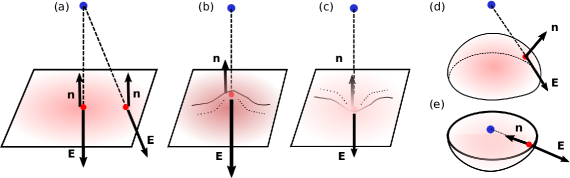
Figure 1: Effects of topographical deformations. (a) The induced surface charge density generated by a single ion is largest at the location closest to the ion. At this point the field is strongest and the normal is aligned with the field direction. (b) At the crest of a deformation, a pimple, the distance is smaller and the field and charge density is larger. (c) At the bottom of a dimple, the field and charge density are smaller. (d) Convexity reduces the polarization misalignment of the normal and the field. (f) Concavity increases the polarization enhancing the alignment.

It is important to remark that for a fixed point in the bulk the presence of a pimple creates both a polarization a enhancement, due to reduced distances, and a decrease due to its convexity; opposite effects arise for the dimple. The explicit calculation below shows that both effects are important. When points with constant height about the average flat plane are considered, the results show a dominant effect due to the decreased or increased local height. However, if one samples the positions above the surface maintaining the local distance to the surface constant, the curvature effect becomes dominant.

The effects noted above have considered only the effect of the direct field created by the ion. The calculation below contains, in addition, all effects due to interaction between the induced charges. The final results show that the heuristics above survive the inclusion of these further interactions. Namely, we still observe that convexity reduces the strength of the interaction while convexity enhances it.

III Integral equation and self-energy

The integral equation for the polarization is well known and is the basis of boundary methods for evaluation of ion interactions in the presence of dielectric media (Allen, Hansen, and Melchionna, 2001; Arnold et al., 2013; Jadhao, Solis, and De La Cruz, 2012; Gan et al., 2015). Here, its structure is reviewed and, along the way, notation is established for the rest of this article. The electric potential $\phi$ created by free charges with density $\rho$ in a polarizable medium is given by the solution of the Poisson equation:

$$\nabla\cdot\varepsilon_{0}\varepsilon\nabla\phi=\rho.$$ (2)

The polarization vector is $\mathbf{P}=\varepsilon_{0}\chi\mathbf{E}=-\varepsilon_{0}\chi\nabla\phi$, so that the volumetric polarization charge density is associated polarization charge is

$$\omega_{v}=\nabla\cdot\mathbf{P}=-\varepsilon_{0}\nabla\cdot\chi\nabla\phi.$$ (3)

The electrostatic energy of the system can be evaluated from the expression

$$U=\frac{1}{2\varepsilon_{0}}\int dV_{r}\int dV_{r^{\prime}}\>\rho(\mathbf{r})G_{r,r^{\prime}}[\rho(\mathbf{r}^{\prime})+\omega_{v}(\mathbf{r}^{\prime})].$$ (4)

Here the geometric Green function is $G(\mathbf{r},\mathbf{r}^{\prime})=[4\pi|\mathbf{r}-\mathbf{r}^{\prime}|]^{-1}$. Inside the integral this is written as $G_{r,r^{\prime}}$. If the charges are considered point-like, their direct self-energy must be subtracted, tough their self-interaction via polarization charges must still be considered and is finite.

The Poisson equation along with the definition of the polarization charge implies an integral equation relation that is useful for explicit computations. This is

$$\omega_{v}(\mathbf{r})=\nabla_{r}\cdot\left[\chi(\mathbf{r})\nabla_{r}\int dV_{r^{\prime}}\,G_{r,r^{\prime}}\left(\omega_{v}(\mathbf{r}^{\prime})+\rho(\mathbf{r}^{\prime})\right)\right].$$ (5)

In the case where the system is composed of piece-wise regions of uniform permittivity, the polarization charge appears only at the location of the point charges, dressing them, and at the interfaces between the uniform regions. For given point charges, this relation becomes a boundary integral equation for the polarization charge.

To make the presentation of the perturbative calculation more transparent it is convenient to present the equation in a way that integral symbols and coordinates are not explicit. A few preliminary steps are required. First, it is assumed that the free charges are point-like, so that the free charge can be written as $\rho(\mathbf{r})=\sum_{i}q_{i}\delta^{3}(\mathbf{r}-\mathbf{r}_{i})$. At each of the locations of the free particles there is polarization charge $\omega_{v}(\mathbf{r})=\omega_{i}\delta^{3}(\mathbf{r}-\mathbf{r}_{i})$ with $\omega_{i}=-\chi_{i}q_{i}/(1+\chi_{i})$ where $\chi_{i}$ is the polarizability at the $i$-th location. The dressed charge at each of these locations is the bare charge $q$ multiplied by the factor $\varepsilon^{-1}.$ That is, $q_{i}+\omega_{i}=\varepsilon_{i}^{-1}q_{i}$. The sum of the charge and its dressing polarization is $\rho(\mathbf{r})+\omega(\mathbf{r})=\sum_{i}\varepsilon_{i}^{-1}q_{i}\delta^{3}(\mathbf{r}-\mathbf{r}_{i})$. Next, the application of the gradient to the integral terms proportional to the surface charge results in two terms. One is proportional to the gradient of the polarization $\nabla\chi=\nabla\varepsilon$. The second is proportional to $\chi\int\nabla_{r}^{2}G_{r,r^{\prime}}\omega(\mathbf{r}^{\prime})=-\chi\omega(\mathbf{r})$. This contribution can be collected on the left hand side to obtain $(1+\chi_{I})\omega=\varepsilon_{I}\omega$. Here, as the permittivity is evaluated at the interface the mean value $\varepsilon_{I}$ must be used.

Collecting the contributions to the integral equation localized at the positions of the free charges leaves only polarization terms associated with the surface polarization. Each interface is assumed smooth and is given an orientation so that a normal vector $\mathbf{n}$ is defined at each of their points. Its direction is the same as that of the gradient $\nabla\varepsilon$ and therefore points towards the region of larger permittivity.

After these constructions, the integral equation can be written as:

$$\omega(\mathbf{r})=\frac{1}{\varepsilon_{0}\varepsilon_{I}}\nabla_{r}\varepsilon\cdot\int dV_{r^{\prime}}\,\nabla_{r}G_{r,r^{\prime}}\left[\omega(\mathbf{r}^{\prime})+\frac{\rho(\mathbf{r}^{\prime})}{\varepsilon_{r^{\prime}}}\right].$$ (6)

Here $\omega$ is the total polarization excluding the contributions dressing the free charges. The polarization $\omega$ is a volumetric density localized at a surface so that, in a flat plane, say $z=0$, is locally proportional to a delta function $\delta(z)$. Below, by abuse of notation, the variable $\omega$ will also be used as the surface charge density that does not include the delta function and, schematically, an abstract vector on which integral operators act. The symbol $\gamma$ will be used for the factor that appears at the interface between media:

$$\gamma=\frac{\Delta\varepsilon}{\varepsilon_{I}}$$ (7)

where $\varepsilon_{I}$ is the mean value of permittivity at an interface and $\Delta\varepsilon$ is the difference in relative permittivities. In the general case, each interface can have a different value of this parameter but in the analysis below there is only one interface and a single value. The liquid region $\alpha$ is considered to have larger relative permittivity. The normal therefore points into the region $\alpha$ and $\gamma$ is positive.

The integral equation can be more succinctly presented as a linear operator equation of the form

$$\omega=\mathcal{B}\omega+\mathcal{H}\rho.$$ (8)

In this expression, $\omega$ is to be understood as a function defined on the interfaces and excludes any contribution from the polarization of the free charges. The surface operator $\mathcal{B}$ describes the interaction between polarization between charges at the boundary between homogeneous regions. The direct interaction operator $\mathcal{\mathcal{H}}$ computes the effect at the surface due to charges in the homogeneous media. The surface operator integrates the surface density times a kernel $B(\mathbf{s},\mathbf{s}^{\prime})$, where $\mathbf{s}$ and $\mathbf{s}^{\prime}$ are three-dimensional coordinates indicating positions of surface points. For readability, the shorthand $B_{s,s^{\prime}}$ is used in several locations below. Explicitly,

$$\mathcal{B}\omega = \int dS_{s^{\prime}}B(\mathbf{s},\mathbf{s}^{\prime})\omega(\mathbf{s}^{\prime})$$ (9)

$$B(\mathbf{s},\mathbf{s}^{\prime}) = \gamma_{s}\mathbf{n}_{s}\cdot\nabla_{s}G(\mathbf{s},\mathbf{s}^{\prime})$$ (10)

Here $dS$ indicates the surface area differential. The explicit form of the direct polarization operator $\mathcal{H}$ is a volumetric integration with kernel $H_{s,r}=H(\mathbf{s},\mathbf{r})$, where the variables used emphasize that the integration is over the charge distribution in space and the result is observed at a surface point. This is

$$\mathcal{H}\rho = \int dV_{r^{\prime}}H(\mathbf{s},\mathbf{r}^{\prime})\rho(\mathbf{r}^{\prime})$$ (11)

$$H(\mathbf{s},\mathbf{r}^{\prime}) = \gamma_{s}\mathbf{n}_{s}\cdot\nabla_{s}G(\mathbf{s},\mathbf{r}^{\prime})\frac{1}{\varepsilon_{r^{\prime}}}$$ (12)

Next, a potential operator $\mathcal{G}$ is defined by integrating the geometric factor $G_{r,s}=G(\mathbf{r},\mathbf{s})$ against a surface charge distribution.

$$\mathcal{G}\omega = \int dS_{s}G(\mathbf{r},\mathbf{s})\omega(\mathbf{s}).$$ (13)

The factor $G(\mathbf{r},\mathbf{s})$ also appears in other expressions in addition to the definition of this operator. The subindices in those cases refer to the evaluation locations.

The second term in the Eq. (4) is the excess energy of the system associated with the polarization of the interface. This is denoted as $U_{p}$, and excludes the direct interactions between bulk charges. Selecting this term only eliminates all singular self-energies of individual ions if they are considered point-like. This is:

$$U_{p}=\frac{1}{2\varepsilon_{0}}\rho^{T}\mathcal{G}\omega.$$ (14)

Here the transpose symbol ^T on the charge density indicates that it is integrated over space against the density $\mathcal{G}\omega$. Furthermore, the main object of interest is the evaluation of this expression in the case of a single point-like charge in the bulk. In that case, $\omega$ is induced by that single charge and the energy appears as a result of its interaction between the induced charge and the bulk charge. This is an induced self-energy and its computation is the main concern of this article.

IV Perturbative scheme

IV.1 General setup

Using a perturbative scheme it is possible to express the self-energy of a single ion and the surface polarization caused by it in the presence of a rough substrate. The scheme expands these quantities as a power series in the amplitude $A$ of the roughness. A dimensionless parameter can be constructed by taking the ratio $A/L$ of the amplitude with respect to the size $L$ of the system. However, the presentation is simplified by working directly with the amplitude. As the operators used depend on the geometry of the surface, they also require expansion. The base geometry is the flat case where all quantities can be exactly evaluated. The results are the closed evaluation of the first order corrections to the resulting surface density and self-energy. The calculation is simplified by the fact that that the boundary operator $\mathcal{B}$ is zero in the flat geometry. The integral equation for the charge density becomes, to first order, a direct evaluation.

The expansion for the polarization $\omega$ is written as

$$\omega=\omega^{(0)}+A\omega^{(1)}+\frac{1}{2}A^{2}\omega^{(2)}\ldots$$ (15)

The superindices in parentheses indicate the order in the expansion. To first order, the expansion for the operators $\mathcal{H}$, $\mathcal{B}$ and $\mathcal{G}$ read

$$\mathcal{H}=\mathcal{H}^{(0)}+A\mathcal{H}^{(1)}+\ldots,$$ (16)

$$\mathcal{B}=\mathcal{B}^{(0)}+A\mathcal{B}^{(1)}+\ldots,$$ (17)

$$\mathcal{G}=\mathcal{G}^{(0)}+A\mathcal{G}^{(1)}+\ldots.$$ (18)

The expansions have a general for but it is already useful to note that in the flat geometry the boundary interaction is zero. This is because it is constructed from the dot product of the electric field between charges in a plane and the normal and these are perpendicular. Namely:

$$\mathcal{B}^{(0)}=\mathcal{B}_{flat}=0.$$ (19)

The self-energy expansion can be written as

$$U_{p}=U_{p}^{(0)}+AU_{p}^{(1)}+\ldots$$ (20)

with a first order factor

$$U_{p}^{(1)}=\frac{1}{2\varepsilon_{0}}\rho^{T}(\mathcal{G}^{(1)}\omega^{(0)}+\mathcal{G}^{(0)}\omega^{(1)}).$$ (21)

The first order correction to the excess self-energy due to the roughness, $\Delta U$, is

$$\Delta U=AU^{(1)}.$$ (22)

The expansion of these quantities and operators are inserted into the integral equation for the Below, the explicit forms of the terms in the operators’ expansions are given. The 0-th order for the equation simply leads to an expression for the charge density as the direct evaluation

$$\omega^{(0)}=\mathcal{H}^{(0)}\rho.$$ (23)

This expression reproduces the image method result. The first order equation for the charge density reduces to

$$\omega^{(1)}=\mathcal{B}^{(1)}\omega^{(0)}+\mathcal{H}^{(1)}\rho=\mathcal{B}^{(1)}\mathcal{G}^{(0)}\rho+\mathcal{H}^{(1)}\rho.$$ (24)

The evaluation of the self energy is

$$U_{p}^{(1)}=\frac{\rho^{T}}{2\varepsilon_{0}}[\mathcal{G}^{(1)}\mathcal{H}^{(0)}+\mathcal{G}^{(0)}\mathcal{H}^{(1)}+\mathcal{G}^{(0)}\mathcal{B}^{(1)}\mathcal{H}^{(0)}]\rho.$$ (25)

As can be seen, the expressions for the polarization charge and self-energy are direct evaluations that do not require any operator inversion.

IV.2 Flat and rough geometries

The geometry of a rough substrate can be described as a deformation of a flat surface. A general roughness pattern can be described as a Fourier superposition of sinusoidal deformations. To first order in the deformation, it is then only necessary to evaluate the effect of such deformations. To this end, we use the coordinate and surface description indicated in Fig. 2. Cartesian coordinates are used with generic point $\mathbf{r}=(x,y,z)$, such that the undeformed surface is located at $z=0.$ Coordinates $(x,y)$ can be used to parameterize both the flat plane and, by projection, the deformed surface. To make some expressions below more readable, the coordinates of points at the surface have a generic three-dimensional coordinate label $\mathbf{s}$. When a point is referred to by its projection to the plane, the generic two-dimensional vector $\mathbf{w}=(x,y)$ is used instead. As all calculations refer only to a single ion; this can be located at a point with coordinates $\mathbf{a}=(0,0,z_{a})$. The deformation shape is described by a normalized height function $h(x,y)$ and absolute height $Ah$.

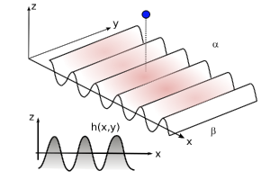
Figure 2: Scheme of the deformed surface. The coordinate system is aligned with undeformed surface which corresponds to $z=0$. The polarizing ion, shown as a small sphere, is in the liquid phase $\alpha$. A sinusoidal deformation is shown with shape $h(x,y)$.

The surface points have deformed surface coordinates $\mathbf{s}$ with the following expansion:

$$\mathbf{s}=\mathbf{s}^{(0)}+A\mathbf{s}^{(1)}+\ldots,$$ (26)

$$\mathbf{s}^{(0)}=(x,y,0),$$ (27)

$$\mathbf{s}^{(1)}=(0,0,h(x,y)).$$ (28)

The main task is to compute the self-energy associated with single wave shapes. These are taken to oscillate along the x-direction so that the height is $A_{0}\cos(kx+\psi)$ for a specific wavevector value $k$ and phase shift $\psi$. This can be written as the real part of a complex exponential with amplitude $A=A_{0}e^{i\psi}$. The calculation is reduced to consideration of plane waves of the form $h=\exp(ikx)$. Below, expressions will use both two- and three-dimensional wavevectors to represent the surface modulation. The three dimensional wave vector is $\mathbf{k}=(k_{x}=k,k_{y}=0,k_{z}=0)$ but the symbol $\mathbf{k}_{2}=(k_{x}=k,k_{y}=0)$ is also used when calculations are carried out explicitly in two dimensions. As noted above, a point in the flat plane has three-dimensional coordinate $\mathbf{s}$ and a two-dimensional representation $\mathbf{w}$. The single plain wave is then $\exp[ikx]=\exp(i\mathbf{k\cdot s})=\exp(i\mathbf{k}_{2}\cdot\mathbf{w})$. integrals.

For a single wave the first order deformation is

$$\mathbf{s}^{(1)}=(0,0,\exp(ikx))=\exp(i\mathbf{k}\cdot\mathbf{s}^{(0)})\hat{\mathbf{z}}.$$ (29)

The deformed surface has normal $\mathbf{n}$ with perturbative expansion

$$\mathbf{n} = \mathbf{n}^{(0)}+A\mathbf{n}^{(1)}+\ldots$$ (30)

$$\mathbf{n}^{(0)} = \hat{\mathbf{z}},$$ (31)

$$\mathbf{n}^{(1)} = -\exp(i\mathbf{k}\cdot\mathbf{s})\hat{\mathbf{x}}=-i\exp(ikx)\mathbf{\hat{\mathbf{x}}}.$$ (32)

Here $\hat{\mathbf{x}}$ and $\mathbf{\hat{z}}$ are unit vectors in the $x$ and $z$ directions. To first order the area differential of the deformed surface remains $dA=d^{2}\mathbf{w}=dx\,dy$.

IV.3 Operator perturbations

The kernels of the operators $\mathcal{B}$, $\mathcal{H}$ and $\mathcal{G}$ have general form as indicated in Eqs. 9, 11, and 13. In the perturbative scheme their 0-th order terms correspond to their values in the flat case. These are:

$$B_{r,r^{\prime}}^{(0)}=0,$$ (33)

$$H_{s,r}^{(0)}=\frac{1}{\varepsilon_{\alpha}}\gamma\frac{1}{4\pi}\frac{(\mathbf{a}-\mathbf{s})\cdot\mathbf{\mathbf{\hat{z}}}}{|\mathbf{a}-\mathbf{s}|^{3/2}}=\frac{\gamma}{4\pi\varepsilon_{\alpha}}\frac{z_{a}}{(z_{a}^{2}+x^{2}+y^{2})^{3/2}},$$ (34)

and

$$G_{s,r}^{(0)}=\frac{1}{4\pi}\frac{1}{|\mathbf{a}-\mathbf{s}|}=\frac{1}{4\pi}\frac{1}{(z_{a}^{2}+x^{2}+y^{2})^{1/2}}.$$ (35)

Next, the first-order terms in the operators’ expansions are obtained by determining the changes in their kernels due to the surface deformation. The deformation changes the relative distance between points and, in the case of the boundary interaction and direct interaction operators the relative direction of the normal. In the case of the geometric Greens function, the change is only due to the modified position of the surface. This is calculated using an operator of the form $\mathbf{s}^{(1)}\cdot\nabla$. In the expressions below, this operator acts only on the Greens function and its derivatives. The deformation of the normal vector is considered separately.

The operator $B_{s,s;}$ is deformed at both positions $s$ and $s^{\prime}$, giving rise to terms $B^{(1a)}$, and $B^{(1b)}$. It also receives a contribution from the change of normal at $w$, namely $B^{(1c)}$.

$$B_{s,s^{\prime}}^{(1)} = B^{(1a)}+B^{(1b)}+B^{(1c)},$$ (36)

$$B_{s,s^{\prime}}^{(1a)} = (\mathbf{s}^{(1)}\cdot\nabla_{s})(\mathbf{n}^{(0)}\cdot\nabla_{s})G_{s,s^{\prime}},$$ (37)

$$B_{s,s^{\prime}}^{(1b)} = (\mathbf{s}^{(1)}\cdot\nabla_{s^{\prime}})(\mathbf{n}^{(0)}\cdot\nabla_{s})G_{s,s^{\prime}},$$ (38)

$$B_{s,s^{\prime}}^{(1c)} = \mathbf{n}^{(1)}\cdot\nabla_{s^{\prime}}G_{s,s^{\prime}}.$$ (39)

Explicitly, these are

$$B_{s,s^{\prime}}^{(1a)} = \frac{\gamma}{4\pi}\frac{\exp(i\mathbf{k}\cdot\mathbf{s}^{\prime})}{|\mathbf{s}-\mathbf{s^{\prime}}|^{3}},$$ (40)

$$B_{s,s^{\prime}}^{(1b)} = \frac{(-\gamma)}{4\pi}\frac{\exp(i\mathbf{k}\cdot\mathbf{s})}{|\mathbf{s}-\mathbf{s}^{\prime}|^{3}},$$ (41)

$$B_{s,s^{\prime}}^{(1c)} = \frac{\gamma}{4\pi}\frac{\mathbf{k}\cdot(\mathbf{s}-\mathbf{s}^{\prime})\exp(i\mathbf{k}\cdot\mathbf{s})}{|\mathbf{s}-\mathbf{s}^{\prime}|^{3}}.$$ (42)

The first-order term for the direct interaction operator has contributions due to the change in position $H^{(1a)}$ and the change in normal orientation $H^{(1b)}$.

$$H_{s,r}^{(1)} = H_{s,r}^{(1a)}+H_{s,r}^{(1b)},$$ (43)

$$H_{s,r}^{(1a)} = \frac{1}{\varepsilon_{r}}\gamma(\mathbf{s}^{(1)}\cdot\nabla)_{s}(\mathbf{n}^{(0)}\cdot\nabla)_{s}G_{w,r},$$ (44)

$$H_{s,r}^{(1b)} = \frac{1}{\varepsilon_{\alpha}}\gamma(\mathbf{n}^{(1)}\cdot\nabla)_{s}G_{s,r}.$$ (45)

Explicitly,

$$H_{s,r}^{(1a)} = \frac{1}{\varepsilon_{\alpha}}\frac{\gamma}{4\pi}\frac{e^{i\mathbf{k}\cdot\mathbf{s}}}{|\mathbf{s}-\mathbf{a}|^{3}}\left[\frac{3(\mathbf{\hat{z}}\cdot\mathbf{\mathbf{a}})^{2}}{|\mathbf{s}-\mathbf{a}|^{2}}-1\right]$$ (46)

$$H_{s,r}^{(1b)} = \frac{1}{\varepsilon_{\alpha}}\frac{\gamma}{4\pi}\frac{e^{i\mathbf{k}\cdot\mathbf{s}}(\mathbf{s}-\mathbf{a})\cdot\mathbf{k}}{|\mathbf{s}-\mathbf{a}|^{3}}.$$ (47)

Finally, the geometric Green function has first order expansion of the form:

$$G_{r,s}^{(1)} = (\mathbf{s}^{(1)}\cdot\nabla_{s})G_{rs},$$ (48)

$$G_{r,s}^{(1)}=\frac{1}{4\pi}\frac{e^{i\mathbf{k}\cdot\mathbf{s}}\mathbf{\mathbf{a}\cdot\hat{\mathbf{z}}}}{|\mathbf{a}-\mathbf{s}|^{3}}.$$ (49)

With these explicit expressions the self-energy and surface polarization density for a single bulk ion are obtained from equations 24, 25 . The first order term for the self-energy is

$$U_{p}^{(1)} = \frac{1}{2\varepsilon_{0}}\rho^{T}[\mathcal{G}^{(1)}\mathcal{H}^{(0)}+\mathcal{G}^{(0)}\mathcal{H}^{(1a)}+\ldots$$ (50)

$$\mathcal{G}^{(0)}\mathcal{H}^{(1b)}+\mathcal{G}^{(0)}\mathcal{B}^{(1a)}\mathcal{H}^{(0)}+\ldots$$

$$\mathcal{G}^{(0)}\mathcal{B}^{(1b)}\mathcal{H}^{(0)}+\mathcal{G}^{(0)}\mathcal{B}^{(1c)}\mathcal{H}^{(0)}]\rho$$

For readability the expression can be presented as

$$U_{p}^{(1)} = \frac{q^{2}}{2\varepsilon_{\alpha}\varepsilon_{0}}[\gamma I_{1}+\gamma I_{2a}+\gamma I_{2b}+\ldots$$ (51)

$$\gamma^{2}I_{3a}+\gamma^{2}I_{3b}+\gamma^{2}I_{3c}],$$

where the $I$ quantities are proportional to the respective terms in the previous equation.

$$\omega^{(1)} = [\mathcal{H}^{(1a)}+\mathcal{H}^{(1b)}+\mathcal{B}^{(1a)}\mathcal{H}^{(0)}+\ldots$$ (52)

$$+\mathcal{B}^{(1b)}\mathcal{H}^{(0)}+\mathcal{B}^{(1c)}\mathcal{H}^{(0)}]\rho.$$

In a more streamlined way the result can be presented as

$$\omega^{(1)}=q[\gamma W_{1a}+\gamma W_{1b}+\gamma^{2}W_{2a}+\gamma^{2}W_{2b}+\gamma^{2}W_{2c}],$$ (53)

with the respective identification of terms in the last two equations.

The expressions for the $I$ and $W$ terms for these last expressions are obtained by surface integrations of the respective integral kernels. Most of the integrations are relatively straightforward, or at least accessible to symbolic manipulations. However, a couple of them require precise rearrangements to cancel singularities in Fourier space, and the use of elliptical coordinates. Therefore, explicit calculations are provided in the appendices. One of the integral expressions for $\omega^{(1)}$ does not appear to be expressible as an analytical form but can be reduced to a quadrature,

V Results

V.1 Flat case

The scheme we use is based on perturbations of the flat system. In the description used, the results for that case are of course identical to the ones obtained by the image method. For an ion of charge $q=Ze$ we have a polarization surface charge

$$\omega_{w}^{(0)}=q\gamma H_{w,s}^{(0)}=q\frac{\gamma}{4\pi\varepsilon_{\alpha}}\frac{\mathbf{a}\cdot\mathbf{\hat{z}}}{|\mathbf{a-\mathbf{s}}|^{3}}.$$ (54)

The self-energy associated with the surface charge is then

$$U_{p}^{(0)}=\frac{1}{8\pi\varepsilon_{0}}\frac{q^{2}}{\varepsilon_{\alpha}}\gamma\frac{1}{4z_{a}},$$ (55)

which is the standard value obtained by the image method. Namely, it reflects the interaction of the charge $q$ with its image $q^{\prime}=\Delta\varepsilon/(2\varepsilon_{I})q=\gamma q/2$, located at a distance $2z_{a}$ from the source. In the context of applications to confined aqueous electrolytes it is useful to note that this energy is always positive, independent of sign charge. This is the case as the liquid phase has larger permittivity than the bounding material so that $\gamma>0$. Dividing by the thermal factor $kT$ the result can also be expressed as

$$\frac{U_{p}}{k_{B}T}=\frac{\ell_{B}}{8}\frac{\gamma Z^{2}}{z_{a}}.$$ (56)

V.2 Self-energy for deformed surface

In the case of the sinusoidal deformation, the self-energy of the ion due to its interaction with the surface is calculated from expression Eq. 51. Remarkably, not only the expression reduces, as noted above, to a direct evaluation, but the required integrals can be evaluated analytically. Using the evaluations obtained in Appendix A, the final and central result of this article is that the excess self-energy for an ion is

$$\Delta U_{p} = A\exp^{ikx}U^{(1)}(k,z)$$ (57)

$$U^{(1)} = \frac{q^{2}}{2\varepsilon_{\alpha}\varepsilon_{0}}\frac{1}{4\pi z^{2}}[\gamma\frac{kz}{4}K_{1}(kz)+\ldots.$$ (58)

$$(-1)\gamma^{2}\frac{(kz)^{2}}{16}K_{0}(kz)]$$

Here $z$ is the elevation of the ion above the mean surface; the subscript (in $z_{a}$) is omitted. The expression uses the modified Bessel functions of 0-th and 1-st order, $K_{0}$ and $K_{1}$ respectively.

The form of the final result indicates that there are two distinct effects created by the surface deformation. The parameter $\gamma$ is in practical applications close to a numerical value of $1$, but the terms proportional to $\gamma$ and $\gamma^{2}$ have different functional behavior. The powers of $\gamma$ appear in the calculation according to the number of surface integrations. The term proportional to $\gamma$ is associated with the interaction of the ion with the direct polarization effect it creates, just as in the classic image case, though accounting for the changes of the relative distance to the wall. The term proportional to $\gamma^{2}$ is associated with the interaction of the ion with the secondary polarization created on the deformed surface due to the direct polarization. This contribution does not appear in the flat case. Evaluation of the term makes clear that it is negative and dominant at high wave-vectors. It is therefore clearly associated with the local curvature of the surface.

Several aspects of the expression obtained require further discussion. First, we note that while the perturbative description is standard, it is not possible to establish its convergence rigorously. Furthermore, there is an important limitation in the description of the self-energy at close distances from the surface, as the region where the ion position $z_{a}$ is within the deformation amplitude $A$, the result is not well defined. A way to recover sensible results in this region is discussed in the next section.

To make the expression obtained more user-friendly, we can consider the region not in the immediate vicinity of the deformation but still within a range where its effects can be felt. For this, we can use the asymptotic form of the modified Bessel functions $K_{\nu}(z)$. For all index $\nu$ this is $K_{\nu}(z)\approx[\pi/(2z)]^{1/2}\exp(-z)$. It is also convenient to measure the energy in thermal units $k_{B}T$ a. The real form of the deformation $A\cos(kx+\psi)$ is directly constructed from the previous result just taking a real part of the complex amplitude result. With these approximations and notation, we can write

$$\frac{\Delta U_{p}}{k_{B}T} = \frac{A}{\ell_{B}}\cos(kx+\psi)\frac{U^{(1)}(k,z)}{k_{B}T}$$ (59)

$$\frac{U^{(1)}}{k_{B}T} = \frac{Z^{2}\ell_{B}}{z^{2}}\frac{\pi^{1/2}}{128^{1/2}}[\gamma(kz)^{1/2}-\gamma^{2}\frac{(kz)^{3/2}}{4}]e^{-kz}$$ (60)

with the numerical constant $C=(pi/128)^{1/2}$. This expression indicates that the effect of the deformation pattern on the self-energy decays into the bulk of the liquid region with a characteristic length equal to the wavelength of the deformation. The effect is further diminished by the inverse powers of the distance $z$ to the surface. The effect of long wavelength deformations is eliminated by these powers.

Results for the full form of the self-energy correction can be readily evaluated. In Figure 3, in the top panel, the self-energy correction is evaluated for different wavevector values and ion locations above the plane. The figure shows energies measured as multiples of the thermal energy scale $kT$ while distances are measured as multiples of Bjerrum lengths, the evaluation corresponds to a location above a crest. For large wavelengths the correction is positive. At small wavelengths, the curvature contribution is negative and can dominate the net result for some values of the ion position. These results agree with the heuristic description of geometric effects of section II. The second panel shows the total self-energy due to polarization, including the flat contribution, for three cases. The ion is considered to be right above a crest, above a trough, and above a flat surface. The deformation considered has amplitude and wavevector $A=0.1\ell_{B}$and $k=1/\ell_{B}$. As can be seen in the example, the correction can be important within the plotted region, within one Bjerrum length.

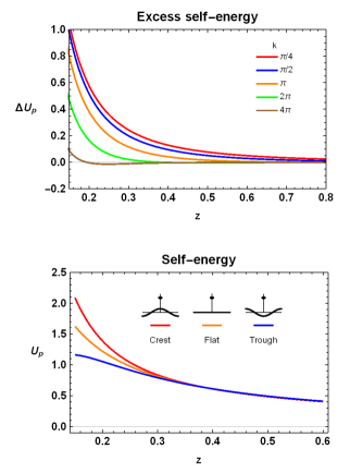
Figure 3: At the top, the excess self-energy $DeltaU_{0}=AU_{p}^{(1)})$ for a single ion as a function of height away from the undeformed surface in the presence of a sinusoidal deformation of amplitude 0.1$\ell_{B}$. The ion is located above a crest. At the bottom, the total self-energy $U_{p}^{(0)}+AU_{p}^{(1)}$ due to surface polarization for the ion in the case of a flat surface, and for positions above a peak and a trough of a surface with sinusoidal deformation with amplitude 0.1$\ell_{B}$ and wavelength $\ell_{B}$. The energies are shown in units of thermal energy and all lengths are measured as multiples of the Bjerrum length.

V.3 Polarization for deformed surface

The polarization surface charge is a function of ion location $\mathbf{a}$ and the observation point at the surface $\mathbf{s}$. In the expressions presented below this variable will stand for the projected location at the surface $(x,y,0)$. Evaluation of the terms for the polarization, as described in the appendix, produces the following result:

$$\omega^{(1)} = \omega_{q}(\mathbf{a},\mathbf{s})+\frac{q}{4\pi\varepsilon_{\alpha}}(\gamma+\frac{1}{2}\gamma^{2})\frac{e^{i\mathbf{k\cdot s}}}{|\mathbf{s}-\mathbf{a}|^{3}}f_{\omega}(\mathbf{a},\mathbf{s})$$ (61)

with

$$\omega_{q}(\mathbf{a},\mathbf{s}) = -\frac{q\gamma^{2}}{4\varepsilon_{\alpha}}e^{i\mathbf{k\cdot\mathbf{s}}}\int\frac{d^{2}\mathbf{p}}{(2\pi)^{2}}e^{i\mathbf{p}\cdot\mathbf{w}}e^{-z_{a}p}|\mathbf{p}+\mathbf{k}_{2}|$$ (62)

and

$$f_{\omega}(\mathbf{a},\mathbf{s})=-1+\frac{3(\hat{\mathbf{z}}\cdot\mathbf{a})^{2}}{|\mathbf{s}-\mathbf{a}|^{2}}+i\mathbf{k}\cdot\mathbf{s}.$$ (63)

The integration defining $\omega_{q}$ is over vectors $\mathbf{p}$ in the two-dimensional space reciprocal to the flat surface. The form of the integral contribution $\omega_{q}$has a succinct form but, as noted in the appendix, it is best to subtract the magnitude $k$ from $|\mathbf{p+\mathbf{k}}_{2}|$ for faster and reliable convergence.

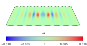
Figure 4: Surface charge density for a surface with a single wave deformation in the presence of a single ion. The ion is located over the central peak at a distance of $\ell_{B}$ from the undeformed surface. The wavelength of the deformation is $\ell_{B}$ and its amplitude is 0.1 $\ell_{B}$. The color plot is superimposed on the deformed surface. Charge density is indicated by color and is presented in units of $e/\ell_{B}^{2}$.

As with the self-energy and for a single-wave surface deformations, the dependence on the ion location is periodic in the direction of the surface oscillation direction. The charge patterns created by ions over crests and troughs are simply the negative of each other. The pattern created when the ion over the lines of zero height, is given by the imaginary part of the expression Eq. 61.

An example of the excess polarization charge, just due to the deformation, for a single-wave deformation appears in Figure 4. The figure shows results for $z_{a}=\ell_{B}$, and $k=2\pi/\ell_{B}$. It can be seen that the pattern decays radially away from the projected ion location and is coupled to both height and curvature. For the parameters chosen, the dominant effect is created by curvature and produces an apparently counterintuitive reduction of the polarization at the central crest. The crest brings the surface closer to the ion and thus increases the local polarization. However, the interaction of the curvature of the deformation with the 0-th order polarization produces a larger negative contribution. The net charge polarization, which includes the $0-th$ order contribution is still positive everywhere; only the correction from the flat case is negative at that location.

V.4 Interaction with a dimple

A Fourier superposition allows the determination of the self-energy of a single ion in the presence of an arbitrary deformation of the surface. As an example, consider a depression on the surface, a “dimple”, with Gaussian form $A\exp[-(x^{2}+y^{2})/2b^{2}]$ relative to its center. The relative position of the dimple center and the ion can be varied to obtain. Using an amplitude of $-0.1\ell_{B}$ and a width $b=1\ell_{B}$ produces the results shown in Fig. 5 for a set of different elevations over the flat plane as a function of the radial distance between dimple center and ion. The dimple creates a reduced self-energy due to the increased distance between ion and surface.

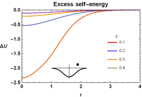
Figure 5: Self-energy for a single ion at different relative radial positions away from a surface dimple. The different lines correspond to fixed elevations away from the unperturbed flat surface. The dimple has a Gaussian shape of depth 0.1$\ell_{B}$ and characteristic width $\ell_{B}$. The excess energy $U$ is measured in thermal units and all lengths are measured as multiples of the Bjerrum length.

VI Results for near approach

As noted above, the results for very small distances from the wall require more careful consideration. The self-energy for point ions near the flat surface becomes infinite. This is easily regularized by introduction of finite size ions and is simply avoided by evaluation away from the interface. However, as the potential is very large near the surface, its gradients are also large and these have been used to evaluate the terms in the perturbative expansion. Therefore, this is not expected to be precise near the deformed surface as is. However, clear results are still recoverable from the perturbative approach by proper treatment of the near-surface region. A key result in this section is the fact that when the set of points at fixed distances from the deformed surface are considered, the heuristic picture described in section II still holds and convex regions produce a negative excess self-energy with the opposite result for concave regions.

To construct a more precise solution near the surface is sufficient to shift the reference plane to the location under consideration. For a given ion location, the reference lane is chosen not as the average undeformed plane but as a plane that exactly matches the surface elevation under the ion. In this way, the ion is at $\mathbf{a}=(0,0,z_{a})$ and the deformation height is $h=0$ at the origin. Instead of the sinusoidal deformation $h(x)=\exp(ikx)$, the shifted form is used:

$$h(x)=\exp(ikx)\,-1.$$ (64)

As written, the deformation consists on the dimpling of the reference plane; all deformations have a negative (real part) height. The self-energy for this configuration is then, simply, the same result as above minus the limit for $k=0$. The result is then

$$\Delta U_{p} = A\cos(kx)U^{(1)}(k,z_{a})$$ (65)

$$U^{(1)}(k,z_{a}) = \frac{q^{2}}{2\varepsilon_{\alpha}\varepsilon_{0}}\frac{1}{4\pi z_{a}^{2}}[\frac{\gamma}{4}\left(kz_{a}K_{1}(kz_{a})-1\right)$$ (66)

$$-\gamma^{2}\frac{(kz_{a})^{2}}{16}K_{0}(kz_{a})]$$

Similarly, if we consider the close approach to a trough, the height profile can be taken as $h(x)=A(1-\exp ikx)$ and the free energy is just the negative of the previous result. Interpolating for all other positions, or by directly repeating these steps for other locations, it is possible to conclude that to first-order, the expression above provides the result for close approach to the surface. These results are consistent with those of the previous section up to differences corresponding to higher orders of the amplitude. Those in the previous section are more useful when exploring the influence of roughness at generic bulk positions. On the other hand, results for close approach allow a clear description of the properties of ions in close contact with the surface.

The expression obtained is quite satisfying. The self-energy of the flat case diverges as $1/z_{a}$ but this correction has, upon expansion at short distances, only a logarithmic $\ln z$ behavior. Namely, the term proportional to $kz(K_{1}(kz)-1)$ is regular at $z=0$ while the second term is proportional to $K_{0}(kz)\approx\ln(z)$. The expression obtained, evaluated near the origin gives the result for a particle near a deformation crest. There, only the term proportional to $\gamma^{2}$ contributes to the self-energy and its value is always negative in that region. In other words, very near the surface, convexity always reduces the strength of the repulsive interaction. By superposition, the peak of a pimple is less repulsive than a flat surface. The analysis is essentially the same for the bottom of the trough, with a change in sign in the amplitude. There, the repulsive interaction is enhanced and the well of a dimple is more repulsive than the flat surface. Evaluation of the self-energy for the crest case is shown in Fig.6.

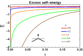
Figure 6: Excess self-energy for a single ion as a function of height away from a sinusoidal peak for different values of the wavevector $k$. The amplitude of the deformation is 0.1$\ell_{B}$. Distances are measure The energy is measured in units of thermal energy and all lengths are measured as multiples of the Bjerrum length. The excess energy is always negative.

VII Conclusions

Possible applications of the results obtained have been outlined in the introduction section. This section discusses previously reported results from simulations of systems with deformed surface geometries, in light of the present work. We indicate possible ways to incorporate the present results into mean field approaches.

Recent work (Wu et al., 2018) reported results from simulations of 1:1 and 2:1 electrolytes confined by a sinusoidally deformed solid boundary. It was observed that in the absence of dielectric contrast between liquid and solid, steric effects reduce the ion population near the surface and that the asymmetric valence case leads to a net charge distribution near the surface favoring the monovalent ions. When no dielectric contrast is present, the ion distribution is not noticeably affected by the shape of the surface; the distributions away from concave and convex features are nearly identical and their differences are well within the fluctuation range of the simulation. In contrast, when the dielectric contrast is turned on, the populations near these features become clearly different. The concave region exhibits a much stronger depletion of multivalent ions compared to monovalent ones. Furthermore, this depletion is stronger at the concave region than at the convex one.

The key features observed in the simulation can be the explained based on the results from this article. Namely, turning on the dielectric contrast between media produces interactions between surface and ions and mediates interactions between the ions. For ions near the surface, the self-energy contribution to the net electric potential is clearly important as it grows with decreasing distance to the surface. This contribution depends on the square of the ions’ valencies, which greatly enhances the asymmetry between species. Both species are repelled from the surface, but the multivalent ions are more strongly repelled, leading in all cases to a net charging of the near-surface region. This net charge density has the same sign as the monovalent species. These observations occur for both flat and deformed surfaces. Corrections to this behavior, due to the deformed geometry, consist of enhancement of ion population near surface peaks and depletion near troughs. These enhancements and depletions are again larger for the multivalent species. Thus, the deformation produces an increase in monovalent sign charge at troughs and a decrease at peaks. As the simulations show, these single ion self-energy effects do not disappear at finite particle density. It is expected, however, that as concentration increases, these effects would weaken due to screening from ion-ion interactions.

The simulations discussed above are computationally expensive and results that can avoid direct computation are of considerable value. Several works have so far incorporated consideration of the self-energy of ions near polarizable surfaces into mean-field approaches to those systems properties. For electrolytes systems, the Poisson-Boltzmann description captures the interaction of ions with the mean field created by surrounding ions, but does not directly include the self-energy contribution. This can be easily seen as the mean field couples to the charge of an ion but, in the conditions discussed, the self-energy is always positive instead of depending on the sign of the valence of the ion. Instead, an extra contribution must be included in the Boltzmann weight, proportional to the exponential of the self-energy ($U_{s}elf$ for a monovalent ion), of the form $\exp[-Z^{2}U_{self}(\mathbf{x})/kT]$. Such approach has been implemented in several previous works where interfaces with dielectric contrast is present, though with simpler geometries (Netz and Orland, 2003; Levin, 2009; Buyukdagli, Manghi, and Palmeri, 2010; Wang, 2010; Wang and Wang, 2013). The results obtained in this article can be incorporated into these mean-field schemes to bridge from the single-ion results obtained here to the case of electrolytes at finite density. As the excess potential is position dependent these contributions contain information about the surface shape and how this influences the region near the surface. When the screening length of the bulk electrolyte is not too small, the features of the surface are observable in the particle distribution, as was shown in the simulations discussed above.

Appendix A Evaluation of first order self-energy terms

The evaluation of the terms that comprise the first order result in the expansion of the self-energy reduce to integrals over space and the flat surface. Most of them can be directly evaluated but a few require limits or coordinate changes that are not trivial. The appendices present the calculations for all terms, but provide more detail in the cases where more technical steps are required.

The self-energy expression is given above in Eq.51 and repeated here:

$$U_{p}^{(1)} = \frac{q^{2}}{2\varepsilon_{\alpha}\varepsilon_{0}}[\gamma I_{1}+\gamma I_{2a}+\gamma I_{2b}+\ldots$$ (67)

$$\gamma^{2}I_{3a}+\gamma^{2}I_{3b}+\gamma^{2}I_{3c}],$$

The terms $I$ contain, in essence, only geometric quantities. The results that follow refer to just these expressions.

The following notation and basic expressions are used. The point ion location is $\mathbf{a}=(0,0,z_{a})$, generic points at the surface are denoted $\mathbf{s}=(x,y,0)$ and $\mathbf{s}^{\prime}=(x^{\prime},y^{\prime},0)$. These three dimensional vectors have two dimensional counterparts $\mathbf{w}=(x,y)$ and $\mathbf{w}^{\prime}=(x^{\prime},y^{\prime})$. The reciprocal vector of a sinusoidal deformation is $\mathbf{k}$. Its two dimensional version is $\mathbf{k}_{2}=(k_{x},k_{y})=(k,0)$. All other reciprocal vectors, used in Fourier representations, are also two dimensional. Most expressions used are derived from two-dimensional Fourier representations of derivatives of electric potentials and field evaluated at the surface. For example, the geometric factor of the normal component $\mathbf{n}\cdot\mathbf{E}$ of the electric field due to a point charge is

$$\frac{1}{4\pi}\frac{\mathbf{\mathbf{z}}\cdot\mathbf{a}}{|\mathbf{a}-\mathbf{s}|^{3}}=\frac{1}{(2\pi)^{2}}\int d^{2}\mathbf{q}\frac{1}{2}e^{-qz_{a}}e^{i\mathbf{q}\cdot\mathbf{w}}$$ (68)

with $q$ the magnitude of the two dimensional reciprocal vector $\mathbf{q}$. As a preliminary result it is also useful to note that for two vectors on the plane, say $\mathbf{w}$, and $\mathbf{w}^{\prime}$, with difference $\Delta\mathbf{w}=\mathbf{w}-\mathbf{w}^{\prime}$, we have

$$\frac{1}{4\pi}\frac{\mathbf{k}\cdot\Delta\mathbf{w}}{|\Delta\mathbf{w}|^{3}}=\lim_{b\rightarrow 0}\frac{1}{(2\pi)^{2}}\int d^{2}\mathbf{q}\frac{\mathbf{q}\cdot\mathbf{k}}{2q}e^{-qb}e^{i\mathbf{q}\cdot\Delta\mathbf{w}}.$$ (69)

Use of this limit form facilitates the handling of cancelling divergent contributions in several expressions below.

A.1 $I_{1}$

This term is the integration of the geometric factors of $G_{r,s}^{(1)}H_{s,r}^{(0)}.$

$$I_{1} = \int dS_{s}\frac{1}{4\pi}\frac{\mathbf{\mathbf{\hat{z}}}\cdot\mathbf{a}\exp(i\mathbf{k}\cdot\mathbf{s})}{|\mathbf{s}-\mathbf{a}|^{3}}\frac{1}{4\pi}\frac{\mathbf{\mathbf{\hat{z}}}\cdot\mathbf{a}}{|\mathbf{s}-\mathbf{a}|^{3}}$$ (70)

$$= \frac{1}{(4\pi)^{2}}\int d^{2}\mathbf{w}\frac{z_{a}^{2}\exp i\mathbf{k}_{2}\cdot\mathbf{w}}{(w^{2}+z_{a}^{2})^{3}}.$$

$$= \frac{1}{(4\pi)}\frac{1}{16z_{a}^{2}}[(kz_{a})^{2}K_{0}(kz_{a})+(kz_{a})K_{1}(kz_{a})].$$

The result is obtained from integration of the angular coordinate in the $\mathbf{w}$ plane, that gives a Bessel function $J_{0}(kw)$. The integration against the factor $w/(w^{2}+z_{a}^{2})^{3}$ gives a result in terms of the Bessel function $K_{2}$, which is then expressed in terms of $K_{0}$ and $K_{1}$.

A.2 $I_{2a}$

This term is the integration of the geometric factors of $G_{r,s}^{(0)}H_{s,r}^{(1a)},.$

$$I_{2a} = \int dS_{s}\frac{1}{4\pi}\frac{1}{|\mathbf{s}-\mathbf{a}|}\frac{1}{4\pi}\frac{\exp(i\mathbf{k}\cdot\mathbf{s})}{|\mathbf{s}-\mathbf{a}|^{3}}[\frac{3(\mathbf{\hat{z}\cdot a})^{2}}{|\mathbf{s}-\mathbf{a}|^{2}}-1]$$ (71)

$$= \frac{1}{(4\pi)^{2}}\int d^{2}\mathbf{w}\frac{\exp i\mathbf{k}_{2}\cdot\mathbf{w}}{(w^{2}+z_{a}^{2})^{2}}\left[\frac{3z_{a}^{2}}{(w^{2}+z_{a}^{2})}-1\right]$$

$$= \frac{1}{16(4\pi z_{a}^{2})}[3(kz_{a})^{2}K_{0}(kz_{a})+kz_{a}K_{1}(kz_{a})]$$

The result is obtained from integration of the angular coordinate in the $\mathbf{w}$ plane resulting on a Bessel function $J_{0}(kr)$. Then, integration against factors $w/(w^{2}+z_{a}^{2})^{2}$, and $w/(w^{2}+z_{a}^{2})^{3}$ gives a result in terms of $K_{1}$ and $K_{2}$. Recursive relations are used to express the result in terms of $K_{0}$and $K_{1}$.

A.3 $I_{2b}$

This term is the integration of the geometric factors of $G_{r,s}^{(0)}H_{s,r}^{(1b)}$.

$$I_{2a} = \int dS_{s}\frac{1}{4\pi}\frac{1}{|\mathbf{s}-\mathbf{a}|}\frac{1}{4\pi}\frac{i\mathbf{s}\cdot\mathbf{k}\exp(i\mathbf{k}\cdot\mathbf{s})}{|\mathbf{s}-\mathbf{a}|^{3}}$$ (72)

$$= \frac{1}{(4\pi)^{2}}\int d^{2}\mathbf{w}\frac{(i\mathbf{k}_{2}\cdot\mathbf{w})e^{i\mathbf{k}_{2}\cdot\mathbf{w}}}{(w^{2}+z_{a}^{2})^{2}}=\frac{1}{4\pi z_{a}^{2}}\frac{\partial}{\partial k}[\frac{k}{4}K_{1}(kz_{a})]$$

$$= \frac{(-1)}{4\pi z_{a}^{2}}\frac{1}{4}kz_{a}K_{0}(kz_{a}).$$

The integrand can be expressed as a derivative with respect to $k$ of a term of the form $\exp ikx/(w^{2}+z_{a}^{2})^{2}$. The integral is a derivative of a multiple of $K_{1}(kz_{a})$. The result follows from the properties of derivatives of the Bessel function.

A.4 $I_{3a}$, $I_{3b}$.

The next two terms are best considered at the same time. These correspond to the factors $G_{r,s}^{(0)}B_{s,s^{\prime}}^{(1a)}H_{s,r}^{(0)}$, and $G_{r,s}^{(0)}B_{s,s^{\prime}}^{(1b)}H_{s^{\prime},r}^{(0)}$.

$$I_{3\alpha} = I_{3a}+I_{3b}$$ (73)

$$= \int dS_{s}\int dS_{s^{\prime}}\left(\frac{1}{4\pi}\right)^{3}\frac{1}{|\mathbf{s}-\mathbf{a}|}\frac{[e^{i\mathbf{k}\cdot\mathbf{s}^{\prime}}-e^{i\mathbf{k}\cdot\mathbf{s}}]}{|\mathbf{s}-\mathbf{s}^{\prime}|^{3}}\frac{\mathbf{\mathbf{\hat{z}}}\cdot\mathbf{a}}{|\mathbf{s}^{\prime}-\mathbf{a}|^{3}}$$

$$= \int\frac{d^{2}\mathbf{w}d^{2}\mathbf{w}^{\prime}}{(4\pi)^{3}}f_{3\alpha}(\mathbf{w},\mathbf{w}^{\prime})$$

with

$$f_{3\alpha}(\mathbf{w},\mathbf{w}^{\prime})=\frac{z_{a}[e^{i\mathbf{k}_{2}\cdot\mathbf{w}^{\prime}}-e^{i\mathbf{k}_{2}\cdot\mathbf{w}}]}{(z_{a}^{2}+w^{2})^{1/2}|\mathbf{w}-\mathbf{w}^{\prime}|^{3}(z_{a}^{2}+w^{\prime 2})^{3/2}}$$ (74)

The integrand has two terms, each the product of three factors with variables $\mathbf{w}$, $\mathbf{w}^{\prime}$ and $\mathbf{w}-\mathbf{w}^{\prime}$. Each factor can be expressed as a two dimensional Fourier integral. The integration over the real space coordinates reduces the integral to the limit of the sum of two terms.

$$I_{3\alpha} =-\displaystyle{\lim_{b\rightarrow 0}}\frac{1}{8b}\int \frac{d^{2}\mathbf{Q}}{(2\pi)^{2}}\left[\frac{e^{-bQ}e^{-z_{a}Q}e^{-z_{a}|\mathbf{Q+\mathbf{k}}_{2}|}}{|\mathbf{Q}+\mathbf{k}_{2}|}\right.$$ (75)

$$\left.-\frac{1}{Q}e^{-bQ}e^{-z_{a}Q}e^{-z_{a}|\mathbf{Q-\mathbf{k}}_{2}|}\right]$$

In the second tern of the integral, the $\mathbf{Q}$ variable shifted to $\mathbf{Q}+\mathbf{k}_{2}$. Then, the limit can be taken to obtain

$$I_{3\alpha} = \int\frac{d^{2}\mathbf{Q}}{8(2\pi)^{2}}\left[\frac{Q}{|\mathbf{Q}+\mathbf{k}_{2}|}-1\right]e^{-z_{a}(Q+|\mathbf{Q}+\mathbf{k}_{2}|)}.$$ (76)

The last expression has two characteristic positions in the $\mathbf{Q}$ plane, namely, the origin and $-\mathbf{k}_{2}$. Factors appearing in the integrand are functions of distances from these two positions. For this reason, a change of variables to elliptic coordinates with loci at the two characteristic locations is natural. These new variables render an integral with known analytical value. The elliptic coordinates are

$$\sigma = \frac{1}{k}(|\mathbf{Q}+\mathbf{k}_{2}|+Q),$$ (77)

$$\tau = \frac{1}{k}(|\mathbf{Q}+\mathbf{k}_{2}|-Q),$$ (78)

The coordinates only cover the upper half plane but by symmetry the integration over the whole plane is twice the value in the half plane. The resulting integral is

$$I_{3\alpha}=\int_{-1}^{1}d\tau\int_{1}^{\infty}d\sigma\frac{k^{2}(-\sigma\tau+\tau^{2})e^{-kz_{a}\sigma}}{8(2\pi)^{2}[(\sigma^{2}-1)(1-\tau^{2})]^{1/2}}$$ (79)

The integrals over each of the variables factorize. The integral over $\tau$ is elementary while the integral over $\sigma$ produces a modified Bessel function. The net result is

$$I_{3\alpha}=\frac{1}{(4\pi)}\frac{1}{16z_{a}^{2}}(kz_{a})^{2}K_{0}(kz_{a}).$$ (80)

A.5 $I_{3c}.$

This integral corresponds to the geometric factors in $G_{r,s}^{(0)}B_{s,s^{\prime}}^{(1c)}H_{s,r}^{(0)}$.

$$I_{3c} = \int dS_{s}\int dS_{s^{\prime}}\frac{1}{(4\pi)^{3}}\frac{1}{|\mathbf{s}-\mathbf{a}|}\frac{i(\mathbf{s}-\mathbf{s}^{\prime})\cdot\mathbf{k}e^{i\mathbf{k}\cdot\mathbf{s}}}{|\mathbf{s}-\mathbf{s}^{\prime}|^{3}}\frac{\mathbf{\mathbf{\hat{z}}}\cdot\mathbf{a}}{|\mathbf{s}^{\prime}-\mathbf{a}|^{3}}$$ (81)

$$= \int\frac{d^{2}\mathbf{w}d^{2}\mathbf{w}^{\prime}}{(4\pi)^{3}}f_{3c}(\mathbf{w},\mathbf{w}^{\prime})$$

with

$$f_{3c}(\mathbf{w},\mathbf{w}^{\prime})=\frac{i\mathbf{k}_{2}\cdot(\mathbf{w-w}^{\prime})z_{a}e^{i\mathbf{k}_{2}\cdot\mathbf{w}}}{(z_{a}^{2}+w^{2})^{1/2}|\mathbf{w}-\mathbf{w}^{\prime}|^{3}(z_{a}^{2}+w^{\prime 2})^{3/2}}$$ (82)

As in the previous evaluation, the factors can be written as Fourier integrals and the integration over real space can be carried out. This leads to a single two dimensional integral in reciprocal space:

$$I_{3c}=\int\frac{d^{2}\mathbf{Q}}{8(2\pi)^{2}}\frac{1}{|\mathbf{Q}+\mathbf{k}_{2}|}\frac{\mathbf{Q}\cdot\mathbf{k}_{2}}{Qk}e^{-z_{a}Q}e^{-z_{a}|\mathbf{Q}+\mathbf{k}_{2}|}.$$ (83)

Elliptical coordinates can again be used to obtain

$$I_{3c}=\int_{-1}^{1}d\tau\int_{1}^{\infty}d\sigma\frac{k^{2}(-1+\sigma\tau)e^{-kz_{a}\sigma}}{8(2\pi)^{2}[(\sigma^{2}-1)(1-\tau^{2})]^{1/2}}.$$ (84)

The final evaluation produces again a result expressable as a Bessel function:

$$I_{3c}=-\frac{1}{4\pi z_{a}^{2}}(kz_{a})^{2}K_{0}(z_{a}k).$$ (85)

Appendix B Evaluation of polarization surface charge density.

The first order correction to the surface charge density is expressed as

$$\omega^{(1)}=qA[\gamma W_{1a}+\gamma W_{1b}+\gamma^{2}W_{2a}+\gamma^{2}W_{2b}+\gamma^{2}W_{2c}].$$ (86)

This appendix describes the evaluation of the terms that appear in this equation.

B.1 $W_{1a}$

This term is the change in the direct polarization contribution due to surface deformation, namely, $H_{s,r}^{(1a)}.$ This is

$$W_{1a} = \frac{1}{4\pi}\frac{\exp[i\mathbf{k\cdot s}]}{|\mathbf{s}-\mathbf{a}|^{3}}\left[-1+\frac{3(\hat{\mathbf{z}}\cdot\mathbf{a})^{2}}{|\mathbf{s}-\mathbf{a}|^{2}}\right]$$ (87)

B.2 $W_{1b}$

This term is simply the evaluation of the geometric factors in the change in the direct effect of the point charge on the deformed surface due to its change in elevation, $H_{s,r}^{(1b)}.$ This is

$$W_{1b} =H_{w,a}^{(1)}= \frac{1}{4\pi}\frac{i\mathbf{k\cdot s}\exp(i\mathbf{k}\cdot\mathbf{s})}{|\mathbf{s}-\mathbf{a}|^{3}}$$ (88)

B.3 $W_{2a}$, $W_{2b}$

These two terms are again best considered at the same time. They correspond to the geometric factors in $B_{s,s^{\prime}}^{(1a)}H_{s^{\prime},r}^{(0)}$, and $B_{s,s^{\prime}}^{(1b)}H_{s^{\prime},r}^{(0)}$.

$$W_{2a}+W_{2b} = \int dS_{s^{\prime}}\frac{1}{4\pi}\frac{[e^{i\mathbf{k}\cdot\mathbf{s}^{\prime}}-e^{i\mathbf{k}\cdot\mathbf{s}}]}{|\mathbf{s}-\mathbf{s}^{\prime}|^{3}}\frac{1}{4\pi}\frac{\mathbf{\mathbf{\hat{z}}}\cdot\mathbf{a}}{|\mathbf{s}^{\prime}-\mathbf{a}|^{3}}.$$ (89)

$$= \int\frac{d^{2}\mathbf{w}}{(4\pi)^{2}}\frac{z_{a}[e^{i\mathbf{k}_{2}\cdot\mathbf{w}^{\prime}}-e^{i\mathbf{k}_{2}\cdot\mathbf{w}}]}{|\mathbf{w}-\mathbf{w}^{\prime}|^{3}\left[z_{a}^{2}+w^{2}\right]^{3/2}}.$$

The factors in the integrand can be presented as Fourier transforms. Integration over the surface leads to an integral in reciprocal space:

$$W_{2a}+W_{2b} = W_{2\alpha}+W_{2\beta}$$

$$W_{2\alpha} = \int\frac{d^{2}\mathbf{Q}}{4(2\pi)^{2}}Qe^{i(\mathbf{Q+\mathbf{k}_{2}})\cdot\mathbf{w}}e^{-z_{a}Q}.$$

$$W_{2\beta} = \int\frac{d^{2}\mathbf{Q}}{4(2\pi)^{2}}|\mathbf{Q}+\mathbf{k}_{2}|e^{i(\mathbf{Q+\mathbf{k}_{2}})\cdot\mathbf{w}}e^{-z_{a}Q}.$$ (90)

To obtain the previous expressions, shifts in the reciprocal variable similar to those in the computation of the $I_{2}$ terms are employed. The first integral is proportional to the derivative with respect to $z_{a}$ of the representation Eq. 68 of the normal component of the electric field in the plane. This gives:

$$W_{2\alpha}=\frac{1}{4\pi}\frac{1}{2}\frac{\exp[i\mathbf{k\cdot s}]}{|\mathbf{s}-\mathbf{a}|^{3}}\left[-1+\frac{3(\hat{\mathbf{z}}\cdot\mathbf{a})^{2}}{|\mathbf{s}-\mathbf{a}|^{2}}\right]$$ (91)

where the expression is again presented in terms of the three dimensional coordinate $\mathbf{s}$.

The second integral $W_{2\beta}$ does not appear to have a closed form expression. In the main text this expression gives rise to the term denoted as the remaining quadrature $\omega_{q}$. It is useful to note that, in numerical evaluations this integral is best computed using a finite region that is centered at $\mathbf{Q=-k}$. In the integral the factor $\mathbf{|Q}+\mathbf{k}|$ can be written as the sum of the terms $(\mathbf{|Q}+\mathbf{k}|-k)$ and $k$. The first produces an integral that numerically is better behaved while the second can be analytically evaluated.

B.4 $W_{3}$

This term contains the geometric factors in $B_{s,s^{\prime}}^{(1c)}H_{s^{\prime},r}^{(0)}$.

$$W_{2c} = \int dS_{s^{\prime}}\frac{1}{4\pi}\frac{i(\mathbf{s}-\mathbf{s}^{\prime})\cdot\mathbf{k}e^{i\mathbf{k}\cdot\mathbf{s}}}{|\mathbf{s}-\mathbf{s}^{\prime}|^{3}}\frac{1}{4\pi}\frac{\mathbf{\mathbf{\hat{z}}}\cdot\mathbf{a}}{|\mathbf{s}^{\prime}-\mathbf{a}|^{3}}.$$ (92)

$$= \int\frac{d^{2}\mathbf{w}}{(4\pi)^{2}}\frac{i(\mathbf{w}-\mathbf{w}^{\prime})\cdot\mathbf{k}_{2}z_{a}e^{i\mathbf{k}_{2}\cdot\mathbf{w}}}{|\mathbf{w}-\mathbf{w}^{\prime}|^{3}(w^{2}+z_{a}^{2})^{3/2}}.$$

In reciprocal space the integral is

$$W_{2c}=\frac{1}{(2\pi)^{2}}\frac{k}{4}e^{i\mathbf{k}_{2}\cdot\mathbf{w}}\int d^{2}\mathbf{Q}\frac{\mathbf{Q}\cdot\mathbf{k}_{2}}{Qk}e^{i\mathbf{Q}\cdot\mathbf{w}}e^{-z_{a}Q}.$$ (93)

The final result can be obtained by expressing the integrand as a derivative with respect to $x$ component of $\mathbf{w}$. The result can be expressed as

$$W_{2c}=\frac{1}{4\pi}\frac{1}{2}\frac{i\mathbf{k}\cdot\mathbf{s}\exp(i\mathbf{k}\cdot\mathbf{s})}{|\mathbf{s}-\mathbf{a}|^{3}}.$$ (94)

References

- Wagner (1924) C. Wagner, “The surface tension of diluted electrolyte solutions.” PHYSIKALISCHE ZEITSCHRIFT 25, 474–477 (1924).
- Onsager and Samaras (1934) L. Onsager and N. N. Samaras, “The surface tension of debye-hückel electrolytes,” The Journal of Chemical Physics 2, 528–536 (1934).
- Jurado and Espinosa-Marzal (2017) L. Jurado and R. Espinosa-Marzal, “Insight into the electrical double layer of an ionic liquid on graphene,” Scientific Reports 7 (2017), 10.1038/s41598-017-04576-x, cited By 34.
- Simon and Gogotsi (2010) P. Simon and Y. Gogotsi, “Materials for electrochemical capacitors,” Nanoscience and technology: a collection of reviews from Nature journals , 320–329 (2010).
- Sacanna, Kegel, and Philipse (2007) S. Sacanna, W. Kegel, and A. Philipse, “Thermodynamically stable pickering emulsions,” Physical Review Letters 98 (2007), 10.1103/PhysRevLett.98.158301, cited By 161.
- Shim, Kim, and Jung (2012) Y. Shim, H. Kim, and Y. Jung, “Graphene-based supercapacitors in the parallel-plate electrode configuration: Ionic liquids versus organic electrolytes,” Faraday Discussions 154, 249–263 (2012), cited By 58.
- Cao and Bachmann (2017) Q. Cao and M. Bachmann, “Dna packaging in viral capsids with peptide arms,” Soft Matter 13, 600–607 (2017), cited By 5.
- Nott, Craggs, and Baldwin (2016) T. Nott, T. Craggs, and A. Baldwin, “Membraneless organelles can melt nucleic acid duplexes and act as biomolecular filters,” Nature Chemistry 8, 569–575 (2016), cited By 152.
- Levin (2009) Y. Levin, “Polarizable ions at interfaces,” Physical review letters 102, 147803 (2009).
- Vrijenhoek, Hong, and Elimelech (2001) E. M. Vrijenhoek, S. Hong, and M. Elimelech, “Influence of membrane surface properties on initial rate of colloidal fouling of reverse osmosis and nanofiltration membranes,” Journal of membrane science 188, 115–128 (2001).
- Hansen and Lowen (2000) J. Hansen and H. Lowen, “Effective interactions between electric double layers,” Annual Review of Physical Chemistry 51, 209–242 (2000).
- Shirai et al. (1995) O. Shirai, S. Kihara, Y. Yoshida, and M. Matsui, “Ion transfer through a liquid membrane or a bilayer lipid membrane in the presence of sufficient electrolytes,” Journal of Electroanalytical Chemistry 389, 61–70 (1995).
- Dilger et al. (1979) J. P. Dilger, S. McLaughlin, T. J. McIntosh, and S. A. Simon, “The dielectric constant of phospholipid bilayers and the permeability of membranes to ions,” Science 206, 1196–1198 (1979).
- Allen, Hansen, and Melchionna (2001) R. Allen, J.-P. Hansen, and S. Melchionna, “Electrostatic potential inside ionic solutions confined by dielectrics: A variational approach,” Physical Chemistry Chemical Physics 3, 4177–4186 (2001), cited By 96.
- Messina (2002) R. Messina, “Image charges in spherical geometry: Application to colloidal systems,” The Journal of chemical physics 117, 11062–11074 (2002).
- dos Santos, Bakhshandeh, and Levin (2011) A. P. dos Santos, A. Bakhshandeh, and Y. Levin, “Effects of the dielectric discontinuity on the counterion distribution in a colloidal suspension,” The Journal of chemical physics 135, 044124 (2011).
- Jadhao, Solis, and De La Cruz (2012) V. Jadhao, F. J. Solis, and M. O. De La Cruz, “Simulation of charged systems in heterogeneous dielectric media via a true energy functional,” Physical review letters 109, 223905 (2012).
- Arnold et al. (2013) A. Arnold, K. Breitsprecher, F. Fahrenberger, S. Kesselheim, O. Lenz, and C. Holm, “Efficient algorithms for electrostatic interactions including dielectric contrasts,” Entropy 15, 4569–4588 (2013), cited By 30.
- Barros and Luijten (2014) K. Barros and E. Luijten, “Dielectric effects in the self-assembly of binary colloidal aggregates,” Physical review letters 113, 017801 (2014).
- Gan et al. (2015) Z. Gan, H. Wu, K. Barros, Z. Xu, and E. Luijten, “Comparison of efficient techniques for the simulation of dielectric objects in electrolytes,” Journal of Computational Physics 291, 317–333 (2015).
- Shen, Li, and De La Cruz (2017) M. Shen, H. Li, and M. O. De La Cruz, “Surface polarization effects on ion-containing emulsions,” Physical review letters 119, 138002 (2017).
- Wu et al. (2018) H. Wu, H. Li, F. J. Solis, M. Olvera de la Cruz, and E. Luijten, “Asymmetric electrolytes near structured dielectric interfaces,” The Journal of chemical physics 149, 164701 (2018).
- Nguyen et al. (2019) T. D. Nguyen, H. Li, D. Bagchi, F. J. Solis, and M. O. de la Cruz, “Incorporating surface polarization effects into large-scale coarse-grained molecular dynamics simulation,” Computer Physics Communications 241, 80–91 (2019).
- Bhattacharjee, Ko, and Elimelech (1998) S. Bhattacharjee, C.-H. Ko, and M. Elimelech, “Dlvo interaction between rough surfaces,” Langmuir 14, 3365–3375 (1998).
- Bowen and Doneva (2000) W. R. Bowen and T. A. Doneva, “Atomic force microscopy studies of membranes: Effect of surface roughness on double-layer interactions and particle adhesion,” Journal of colloid and interface science 229, 544–549 (2000).
- Bowen, Doneva, and Stoton (2002) W. Bowen, T. Doneva, and J. Stoton, “The use of atomic force microscopy to quantify membrane surface electrical properties,” Colloids and Surfaces A: Physicochemical and Engineering Aspects 201, 73–83 (2002).
- Bradford and Torkzaban (2013) S. A. Bradford and S. Torkzaban, “Colloid interaction energies for physically and chemically heterogeneous porous media,” Langmuir 29, 3668–3676 (2013).
- Netz and Orland (2003) R. R. Netz and H. Orland, “Variational charge renormalization in charged systems,” The European Physical Journal E 11, 301–311 (2003).
- Buyukdagli, Manghi, and Palmeri (2010) S. Buyukdagli, M. Manghi, and J. Palmeri, “Variational approach for electrolyte solutions: From dielectric interfaces to charged nanopores,” Physical Review E 81, 041601 (2010).
- Wang (2010) Z.-G. Wang, “Fluctuation in electrolyte solutions: The self energy,” Physical Review E 81, 021501 (2010).
- Wang and Wang (2013) R. Wang and Z.-G. Wang, “Effects of image charges on double layer structure and forces,” The Journal of chemical physics 139, 124702 (2013).