Phenomenoly of the Hidden SU(2) Vector Dark Matter Model

Abstract

We investigate the phenomenology of an extension of the Standard Model (SM) by a non-abelian gauge group $SU(2)_{HS}$ where all SM particles are singlets under this gauge group, and a new scalar representation $\phi$ that is singlet under SM gauge group and doublet under $SU(2)_{HS}$. In this model, the dark matter (DM) candidates are the three mass degenerate dark photons $A_{i}$ $(i=1,2,3)$ of $SU(2)_{HS}$; and the hidden sector interacts with the (SM) particles through the Higgs portal interactions. Consequently, there will be a new CP-even scalar $\eta$ that could be either heavier or lighter than the SM-like Higgs. By taking into account all theoretical and experimental constraints such as perturbativity, unitarity, vacuum stability, non-SM Higgs decays, DM direct detection, DM relic density, we found viable DM is possible in the range from GeV to TeV. Within the viable parameters space, the both of the triple Higgs coupling and the di-Higgs production at LHC14 could be enhanced or reduced depending on the scalar mixing and the mass of the scalar particle $\eta$.

I Introduction

It is a fact that $27\%$ of the matter in the universe is made out of cold dark matter (CDM). Historically, its existence was proposed as a possible explanation for several astrophysical observations in the cluster of galaxiesZwicky:1933gu . The combined analysis of the Planck satellite 2018 results gives a value of the relic abundance of DM density Aghanim:2018eyx

$$\Omega_{{\rm DM}}h^{2}=0.120\pm 0.001\,,$$ (1)

where $h$ is the reduced Hubble constant and $\Omega_{{\rm DM}}$ denotes the energy density of DM in unit of the critical density. Obviously, the DM candidate must be a stable particle, or at least its lifetime is much larger than the lifetime of the universe, with no direct interaction with the electroweak and strong forces. Its stability can be guaranteed by imposing an appropriate symmetry, which can be discrete or continuous. In addition, it has also to be non-relativistic, i.e. cold as the possibility of hot dark matter (DM) is ruled out by several observations. Among these observations one can list briefly, the pattern of fluctuations in the cosmic microwave background, the so early formation of stars, galaxies, and clusters of galaxies and the weak lensing signals we observe. Thus one should consider going beyond SM physics for possible DM candidates. In the literature, many extensions of the SM have been proposed with the DM being a scalar Deshpande:1977rw , fermion Nath:1996xh or a vector boson Cheng:2002ej ; Hambye:2008bq .

In this work, we consider a model, beyond SM, where DM candidates as a multiplet of massive non-standard spin-1 gauge bosons that interact with the SM through the Higgs portal, which was originally proposed in Hambye:2008bq . This model has the privilege that the stability of the DM particles is guaranteed by the custodial symmetry associated to the gauge symmetry and particle content of the model. This symmetry is favored as one, in this case, does not need to impose any kind of discrete or global symmetry by hand. However, several important features of the model were not investigated due to the non-observation of the Higgs boson at the time of the study. For instances, the measurements of some of the Higgs couplings to a reasonable precision can be used to constrain any heavy scalar state which mixes with the SM-like Higgs boson which will be carried in this work. Additionally, triple Higgs coupling and the Di-Higgs production turn to be so important to shed light on new physics and to understand the electroweak symmetry breaking. All these issues will be investigated in this work. Moreover, we provide the complete explicit analytic expressions of the cross sections of the DM annihilation and co-annihilation different channels that contribute to the thermal relic density at freeze out needed for estimating DM relic density. These expressions were not reported in Hambye:2008bq . Finally, we will report the results related to the branching ratios of several decay modes of the scalars in the model which can be tested in future collider experiments.

The paper is organized as follows. First, we review the model proposed in Hambye:2008bq and discuss the mass eigenstates and their couplings that arise from the scalar potential in section II. Then in section III, we investigate the theoretical and experimental constraints, such as vacuum stability, unitarity, and DM direct detection bound, that can be imposed on the model parameters. In section IV, we consider the lightest gauge vector of the $SU(2)_{HS}$ to be a DM candidate and estimate its relic density by considering all possible allowed annihilation channels as well the coannihilation effects. Next, we carry out a detailed study of the collider phenomenology of the model in section V. Finally, we summarize our results and conclude in section VI. Some relevant formulas and expressions of the effective potential and the cross section contributionss are given in Appendix A and Appendix B, respectively.

II Model

In this study, we consider the proposed model in Hambye:2008bq . The model is based on enlarging the gauge symmetry of the SM to include a non-abelian gauge symmetry, is referred to as $SU(2)_{HS}$, under which all SM particles are singlets. The scalar sector of the model contains a new doublet $\phi$ that is charged under the group $SU(2)_{HS}$ and is singlet under the SM gauge group. The extra gauge bosons, associated to $SU(2)_{HS}$, are denoted by $A^{\mu}$. They couple to the SM only through the Higgs portal ($-\lambda_{m}\phi^{\dagger}\phi H^{\dagger}H$) and do not mix with the SM gauge bosons due to the non-abelian character of $SU(2)_{HS}$ Hambye:2008bq . The Lagrangian of the model can be expressed as

$${\cal L}\supset-\frac{1}{4}F^{\mu\nu}\cdot F_{\mu\nu}+(D_{\mu}\phi)^{\dagger}(D^{\mu}\phi)-\lambda_{m}\phi^{\dagger}\phi H^{\dagger}H-\mu_{\phi}^{2}\phi^{\dagger}\phi-\lambda_{\phi}(\phi^{\dagger}\phi)^{2},$$ (2)

where $D^{\mu}\phi=\big{(}\partial^{\mu}-ig_{\phi}\frac{\tau_{i}}{2}A_{i}^{\mu}\big{)}\phi$ with $g_{\phi}$ is the $SU(2)_{HS}$ gauge coupling; and $\tau_{i}$ are the Pauli matrices. The Higgs potential of the SM is parameterized as: ${\cal L}^{SM}\supset-\mu^{2}H^{\dagger}H-\lambda(H^{\dagger}H)^{2}$ with $H^{T}=(\chi^{+},\frac{1}{\sqrt{2}}[h^{\prime}+i\chi^{0}])$. For suitable choice of the parameters $\mu_{\phi}^{2}$ and $\lambda_{m}$, the gauge symmetry $SU(2)_{HS}$ is spontaneously broken when the vacuum expectation value of $\phi$, $\upsilon_{\phi}$, is not vanishing. After expressing the new doublet in the unitary gauge as

$$\phi=\frac{\upsilon_{\phi}+\eta^{\prime}}{\sqrt{2}}\exp\left\{-i\tau_{k}\frac{\xi_{k}}{\upsilon_{\phi}}\right\}\left(\begin{array}[]{c}0\\ 1\end{array}\right),$$ (3)

one gets

$${\cal L} = {\cal L}_{SM}-\frac{1}{4}F_{\mu\nu}\cdot F^{\mu\nu}+\frac{1}{8}(g_{\phi}\upsilon_{\phi})^{2}A_{\mu}\cdot A^{\mu}+\frac{1}{8}g_{\phi}^{2}A_{\mu}\cdot A^{\mu}\eta^{\prime 2}+\frac{1}{4}g_{\phi}^{2}\upsilon_{\phi}A_{\mu}\cdot A^{\mu}\eta^{\prime}$$ (4)

$$+\frac{1}{2}(\partial_{\mu}\eta^{\prime})^{2}-\frac{\lambda_{m}}{2}(\eta^{\prime}+\upsilon_{\phi})^{2}H^{\dagger}H-\frac{\mu_{\phi}^{2}}{2}(\eta^{\prime}+\upsilon_{\phi})^{2}-\frac{\lambda_{\phi}}{4}(\eta^{\prime}+\upsilon_{\phi})^{4}\,,$$

where $A_{\mu}=UA^{\prime}_{\mu}U^{-1}-\frac{i}{g_{\phi}}[\partial_{\mu}U]U^{-1}$ with $U=\exp\{-i\tau_{k}\xi_{k}/\upsilon_{\phi}\}\in SU(2)_{HS}$. In the $A_{i}^{\mu}$ component space, the Lagrangian ${\cal L}$ in (4) has $SO(3)$ custodial symmetry. As a consequence, the three $A_{i}^{\mu}$ components are degenerate in mass, $m_{A}=g_{\phi}\upsilon_{\phi}/2$, stable and hence can serve as vector DM candidates.

In order to proceed, we need to express ${\cal L}$ in (4) in terms of the mass eigenstates. This can be done after minimizing the scalar potential along both $\phi$ and $H$ directions. Setting $H=\exp\{-i\tau_{k}\chi_{k}/\upsilon\}.(0,\,\frac{1}{\sqrt{2}}[\upsilon+h^{\prime}])^{T}$, where $\upsilon=246\,GeV$ is the usual Higgs vacuum expectation value. By imposing the tadpole conditions $\partial V/\partial h=\partial V/\partial\eta=0$ one finds

$$\mu^{2}=-\lambda\upsilon^{2}-\frac{1}{2}\lambda_{m}\upsilon_{\phi}^{2},\,\mu_{\phi}^{2}=-\lambda_{\phi}\upsilon_{\phi}^{2}-\frac{1}{2}\lambda_{m}\upsilon^{2}.$$ (5)

The $h^{\prime}$-$\eta^{\prime}$ mixing due to the presence of the term of $\lambda_{m}$ in (4), leads to the mass squared matrix

$$M^{2}=\left(\begin{array}[]{cc}2\,\lambda\,\upsilon^{2}&\lambda_{m}\,\upsilon\,\upsilon_{\phi}\\ \lambda_{m}\,\upsilon\,\upsilon_{\phi}&2\,\lambda_{\phi}\,\upsilon_{\phi}^{2}\end{array}\right),$$ (6)

which gives the eigenvalues and the mixing

$$m_{1,2}^{2}=\lambda\upsilon^{2}+\lambda_{\phi}\upsilon_{\phi}^{2}\mp\sqrt{\left(\lambda\upsilon^{2}-\lambda_{\phi}\upsilon_{\phi}^{2}\right)^{2}+\lambda_{m}^{2}\upsilon^{2}\upsilon_{\phi}^{2}},\,t_{2\beta}=\frac{\lambda_{m}\,\upsilon\,\upsilon_{\phi}}{\lambda_{\phi}\,\upsilon_{\phi}^{2}-\lambda\,\upsilon^{2}},$$ (7)

where $t_{2\beta}=\tan 2\beta$. By diagonalizing $M^{2}$, we get the mass eigenstates $h$ and $\eta$ that are defined as

$$\left(\begin{array}[]{c}h\\ \eta\end{array}\right)=\left(\begin{array}[]{cc}c_{\beta}&-s_{\beta}\\ s_{\beta}&c_{\beta}\end{array}\right)\,\left(\begin{array}[]{c}h^{\prime}\\ \eta^{\prime}\end{array}\right),$$ (8)

with $c_{\beta}=\cos\beta,\,s_{\beta}=\sin\beta$. Since the couplings are real, the eigenvalues of the matrix $M^{2}$ are required to be positive definite only if

$$\lambda>0,\,\lambda_{\phi}>0,\,2\lambda_{m}+\sqrt{\lambda\lambda_{\phi}}>0.$$ (9)

In our analysis, we identify the $m_{h}\sim 125\,GeV$ eigenstate to be the SM-like Higgs boson and $\eta$ the other eigenstate, therefore, we have two cases where the SM-like Higgs eiegenstate is the (1) light or the (2) heavy eigenstate. Then, in the first case, the CP-even scalar masses (7) should be written as

$$m_{h,\eta}^{2}=\lambda\upsilon^{2}+\lambda_{\phi}\upsilon_{\phi}^{2}\mp(\lambda_{\phi}\upsilon_{\phi}^{2}-\lambda\upsilon^{2})/c_{2\beta},$$ (10)

with $c_{2\beta}=\cos 2\beta$ and the quartic couplings can be expressed as

$$\lambda=\frac{m_{h}^{2}}{2\upsilon^{2}}\,c_{\beta}^{2}+\frac{m_{\eta}^{2}}{2\upsilon^{2}}\,s_{\beta}^{2},\,\lambda_{\phi}=\frac{m_{h}^{2}}{2\upsilon_{\phi}^{2}}\,s_{\beta}^{2}+\frac{m_{\eta}^{2}}{2\upsilon_{\phi}^{2}}\,c_{\beta}^{2},\,\lambda_{m}=\frac{s_{2\beta}}{2\upsilon\upsilon_{\phi}}\,\left(m_{\eta}^{2}-m_{h}^{2}\right).$$ (11)

In the second case, the CP-even scalar masses are given by (7) are

$$m_{h,\eta}^{2}=\lambda\upsilon^{2}+\lambda_{\phi}\upsilon_{\phi}^{2}\pm(\lambda_{\phi}\upsilon_{\phi}^{2}-\lambda\upsilon^{2})/c_{2\beta},$$ (12)

and the quartic couplings

$$\lambda=\frac{m_{h}^{2}}{2\upsilon^{2}}\,s_{\beta}^{2}+\frac{m_{\eta}^{2}}{2\upsilon^{2}}\,c_{\beta}^{2},\,\lambda_{\phi}=\frac{m_{h}^{2}}{2\upsilon_{\phi}^{2}}\,c_{\beta}^{2}+\frac{m_{\eta}^{2}}{2\upsilon_{\phi}^{2}}\,s_{\beta}^{2},\,\lambda_{m}=\frac{s_{2\beta}}{2\upsilon\upsilon_{\phi}}\,\left(m_{h}^{2}-m_{\eta}^{2}\right).$$ (13)

Clearly, the model can be described by the four free parameters $g_{\phi}$, $\lambda_{\phi}$, $\mu_{\phi}$ and $\lambda_{m}$, or equivalently by $s_{\beta},\,g_{\phi},\,m_{\eta}$ and $\upsilon_{\phi}$, in addition to the SM parameters.

Keeping only terms relevant to our study, in the Lagrangian in the mass eigenstates basis, we can write

$${\cal L} \supset -\frac{1}{4}F_{\mu\nu}\cdot F^{\mu\nu}+\frac{1}{2}m_{A}^{2}A_{\mu}\cdot A^{\mu}-\frac{1}{2}m_{\eta}^{2}\eta^{2}-\frac{1}{2}m_{h}^{2}h^{2}-\left(h\,c_{\beta}+\eta\,s_{\beta}\right)\,\bigg{(}\sum_{f}\frac{m_{f}}{\upsilon}f\overline{f}\bigg{)}$$ (14)

$$+ \bigg{[}\frac{s_{\beta}^{2}}{2\upsilon}\eta^{2}+\frac{c_{\beta}^{2}}{2\upsilon}h^{2}+\frac{s_{2\beta}}{2\upsilon}\eta h+\eta s_{\beta}+hc_{\beta}\bigg{]}\bigg{(}\frac{2m_{W}^{2}}{\upsilon}W_{\mu}^{+}W^{-\mu}+\frac{m_{Z}^{2}}{\upsilon}Z^{\mu}Z_{\mu}\bigg{)}$$

$$+ \bigg{[}\frac{c_{\beta}^{2}}{2\upsilon_{\phi}}\eta^{2}+\frac{s_{\beta}^{2}}{2\upsilon_{\phi}}h^{2}-\frac{s_{2\beta}}{2\upsilon_{\phi}}\eta h+\eta c_{\beta}-hs_{\beta}\bigg{]}\bigg{(}\frac{m_{A}^{2}}{\upsilon_{\phi}}A_{\mu}\cdot A^{\mu}\bigg{)}$$

$$- \frac{1}{6}\rho_{h}h^{3}-\frac{1}{6}\rho_{\eta}\eta^{3}-\frac{1}{2}\rho_{1}\eta^{2}h-\frac{1}{2}\rho_{2}h^{2}\eta.$$

where $f$ denotes the SM fermions and the $\rho$’s parameters represents the CP-even scalar triple coiplings that are given by

$$\rho_{1} = -6\lambda_{\phi}\upsilon_{\phi}c_{\beta}^{2}s_{\beta}+6\lambda\upsilon s_{\beta}^{2}c_{\beta}+\lambda_{m}(\upsilon c_{\beta}^{3}-\upsilon_{\phi}s_{\beta}^{3}-2\upsilon c_{\beta}s_{\beta}^{2}+2\upsilon_{\phi}c_{\beta}^{2}s_{\beta}),$$

$$\rho_{2} = 6\lambda_{\phi}\upsilon_{\phi}s_{\beta}^{2}c_{\beta}+6\lambda\upsilon c_{\beta}^{2}s_{\beta}+\lambda_{m}(\upsilon s_{\beta}^{3}+\upsilon_{\phi}c_{\beta}^{3}-2\upsilon c_{\beta}^{2}s_{\beta}-2\upsilon_{\phi}s_{\beta}^{2}c_{\beta}),$$

$$\rho_{\eta} = 6\lambda_{\phi}\upsilon_{\phi}c_{\beta}^{3}+6\lambda\upsilon s_{\beta}^{3}+3\lambda_{m}c_{\beta}s_{\beta}(\upsilon c_{\beta}+\upsilon_{\phi}s_{\beta}),$$

$$\rho_{h} = -6\lambda_{\phi}\upsilon_{\phi}s_{\beta}^{3}+6\lambda\upsilon c_{\beta}^{3}+3\lambda_{m}c_{\beta}s_{\beta}(\upsilon s_{\beta}-\upsilon_{\phi}c_{\beta}).$$ (15)

We notice from (14), that the couplings of $h$ and $\eta$ to SM particles are weighted by $c_{\beta}$ and $s_{\beta}$, respectively. Moreover, in the first case the scalar $\eta$ can additionally decay into Higgs pairs if $m_{\eta}>2m_{h}$ with the partial deacy width

$$\varGamma\,(\eta\rightarrow hh)=\Theta(m_{\eta}-2m_{h})\frac{\rho_{2}^{2}}{32\pi m_{\eta}}\sqrt{1-4\frac{m_{h}^{2}}{m_{\eta}^{2}}},$$ (16)

and in the second case, the Higgs can decay into a pair of $\eta$ if $m_{h}>2\,m_{\eta}$, in addition to their possible decay to $A_{i}A_{i}$.

III Theoretical & Experimental Constraints

This model is subject to a number of theoretical and experimental constraints such as vacuum stability, perturbativity, perturbative unitarity, electroweak precision tests (EWPT), and the constraints from the Higgs decay. For the EWPT, it is expected that the new physics contribution to the oblique parameters ($\Delta S$ and $\Delta T$) is negligeable since the scalar doublet $\eta$ is a singlet the SM gauge group. Then, by considering the constraints from the Higgs signal strenth $\mu_{{\rm tot}}\geq 0.89~{}{\rm at}~{}95\%\,{\rm CL}$ Arcadi:2019lka , the $h-\eta$ mixing makes both $\Delta S$ and $\Delta T$ very tiny, and all the space parameters will be allowed by the EWPT. In what follows, we discuss the above mentioned constraints in details.

• Unitarity constraints

  Possible constraints on the quartic couplings $\lambda$, $\lambda_{\phi}$ and $\lambda_{m}$, can be derived upon requiring that the amplitudes for the scalar-scalar scattering $S_{1}S_{2}\to S_{3}S_{4}$ at high energies respect the tree-level unitarity Cornwall:1974km . Here, $S_{i}$ can be $h$ or $\eta$ for $i=1,2,3,4$. This can be understood as, at high energies, the dominant contributions to these amplitudes are those mediated by the quartic couplings Arhrib:2000is . Denoting the eigenvalues of the scattering matrix as $\Lambda_{i}$, the unitarity condition reads

  $$|\Lambda_{i}|\leq 8\pi$$ (17)

  In the model under concern the above bound results in the following constraints

  $$\lambda_{m}\leq 8\pi,\,\,\,\,\lambda\leq 4\pi,\,\,\,\,\lambda_{\phi}\leq 4\pi,\,\,\,\,3\big{(}\lambda+\lambda_{\phi}\big{)}\pm\sqrt{9\big{(}\lambda-\lambda_{\phi}\big{)}^{2}+4\lambda_{m}^{2}}\leq 8\pi.$$ (18)

• Vacuum Stability and Perturbativity

  The quartic couplings of the scalar potential is subjected to a number of constraints to ensure that the potential is bounded from below and that the couplings remain perturbative as well the electroweak vacuum to be stable all the way up to the Planck scale. For the scalar potential to be bounded from below, the conditions $\lambda>0$, $\lambda_{\phi}>0$ and $\lambda\lambda_{\phi}>0$ must hold and for the case $\lambda_{m}<0$, the condition $2\lambda_{m}+\sqrt{\lambda\lambda_{\phi}}>0$ must be also satisfied. Recall that, one needs $4\lambda\lambda_{\phi}>\lambda_{m}^{2}$ so that the Higgs mixing matrix $M^{2}$ is positive definite and thus $m_{h},m_{\eta}>0$.

• Constraints on the Higgs Decays

  Since the Higgs couplings are modified in our model, and since there exist new particles with new interactions, then the Higgs total decay width and branching ratios get modified. Here, all the vertex of the Higgs-gauge fields and Higgs-fermions are scaled by $c_{\beta}$, therefore the Higgs partial decay widths to the SM paritcles are scaled as $\Gamma(h\rightarrow X_{SM}\bar{X}_{SM})=c_{\beta}^{2}\,\text{$\Gamma$}_{SM}(h\rightarrow X_{SM}\bar{X}_{SM})$. In addition to the SM final states, the Higgs may decay into new gauge bosons ( dark photons) if kinematicaly allowed, with the Higgs partial decay width

  $$\varGamma_{inv}\,(h\rightarrow AA)=\sum_{i=1}^{3}\varGamma\,(h\rightarrow A_{i}A_{i})=3\Theta(m_{h}-2m_{A})\frac{g_{\phi}^{2}\,m_{h}^{3}s_{\beta}^{2}}{64\pi m_{A}^{2}}\sqrt{1-4\frac{m_{A}^{2}}{m_{h}^{2}}}\left\{1-4\frac{m_{A}^{2}}{m_{h}^{2}}+12\frac{m_{A}^{4}}{m_{h}^{4}}\right\},$$ (19)

  this channel is open when $m_{A}<m_{h}/2$. The factor “3” in (19) refers to the summation over $A_{i}A_{i}$. In Case $2$ where the condition $m_{h}>2\,m_{\eta}$ may be fulfilled, the decay channel $h\rightarrow\eta\eta$ is open and the partial width is given by

  $$\varGamma\,(h\rightarrow\eta\eta)=\Theta(m_{h}-2m_{\eta})\frac{\rho_{1}^{2}}{32\pi m_{h}}\sqrt{1-4\frac{m_{\eta}^{2}}{m_{h}^{2}}}.$$ (20)

  Therefore, the Higgs total decay width can be written as

  $$\Gamma_{h}=\text{$\Gamma_{BSM}$}+c_{\beta}^{2}\,\Gamma_{h}^{SM},$$ (21)

  where $\Gamma_{h}^{SM}=4.2~{}\mathrm{MeV}$ is the Higgs total decay width in the SM; $\Gamma_{BSM}=\text{$\Gamma_{inv}$}$ for Case$\,1$; and $\text{$\Gamma_{BSM}$}=\text{$\Gamma_{inv}$+$\Gamma_{und}$}$ for Case$\,2$. Here, the undetermined Higgs decay width $\Gamma_{und}=\Gamma(h\rightarrow\eta\eta)$, which is different than the invisible one at collider; since the light scalar can be seen at detector via the decay to light fermions $\eta\rightarrow f\bar{f}$. These decays do not match the known SM ones, hence, the signal $h\rightarrow\eta\eta\rightarrow f_{1}\bar{f_{1}}f_{2}\bar{f_{2}}$ is named untermined. Then, the invisible and undetermined branching ratio must respect the constarints Aad:2019mbh ; Aaboud:2019rtt

  $$\mathcal{B}_{inv}<0.26,\,\mathcal{B}_{und}<0.22,\,\mathcal{B}_{inv}+\mathcal{B}_{und}\leq 0.47.$$ (22)

  In addition, the Higgs total decay width should lie in the range Khachatryan:2015mma ; Aaboud:2018puo

  $$1.0~{}\mathrm{MeV}<\Gamma_{h}<6.0~{}\mathrm{MeV}.$$ (23)

• DM Direct Detection Constraints

  The DM candidate can interact with nucleons via $t$-channel diagrams that are mediated by h and $\eta$ as shown in Fig. 1.

  

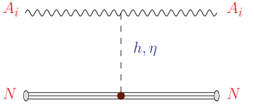
  Figure 1: Feynman diagrams that lead to DM direct detection at underground detectors.

  Measuring nuclear recoil energy resulting from the elastic scattering of DM particle off nucleus in detector can serve as a direct search of DM particles. The results of such searches can be used to impose constraints on the relevant parameters of the model. At tree-level, the spin independent elastic scattering of the vector DM off nucleus, mediated by $h$ or $\eta$ exchange, given in Hambye:2008bq , can be simplifed as

  $$\sigma_{SI}\left(NA\rightarrow NA\right) =\frac{1}{64\pi}f^{2}g_{\phi}^{4}\,s_{2\beta}^{2}m_{N}^{2}\,\frac{\upsilon_{\phi}^{2}}{\upsilon^{2}}\frac{(m_{h}^{2}-m_{\eta}^{2})^{2}}{m_{h}^{4}m_{\eta}^{4}}\left(\frac{m_{N}}{m_{N}+m_{A}}\right)^{2}$$

  $$=6.45765608\times 10^{-42}cm^{2}\,s_{2\beta}^{2}\left(\frac{g_{\phi}}{0.5}\right)^{4}\left(\frac{\upsilon_{\phi}}{100\,\mathrm{GeV}}\right)^{2}\left(\frac{m_{h}}{m_{\eta}}\right)^{4}\left(1-\frac{m_{\eta}^{2}}{m_{h}^{2}}\right)^{2}\left(1+\frac{m_{A}}{m_{N}}\right)^{-2}.$$ (24)

  Here, $m_{N}$ denotes the nucleon mass and $f=0.3$ Hambye:2008bq , parametrizes the Higgs nucleon coupling. This has to be compared with the present experimental upper bound on this cross section Aprile:2015uzo .

• Renormalization Group Equation

  The constraints from vacuum stability and couplings perturbativity can be determined by the renormalisation group evolution of $\lambda,\lambda_{m},\lambda_{\phi}$. At one-loop $\beta$ functions and upon neglecting all the Yukawa couplings except for $y_{t}$, the relevant equations are given as Falkowski:2015iwa ; Arcadi:2019lka :

  $$16\pi^{2}d\lambda/dt = 24\lambda^{2}+2\lambda_{m}^{2}-6y_{t}^{4}+\lambda\,(12y_{t}^{2}-\frac{9}{5}g_{1}^{2}-9g_{2}^{2})+\frac{27}{200}g_{1}^{4}+\frac{9}{20}\,g_{1}^{2}g_{2}^{2}+\frac{9}{8}g_{2}^{4}\;,$$

  $$16\pi^{2}d\lambda_{\phi}/dt = 24\lambda_{\phi}^{2}+2\lambda_{m}^{2}-9\lambda_{\phi}g_{\phi}^{2}+\frac{9}{4}g_{\phi}^{4}\;,$$

  $$16\pi^{2}d\lambda_{m}/dt = \lambda_{m}\,(6y_{t}^{2}+12\lambda+12\lambda_{\phi}+4\lambda_{m}-\frac{9}{10}g_{1}^{2}-\frac{9}{2}g_{2}^{2}-\frac{9}{2}g_{\phi}^{2})\;,$$

  $$16\pi^{2}dg_{i}/dt = b_{i}\,g_{i}^{3}\quad\textrm{with}\quad(b_{1},b_{2},b_{3},b_{\phi})=(41/6,-19/6,-7,-43/6)\;,$$

  $$16\pi^{2}d\lambda_{t}/dt = y_{t}\,(\frac{9}{2}y_{t}^{2}-\frac{17}{20}g_{1}^{2}-\frac{9}{4}g_{2}^{2}-8g_{3}^{2})\;,$$ (25)

  where $g_{i}=(g_{1},g_{2},g_{3})$ represent the SM gauge couplings and $g_{\phi}$ is the gauge coupling of the new $SU(2)_{H}$. In what follows, we will use (25) to check whether the conditions of the vacuum stability, perutrbativity and unitarity are filfilled at higher scales $\Lambda=100\,TeV,\,10^{4}\,TeV$ and $\Lambda=m_{Planck}$.

IV Dark Matter Relic Density

In order to estimate the relic density, one has to estimate the freeze-out temperature and the annihilation cross section. The thermal relic density at freeze out is given in the terms of the thermally averaged annihilation cross section by Srednicki:1988ce :

$$\varOmega_{DM}h^{2}\backsimeq\frac{1.04\times 10^{9}}{M_{pl}}\frac{x_{F}}{\sqrt{g_{*}(x_{F})}}\frac{3}{<\sigma(AA)\upsilon_{r}>},$$ (26)

where $\upsilon_{r}$ is the relative velocity, $M_{pl}=1.22\times 10^{19}\,GeV$ is the Plank mass, $g_{*}$ counts the total number of relativistic degrees of freedom, and $x_{F}=m_{A}/T_{f}$ is the inverse freeze-out temperature. The factor “$3$” in (26) comes from the fact that the total relic density is the summation of the contributions of the three vector bosons $A_{i}$, that have same masses, same interactions, and hence give the same contribution to the relic density. The total thermally averaged annihilation cross section

$$<\sigma(AA)\upsilon_{r}>=\frac{1}{8Tm_{A}^{4}K_{2}^{2}(m_{A}/T)}\sum_{X}\int_{4m_{A}^{2}}^{\infty}ds~{}\sigma_{AA\rightarrow X}(s)\sqrt{s}\left(s-4m_{A}^{2}\right)K_{1}(\sqrt{s}/T),$$ (27)

where $K_{1,2}$ are the modified Bessel functions and $\sigma_{AA\rightarrow X}(s)$ is the annihilation cross section due to the channel $AA\rightarrow X$, at the CM energy $\sqrt{s}$.

The freeze-out parameter $x_{F}$ can be obtained iteratively from the equation:

$$x_{F}=\log\left(\frac{5}{4}\sqrt{\frac{45}{8}}\frac{3}{2\pi^{3}}\frac{M_{pl}m_{A}<\sigma(AA)\upsilon_{r}>}{\sqrt{g_{*}(x_{F})x_{F}}}\right),$$ (28)

where the factor “$3$” in (28) refers to the DM degrees of freedom.

In case where the DM candidate is close in mass to other species, the coannihilation effect becomes important, and in order to take it into account, the thermal average cross section, $<\sigma(AA)\upsilon_{r}>$, in (26) and (28) should be replaced the effective one $\left\langle\sigma_{eff}(AA)\upsilon_{r}\right\rangle$. The effective thermally averaged annihilation cross section is given by Srednicki:1988ce :

$$\begin{array}[]{c}\sigma_{eff}(x)=\sum_{ij}^{N}\frac{g_{i}g_{j}}{g_{eff}^{2}}\sigma_{ij}(1+\Delta_{i})^{3/2}(1+\Delta_{j})^{3/2}\exp[-x(\Delta_{i}+\Delta_{j})],\\ g_{eff}(x)=\sum_{i=1}^{N}g_{i}(1+\Delta_{i})\exp(-x\Delta_{i}),\end{array}$$ (29)

where $\Delta_{i}=\frac{m_{i}-m_{DM}}{m_{DM}}$ and $g_{i}$ is the multiplicity if the species $"i"$. In our model, we consider the co-annihilation effect coming from the mass degeneracy between the vector bosons $A_{i}$, and therefore $g_{i}=3$, $g_{eff}=3$, $\sigma(A_{i}A_{j\neq i})=\sigma(A_{1}A_{2})$ and $\sigma(A_{i}A_{i})=\sigma(A_{1}A_{1})$. Thus, the effective thermally averaged cross section reads:

$$\sigma_{eff}(AA)=\frac{1}{3}[\sigma(A_{1}A_{1}\rightarrow all)+2\sigma(A_{1}A_{2}\rightarrow all)].$$ (30)

In our analysis, we estimate the relic density by considering (26), (28) and (30), and confront it to the recent precise measurements from the PLANCK satellite shown in (1). Here, we consider $3\sigma$ range, i.e., $0.117\leq\Omega_{DM}h^{2}\leq 0.123$. In the rest of this section, we estimate the different contributions to the cross sections $\sigma(A_{1}A_{1})$ and $\sigma(A_{1}A_{2})$.

For the cross section $\sigma(A_{1}A_{1})$, we have many channels: $f\bar{f}$, $WW$, $ZZ$, $hh$, $\eta\eta$ and $h\eta$ as shown in Fig. 2.

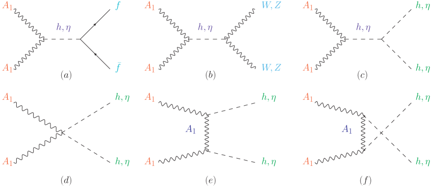
Figure 2: Different DM self-annihilation channels.

While, for the cross section $\sigma(A_{1}A_{2})$, we have only one channel as shown in Fig. 3.

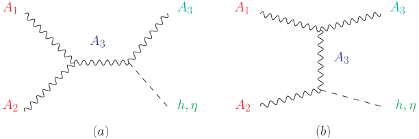
Figure 3: The DM co-annihilation channel.

From the diagram in Fig. 2-a, the annihilation cross section into fermion pairs ($f\bar{f}$) at CM enegy $\sqrt{s}$ is estimated to be

$$\sigma(A_{1}A_{1}\rightarrow bf\bar{f})\upsilon_{r} =N_{c}\frac{s_{2\beta}^{2}}{144\pi}\frac{m_{A}^{4}m_{f}^{2}}{\upsilon_{\phi}^{2}\upsilon^{2}}\,\mathcal{BW}\,\left(1-\frac{4m_{f}^{2}}{s}\right)^{\frac{3}{2}}\left(12-4\frac{s}{m_{A}^{2}}+\frac{s^{2}}{m_{A}^{4}}\right),$$ (31)

$$\mathcal{BW} =\left|\frac{i}{s-m_{h}^{2}+im_{h}\Gamma_{h}}-\frac{i}{s-m_{\eta}^{2}+im_{\eta}\Gamma_{\eta}}\right|^{2},$$ (32)

with $s_{2\beta}=\sin(2\beta)$, $N_{c}$ is the color factor (1 for leptons and 3 for quarks), $\Gamma_{h}$ ($\Gamma_{\eta}$) is the total decay width of the Higgs (scalar $\eta$).

The annihilation cross section into gauge bosons $V=W,Z$ as shown in Fig. 2-b is found at CM enegry $\sqrt{s}$ to be

$$\sigma(A_{1}A_{1} \rightarrow VV)\upsilon_{r}=\delta_{V}\frac{s_{2\beta}^{2}m_{A}^{4}m_{V}^{4}}{288\pi s\upsilon^{2}\upsilon_{\phi}^{2}}\,\mathcal{BW}\,\left(1-\frac{4m_{V}^{2}}{s}\right)^{1/2}\left(12-4\frac{s}{m_{A}^{2}}+\frac{s^{2}}{m_{A}^{4}}\right)$$

$$\times\left(12-4\frac{s}{m_{V}^{2}}+\frac{s^{2}}{m_{V}^{4}}\right),$$ (33)

where $V$ stands for $W^{\pm}$ or $Z$ bosons; and $\delta_{W}=2$ and $\delta_{Z}=1$.

In order to estimate the cross section for the processes $A_{1}A_{1}\rightarrow X\equiv hh,\,\eta\eta$; we estimated the amplitude by considering the diagrams in Fig. 2-c, Fig. 2-d, Fig. 2-e and Fig. 2-f; and write its averaged squared in powers of $t-m_{A}^{2}$ and $u-m_{A}^{2}$, as

$$\left|\mathcal{\bar{M}}\right|^{2}=\frac{1}{2}\left\{\frac{Q_{1}m_{A}^{4}}{(t-m_{A}^{2})^{2}}+\frac{Q_{2}m_{A}^{2}}{t-m_{A}^{2}}+Q_{3}+\frac{Q_{4}}{m_{A}^{2}}(t-m_{A}^{2})+\frac{Q_{5}}{m_{A}^{4}}(t-m_{A}^{2})^{2}+\frac{Q_{6}}{m_{A}^{6}}(t-m_{A}^{2})^{3}\right\}+\left\{t\rightarrow u\right\}.$$ (34)

Then, the integration over the angles of the $t$-terms and $u$-terms in (34) leads to identical contributions, where the cross section can be presented as

$$\sigma\upsilon_{r}=\frac{Q_{0}}{s}\left\{\frac{2Q_{1}}{A^{2}-B^{2}}+\frac{Q_{2}}{B}\ln\left(\frac{A+B}{A-B}\right)+2Q_{3}+2Q_{4}A+\frac{2}{3}Q_{5}(3A^{2}+B^{2})+2Q_{6}A(A^{2}+B^{2})\right\},$$ (35)

where the dimensionless parameters $Q_{i}$, $A$ and $B$ are given in Appendix B. For the processes $A_{1}A_{1}\rightarrow X\equiv h\eta$ (i.e., diagrams in Fig. 2-c, Fig. 2-d and Fig. 2-e); and $A_{1}A_{2}\rightarrow X\equiv A_{3}h,\,A_{3}\eta$ (i.e., diagrams in Fig. 3); the averaged squared amplitude can be written only in powers of $t-m_{A}^{2}$, i.e.,

$$\left|\mathcal{\bar{M}}\right|^{2}=\frac{Q_{1}m_{A}^{4}}{(t-m_{A}^{2})^{2}}+\frac{Q_{2}m_{A}^{2}}{t-m_{A}^{2}}+Q_{3}+\frac{Q_{4}}{m_{A}^{2}}(t-m_{A}^{2})+\frac{Q_{5}}{m_{A}^{4}}(t-m_{A}^{2})^{2}+\frac{Q_{6}}{m_{A}^{6}}(t-m_{A}^{2})^{3},$$ (36)

and after integration we get the cross section that has the form (35). The dimensionless parameters $Q_{i}$, $A$ and $B$ for the processes $A_{1}A_{1}\rightarrow X\equiv h\eta$; and $A_{1}A_{2}\rightarrow X\equiv A_{3}h,\,A_{3}\eta$ are also given in Appendix B.

V Colliders Phenomenology

V.1 Collider Constraints & the Parameters Space

In model under consideration, we have only four free parameters. It is convenient to choose them as: the mass of the DM, $m_{A}$, the mass of the new scalar, $m_{\eta}$, the gauge coupling $g_{\phi}$ and finally sine of the mixing angle $\,s_{\beta}$. In our analysis, we perform a numerical scan over the parameters space in the ranges given as

$$\left|s_{\beta}\right|\leq 1,\,g_{\phi}\leq\sqrt{4\pi},m_{A},m_{\eta}\leq 3\,TeV.$$ (37)

These ranges of the parameters space are subjected to the constraints of vacuum stabilty (9), perturbativity (at the weak scale), unitarity (18), Higgs decay (22) and (23), DM relic density (26), DM direct detection (24); in addition to the collider constraints on the Higgs signal strength (40).

At the LHC, ATLAS and CMS experiments have observed the Higgs boson in several decay channels, mainly $h\to ZZ,\,WW,\,\gamma\gamma,\,\tau\tau,\,b\bar{b}$ Khachatryan:2016vau . The observation allowed both collaborations to measure some of the Higgs couplings to a reasonable precision Khachatryan:2016vau . In return, these measurements can be used to constrain any heavy scalar state which mixes with the SM–like Higgs boson. The desired constraints can be deduced using the data of the signal strength modifier $\mu_{XX}$ for a given search channel, $h\to XX$. The signal strength modifier is a measured experimental quantity for the combined production and decay and is defined as the ratio of the measured Higgs boson rate to its SM prediction Khachatryan:2016vau ; Arcadi:2019lka

$$\mu_{XX}=\sigma(pp\to h\to XX)/\sigma(pp\to h\to XX)|_{{\rm SM}}\,,$$ (38)

in the narrow width approximation, $\mu_{XX}$ takes the simple form as

$$\mu_{XX}=\frac{\sigma(pp\to h)\times\mathcal{B}(h\to XX)}{\sigma(pp\to h)|_{{\rm SM}}\times\mathcal{B}(h\to XX)|_{{\rm SM}}}.$$ (39)

As mentioned above, due to the Higgs mixing, the couplings of the observed $h_{125}$ boson to SM fermions and gauge bosons are modified with respect to the SM, by $c_{\beta}$. So, by considering the definitions of the Higgs decay width in (21), one can simplify signal strength modifier as

$$\mu_{XX}=c_{\beta}^{2}(1-\mathcal{B}_{BSM}),$$ (40)

where $\mathcal{B}_{BSM}=\mathcal{B}_{inv}$ for the case $m_{\eta}>m_{h}/2$, and $\mathcal{B}_{BSM}=\mathcal{B}_{inv}+\mathcal{B}_{und}$ for $m_{\eta}<m_{h}/2$. Thus, the measurement of $\mu_{XX}$ of the $h_{125}$ Higgs boson can be used to derive a strong constraint on the mixing angle $\beta$ and the exotic Higge decay fraction. The constraints in (40) are complementary to those on the exotic Higgs decays shown in (22) and (23).

The ATLAS and CMS collaborations have presented the results of $\mu_{XX}$ for the various final states at the Run-I of the LHC. The LHC Run-I corresponds to $\sqrt{s}=7$ and $\sqrt{s}=8\,TeV$ with the integrated luminosity $5\,fb^{-1}$ and $20\,fb^{-1}$ , respectively. The combined results have been reported in Khachatryan:2016vau . Based on the reported result of the combined total signal strengths of the $h_{125}$ Higgs, with all production and decay channels combined, one obtains

$$\mu_{{\rm tot}}\geq 0.89,$$ (41)

at $95\%\,{\rm CL}$ Arcadi:2019lka . This can be translated into a bound on the Higgs mixing angle $\beta$ that reads $s_{\beta}^{2}\leq 0.11$ in the absence of exotic Higgs decays, i.e., $\mathcal{B}_{BSM}=0$. Within the LHC Run-II at $\sqrt{s}=13$ TeV, ATLAS and CMS collaborations reported more accurate results in some decay channels. For instances, observations at $5\sigma$ have been achieved in the $b\bar{b}$ mode Sirunyan:2018kst ; Aaboud:2018zhk . The combined results of $\mu_{XX}$ at $\sqrt{s}=13\,TeV$ have been reported by CMS collaboration in Sirunyan:2018koj , and by ATLAS collaboration in Aad:2019mbh . Unfortunately, a global combination of their obtained results for LHC Run-II was not yet performed. Finally, with more improvement of the experimental sensitivity on the Higgs signal strengths in the future, a more stringent bound $s_{\beta}<0.18$ is expected to be reached at the high luminosity LHC in case of $\mathcal{B}_{BSM}=0$ Cepeda:2019klc ; Arcadi:2020jqf . For the scenario $m_{\eta}>m_{h}$, the results of the direct searches at the LHC, which have been performed by the ATLAS and CMS collaborations, of heavy Higgs decays into $ZZ,WW,\gamma\gamma,hh,t\bar{t}$ can set additional complementary constraints. In particular, the constraints will be imposed on $m_{\eta}$ and $|s_{\beta}|$. For detailed discussion about these constraints we refer to Arcadi:2019lka where detailed study and analysis have been performed.

In what follows, we will show the results of our numerical scan by considering all the above aforementioned constraints. For instance, in Fig. 4, we present the viable parameters space among the intervals (37). In Fig. 5, the signal strength (39) is presented versus the total decay width of the new scalar ($\Gamma_{\eta}$ ), and the DM observables are presented in Fig. 6.

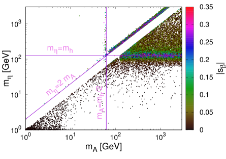
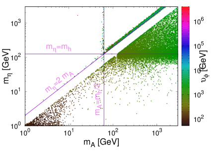
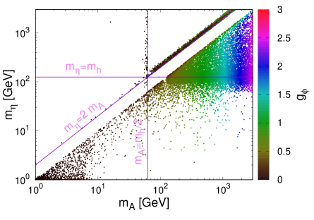
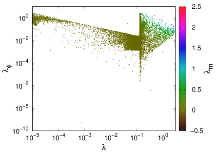
Figure 4: The new scalar mass $m_{\eta}$ versus the DM mass $m_{A}$, where the palette shows the scalar mixing (top-left), the new scalar vev (top-right) and the new gauge coupling (Bottom-left). Bottom-right: The quartic coupling $\lambda_{\phi}$ versus $\lambda$, where the coupling $\lambda_{m}$ is shown in the palette. All the above mentioned constraints in section III are taken into account during the scan over the parameters space.

In the top-left, top-right and bottom-left of Fig. 4, we show the viable $m_{\eta}-m_{A}$ space parameters, respecting the aforementioned constraints in the ranges listed in (37), where the palettes show the scalar mixing (top-left), the new scalar vev $\upsilon_{\phi}$ (top-right); and the new gauge coupling $g_{\phi}$ (bottom-left). One notices the existence of three distinct sub-regions in the $m_{\eta}-m_{A}$ plan, corresponding to (1) $m_{\eta}<m_{A}$, and it is the largest sub-region, (2) $m_{\eta}\gtrsim 2m_{A}$, and (3) $m_{A}\lesssim m_{h}/2$. Moreover, we remark that the constraints imposed on the parameters space can be easily evaded for values of $m_{\eta}$ and $m_{A}$ close to or larger than the electorweak scale, mostly in the top-right region in each plot, for the preferred ranges of the other parameters given as $\mid s_{\beta}\mid\lesssim 0.1$, $\upsilon_{\phi}\gtrsim 10^{3}$ and large values of $g_{\phi}\gtrsim 0.1$. One has to mention that most of the non-viable parameters space (empty regions in Fig. 4-top-right for example) are excluded mainly by DM direct detection and relic density requirements.

Recall that in setup, the new physics contribution to the oblique parameters $\Delta S$ and $\Delta T$ has negligible effect. As a consequence, having small values of $s_{\beta}$ (within the condition (41)) allows to have values $m_{\eta}$ close to or larger than the electorweak scale without violating the constraints imposed on $\Delta S$ and $\Delta T$. On the other hand, DM direct detection constraints given in (24), can be respected for large values of DM masses. Concerning the DM mass, that is given $m_{A}=g_{\phi}\upsilon_{\phi}/2$, having a small values of $g_{\phi}$ can be compensated by large values $\upsilon_{\phi}$ to get the desired values of $m_{A}$ that explain the parameters space in Fig. 4. One remarks that the scalar mixing is almost suppressed except in the regions around the degeneracies that are defined by the stright lines in Fig. 4, i.e., $m_{\eta}\gtrsim 2m_{A}$, $m_{A}\lesssim m_{h}/2$ and $m_{\eta}\thicksim m_{h}$.

In Fig. 4 bottom-right, we show the quartic coupling $\lambda_{\phi}$ versus $\lambda$ for the values of the coupling $\lambda_{m}$ shown in the palette. One notes that the constraints can be escaped when the mixing coupling $\lambda_{m}$ is small, preferably less than $0.5$, and the other quartic couplings $\lambda_{\phi}$ and $\lambda$ have values approximately greater than $10^{-3}$. This result is a consequence of applying the unitarity constraints given by the last inequality in (18). Clearly, large values of both $\lambda_{\phi}$ and $\lambda$ should be accompanied by small values of $\lambda_{m}$ to satisfy the unitarity constraints.

In Fig. 5, we show the signal strength (39) versus the total decay width of the new scalar ($\Gamma_{\eta}$ ) where the palettes show the ranges of $m_{\beta}$ and $\Gamma_{\eta}/m_{\eta}$ respectively.

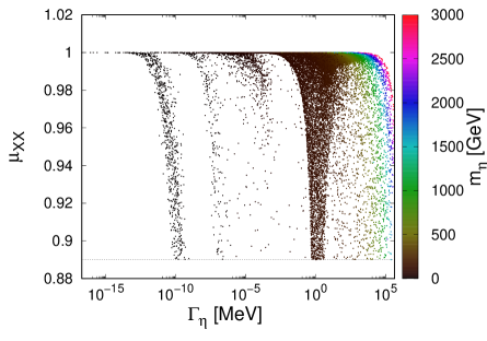
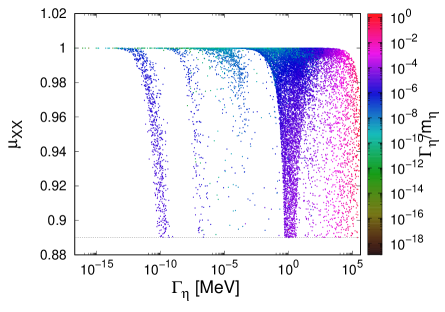
Figure 5: The signal strength (39) versus the total decay width of the new scalar ($\Gamma_{\eta}$ ). The palette shows the scalar mass ($m_{\eta}$ in GeV) mixing in left and the ratio $\Gamma_{\eta}/m_{\eta}$ in right side.

From (40), the signal strength has the value $c_{\beta}^{2}$ if the Higgs decaies only to SM particles, i.e., $\mathcal{B}_{BSM}=0$, which makes small mixing values the prefered ones as shown in Fig. 5-left. From Fig. 5-right, one notices that for $m_{\eta}\gtrsim 30\,GeV$, the total decay width has values $\Gamma_{\eta}\gtrsim 1\,MeV$, and it gets larger with large $m_{\eta}$ values. In Fig. 6, we show the DM-nucleon direct detection cross section (24) versus the DM mass (left) and the relative contribution of each annihilation channel to the total annhilation cross section at the freeze–out temperature (right).

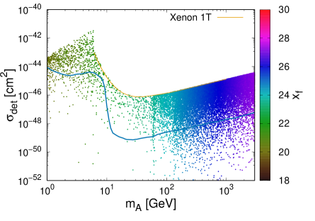
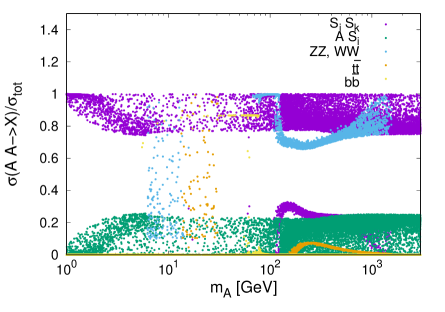
Figure 6: Left: the DM direct detection cros section versus the DM mass, where the palette shows the freeze-out parameter $x_{f}=m_{A}/T_{f}$. The orange line represents the recent Xenon-1T bound Aprile:2015uzo , and the blue one represents the neutrino floor Billard:2013qya . Right: the relative contributions to the thermal averaged cross section of different annihilation channels.

From Fig. 6-left, one remarks that viable dark vector DM scenario is possible at all DM masses range, and future experiements such as $Xenon-\,nT$ Aprile:2015uzo , can probe a significant part of the parameters space. Indeed, some of the benchmark points can not be probed since they are below the neutrino floor. The freeze-out parameter $x_{f}=m_{A}/T_{f}$, that is shown in the palette reads typical values $x_{f}\sim 17-28$. In order to figure out which the DM annhiliation channels is (are) effiecient, we present in Fig. 6-right the relative contribution of each DM annihilation channel ($f\bar{f}$, $WW$, $ZZ$, $hh$, $\eta\eta$ and $h\eta$) to the total thermally averaged annihilation cross section at the freeze-out temperature $T_{f}=m_{A}/x_{f}$ versus the DM mass.

Clearly from the Fig. 6-right, one notes that the cross section tends to be dominated by the annihilation into scalar channels ($hh$, $\eta\eta$ and $h\eta$) which are mediated by the of exchanging $h$, $\eta$ and $A_{i}$ bosons for all values of the DM mass. In addition the co-anihilation contribution (i.e., the second term in (30)) could be large as $20\%$ of the total thermally averaged annihilation cross section. The fact that the scalar channels $\eta\eta$ is also dominant for light DM ($\mathcal{O}(GeV)$) means that light DM implies light new scalr $\eta$. One has to mention aslo that the annihilation into gauge bosons could be efficient for DM masses around the $Z$ mass ($m_{Z}$) and also around $TeV$.

In Fig. 7, we present some branching ratios of the Higgs (left), and the main branching ratios of the scalar $\eta$ (right), especially $\gamma\gamma,A_{i}A_{i},hh,t\bar{t},b\bar{b},VV$ as functions of $\eta$ mass.

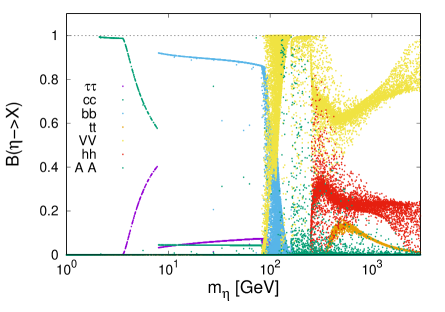
Figure 7: Left: the Higgs branching ratios. Right: the branching ratios of the new scalar decay versus its mass.

One notices from Fig. 7-left, that the branching ratios of $h\to gg$, $h\to\gamma\gamma$ and $h\to\gamma Z$ have values close the SM ones. Concerning the invisible and undetermined barnching ratios ($h\to AA$ and $h\to\eta\eta$), they can be significant withing the allowed range for some of the parameters space. From Fig. 7-right, one can learn that scalar $\eta$ decay can be dominated by a specific contribution for some $m_{\eta}$ intervals. For instance, the decay into light quarks, mainly $\eta\rightarrow c\bar{c}$, dominates for the mass window $m_{\eta}\apprle 8\,GeV$, while, it is dominated by $\eta\rightarrow b\bar{b}$ for $8\,GeV\apprle m_{\eta}\apprle 80\,GeV$. For the mass window $80\,GeV\apprle m_{\eta}\apprle 350\,GeV$ the decay will be dominated by $\eta\rightarrow WW,ZZ$ as well for some benchmark points with large scalar mass $m_{\eta}>2.5\,TeV$. The branching ratios of $\eta\rightarrow hh$ adn $\eta\rightarrow t\bar{t}$ have maximal values of $0.35$ and $0.18$, respectivley for scalar masses larger than $400\,GeV$. However, the invisible channel $\eta\rightarrow AA$ could be important for few benchmark points with mass betwenn $100\,GeV$ and $350\,GeV$.

By running the RGE in (25) up to the high energy scales $\Lambda=100\,TeV,\,10^{4}\,TeV$ and $\Lambda=m_{Planck}$, we obtain the running diemensionless scalar couplings. By imposing the conditions of perturbativity, vacuum stability and unitarity at these energy scales, the parameters space get reduced as shown in Fig. 8, where the plots top-left and bottom-right in Fig. 4, are obtained after after considering the above mentioned conditions.

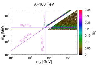
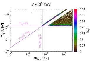
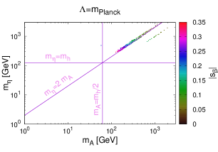
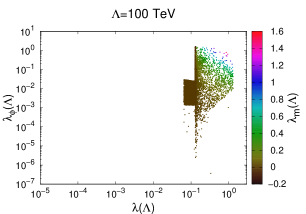
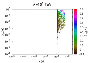
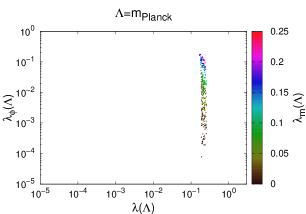
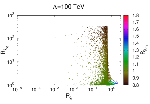
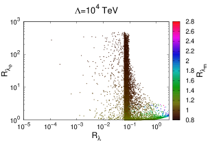
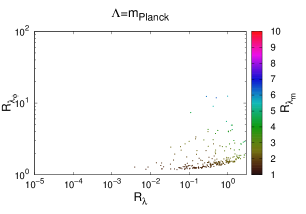
Figure 8: Up: the updated version of Fig. 4-top-left after considering the abovementioned conditions at scales $\Lambda=100~{}TeV$ (left), $\Lambda=10^{4}~{}TeV$ (middle) and $\Lambda=m_{Planck}$ (right). Middle: the updated version of Fig. 4-bottom-right within similar assumptions. Bottom: we show the coupling values at the runnuing scale, and in the bottom ones, we show their relativle enhancement $R_{\lambda_{i}}(\Lambda)=\lambda_{i}(\Lambda)/\lambda_{i}(m_{Z})$.

At higher scales, only benchmarks with non-suppressed $\lambda$ fulfills the above-mentioned conditions. In addition, only benchmarks points with positive $\lambda_{m}$ are favored. The enhancement in $\lambda_{\phi}$ could be two orders of magnitude lragere, which allows benchmark points with small $\lambda_{\phi}$ values. For intance, for 20k bencmark points shown in Fig. 4, the conditions of perturbativity, vacuum stability and unitarity at the scales $\Lambda=100\,TeV,\,10^{4}\,TeV$ and $\Lambda=m_{Planck}$, are filfilled only for $16700$, $11900$ and $260$, respectively.

V.2 Triple Higgs Coupling

In the SM, electroweak symmetry breaking relies on the parameters in the Higgs scalar potential, namely on the choice $\mu^{2}<0$ and $\lambda>0$. Hence, the partial experimental reconstruction of the Higgs scalar potential through measuring the triple Higgs coupling, $\lambda_{hhh}$, turns to be crucial to verify that the symmetry breaking is due to a SM-like Higgs sector Dolan:2012rv . Not only this, but it can also shed light on new physics Efrati:2014uta knowing that in many extensions of the SM, $\lambda_{hhh}$ can be modified by Higgs mixing effects or higher order corrections induced by new particles as we will show below. Consequently, the measurement of $\lambda_{hhh}$ is a crucial task in the LHC, although being challenging  Baglio:2012np ; Dolan:2012rv , and future collider experiments.

Indirect probe of the triple Higgs coupling can be carried out through investigating the loop effects in some observables such as the single Higgs production McCullough:2013rea ; Gorbahn:2016uoy ; Maltoni:2017ims , and the electroweak precision observables Kribs:2017znd . Using the 80 fb^-1 of LHC Run-2 data, and upon the assumption that new physics can affect only $\lambda_{hhh}$, ATLAS collaboration set recently the bound $-1.5<\lambda_{hhh}/\lambda_{hhh}^{SM}<6.7$ at $95\%$ CL ATLAS:2021jki . It should be noted that, direct measurement of the triple Higgs coupling at the LHC is possible and can be achieved through the di-Higgs production. This production is dominated by the gluon-gluon fusion process. In the SM, the production has two main contributions originating from the triangle diagram induced by the triple Higgs coupling, and from the box diagram with the top quark running in the loop. As noted in Chen:2019fhs , the two amplitudes, corresponding to the two contributions, interfere destructively. Consequently, at next-to-next-to-next-to-leading order (N³LO) and after including finite top quark mass effects, the estimated cross section at $14\,TeV$ LHC turn to be small and equal to $38.65\,fb$ Chen:2019fhs .

The analysis of the potential of measuring the di-Higgs production in the decay channels $b\bar{b}b\bar{b}$, $b\bar{b}\tau^{+}\tau^{-}$, $b\bar{b}WW^{*}$, $\gamma\gamma b\bar{b}$, $\gamma\gamma WW^{*}$ and $WW^{*}WW^{*}$, has been carried out in Refs. Dolan:2012rv ; Baglio:2012np ; Barr:2013tda ; Li:2013flc ; Cao:2015oaa ; Li:2015yia ; Cao:2015oxx ; Cao:2016zob ; He:2015spf ; Huang:2017jws ; Lu:2015jza ; Chang:2018uwu ; Papaefstathiou:2012qe ; Kim:2018cxf ; Buchalla:2018yce ; Kim:2019wns ; Li:2019uyy . At $13\,TeV$ LHC with the luminosity of $36.1\,fb^{-1}$, the combination of the six analyses results in the constraint $-5<\lambda_{hhh}/\lambda_{hhh}^{SM}<12$ at $95\%$ CL Abdughani:2020xfo . It is expected that, the sensitivity will be highly improved at the high-luminosity upgrade of the LHC (HL-LHC) Cepeda:2019klc and future hadron colliders Contino:2016spe . For instances, the future circular hadron collider, FCC-$hh$, with a center-of-mass energy of $100\,TeV$ and an integrated luminosity of $30\,ab^{-1}$ of data will allow reaching a $5\%$ accuracy (at $68\%$ CL) on the measurement of the triple Higgs coupling Goncalves:2018qas ; Chang:2018uwu ; Cepeda:2019klc .

The initial phase of the International Linear Collider (ILC) with a center-of-mass energy of $\sqrt{s}=$ $250\,GeV$ cannot directly probe $\lambda_{hhh}$ via di-Higgs production Fujii:2017vwa . However, this is not the case regarding single-Higgs production where an analysis using $2\,ab^{-1}$ of data can allow a measurement to $49\,\%$ accuracy, at $68\,\%$ CL deBlas:2019rxi . Higher precision of $27\,\%$ or $10\,\%$ , at $68\,\%$ CL, could possibly be reached using the data from ILC extensions to $500\,GeV$ ($4\,ab^{-1}$) or $1\,TeV$ ($8\,ab^{-1}$) respectively Fujii:2015jha ; Braathen:2019zoh . Moreover, at the same value of the confidence level, a more higher accuracy of $0.93<\lambda_{hhh}/\lambda_{hhh}^{SM}<1.11$ is possible to be reached using the combination of $1\,ab^{-1}$ of data at $380\,GeV$, $2.5\,ab^{-1}$ at $1.5\,TeV$, and $5\,ab^{-1}$ at $3\,TeV$ expected to be collected in the CLIC project Abramowicz:2016zbo ; Charles:2018vfv ; Roloff:2019crr ; Braathen:2019zoh .

In our model, the triple Higgs coupling $\lambda_{hhh}$ gets modified due to the mixing with the scalar $\eta$, and in addition, it receives new one-loop contributions by the scalar $\eta$ and the new gauge bosons $A_{i}$. Taking these contributions into account, we can parameterize $\lambda_{hhh}$ as

$$\lambda_{hhh}=\lambda_{hhh}^{SM}(1+\Delta_{hhh}),$$ (42)

where the one-loop triple Higgs coupling in the SM is given by Kanemura:2002vm ; Kanemura:2004mg

$$\lambda_{hhh}^{SM}\simeq\frac{3m_{h}^{2}}{\upsilon}\left[1-\frac{m_{t}^{4}}{\pi^{2}\upsilon^{2}m_{h}^{2}}\right].$$ (43)

According to the ILC physics group, the triple Higgs coupling can be measured at $\sqrt{s}=500\,GeV$ within the integrated luminosity $\mathcal{L}=500\,fb^{-1}$ with an accuracy less or equal to $20\,\%$ Fujii:2015jha . This implies that for the parameters space where $m_{\eta}\gg m_{h}$ , our model can tested at future linear colliders. Here, we estiamte the parameter $\Delta_{hhh}$ following Ahriche:2013vqa , where the Higgs trilinear self-coupling can be considered as the third derivative of the Higgs one-loop effective potential

$$\lambda_{hhh}=\frac{\partial^{3}V_{eff}}{\partial h^{3}},$$ (44)

where, the zero temperature one-loop effective potential $V_{eff}(h^{\prime},\eta^{\prime})$ is described in Appendix A. Therefore, one writes

$$\begin{array}[]{c}\lambda_{hhh}=\left.c_{\beta}^{3}\,\frac{\partial^{3}V_{eff}}{\partial h^{\prime 3}}-3c_{\beta}^{2}\,s_{\beta}\,\frac{\partial^{3}V_{eff}}{\partial\eta^{\prime}\partial h^{\prime 2}}+3c_{\beta}\,s_{\beta}^{2}\,\frac{\partial^{3}V_{eff}}{\partial\eta^{\prime 2}\partial h^{\prime}}-s_{\beta}^{3}\frac{\partial^{3}V_{eff}}{\partial\eta^{\prime 3}}\right|_{h^{\prime}=\eta^{\prime}=0}.\end{array}$$ (45)

At tree-level, these scalar triple couplings correspond to the $\rho_{h}$ parameter given in (15). For the bemchmarks points used previously, we show the Higgs triple coupling relative enhancement in Fig. 9.

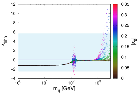
Figure 9: The triple Higgs relative enhancement $\Delta_{hhh}$ versus the new scalar mass, where the palette shows the scalar mixing. The skyblue band represents the allowed values of $\Delta_{hhh}$ by the recent ATLAS measurments ATLAS:2021jki .

The effect of these extra contributions can be either constructive or destructive according to the $\eta$ mass range. For instance, from Fig. 11, one notices that for scalar mass $m_{\eta}<m_{h}$ the coupling (44) is almsot supressed. While for the degenerate case $m_{\eta}\sim m_{h}$, we could have either enhancment or suppression. For $\eta$ mass larger than $1.2\,TeV$, some benchgmark points are already supressed by the ATLAS recent measurments ATLAS:2021jki .

V.3 The Di-Higgs Production

The di-Higgs production is not only interesting as its measurement allows to determine the trilinear Higgs couplings but also to describe the EWSB, i.e., it occurs via one Higgs or more. The triple Higgs coupling can be measured directly in di-Higgs boson production at $ILC$ through double Higgs-strahlung off $W$ or $Z$ bosons Gounaris:1979px ; Barger:1988jk ; Ilyin:1995iy ; Djouadi:1999gv ; Tian:2010np , $WW$ or $ZZ$ fusion Ilyin:1995iy ; Djouadi:1999gv ; Tian:2010np ; Boudjema:1995cb ; Barger:1988kb ; Dobrovolskaya:1990kx ; Abbasabadi:1988ja , also through gluon-gluon fusion in $pp$ colisions at the LHC Glover:1987nx ; Plehn:1996wb ; Dawson:1998py . The Higgs pair production processes in this model can be achieved three via Feynman diagrams as shown in Fig. 10. Indeed, there are two triangle diagrams mediated by the Higgs field $h$ and the new singlet scalar field $\eta$ instead of one diagram in the SM.

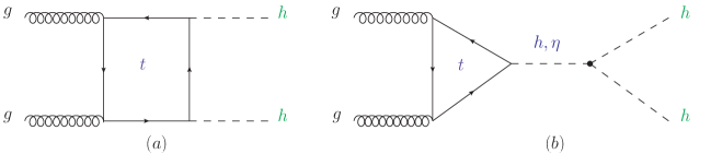
Figure 10: Feynman diagrams that contribute to the di-Higgs production via gluon fusion. The left (right) diagram is referred to be the box (triangle) in the literature.

In the SM, the di-Higgs production cross section has three contributions

$$\sigma^{SM}\left(hh\right)=\sigma_{\Square}+\sigma_{\triangle}+\sigma_{\triangle\Square},$$ (46)

which correspond to the box ($\sigma_{\Square}=70.1\,fb$), triangle ($\sigma_{\triangle}=9.66\,fb$); and interference ($\sigma_{\triangle\Square}=-49.9\,fb$), respectively Spira:1995mt . In this model, the di-Higgs production cross section can be written as

$$\sigma\left(hh\right)=\xi_{1}\sigma_{\Square}+\xi_{2}\sigma_{\triangle}+\xi_{3}\sigma_{\triangle\Square},$$ (47)

where the SM corresponds to $s_{\beta}=0$, i.e., $\xi_{1}=\xi_{2}=\xi_{3}=1$. The coeffetions $\xi_{i}$ in our model are modified with respect to the SM as

$$\xi_{1}=c_{\beta}^{4},\,\xi_{2} =\left(c_{\beta}\frac{\rho_{h}}{\lambda_{hhh}^{SM}}+s_{\beta}\frac{\rho_{2}}{\lambda_{hhh}^{SM}}\frac{s-m_{h}^{2}}{s-m_{\eta}^{2}}\right)^{2},\,\xi_{3}=c_{\beta}^{2}\left(c_{\beta}\frac{\rho_{h}}{\lambda_{hhh}^{SM}}+s_{\beta}\frac{\rho_{2}}{\lambda_{hhh}^{SM}}\frac{s-m_{h}^{2}}{s-m_{\eta}^{2}}\right),$$ (48)

with $\rho_{h}$ and $\rho_{2}$ are defined in (15), $\lambda_{hhh}^{SM}$ the Higgs triple coupling in the SM is given in (43); and $\sqrt{s}$ is the CM collision energy, which we will consider to be $\sqrt{s}=14\,\mathrm{TeV}$. In Fig. 11-left, we show the di-Higgs production cross section (47) at LHC14 scaled by its SM value versus the new scalar mass $m_{\eta}$ and the scalar mixing (in the palette), and in Fig. 11-right, we present the parameters $\xi$’s (48) for the benchmark points used previously.

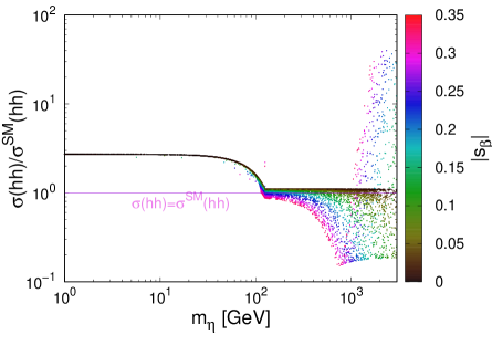
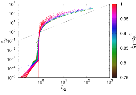
Figure 11: Left: the di-Higgs production cross section at $14\,TeV$, scaled by the SM value, where the palette shows the scalar mixing. Right: the parameters $\xi$’s (48) for the benchmark points used previously. The dashed line represent $\xi_{2}=\xi_{3}$, above which the destructive intereference contirubtion in (47) is larger, and hence the total crosss section is reduced.

Clearly for lighter new scalar $m_{\eta}<m_{h}$ the di-Higgs cross section masses is larger than the SM values by around 180 %, while, for heavier $\eta$ scalar $m_{\eta}>m_{h}$, it lies beween -92 % and 3000 %. Indeed, not all of the benchmark points would be in agreement with current data. In order to understand these results, Fig. 11-right shows the relation beween the patameters $\xi_{2}$ and $\xi_{3}$, where $\xi_{1}$ is shown in the palette. Since the interference term in (47) is negative, then the benchmark points above the straight line $\xi_{2}=\xi_{3}$ in Fig. 11-right correspond to larger cross section values. For lighter $\eta$ scalar $m_{\eta}<m_{h}/2$, where the undetermined Higgs decay channel $h\rightarrow\eta\eta$ is open, more negative searches can be used to constrain the parameters space, especially via the signatures $h\rightarrow\eta\eta\rightarrow bb\mu\mu$ ATLAS:2021ypo , $h\rightarrow\eta\eta\rightarrow 4b$ Aad:2020rtv ; and $h\rightarrow\eta\eta\rightarrow\gamma\gamma jj$ Aaboud:2018gmx . This analysis is postponed for a future work next .

VI Conclusion

In this work, we have considered an extension of the SM by enlarging the SM gauge symmetry by a non-abelian gauge group $SU(2)_{HS}$. In this case, the scalar sector of the model contains an extra new Higgs doublet that is required to spontaneously break the $SU(2)_{HS}$ gauge symmetry. The mixing of the extra doublet with the SM Higgs results, in the mass eigenstates basis, in two scalars denoted by $h$ and $\eta$. In our analysis, we identified $h$ as the SM neutral Higgs-like boson and adopted its mass to be $125\,GeV$. An important feature of the model is that the new gauge bosons, $A_{i}^{\mu}$ with i=1,2,3, associated with the group $SU(2)_{HS}$ are exactley degenerate in mass and can serve as vector DM candidates that interact with the SM through the Higgs portal.

To investigate such a possibility for DM candidate, we first considered all relevant constraints on the model, which include both theoretical and experimental ones, such as perturbative unitarity, vacuum stability, perturbativity, experimental bound on the DM direct detection, the observed DM relic density, the constraints from the Higgs decay where the invisible or/and undetermined branching ratio where the Higgs total decay width must respect the existing experimental constraints. As a result, we showed that it is possible to have viable parameters space in which the masses of the DM candidates lies from few GeV to the TeV scale, which is still within the reach of high energy collider experiments. Regarding the limits from direct detection DM experiements, it is easily acomodated in this model for most of the values of DM and new scalar masses. In adition, the observed relic density values can be achieved by many anihilation channels acording to the DM mass, and on top of that, the co-anihilation ($A_{i}A_{j}\rightarrow hA_{k}$) effcect could be importan as it may reach 25 % of the total thermally averaged anihilation cross section.

In our wrok, we considered the conditions of perturbativity, vacuum stabilty and perturbative unitarity, but these conditions may not be fulfilled at higher scales. By runing the quartic scalar and gauge couplings at higher scale $\Lambda$ using the RGE (25), we found that 16.5 %, 40 % and 98.7 % of the benchmark points will be ruled out due these conditions at scale values $\Lambda=100\,TeV,\,10^{4}\,TeV,\,m_{Planck}$, respectively.

In the decoupling limit $m_{\eta}>>m_{h}$, as in many extensions of the SM, the Higgs mixing effects and the presence of new fields coupled to the Higgs doublet induces significant corrections to the SM prediction of the triple Higgs self-couplings $\lambda_{hhh}=(1+\Delta_{hhh})\lambda_{hhh}^{SM}$. We have found that, up to one-loop level, the effect of the new scalar $\eta$ and the vector DM $A_{i}$ leads to a relative enhancement ($\Delta_{hhh}$) that lies between -250 % and +1200 %. Indeed, part of these benchamrk points are already esxcluded by the recent measerments by ATLAS ATLAS:2021jki . However, in the case $m_{\eta}<m_{h}$, the cross the di-Higgs gets enhanced by around 180 %, which makes the signatures $h\rightarrow\eta\eta\rightarrow bb\mu\mu$, $h\rightarrow\eta\eta\rightarrow 4b$ and $h\rightarrow\eta\eta\rightarrow\gamma\gamma jj$ very useful to put more constraints on the model free parameters.

Appendix A The One-Loop Effective Potential

The zero temperature one-loop effective potential can be given in the $\overline{DR}$ scheme by

$$V_{eff}\left(h^{\prime},\eta^{\prime}\right) =V^{0}\left(h^{\prime},\eta^{\prime}\right)+\frac{1}{64\pi^{2}}\sum_{i}n_{i}m_{i}^{4}\left(h^{\prime},\eta^{\prime}\right)\left(\log\left(\frac{m_{i}^{2}\left(h^{\prime},\eta^{\prime}\right)}{\Lambda^{2}}\right)-\frac{3}{2}\right),$$

where, $V^{0}\left(h^{\prime},\eta^{\prime}\right)$ is the tree-level potential, $n_{i}$ is the number of internal degrees of freedom of the $i\,$th particle ($n_{h}=n_{\eta}=1$, $n_{Z}=3$, $n_{W}=6$, $n_{t}=-12$ and $n_{A_{i}}=9$). Here, $m_{i}^{2}\left(h^{\prime},\eta^{\prime}\right)$ are the field-dependent squared masses; and $\Lambda$ is the renormalization scale, which we will choose to be the Higgs mass $\Lambda=125.18\,\mathrm{GeV}$.

The field-dependent squared masses $m_{i}(h^{\prime},\eta^{\prime})$ of all the contributing particles, so we have the field-dependent masses of the Goldstone bosons $\chi$ and $\xi$

$$m_{\chi}^{2}=\mu^{2}+\lambda h^{\prime 2}+\frac{\lambda_{m}}{2}\eta^{\prime 2},\,m_{\xi}^{2}=\mu_{\phi}^{2}+\lambda_{\phi}\eta^{\prime 2}+\frac{\lambda_{m}}{2}h^{\prime 2}.$$ (49)

The field-dependent masses of the electroweak gauge bosons and top quark are given in the symmetric phase (i.e., for $<h>=<\phi>=0$) by

$$m_{t}^{2}=\frac{y_{t}^{2}}{2}h^{\prime 2},\,m_{W}^{2}=\frac{g_{2}^{2}}{4}h^{\prime 2},\,m_{W^{3}}^{2}=\frac{g_{2}^{2}}{4}h^{\prime 2},\,m_{W^{3}-B}^{2}=\frac{g_{1}^{2}}{4}h^{\prime 2},m_{B}^{2}=\frac{g_{1}^{2}}{4}h^{\prime 2},\,m_{A}^{2}=\frac{g_{\phi}^{2}}{4}\eta^{\prime 2},$$ (50)

where the diagonalization of the {$W^{3}-B$} matrix gives $m_{\gamma}=0$ and $m_{Z}^{2}=\frac{\left(g_{1}^{2}+g_{2}^{2}\right)}{4}h^{\prime 2}$. Here, $y_{t}$ denotes the top-quark Yukawa coupling, and $g_{1}$, $g_{2}$ and $g_{\phi}$ are the gauge couplings of $U(1)_{Y}$, $SU(2)_{L}$ and $SU(2)_{HS}$, respectively.

For the field-dependent masses of $h$ and $\eta$ can be obtained as the eigensvalues of the squared mass matrice in the basis $\left\{h^{\prime},\eta^{\prime}\right\}$, which is given by

$$M^{2}=\left(\begin{array}[]{cc}A&C\\ C&B\end{array}\right),$$ (51)

with $A=\mu^{2}+3\lambda h^{\prime 2}+\frac{\lambda_{m}}{2}\eta^{\prime 2},\,B=\mu_{\phi}^{2}+3\lambda_{\phi}\eta^{\prime 2}+\frac{\lambda_{m}}{2}h^{\prime 2},\,C=\lambda_{m}h^{\prime}\eta^{\prime}$. Then, the field dependant eigenmasses are given by $m_{h,\eta}^{2}\left(h^{\prime},\eta^{\prime}\right)=\frac{1}{2}\left(A+B\mp\sqrt{(A-B)^{2}+C^{2}}\right)$.

Appendix B The Cross Section for $hh$, $\eta\eta$, $h\eta$, $Ah$ & $A\eta$

Here, we give the formulas of the parameters used in the cross section of the final states $hh$, $\eta\eta$, $h\eta$, $Ah$ & $A\eta$ given in (34), (36) and (35). We denote by $H$ either $h$ or $\eta$, so the parameters are given by

$$A =\frac{2m_{H}^{2}-s}{2m_{A}^{2}},\,B=\frac{s}{2m_{A}^{2}}\sqrt{\left(1-\frac{4m_{H}^{2}}{s}\right)\left(1-\frac{4m_{A}^{2}}{s}\right)},\,Q_{0}=\frac{\sqrt{1-\frac{4m_{H}^{2}}{s}}}{16\pi},$$

$$Q_{1} =\frac{2q^{4}}{9\upsilon_{\phi}^{4}m_{A}^{4}}(48m_{A}^{8}-32m_{A}^{6}m_{H}^{2}+24m_{A}^{4}m_{H}^{4}-16m_{A}^{4}m_{H}^{2}s+4m_{A}^{4}s^{2}-8m_{A}^{2}m_{H}^{6}+4m_{A}^{2}m_{H}^{4}s+m_{H}^{8}),$$

$$Q_{2} =\frac{4q^{4}}{9\upsilon_{\phi}^{4}m_{A}^{2}\left(s-2m_{H}^{2}\right)}(-48m_{A}^{8}+32m_{A}^{6}m_{H}^{2}-8m_{A}^{4}m_{H}^{4}+4m_{A}^{4}s^{2}-8m_{A}^{2}m_{H}^{6}+4m_{A}^{2}m_{H}^{2}s^{2}-2m_{A}^{2}s^{3}$$

$$+3m_{H}^{8}-m_{H}^{4}s^{2})+\frac{4q^{2}\Re(R)}{9\upsilon_{\phi}^{4}m_{A}^{2}\left(s-2m_{H}^{2}\right)}(-48m_{A}^{6}m_{H}^{2}+24m_{A}^{6}s+16m_{A}^{4}m_{H}^{4}-4m_{A}^{4}s^{2}-4m_{A}^{2}m_{H}^{6}$$

$$+10m_{A}^{2}m_{H}^{4}s-8m_{A}^{2}m_{H}^{2}s^{2}+2m_{A}^{2}s^{3}-2m_{H}^{6}s+m_{H}^{4}s^{2}),$$

$$Q_{3} =\frac{4q^{4}}{9\upsilon_{\phi}^{4}}(-4m_{A}^{4}+4m_{A}^{2}m_{H}^{2}-6m_{A}^{2}s+m_{H}^{4}+2m_{H}^{2}s)+\frac{8q^{2}\Re(R)}{9\upsilon_{\phi}^{4}}(-4m_{A}^{2}m_{H}^{2}+4m_{A}^{2}s-m_{H}^{2}s)$$

$$+\frac{\left|R\right|^{2}}{9\upsilon_{\phi}^{4}}(12m_{A}^{4}-4m_{A}^{2}s+s^{2}),$$

$$Q_{4} =\frac{4m_{A}^{2}q^{4}}{9\upsilon_{\phi}^{4}\left(2m_{H}^{2}-s\right)}(8m_{A}^{4}-8m_{A}^{2}m_{H}^{2}+8m_{A}^{2}s+2m_{H}^{4}-4m_{H}^{2}+s^{2})+\frac{4m_{A}^{2}q^{2}\Re(R)}{9\upsilon_{\phi}^{4}\left(2m_{H}^{2}-s\right)}(4m_{A}^{2}m_{H}^{2}$$

$$-2m_{A}^{2}s+2m_{H}^{2}s-s^{2}),\,Q_{5}=-\frac{2q^{4}m_{A}^{4}}{3\upsilon_{\phi}^{4}},\,Q_{6}=\frac{4q^{4}m_{A}^{6}}{9\upsilon_{\phi}^{4}\left(2m_{H}^{2}-s\right)}.$$ (52)

with $\left\{q,R\right\}=\left\{s_{\beta},\frac{c_{\beta}\rho_{2}\upsilon_{\phi}}{s-m_{\eta}^{2}+im_{\eta}\Gamma_{\eta}}-\frac{s_{\beta}\rho_{h}\upsilon_{\phi}}{s-m_{h}^{2}+im_{h}\Gamma_{h}}+s_{\beta}^{2}\right\}$ for $h$; and $\left\{q,R\right\}=\left\{-c_{\beta},\frac{s_{\beta}\rho_{\eta}\upsilon_{\phi}}{s-m_{\eta}^{2}+im_{\eta}\Gamma_{\eta}}+\frac{c_{\beta}\rho_{1}\upsilon_{\phi}}{s-m_{h}^{2}+im_{h}\Gamma_{h}}+c_{\beta}^{2}\right\}$ for $\eta$, where $\Gamma_{h}$ ($\Gamma_{\eta}$) is the total decay width of the Higgs (scalar $\eta$).

For the final state $h\eta$, the parameters are given by

$$A =\frac{m_{h}^{2}+m_{\eta}^{2}-s}{2m_{A}^{2}},\,B=\frac{1}{2m_{A}^{2}}\sqrt{1-\frac{4m_{A}^{2}}{s}}\sqrt{(s-m_{h}^{2}-m_{\eta}^{2})^{2}-4m_{h}^{2}m_{\eta}^{2}},$$

$$Q_{0} =\frac{\sqrt{(s-m_{h}^{2}-m_{\eta}^{2})^{2}-4m_{h}^{2}m_{\eta}^{2}}}{16\pi\,s},\,R=-\frac{s_{\beta}\rho_{2}\upsilon_{\phi}}{s-m_{h}^{2}+im_{h}\Gamma_{h}}+\frac{c_{\beta}\rho_{1}\upsilon_{\phi}}{s-m_{\eta}^{2}+im_{\eta}\Gamma_{\eta}}-c_{\beta}s_{\beta},$$

$$Q_{1} =\frac{s_{2\beta}^{2}}{36m_{A}^{4}\upsilon_{\phi}^{4}}(48m_{A}^{8}-16m_{A}^{6}m_{\eta}^{2}-16m_{A}^{6}m_{h}^{2}+8m_{A}^{4}m_{\eta}^{4}+8m_{A}^{4}m_{\eta}^{2}m_{h}^{2}-8m_{A}^{4}m_{\eta}^{2}s+8m_{A}^{4}m_{h}^{4}-8m_{A}^{4}m_{h}^{2}s$$

$$+4m_{A}^{4}s^{2}-4m_{A}^{2}m_{\eta}^{4}m_{h}^{2}-4m_{A}^{2}m_{\eta}^{2}m_{h}^{4}+4m_{A}^{2}m_{\eta}^{2}m_{h}^{2}s+m_{\eta}^{4}m_{h}^{4}),$$

$$Q_{2} =\frac{s_{2\beta}^{2}}{18m_{A}^{2}\upsilon_{\phi}^{4}}(-4m_{A}^{4}m_{\eta}^{2}-4m_{A}^{4}m_{h}^{2}+8m_{A}^{4}s+8m_{A}^{2}m_{\eta}^{2}m_{h}^{2}-2m_{A}^{2}m_{\eta}^{2}s-2m_{A}^{2}m_{h}^{2}s-m_{\eta}^{4}m_{h}^{2}-m_{\eta}^{2}m_{h}^{4})$$

$$+\frac{\Re(R)s_{2\beta}}{9m_{A}^{2}\upsilon_{\phi}^{4}}(-24m_{A}^{6}+4m_{A}^{4}m_{\eta}^{2}+4m_{A}^{4}m_{h}^{2}+4m_{A}^{4}s-2m_{A}^{2}m_{\eta}^{4}+2m_{A}^{2}m_{\eta}^{2}m_{h}^{2}+2m_{A}^{2}m_{\eta}^{2}s-2m_{A}^{2}m_{h}^{4}$$

$$+2m_{A}^{2}m_{h}^{2}s-2m_{A}^{2}s^{2}-m_{\eta}^{2}m_{h}^{2}s),$$

$$Q_{3} =\frac{\left|R\right|^{2}}{9\upsilon_{\phi}^{4}}(12m_{A}^{4}-4m_{A}^{2}s+s^{2})+\frac{s_{2\beta}\Re(R)}{9\upsilon_{\phi}^{4}}(2m_{A}^{2}m_{\eta}^{2}+2m_{A}^{2}m_{h}^{2}-4m_{A}^{2}s+m_{\eta}^{2}s+m_{h}^{2}s)$$

$$+\frac{s_{2\beta}^{2}}{36\upsilon_{\phi}^{4}}(8m_{A}^{4}-4m_{A}^{2}m_{\eta}^{2}-4m_{A}^{2}m_{h}^{2}+4m_{A}^{2}s+4m_{\eta}^{2}m_{h}^{2}+m_{\eta}^{4}+m_{h}^{4}),$$

$$Q_{4} =-\frac{s_{2\beta}\Re(R)m_{A}^{2}}{9\upsilon_{\phi}^{4}}(2m_{A}^{2}+s)-\frac{s_{2\beta}^{2}m_{A}^{2}}{18\upsilon_{\phi}^{4}}(m_{\eta}^{2}+m_{h}^{2}),\,Q_{5}=\frac{s_{2\beta}^{2}}{36}\frac{m_{A}^{4}}{\upsilon_{\phi}^{4}},\,Q_{6}=0.$$ (53)

For the final states $Ah$ and $A\eta$, the parameters are given by

$$A =\frac{m_{A}^{2}+m_{H}^{2}-s}{2m_{A}^{2}},\,B=B=\frac{1}{2m_{A}^{2}}\sqrt{1-\frac{4m_{A}^{2}}{s}}\sqrt{(s-m_{H}^{2}-m_{A}^{2})^{2}-4m_{H}^{2}m_{A}^{2}},$$

$$Q_{0} =\frac{\sqrt{(s-m_{H}^{2}-m_{A}^{2})^{2}-4m_{H}^{2}m_{A}^{2}}}{16\pi\,s},$$

$$Q_{1} =-\frac{q^{2}}{36m_{A}^{4}\upsilon_{\phi}^{4}}(20m_{A}^{8}+588m_{A}^{6}m_{H}^{2}+256m_{A}^{6}s-461m_{A}^{4}m_{H}^{4}-352m_{A}^{4}m_{H}^{2}s-96m_{A}^{4}s^{2}$$

$$+72m_{A}^{2}m_{H}^{6}+108m_{A}^{2}m_{H}^{4}s+128m_{A}^{2}m_{H}^{2}s^{2}-36m_{H}^{4}s^{2}),$$

$$Q_{2} =-\frac{q^{2}}{18m_{A}^{2}\upsilon_{\phi}^{4}(s-m_{A}^{2})}(336m_{A}^{8}-165m_{A}^{6}m_{H}^{2}-264m_{A}^{6}s-37m_{A}^{4}m_{H}^{4}+241m_{A}^{4}m_{H}^{2}s$$

$$+128m_{A}^{4}s^{2}-21m_{A}^{2}m_{H}^{4}s-88m_{A}^{2}m_{H}^{2}s^{2}-32m_{A}^{2}s^{3}-18m_{H}^{4}s^{2}+36m_{H}^{2}s^{3}),$$

$$Q_{3} =\frac{q^{2}}{36\upsilon_{\phi}^{4}(s-m_{A}^{2})^{2}}(-591m_{A}^{8}+480m_{A}^{6}m_{H}^{2}-302m_{A}^{6}s+m_{A}^{4}m_{H}^{4}-416m_{A}^{4}m_{H}^{2}s$$

$$+189m_{A}^{4}s^{2}+6m_{A}^{2}m_{H}^{4}s+104m_{A}^{2}m_{H}^{2}s^{2}-100m_{A}^{2}s^{3}+9m_{H}^{4}s^{2}-72m_{H}^{2}s^{3}+36s^{4}),$$

$$Q_{4} =\frac{q^{2}m_{A}^{2}}{18\upsilon_{\phi}^{4}(s-m_{A}^{2})^{2}}(-153m_{A}^{6}-69m_{A}^{4}m_{H}^{2}+164m_{A}^{4}s-2m_{A}^{2}m_{H}^{2}s-29m_{A}^{2}s^{2}-9m_{H}^{2}s^{2}+18s^{3}),$$

$$Q_{5} =\frac{q^{2}m_{A}^{4}}{36\upsilon_{\phi}^{4}(s-m_{A}^{2})^{2}}(153m_{A}^{4}-2m_{A}^{2}s+9s^{2}),\,Q_{6}=0,$$ (54)

with $\{m_{H},q^{2}\}=\{m_{h},s_{\beta}\},\{m_{\eta},-c_{\beta}\}$ for the final states $Ah$ and $A\eta$, respectively.

References

- (1) F. Zwicky, Helv. Phys. Acta 6, 110 (1933) [Gen. Rel. Grav. 41, 207 (2009)]. E. Corbelli and P. Salucci, Mon. Not. Roy. Astron. Soc. 311, 441 (2000) [arXiv:astro-ph/9909252 [astro-ph]]. D. P. Roy, [arXiv:physics/0007025 [physics]].
- (2) N. Aghanim et al. [Planck], Astron. Astrophys. 641, A6 (2020) [arXiv:1807.06209 [astro-ph.CO]].
- (3) For example: N. G. Deshpande and E. Ma, Phys. Rev. D 18(1978), 2574 S. Hannestad, A. Mirizzi, G. G. Raffelt and Y. Y. Y. Wong, JCAP 04 (2008), 019 [arXiv:0803.1585 [astro-ph]]. T. Hambye and M. H. G. Tytgat, Phys. Lett. B 659, 651 (2008) [arXiv:0707.0633 [hep-ph]]. A. Ahriche and S. Nasri, Phys. Rev. D 85 (2012), 093007 [arXiv:1201.4614 [hep-ph]]. C. Gross, O. Lebedev and T. Toma, Phys. Rev. Lett. 119, no.19, 191801 (2017) [arXiv:1708.02253 [hep-ph]]. Y. Abe, T. Toma and K. Tsumura, JHEP 05(2020), 057 [arXiv:2001.03954 [hep-ph]]. N. Okada, D. Raut and Q. Shafi, [arXiv:2001.05910 [hep-ph]]. A. Ahmed, S. Najjari and C. B. Verhaaren, JHEP 06(2020), 007 [arXiv:2003.08947 [hep-ph]]. J. McDonald, Phys. Rev. D 50(1994), 3637 [arXiv:hep-ph/0702143 [hep-ph]]. J. McDonald, Phys. Rev. Lett. 88, 091304 (2002) [arXiv:hep-ph/0106249 [hep-ph]]. C. P. Burgess, M. Pospelov and T. ter Veldhuis, Nucl. Phys. B 619, 709 (2001) [arXiv:hep-ph/0011335 [hep-ph]]. C. Boehm and P. Fayet, Nucl. Phys. B 683, 219 (2004) [arXiv:hep-ph/0305261 [hep-ph]]. C. Boehm, Y. Farzan, T. Hambye, S. Palomares-Ruiz and S. Pascoli, Phys. Rev. D 77 (2008), 043516 [arXiv:hep-ph/0612228 [hep-ph]]. V. Barger, P. Langacker, M. McCaskey, M. J. Ramsey-Musolf and G. Shaughnessy, Phys. Rev. D 77 (2008), 035005 [arXiv:0706.4311 [hep-ph]]. S. Andreas, T. Hambye and M. H. G. Tytgat, JCAP 10 (2008), 034 [arXiv:0808.0255 [hep-ph]].
- (4) For example: P. Nath and R. L. Arnowitt, [arXiv:hep-ph/9610460 [hep-ph]]. N. Baouche and A. Ahriche, Phys. Rev. D 96 (2017), 055029 [arXiv:1707.05263 [hep-ph]]. L. Covi, L. Roszkowski, R. Ruiz de Austri and M. Small, JHEP 06(2004), 003 [arXiv:hep-ph/0402240 [hep-ph]]. M. Pospelov, A. Ritz and M. B. Voloshin, Phys. Lett. B 662, 53 (2008) [arXiv:0711.4866 [hep-ph]]. G. Belanger, A. Pukhov and G. Servant, JCAP 01(2008), 009 [arXiv:0706.0526 [hep-ph]]. L. Covi, M. Grefe, A. Ibarra and D. Tran, JCAP 01(2009), 029 [arXiv:0809.5030 [hep-ph]]. S. Ipek, D. McKeen and A. E. Nelson, Phys. Rev. D 90(2014), no.5, 055021 [arXiv:1404.3716 [hep-ph]]. K. Ghorbani, JCAP 01(2015), 015 [arXiv:1408.4929 [hep-ph]]. A. Ahriche and S. Nasri, JCAP 07 (2013), 035 [arXiv:1304.2055 [hep-ph]]. A. Ahriche, C. S. Chen, K. L. McDonald and S. Nasri, Phys. Rev. D 90 (2014), 015024 [arXiv:1404.2696 [hep-ph]]. A. Ahriche, K. L. McDonald and S. Nasri, JHEP 10 (2014), 167 [arXiv:1404.5917 [hep-ph]]. A. Ahriche, K. L. McDonald, S. Nasri and T. Toma, Phys. Lett. B 746 (2015), 430-435 [arXiv:1504.05755 [hep-ph]]. A. Ahriche, K. L. McDonald and S. Nasri, JHEP 02 (2016), 038 [arXiv:1508.02607 [hep-ph]]. A. Ahriche, K. L. McDonald, S. Nasri and I. Picek, Phys. Lett. B 757 (2016), 399-404 [arXiv:1603.01247 [hep-ph]]. A. Ahriche, A. Manning, K. L. McDonald and S. Nasri, Phys. Rev. D 94 (2016) no.5, 053005 [arXiv:1604.05995 [hep-ph]]. A. Ahriche, A. Jueid and S. Nasri, Phys. Rev. D 97 (2018) no.9, 095012 [arXiv:1710.03824 [hep-ph]]. A. Ahriche, A. Arhrib, A. Jueid, S. Nasri and A. de La Puente, Phys. Rev. D 101 (2020) no.3, 035038 [arXiv:1811.00490 [hep-ph]]. A. Ahriche, A. Jueid and S. Nasri, Phys. Lett. B 814 (2021), 136077 [arXiv:2007.05845 [hep-ph]]. S. Baek, P. Ko and J. Li, Phys. Rev. D 95(2017), no.7, 075011 [arXiv:1701.04131 [hep-ph]].
- (5) For example: H. C. Cheng, J. L. Feng and K. T. Matchev, Phys. Rev. Lett. 89, 211301 (2002) [arXiv:hep-ph/0207125 [hep-ph]]. D. Hooper and G. D. Kribs, Phys. Rev. D 70(2004), 115004 [arXiv:hep-ph/0406026 [hep-ph]]. H. C. Cheng and I. Low, JHEP 09(2003), 051 [arXiv:hep-ph/0308199 [hep-ph]]. A. Birkedal, A. Noble, M. Perelstein and A. Spray, Phys. Rev. D 74(2006), 035002 [arXiv:hep-ph/0603077 [hep-ph]]. S. Kanemura, S. Matsumoto, T. Nabeshima and N. Okada, Phys. Rev. D 82(2010), 055026 [arXiv:1005.5651 [hep-ph]]. O. Lebedev, H. M. Lee and Y. Mambrini, Phys. Lett. B 707, 570 (2012) [arXiv:1111.4482 [hep-ph]]. T. Abe, M. Kakizaki, S. Matsumoto and O. Seto, Phys. Lett. B 713, 211 (2012) [arXiv:1202.5902 [hep-ph]]. Y. Farzan and A. R. Akbarieh, JCAP 10(2012), 026 [arXiv:1207.4272 [hep-ph]]. J. M. Hyde, A. J. Long and T. Vachaspati, Phys. Rev. D 89(2014), 065031 [arXiv:1312.4573 [hep-ph]]. P. Ko, W. I. Park and Y. Tang, JCAP 09(2014), 013 [arXiv:1404.5257 [hep-ph]]. S. Baek, P. Ko, W. I. Park and E. Senaha, JHEP 05, 036 (2013) [arXiv:1212.2131 [hep-ph]]. S. Baek, P. Ko and W. I. Park, Phys. Rev. D 90(2014), no.5, 055014 [arXiv:1405.3530 [hep-ph]]. J. H. Yu, Phys. Rev. D 90(2014), no.9, 095010 [arXiv:1409.3227 [hep-ph]]. C. R. Chen, Y. K. Chu and H. C. Tsai, Phys. Lett. B 741, 205 (2015) [arXiv:1410.0918 [hep-ph]]. H. Zhang, C. S. Li, Q. H. Cao and Z. Li, Phys. Rev. D 82(2010), 075003 [arXiv:0910.2831 [hep-ph]]. J. L. Diaz-Cruz and E. Ma, Phys. Lett. B 695, 264 (2011) [arXiv:1007.2631 [hep-ph]]. S. Bhattacharya, J. L. Diaz-Cruz, E. Ma and D. Wegman, Phys. Rev. D 85(2012), 055008 [arXiv:1107.2093 [hep-ph]]. T. Hambye and A. Strumia, Phys. Rev. D 88(2013), 055022 [arXiv:1306.2329 [hep-ph]]. H. Davoudiasl and I. M. Lewis, Phys. Rev. D 89(2014), no.5, 055026 [arXiv:1309.6640 [hep-ph]]. S. Baek, P. Ko and W. I. Park, JCAP 10(2014), 067 [arXiv:1311.1035 [hep-ph]]. V. V. Khoze and G. Ro, JHEP 10(2014), 061 [arXiv:1406.2291 [hep-ph]]. S. Fraser, E. Ma and M. Zakeri, Int. J. Mod. Phys. A 30, no.03, 1550018 (2015) [arXiv:1409.1162 [hep-ph]]. A. Karam and K. Tamvakis, Phys. Rev. D 92(2015), no.7, 075010 [arXiv:1508.03031 [hep-ph]]. T. Abe, M. Fujiwara, J. Hisano and K. Matsushita, JHEP 07(2020), 136 [arXiv:2004.00884 [hep-ph]].
- (6) T. Hambye, JHEP 01(2009), 028 [arXiv:0811.0172 [hep-ph]].
- (7) G. Arcadi, A. Djouadi and M. Raidal, Phys. Rept. 842, 1 (2020) [arXiv:1903.03616 [hep-ph]].
- (8) J. M. Cornwall, D. N. Levin and G. Tiktopoulos, Phys. Rev. D 10(1974), 1145 [erratum: Phys. Rev. D 11(1975), 972] B. W. Lee, C. Quigg and H. B. Thacker, Phys. Rev. D 16(1977), 1519 B. W. Lee, C. Quigg and H. B. Thacker, Phys. Rev. Lett. 38, 883 (1977) S. Kanemura, T. Kubota and E. Takasugi, Phys. Lett. B 313, 155 (1993) [arXiv:hep-ph/9303263 [hep-ph]]. A. G. Akeroyd, A. Arhrib and E. M. Naimi, Phys. Lett. B 490, 119 (2000) [arXiv:hep-ph/0006035 [hep-ph]]. J. Horejsi and M. Kladiva, Eur. Phys. J. C 46, 81 (2006) [arXiv:hep-ph/0510154 [hep-ph]].
- (9) A. Arhrib, [arXiv:hep-ph/0012353 [hep-ph]].
- (10) G. Aad et al. [ATLAS], Phys. Rev. D 101(2020), no.1, 012002 [arXiv:1909.02845 [hep-ex]].
- (11) M. Aaboud et al. [ATLAS], Phys. Rev. Lett. 122 (2019) no.23, 231801 [arXiv:1904.05105 [hep-ex]].
- (12) [ATLAS], “Combination of searches for invisible Higgs boson decays with the ATLAS experiment,” ATLAS-CONF-2020-052.
- (13) A. M. Sirunyan et al. [CMS], Phys. Lett. B 793 (2019), 520-551 [arXiv:1809.05937 [hep-ex]].
- (14) V. Khachatryan et al. [CMS], Phys. Rev. D 92(2015), no.7, 072010 [arXiv:1507.06656 [hep-ex]].
- (15) M. Aaboud et al. [ATLAS], Phys. Lett. B 786, 223 (2018) [arXiv:1808.01191 [hep-ex]].
- (16) E. Aprile et al. [XENON], JCAP 04 (2016), 027 [arXiv:1512.07501 [physics.ins-det]].
- (17) A. Falkowski, C. Gross and O. Lebedev, JHEP 05(2015), 057 [arXiv:1502.01361 [hep-ph]].
- (18) M. Srednicki, R. Watkins and K. A. Olive, Nucl. Phys. B 310, 693 (1988) E. W. Kolb and M. S. Turner, Front. Phys. 69, 1 (1990)
- (19) G. Aad et al. [ATLAS and CMS], and 8 TeV,” JHEP 08(2016), 045 [arXiv:1606.02266 [hep-ex]].
- (20) A. M. Sirunyan et al. [CMS], Phys. Rev. Lett. 121, no.12, 121801 (2018) [arXiv:1808.08242 [hep-ex]].
- (21) M. Aaboud et al. [ATLAS], Phys. Lett. B 786, 59-86 (2018) [arXiv:1808.08238 [hep-ex]].
- (22) A. M. Sirunyan et al. [CMS], Eur. Phys. J. C 79, no.5, 421 (2019) [arXiv:1809.10733 [hep-ex]].
- (23) M. Cepeda, S. Gori, P. Ilten, M. Kado, F. Riva, R. Abdul Khalek, A. Aboubrahim, J. Alimena, S. Alioli and A. Alves, et al. CERN Yellow Rep. Monogr. 7, 221 (2019) [arXiv:1902.00134 [hep-ph]].
- (24) G. Arcadi, A. Djouadi and M. Kado, Phys. Lett. B 805 (2020), 135427 [arXiv:2001.10750 [hep-ph]].
- (25) J. Billard, L. Strigari and E. Figueroa-Feliciano, Phys. Rev. D 89 (2014) no.2, 023524 [arXiv:1307.5458 [hep-ph]].
- (26) M. J. Dolan, C. Englert and M. Spannowsky, JHEP 10, 112 (2012) [arXiv:1206.5001 [hep-ph]].
- (27) A. Efrati and Y. Nir, [arXiv:1401.0935 [hep-ph]].
- (28) J. Baglio, A. Djouadi, R. Gröber, M. M. MÌhlleitner, J. Quevillon and M. Spira, JHEP 04, 151 (2013) [arXiv:1212.5581 [hep-ph]].
- (29) M. McCullough, Phys. Rev. D 90, no.1, 015001 (2014) [erratum: Phys. Rev. D 92, no.3, 039903 (2015)] [arXiv:1312.3322 [hep-ph]].
- (30) M. Gorbahn and U. Haisch, JHEP 10, 094 (2016) [arXiv:1607.03773 [hep-ph]].
- (31) F. Maltoni, D. Pagani, A. Shivaji and X. Zhao, Eur. Phys. J. C 77, no.12, 887 (2017) [arXiv:1709.08649 [hep-ph]].
- (32) G. D. Kribs, A. Maier, H. Rzehak, M. Spannowsky and P. Waite, Phys. Rev. D 95, no.9, 093004 (2017) [arXiv:1702.07678 [hep-ph]].
- (33) The ATLAS collaboration [ATLAS Collaboration], ATLAS-CONF-2021-016.
- (34) L. B. Chen, H. T. Li, H. S. Shao and J. Wang, JHEP 03, 072 (2020) [arXiv:1912.13001 [hep-ph]].
- (35) A. J. Barr, M. J. Dolan, C. Englert and M. Spannowsky, Phys. Lett. B 728, 308-313 (2014) [arXiv:1309.6318 [hep-ph]].
- (36) Q. Li, Q. S. Yan and X. Zhao, Phys. Rev. D 89, no.3, 033015 (2014) [arXiv:1312.3830 [hep-ph]].
- (37) Q. H. Cao, B. Yan, D. M. Zhang and H. Zhang, Phys. Lett. B 752, 285-290 (2016) [arXiv:1508.06512 [hep-ph]].
- (38) Q. Li, Z. Li, Q. S. Yan and X. Zhao, Phys. Rev. D 92, no.1, 014015 (2015) [arXiv:1503.07611 [hep-ph]].
- (39) Q. H. Cao, Y. Liu and B. Yan, Phys. Rev. D 95, no.7, 073006 (2017) [arXiv:1511.03311 [hep-ph]].
- (40) Q. H. Cao, G. Li, B. Yan, D. M. Zhang and H. Zhang, Phys. Rev. D 96, no.9, 095031 (2017) [arXiv:1611.09336 [hep-ph]].
- (41) H. J. He, J. Ren and W. Yao, Phys. Rev. D 93, no.1, 015003 (2016) [arXiv:1506.03302 [hep-ph]].
- (42) T. Huang, J. M. No, L. Pernié, M. Ramsey-Musolf, A. Safonov, M. Spannowsky and P. Winslow, Phys. Rev. D 96, no.3, 035007 (2017) [arXiv:1701.04442 [hep-ph]].
- (43) C. T. Lu, J. Chang, K. Cheung and J. S. Lee, JHEP 08, 133 (2015) [arXiv:1505.00957 [hep-ph]].
- (44) A. Papaefstathiou, L. L. Yang and J. Zurita, Phys. Rev. D 87, no.1, 011301 (2013) [arXiv:1209.1489 [hep-ph]].
- (45) J. H. Kim, K. Kong, K. T. Matchev and M. Park, Phys. Rev. Lett. 122, no.9, 091801 (2019) [arXiv:1807.11498 [hep-ph]].
- (46) G. Buchalla, M. Capozi, A. Celis, G. Heinrich and L. Scyboz, JHEP 09, 057 (2018) [arXiv:1806.05162 [hep-ph]].
- (47) J. H. Kim, M. Kim, K. Kong, K. T. Matchev and M. Park, JHEP 09, 047 (2019) [arXiv:1904.08549 [hep-ph]].
- (48) G. Li, L. X. Xu, B. Yan and C. P. Yuan, Phys. Lett. B 800, 135070 (2020) [arXiv:1904.12006 [hep-ph]].
- (49) J. Chang, K. Cheung, J. S. Lee, C. T. Lu and J. Park, Phys. Rev. D 100, no.9, 096001 (2019) [arXiv:1804.07130 [hep-ph]].
- (50) M. Abdughani, D. Wang, L. Wu, J. M. Yang and J. Zhao, [arXiv:2005.11086 [hep-ph]].
- (51) R. Contino, D. Curtin, A. Katz, M. L. Mangano, G. Panico, M. J. Ramsey-Musolf, G. Zanderighi, C. Anastasiou, W. Astill and G. Bambhaniya, et al. CERN Yellow Rep., no.3, 255-440 (2017) [arXiv:1606.09408 [hep-ph]].
- (52) D. Gonçalves, T. Han, F. Kling, T. Plehn and M. Takeuchi, Phys. Rev. D 97, no.11, 113004 (2018) [arXiv:1802.04319 [hep-ph]].
- (53) K. Fujii, C. Grojean, M. E. Peskin, T. Barklow, Y. Gao, S. Kanemura, H. Kim, J. List, M. Nojiri and M. Perelstein, et al. [arXiv:1710.07621 [hep-ex]].
- (54) J. de Blas, M. Cepeda, J. D’Hondt, R. K. Ellis, C. Grojean, B. Heinemann, F. Maltoni, A. Nisati, E. Petit and R. Rattazzi, et al. JHEP 01, 139 (2020) [arXiv:1905.03764 [hep-ph]].
- (55) K. Fujii, C. Grojean, M. E. Peskin, T. Barklow, Y. Gao, S. Kanemura, H. D. Kim, J. List, M. Nojiri and M. Perelstein, et al. [arXiv:1506.05992 [hep-ex]].
- (56) J. Braathen and S. Kanemura, Eur. Phys. J. C 80, no.3, 227 (2020) [arXiv:1911.11507 [hep-ph]].
- (57) P. Roloff et al. [CLICdp], [arXiv:1901.05897 [hep-ex]].
- (58) H. Abramowicz, A. Abusleme, K. Afanaciev, N. A. Tehrani, C. Balázs, Y. Benhammou, M. Benoit, B. Bilki, J. J. Blaising and M. J. Boland, et al. Eur. Phys. J. C 77, no.7, 475 (2017) [arXiv:1608.07538 [hep-ex]].
- (59) P. N. Burrows et al. [CLICdp and CLIC], [arXiv:1812.06018 [physics.acc-ph]].
- (60) S. Kanemura, S. Kiyoura, Y. Okada, E. Senaha and C. P. Yuan, Phys. Lett. B 558, 157-164 (2003) [arXiv:hep-ph/0211308 [hep-ph]].
- (61) S. Kanemura, Y. Okada, E. Senaha and C. P. Yuan, Phys. Rev. D 70, 115002 (2004) [arXiv:hep-ph/0408364 [hep-ph]].
- (62) A. Ahriche, A. Arhrib and S. Nasri, JHEP 02(2014), 042 [arXiv:1309.5615 [hep-ph]].
- (63) G. J. Gounaris, D. Schildknecht and F. M. Renard, Phys. Lett. B 83, 191 (1979)
- (64) V. D. Barger, T. Han and R. J. N. Phillips, Phys. Rev. D 38(1988), 2766
- (65) V. A. Ilyin, A. E. Pukhov, Y. Kurihara, Y. Shimizu and T. Kaneko, Phys. Rev. D 54(1996), 6717 [arXiv:hep-ph/9506326 [hep-ph]].
- (66) A. Djouadi, W. Kilian, M. Muhlleitner and P. M. Zerwas, Eur. Phys. J. C 10, 27-43 (1999) [arXiv:hep-ph/9903229 [hep-ph]].
- (67) J. Tian, K. Fujii and Y. Gao, [arXiv:1008.0921 [hep-ex]].
- (68) F. Boudjema and E. Chopin, Z. Phys. C 73, 85 (1996) [arXiv:hep-ph/9507396 [hep-ph]].
- (69) V. D. Barger and T. Han, Mod. Phys. Lett. A 5, 667 (1990)
- (70) A. Dobrovolskaya and V. Novikov, Z. Phys. C 52, 427 (1991)
- (71) A. Abbasabadi, W. W. Repko, D. A. Dicus and R. Vega, Phys. Rev. D 38(1988), 2770
- (72) E. W. N. Glover and J. J. van der Bij, Nucl. Phys. B 309, 282 (1988)
- (73) T. Plehn, M. Spira and P. M. Zerwas, Nucl. Phys. B 479, 46 (1996) [erratum: Nucl. Phys. B 531, 655 (1998)] [arXiv:hep-ph/9603205 [hep-ph]].
- (74) S. Dawson, S. Dittmaier and M. Spira, Phys. Rev. D 58(1998), 115012 [arXiv:hep-ph/9805244 [hep-ph]].
- (75) M. Spira, [arXiv:hep-ph/9510347 [hep-ph]].
- (76) [ATLAS], ATLAS-CONF-2021-009.
- (77) G. Aad et al. [ATLAS], Phys. Rev. D 102 (2020), 112006 [arXiv:2005.12236 [hep-ex]].
- (78) M. Aaboud et al. [ATLAS], Phys. Lett. B 782 (2018), 750-767 [arXiv:1803.11145 [hep-ex]].
- (79) A. Ahriche et al., in preparation.