Quantum non-demolition measurement based on an SU(1,1)-SU(2)-concatenated atom-light hybrid interferometer

Abstract

Quantum non-demolition (QND) measurement is an important tool in the field of quantum information processing and quantum optics. The atom-light hybrid interferometer is of great interest due to its combination of atomic spin wave and optical wave, which can be utilized for photon number QND measurement via the AC-Stark effect. In this paper, we present an SU(1,1)-SU(2)-concatenated atom-light hybrid interferometer, and theoretically study the QND measurement of photon number. Compared to the traditional SU(2) interferometer, the signal-to-noise ratio (SNR) in a balanced case is improved by a gain factor of the nonlinear Raman process (NRP) in this proposed interferometer. Furthermore, the condition of high-quality of QND measurement is analyzed. In the presence of losses, the measurement quality is reduced. We can adjust the gain parameter of the NRP in readout stage to reduce the impact due to losses. Moreover, this scheme is a multiarm interferometer, which has the potential of multiparameter estimation with many important applications in the detection of vector fields, quantum imaging and so on.

1 Introduction

Quantum measurement takes place at the interface between the quantum world and macroscopic reality. According to quantum mechanics, as soon as we observe a system we actually perturb it, and such perturbation can’t be reduced to zero, instead there is a fundamental limit given by the Heisenberg uncertainty relation. QND is motivated to get as closer as possible to this limit [1, 2, 3]. In QND measurement, a signal observable of the measured system is coupled to a readout observable of a probe system through an interaction, so that the information about the measured quantity can be obtained indirectly by the direct measurement of the readout observable. The key issue is to design the measurement scheme in which the back action noise is transferred to the other unmeasured conjugate observable without being coupled back to the quantity of interest. The QND measurement was studied in a variety of quantum systems, including mechanical oscillators [4, 5], trapped ions [6, 7], solid-state spin qubits [8, 9], circuit quantum electrodynamics [10, 11], and photons [12, 13, 14].

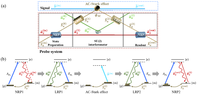
Figure 1: (a) Schematic of QND measurement of photon number. The probe system consists of an SU(1,1)-SU(2)-concatenated atom-light hybrid interferometer. In the SU(2) interferometer in the middle box, the LRP is utilized to realize the splitting and combination of the atomic spin wave and the optical wave. $\hat{a}_{W}^{(0)}$ is a coherent state, $\hat{S}_{a}^{(0)}$, $\hat{S}_{a}^{(1)}$ and $\hat{S}_{a}^{(3)}$ are the atomic collective excitation which are prepared by the NRP1, LRP1 and LRP2, respectively. The atomic spin wave $\hat{S}_{a}^{(1)}$ experiences a phase modulation $\phi_{AC}$ via the AC-Stark effect by signal light $\hat{b}^{(in)}$ and evolves to $\hat{S}_{a}^{(2)}$. The generated atomic spin wave $\hat{S}_{a}^{(3)}$ of the SU(2) interferometer and the optical wave $\hat{a}_{S}^{(1)}$ which is correlated with $\hat{S}_{a}^{(0)}$ are combined to realize active correlation output readout via the NRP2. $\mathrm{LRP}$, linear Raman process; $\mathrm{NRP}$, nonlinear Raman process. (b) Energy levels of the atom. The lower two energy states $|g\rangle$ and $|m\rangle$ are the hyperfine split ground states. The higher-energy state $|e\rangle$ is the excited state. The strong pump field $A_{p_{1}}$ ($A_{p_{2}}$) and strong read field $E_{p_{1}}$ ($E_{p_{2}}$) couple the transitions $|g\rangle$ $\rightarrow$ $|e\rangle$ and $|m\rangle$ $\rightarrow$ $|e\rangle$, respectively. $\hat{b}^{(in)}$ is far off resonance with the transition $|m\rangle$ $\rightarrow$ $|e\rangle$ by a large detuning.

In the quantum optics community, Imoto et al. [15] proposed an optical interferometer for QND measurement scheme of the photon number using the optical Kerr effect, in which the cross-Kerr interaction encodes the photon number of the signal state onto a phase shift of the probe state. Subsequently, some works about the photon number QND measurement are studied [16, 17, 18, 19, 20, 21]. However, the main obstacles to optical QND measurement using cross-phase modulation based on third-order nonlinear susceptibilities $\chi^{(3)}$ are the small value of nonlinearity in the available media and the absorption of photons. Munro et al. [22] presented an implementation of the QND measurement scheme with the required nonlinearity provided by the giant Kerr effect achievable with AC-Stark electromagnetically transparency. In addition, the schemes using cavity or circuit quantum electrodynamical systems have enabled photon number QND measurements that do not rely on the material nonlinearity through strong light-matter interactions [23, 24, 25, 26, 27].

Interferometric measurements allow for highly sensitive detection of any small changes that induces an optical phase shift. Different kinds of quantum interferometers have been proposed for phase measurement [28, 29, 30, 31, 32, 33, 34, 35, 36, 37]. The phase sensitivity of the SU(2) interferometer with coherent state input, such as the Michelson or Mach-Zehnder interferometer, is limited by the shot noise limit. When the unused port of the interferometer is fed with squeezed state, the SU(2) interferometer can beat this limit [28]. In contrast to the SU(2) interferometer, the SU(1,1) nonlinear interferometer that replaces the beam splitters in the SU(2) interferometer with nonlinear gain media is a fundamentally different type of interferometric detector [29], in which the quantum correlations are generated within the interferometer, the phase sensitivity can, in principle, approach the Heisenberg limit.

Recently, using the coherent mixing of an optical wave and an atomic spin wave, the atom-light hybrid interferometer has been proposed and studied [38, 39, 40, 41, 42, 43, 44]. Similarly, there are two types of atom-light hybrid interferometers, which have been also demonstrated experimentally. One is SU(2)-type atom-light hybrid interferometer [40], where the linear Raman processes (LRPs) replace the beam splitters in the SU(2) linear interferometer to realize linear superposition of atomic wave and optical wave. The other is SU(1,1)-type atom-light hybrid interferometer [41], where the nonlinear Raman processes (NRPs) realize the atomic wave and optical wave splitting and recombination. The atom-light hybrid interferometer has drawn considerable interest because it is sensitive to both optical and atomic phase shift. Resorting to an AC Stark effect for the atomic phase change, the atom-light hybrid interferometer can be applied to QND measurement of photon number [45, 46]. Further developing methods to improve the measurement procision is always desired for the innovation of interferometers.

In this paper, we present an SU(1,1)-SU(2)-concatenated atom-light hybrid interferometer, which is combination of SU(2) and SU(1,1) type atom-light hybrid interferometers. Then the AC-Stark effect encodes the photon number of the signal light onto a phase shift of the atomic spin wave, so that the problem of detecting photon number is translated into the problem of detecting the atomic phase shift. Thus we theoretically analyze the SNR of the interferometer for precision measurement of the phase shift to examine the performance of this scheme as a QND measurement. Besides, an ideal QND measurement can be testified by a perfect correlation between the signal light and the probe system [47]. Here we estimate the quality of QND measurement using the criteria in Ref. [47], and the condition for a perfect correlation is given. In the presence of losses, the measurement quality is reduced. However, we can adjust the gain parameter of the NRP in readout stage to reduce the impact due to losses.

Our scheme can be thought of as inserting an SU(2)-type atom-light hybrid interferometer into one of the arms of the SU(1,1)-type atom-light hybrid interferometer. Compared to a conventional SU(1,1) interferometer, the number of phase-sensing particles is further increased due to input field $\hat{a}_{W}^{(0)}$. In the previous scheme [45], a strong stimulated Raman process can indeed be used to excite most of the atoms to the $|m\rangle$ state to improve the number of phase-sensing particles. However, this will produce additional nonlinear effects and noise light fields [48, 49, 50]. Therefore, in the current scheme, firstly a spontaneous Raman process is used, and then a LRP is used to generate the Rabi-like superposition oscillation between light and the atom. By controlling the interaction time, more atoms can be prepared to the $|m\rangle$ state to improve the number of phase-sensing particles to enhance the QND measurement. Compared to the previous works [45, 46], the SU(1,1)-SU(2)-concatenated atom-light hybrid interferometer can be realized QND measurement of photon number with higher precision. Since the SU(2)-type and SU(1,1)-type atom-light hybrid interferometers [40, 41] have been demonstrated experimentally, the SU(1,1)-SU(2)-concatenated atom-light hybrid interferometer could be realized with current experimental conditions and the corresponding experimental requirements are given in the discussion part.

2 An SU(1,1)-SU(2)-concatenated Atom-light hybrid interferometer

An SU(1,1)-SU(2)-concatenated atom-light hybrid interferometer is shown in Fig. 1 (a). The corresponding energy levels of atom and optical frequencies for the formation of the SU(1,1)-SU(2)-concatenated atom-light hybrid interferometer are given in Fig. 1 (b), where the lower two energy states $|g\rangle$ and $|m\rangle$ are the hyperfine split ground states. The higher-energy state $|e\rangle$ is the excited state. The strong pump field $A_{p_{1}}$ ($A_{p_{2}}$) and strong read field $E_{p_{1}}$ ($E_{p_{2}}$) couple the transitions $|g\rangle$ $\rightarrow$ $|e\rangle$ and $|m\rangle$ $\rightarrow$ $|e\rangle$, respectively. The process can be used to describe the linear and nonlinear splitting and recombination of the light field and spin wave, i.e., NRP and LRP.

In the case of undepleted read field approximation, the two-mode coupled Hamiltonian is written as [40]

$$\hat{H}_{LRP}=i\hbar\Omega\hat{a}_{W}\hat{S}_{a}^{\dagger}+H.c.,$$ (1)

where $\hat{S}_{a}\equiv(1/\sqrt{N})\sum_{k}|g\rangle_{kk}\langle m|$ is the spin wave (atomic collective excitation) with $N$ the number of atoms in the ensemble, and $\Omega$ is the Rabi-like frequency. The Rabi-like oscillation between the write field and the atomic spin wave occurs, and the input-output relation is given by

$$\hat{S}_{a}^{(out)}=\hat{S}_{a}^{(in)}cos(|\Omega|\tau_{r})-\hat{a}_{W}^{(in)}sin(|\Omega|\tau_{r}),$$

$$\hat{a}_{W}^{(out)}=\hat{a}_{W}^{(in)}cos(|\Omega|\tau_{r})+\hat{S}_{a}^{(in)}sin(|\Omega|\tau_{r}),$$ (2)

where $\tau_{r}$ is the interaction time of read field $E_{p}$. This transform of Eq. (2) can be used for LRP. In the case of undepleted pump field approximation, the Hamiltonian is written as [41]

$$\hat{H}_{NRP}=i\hbar{\eta}A_{p}\hat{a}_{S}^{{\dagger}}\hat{S}_{a}^{{\dagger}}+H.c.,$$ (3)

where $\eta$ is the coupling coefficient, and $A_{p}$ is the amplitude of the pump beam. The input-output relation is given by

$$\hat{S}_{a}^{(out)}=G\hat{S}_{a}^{(in)}+ge^{i\theta}\hat{a}_{S}^{\dagger(in)},\text{ }\hat{a}_{S}^{(out)}=G\hat{a}_{S}^{(in)}+ge^{i\theta}\hat{S}_{a}^{\dagger(in)},$$ (4)

where $e^{i\theta}=\eta A_{p}/|\eta A_{p}|$, $G=\cosh(|\eta A_{p}|\tau_{p})$ and $g=\sinh(|\eta A_{p}|\tau_{p})$ are the gains of the process with $G^{2}-g^{2}=1$, $\tau_{p}$ the pulse duration of pump beam $A_{p}$. This transform of Eq. (4) can be used for NRP.

Next, according to above linear and nonlinear transforms, the output operators of the SU(1,1)-SU(2)-concatenated atom-light hybrid interferometer is worked out as a function of the input operators with three steps: (1) the state preparation; (2) the SU(2) interferometer, (3) the readout. In the first step, we prepare the initial atomic spin wave $\hat{S}_{a}^{(0)}$ and a correlated optical wave $\hat{a}_{S}^{(1)}$ via the NRP1. It can be described as

$$\hat{S}_{a}^{(0)}=G_{1}\hat{S}_{a}^{(in)}+g_{1}e^{i\theta_{1}}\hat{a}_{S}^{\dagger(in)},\text{ }\hat{a}_{S}^{(1)}=G_{1}\hat{a}_{S}^{(in)}+g_{1}e^{i\theta_{1}}\hat{S}_{a}^{\dagger(in)}.$$ (5)

Next, the beam splitter in a SU(2) interferometer is provided by the LRP, which can split and mix the atomic spin wave and the optical wave coherently for interference. $\hat{a}_{W}^{(0)}$ is a coherent state, $\hat{S}_{a}^{(0)}$ is an atomic collective excitation which is prepared by the NRP1. The relationship between input and output in the SU(2) interferometer is given by

$$\hat{S}_{a}^{(3)}=t\hat{S}_{a}^{(0)}+r\hat{a}_{W}^{(0)},\text{ }\hat{a}_{W}^{(2)}=t\hat{a}_{W}^{(0)}+r\hat{S}_{a}^{(0)},$$ (6)

where $t=e^{i\phi/2}\cos(\phi/2)$, $r=ie^{i\phi/2}\sin(\phi/2)$. $\phi$ denotes the phase shift.

In the final step, the generated atomic spin wave $\hat{S}_{a}^{(3)}$ of the SU(2) interferometer and the optical wave $\hat{a}_{S}^{(1)}$ are combined to realize active correlation output readout via the NRP2. It can be expressed as

$$\hat{S}_{a}^{(out)}=G_{2}\hat{S}_{a}^{(3)}+g_{2}e^{i\theta_{2}}\hat{a}_{S}^{\dagger(1)},\text{ }\hat{a}_{S}^{(out)}=G_{2}\hat{a}_{S}^{(1)}+g_{2}e^{i\theta_{2}}\hat{S}_{a}^{\dagger(3)}.$$ (7)

And thus, the full input-output relation of the actively correlated atom-light hybrid interferometer is

$$\hat{a}_{S}^{(out)} =A\hat{a}_{S}^{(in)}+B\hat{S}_{a}^{\dagger(in)}+C\hat{a}_{W}^{\dagger(0)},$$

$$\hat{S}_{a}^{(out)} =D\hat{a}_{S}^{\dagger(in)}+E\hat{S}_{a}^{(in)}+F\hat{a}_{W}^{(0)},$$ (8)

where

$$A =G_{2}G_{1}+g_{2}g_{1}e^{i(\theta_{2}-\theta_{1})}t^{\ast},\text{ }B=G_{2}g_{1}e^{i\theta_{1}}+G_{1}g_{2}e^{i\theta_{2}}t^{\ast},$$

$$D =G_{1}g_{2}e^{i\theta_{2}}+G_{2}g_{1}e^{i\theta_{1}}t,\text{ }E=g_{2}g_{1}e^{i(\theta_{2}-\theta_{1})}+G_{2}G_{1}t,$$

$$C =g_{2}e^{i\theta_{2}}r^{\ast},\text{ }F=G_{2}r.$$ (9)

3 QND measurement of photon number

This new type interferometer in Section 2 can be used as a probe system for QND measurement. The schematic of QND measurement of photon number is shown in Fig. 1 (a), when the atoms system of this new type interferometer are illuminated by the off-resonant signal light $\hat{b}^{(in)}$, the interaction between atom and signal light $\hat{b}^{(in)}$ will induce an atomic phase shift [51, 52]

$$\phi_{AC}=\kappa\hat{n}_{b},$$ (10)

where $\hat{n}_{b}=\hat{b}^{(in){\dagger}}\hat{b}^{(in)}$ is photon number operator of the signal light and $\kappa$ is the AC-Stark coefficient.

In this QND measurement scheme, the photon number of the signal light is the QND observable, while the phase of the signal light is the conjugated observable. The quantum noise induced by the act of measurement is fed into the unmeasured conjugate observable $\phi^{(s)}$ of the signal light, where superscript $(s)$ denotes the signal light. The uncertainty of these two observables is limited by the Heisenberg relation $\Delta n_{b}^{(s)}\Delta\phi^{(s)}\geq 1$ [53]. That is, the QND measurement of the observable $n_{b}^{(s)}$ is accomplished at the expense of uncertainty increasement of its conjugate observable $\phi^{(s)}$. By monitoring the atomic phase shift $\phi_{AC}$ using this atom-light hybrid interferometer, we can determine the photon number of the signal light without destroying the photons. The phase shift of the atomic spin wave is the readout observable, which can be measured by the homodyne detection. Next, we analyze the performance of this scheme as a QND measurement.

3.1 SNR analysis

The QND measurement scheme that uses the AC-Stark effect is based on the precision measurement of the photon-induced atomic phase shift, thus the SNR analysis is helpful to examine the performance of the QND measurement process. Given the homodyne detection, the SNR is defined as

$$R=\frac{\langle\hat{X}_{S}^{(out)}\rangle^{2}}{\langle\Delta^{2}\hat{X}_{S}^{(out)}\rangle},$$ (11)

where $\langle\hat{X}_{S}^{(out)}\rangle$ and $\langle\Delta^{2}\hat{X}_{S}^{(out)}\rangle$ denote the quantum expectation and variance of the amplitude quadrature, respectively. In our scheme, they are given by

$$\langle\hat{X}_{S}^{(out)}\rangle =\langle\hat{a}_{S}^{(out)}+\hat{a}_{S}^{\dagger(out)}\rangle$$

$$=g_{2}N_{\alpha}^{1/2}[\cos(\theta_{2}-\theta_{\alpha}-\phi)-\cos(\theta_{2}-\theta_{\alpha})].$$ (12)

$$\langle\Delta^{2}\hat{X}_{S}^{(out)}\rangle =G_{2}^{2}G_{1}^{2}+G_{2}^{2}g_{1}^{2}+g_{2}^{2}(1-\cos\phi)/2$$

$$+g_{2}^{2}g_{1}^{2}(1+\cos\phi)/2+G_{1}^{2}g_{2}^{2}(1+\cos\phi)/2$$

$$+2G_{2}G_{1}g_{2}g_{1}\cos(\theta_{2}-\theta_{1}-\phi)$$

$$+2G_{2}G_{1}g_{2}g_{1}\cos(\theta_{2}-\theta_{1}).$$ (13)

Here $\hat{a}_{S}^{(in)}$ and $\hat{S}_{a}^{(in)}$ are in vacuum states, $\hat{a}_{W}^{(0)}$ is in a coherent state $|\alpha\rangle$ with $\alpha=N_{\alpha}^{1/2}e^{i\theta_{\alpha}}$ where $N_{\alpha}$ and $\theta_{\alpha}$ are the photon number and initial phase of the coherent state, respectively. The phase shift $\phi$ includes the phase difference $\phi_{0}$ of the interferometer and the phase difference $\phi_{AC}$ caused by the AC-Stark effect with $\phi_{AC}=\kappa\hat{n}_{b}$. Our scheme can be thought of as inserting a SU(2) interferometer into one of the arms of the SU(1,1) interferometer. For a balanced SU(1,1) interferometer configuration, two NRPs of equal gain ($g_{2}=g_{1}=g$) and opposite pump phases ($\theta_{1}=0$, $\theta_{2}=\pi$) are arranged in series. NRP1 produces an optical field together with a correlated atomic spin excitation, while NRP2 is shifted in pump phase to exactly reverse the operation of NRP1 and return the optical field and atomic spin excitation back to their original input states. When a phase shift is introduced, the transfer is no longer complete, and thus lead to a change in the output corresponding to the induced phase shift. Here we first consider a balanced case in which the SU(2) interferometer is introduced into a balanced SU(1,1) interferometer. With a small $\phi_{AC}$ around $\phi_{0}=0$ and $\alpha=iN_{\alpha}^{1/2}$, assuming the signal light is in a number state $|n\rangle$ with $\hat{n}_{b}|n\rangle=n_{b}|n\rangle$ and substituting $\phi_{AC}$ with $\kappa\hat{n}_{b}$, the SNR is

$$R\approx g^{2}\kappa^{2}N_{\alpha}n_{b}^{2}.$$ (14)

To have single-photon resolution, we need AC-Stark coefficient $\kappa\sim 1/gN_{\alpha}^{1/2}$. Compared to the traditional SU(2) interferometer [45], the required coefficient is smaller by a factor of $1/g$ . This is due to the method of active correlation output readout for the SU(2) interferometer [54], in which the SNR is greater than the SU(2) interferometer by a factor of $g$ of NRP.

3.2 Quality estimation

In the QND measurement, the signal light is coupled to the probe system, and a subsequent readout measurement of the probe output is made to extract the information about the signal light without perturbing it. An ideal QND measurement requires a perfect correlation between the signal and the probe system. In practice, the probe output itself has fluctuation, which leads to a nonideal QND measurement. Thus the quality of the QND measurement scheme is worth studying. In this section, we estimate the quality using the criteria introduced by Holland et al. [47], which are

$$C_{S^{in}S^{out}}^{2} =\frac{|\langle S^{in}S^{out}\rangle-\langle S^{in}\rangle\langle S^{out}\rangle|^{2}}{\langle\Delta^{2}S^{in}\rangle\langle\Delta^{2}S^{out}\rangle},$$ (15)

$$C_{S^{in}P^{out}}^{2} =\frac{|\langle S^{in}P^{out}\rangle-\langle S^{in}\rangle\langle P^{out}\rangle|^{2}}{\langle\Delta^{2}S^{in}\rangle\langle\Delta^{2}P^{out}\rangle},$$ (16)

$$C_{S^{out}P^{out}}^{2} =\frac{|\langle S^{out}P^{out}\rangle-\langle S^{out}\rangle\langle P^{out}\rangle|^{2}}{\langle\Delta^{2}S^{out}\rangle\langle\Delta^{2}P^{out}\rangle},$$ (17)

with

$$\langle\Delta^{2}S^{in}\rangle =\langle(S^{in})^{2}\rangle-\langle S^{in}\rangle^{2},$$

$$\langle\Delta^{2}S^{out}\rangle =\langle(S^{out})^{2}\rangle-\langle S^{out}\rangle^{2},$$

$$\langle\Delta^{2}P^{in}\rangle =\langle(P^{in})^{2}\rangle-\langle P^{in}\rangle^{2},$$

$$\langle\Delta^{2}P^{out}\rangle =\langle(P^{out})^{2}\rangle-\langle P^{out}\rangle^{2},$$ (18)

where $S^{in}$ is the input signal incident on the scheme and $P^{out}$ is the output probe measured by a detector. Here $S^{in}$ is the photon number of the input signal $\hat{N}^{(in)}=\hat{b}^{\dagger(in)}\hat{b}^{(in)}$, and the probe is the amplitude quadrature $\hat{X}_{S}^{(out)}$. Eq. (15) is about how much the probe system degrades the signal of the measured system. Eq. (16) is about how good the probe system is a measurement device. Eq. (17) is that how good the probe system is a state preparation device. For a ideal QND measurement device the correlation coefficients $C_{S^{in}S^{out}}^{2}$, $C_{S^{in}P^{out}}^{2}$ and $C_{S^{out}P^{out}}^{2}$ are unity. In our paper, the signal light leading to the AC-Stark shift is far off resonance with a large detuning, i.e., the photon number of the measured signal light is not changed before and after measurement. So the first criterion is satisfied, the second and the third criteria become same: $C_{\hat{N}^{(in)}\hat{X}_{S}^{(out)}}^{2}=C_{\hat{N}^{(out)}\hat{X}_{S}^{(out)}}^{2}$, that is,

$$C^{2}=\frac{|\langle\hat{N}^{(in)}\hat{X}_{S}^{(out)}\rangle-\langle\hat{N}^{(in)}\rangle\langle\hat{X}_{S}^{(out)}\rangle|^{2}}{\langle\Delta^{2}\hat{N}^{(in)}\rangle\langle\Delta^{2}\hat{X}_{S}^{(out)}\rangle}.$$ (19)

For brevity, we omit the subscript of $C$. In the previous section, even if we assume the signal light is in a number state, which is the eigen-state of the photon number measurement process ($\hat{n}_{b}|n\rangle=n_{b}|n\rangle$). The probe output has fluctuation and does not yield a definite value. Here, for convenience, the signal light is set in a coherent state $|\beta\rangle$ with photon number $N_{\beta}$. We obtain

$$\langle\hat{N}^{(in)}\rangle =N_{\beta},\text{ }\Delta^{2}\hat{N}^{(in)}=N_{\beta},$$

$$\langle\hat{X}_{S}^{(out)}\rangle =g_{2}\kappa N_{\alpha}^{1/2}N_{\beta},\text{ }\langle\hat{N}^{(in)}\hat{X}_{S}^{(out)}\rangle=g_{2}\kappa N_{\alpha}^{1/2}N_{\beta}(N_{\beta}+1),$$

$$\langle\Delta^{2}\hat{X}_{S}^{(out)}\rangle =(G_{2}G_{1}-g_{2}g_{1})^{2}+(G_{2}g_{1}-G_{1}g_{2})^{2}$$

$$+g_{2}^{2}\kappa^{2}N_{\alpha}N_{\beta}+G_{1}^{2}g_{2}^{2}\kappa^{2}N_{\beta}(N_{\beta}+1)/2.$$ (20)

Substituting Eq. (20) into Eq. (19), the criteria can be written as

$$C^{2}=\frac{1}{1+\frac{(G_{2}G_{1}-g_{2}g_{1})^{2}+(G_{2}g_{1}-G_{1}g_{2})^{2}}{g_{2}^{2}\kappa^{2}N_{\alpha}N_{\beta}}+\frac{G_{1}^{2}(N_{\beta}+1)}{2N_{\alpha}}}.$$ (21)

As seen in Eq. (21), a perfect correlation $C^{2}\approx 1$ can be satisfied under the condition of $g_{2}^{2}\kappa^{2}N_{\alpha}N_{\beta}\gg(G_{2}G_{1}-g_{2}g_{1})^{2}+(G_{2}g_{1}-G_{1}g_{2})^{2}$ and $2N_{\alpha}\gg G_{1}^{2}(N_{\beta}+1)$. In a balanced case, the condition for a perfect correlation is $g^{2}\kappa^{2}N_{\alpha}N_{\beta}\gg 1$ and $2N_{\alpha}\gg G^{2}(N_{\beta}+1)$.

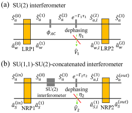
Figure 2: A lossy interferometer model with (a) internal loss and (b) external loss.

3.3 Optimized C in the presence of losses

Next, we investigate the effects of losses on the correlation coefficient $C$ in the presence of photon losses and atomic decoherence losses [43].

The loss of the two arms inside the SU(2) interferometer is called the internal loss, as shown in Fig. 2(a). The loss at the output of SU(2) and the associated optical field is called external loss, as shown in Fig. 2(b). Two fictitious beam splitters are introduced to mimic the loss of photons into the environment, then the optical waves $\hat{a}_{W}^{(1)}$ and $\hat{a}_{S}^{(1)}$ experience losses as

$$\hat{a}_{W,l}^{(1)} =\sqrt{\eta_{1}}\hat{a}_{W}^{(1)}+\sqrt{1-\eta_{1}}\hat{V}_{1},$$ (22)

$$\hat{a}_{S,l}^{(1)} =\sqrt{\eta_{2}}\hat{a}_{S}^{(1)}+\sqrt{1-\eta_{2}}\hat{V}_{2},$$ (23)

where subscript $l$ indicates the loss, $\eta_{1}$ ($\eta_{2}$) and $\hat{V}_{1}$ ($\hat{V}_{2}$) represent the transmission rate and vacuum, respectively. The spin waves $\hat{S}_{a}^{(2)}$ ($\hat{S}_{a}^{(3)}$) also undergoes the collisional dephasing $e^{-\Gamma_{1}\tau_{1}}$ ($e^{-\Gamma_{2}\tau_{2}}$), then the spin waves are described by

$$\hat{S}_{a,l}^{(2)} =\hat{S}_{a}^{(2)}e^{-\Gamma_{1}\tau_{1}}+\hat{F}_{1},$$ (24)

$$\hat{S}_{a,l}^{(3)} =\hat{S}_{a}^{(3)}e^{-\Gamma_{2}\tau_{2}}+\hat{F}_{2},$$ (25)

where $\langle\hat{F}_{1}\hat{F}_{1}^{\dagger}\rangle=1-e^{-2\Gamma_{1}\tau_{1}}$ and $\langle\hat{F}_{2}\hat{F}_{2}^{\dagger}\rangle=1-e^{-2\Gamma_{2}\tau_{2}}$ guarantees the consistency of the operator properties of $\hat{S}_{a,l}^{(2)}$ and $\hat{S}_{a,l}^{(3)}$, respectively. The input-output relation for loss case of $\hat{a}_{S}^{(out)}$ becomes

$$\hat{a}_{S,l}^{(out)} =\hat{a}_{S}^{(in)}\mathcal{A}+\hat{S}_{a}^{\dagger(in)}\mathcal{B}+\hat{a}_{W}^{\dagger(0)}\mathcal{C}+\hat{V}_{1}^{\dagger}\mathcal{D}+\hat{V}_{2}\mathcal{E}$$

$$+\hat{F}_{1}^{\dagger}\mathcal{F}+\hat{F}_{2}^{\dagger}\mathcal{G},$$ (26)

where

$$\mathcal{A} =[\sqrt{\eta_{2}}G_{2}G_{1}+g_{2}g_{1}e^{i(\theta_{2}-\theta_{1})}(e^{-\Gamma_{1}\tau_{1}}e^{-i\phi}+\sqrt{\eta_{1}})e^{-\Gamma_{2}\tau_{2}}/2],$$

$$\mathcal{B} =[\sqrt{\eta_{2}}G_{2}g_{1}e^{i\theta_{1}}+G_{1}g_{2}e^{i\theta_{2}}(e^{-\Gamma_{1}\tau_{1}}e^{-i\phi}+\sqrt{\eta_{1}})e^{-\Gamma_{2}\tau_{2}}/2],$$

$$\mathcal{C} =g_{2}e^{i\theta_{2}}(e^{-\Gamma_{1}\tau_{1}}e^{-i\phi}-\sqrt{\eta_{1}})e^{-\Gamma_{2}\tau_{2}}/2,$$

$$\mathcal{D} =-g_{2}e^{i\theta_{2}}\sqrt{1-\eta_{1}}e^{-\Gamma_{2}\tau_{2}}/\sqrt{2},$$

$$\mathcal{E} =G_{2}\sqrt{1-\eta_{2}},\mathcal{F}=g_{2}e^{i\theta_{2}}e^{-\Gamma_{2}\tau_{2}}/\sqrt{2},\mathcal{G}=g_{2}e^{i\theta_{2}}.$$ (27)

We study the effect of losses under the condition of $\theta_{1}=0$, $\theta_{2}=\pi$, $\theta_{\alpha}=\pi/2$, and $\phi_{0}=0$ with a small $\phi_{AC}$ around $\phi_{0}$. Considering losses the terms of $\langle\hat{X}_{S}^{(out)}\rangle_{l}$, $\langle\hat{N}^{(in)}\hat{X}_{S}^{(out)}\rangle_{l}$, and $\langle\Delta^{2}\hat{X}_{S}^{(out)}\rangle_{l}$ in Eq. (20) are given by

$$\langle\hat{X}_{S}^{(out)}\rangle_{l}=g_{2}e^{-\Gamma_{1}\tau_{1}}e^{-\Gamma_{2}\tau_{2}}\kappa N_{\alpha}^{1/2}N_{\beta},$$ (28)

$$\langle\hat{N}^{(in)}\hat{X}_{S}^{(out)}\rangle_{l}=g_{2}e^{-\Gamma_{1}\tau_{1}}e^{-\Gamma_{2}\tau_{2}}\kappa N_{\alpha}^{1/2}N_{\beta}(N_{\beta}+1),$$ (29)

and

$$\langle\Delta^{2}\hat{X}_{S}^{(out)}\rangle_{l}$$

$$=(\sqrt{\eta_{2}}G_{2}G_{1}-g_{2}g_{1}e^{-\Gamma_{1}\tau_{1}}e^{-\Gamma_{2}\tau_{2}}/2-g_{2}g_{1}e^{-\Gamma_{2}\tau_{2}}\sqrt{\eta_{1}}/2)^{2}$$

$$+(\sqrt{\eta_{2}}G_{2}g_{1}-G_{1}g_{2}e^{-\Gamma_{1}\tau_{1}}e^{-\Gamma_{2}\tau_{2}}/2-G_{1}g_{2}e^{-\Gamma_{2}\tau_{2}}\sqrt{\eta_{1}}/2)^{2}$$

$$+g_{2}^{2}[(1-e^{-2\Gamma_{1}\tau_{1}})e^{-2\Gamma_{2}\tau_{2}}/2+(1-e^{-2\Gamma_{2}\tau_{2}})]$$

$$+g_{2}^{2}(2g_{1}^{2}+1)\kappa^{2}N_{\beta}(N_{\beta}+1)e^{-2\Gamma_{1}\tau_{1}}e^{-2\Gamma_{2}\tau_{2}}/4$$

$$+g_{2}^{2}\kappa^{2}N_{\beta}[N_{\alpha}+(N_{\beta}+1)/4]e^{-2\Gamma_{1}\tau_{1}}e^{-2\Gamma_{2}\tau_{2}}$$

$$+(g_{2}e^{-\Gamma_{2}\tau_{2}}\sqrt{\eta_{1}}/2-g_{2}e^{-\Gamma_{1}\tau_{1}}e^{-\Gamma_{2}\tau_{2}}/2)^{2}$$

$$+g_{2}^{2}(1-\eta_{1})e^{-2\Gamma_{2}\tau_{2}}/2+G_{2}^{2}(1-\eta_{2}),$$ (30)

then the QND measurement criterion for loss case can be obtained according to Eq. (19).

In our scheme, the atomic spin wave stays in the atomic ensemble while the optical field travels out of the atomic ensemble. Here, within the coherence time the atomic collisional dephasing loss $\Gamma_{1}\tau_{1}$ ($\Gamma_{2}\tau_{2}$) is small, then we set $e^{-\Gamma_{1}\tau_{1}}=e^{-\Gamma_{2}\tau_{2}}=0.9$. The correlation coefficient $C$ as a function of $\eta_{1}$ and $\eta_{2}$ in balanced case is shown in Fig. 3. It is shown that the reduction in the correlation coefficient $C$ increases as the loss increases. It is shown that our scheme is more tolerant with the internal photon loss $\eta_{1}$ compared to the photon loss outside the SU(2) interferometer $\eta_{2}$. The reason behind the phenomenon is that large external photon loss affects quantum correlation between the light wave and atomic spin wave, which destroys the active correlation output readout.

In the unbalanced case ($g_{1}\neq g_{2}$), we can adjust the gain ratio $g_{2}/g_{1}$ of the beam recombination process to reduce the reduction in correlation coefficient. The black line in Fig. 3 is labeled as $C_{0}$, as a benchmark for comparison before and after optimization, here we set $C_{0}=0.6$. The correlation coefficient in the area of upper right corner and within the $C_{0}$ lines can be kept above $0.6$. After optimizing the $g_{2}$, the correlation coefficient as a function of $\eta_{1}$ and $\eta_{2}$ can also be obtained, where the line with $C$ equal to $0.6$ is denoted as $C_{1}$. The contour line of optimized $g_{2}/g_{1}$ as a function of $\eta_{1}$ and $\eta_{2}$ are shown in Fig. 4, where the position of $C_{0}$ (before optimization) and $C_{1}$ (after optimization) in the contour figure of the correlation coefficient versus transmission rates has changed. It is demonstrated that for a given $g_{1}$ by optimizing $g_{2}/g_{1}$, the small area between the $C_{0}$ and $C_{1}$ can still kept above $0.6$. That is within a certain losses range, $C$ can continue to beat the criteria (such as $C$ equal to $0.6)$ after optimizing $g_{2}/g_{1}$. The newly added area after optimization is divided into two parts, one of which is the ratio $g_{2}/g_{1}$ within the very small area above is less than 1, and the other part the ratio $g_{2}/g_{1}$ needs to be greater than 1.

4 Discussion and Conclusion

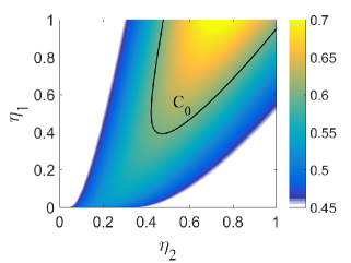
Figure 3: Correlation coefficient $C$ as a function of $\eta_{1}$ and $\eta_{2}$, where $e^{-\Gamma_{1}\tau_{1}}=e^{-\Gamma_{2}\tau_{2}}=0.9$, $\kappa=10^{-10}$, $g_{1}=g_{2}=3$, $N_{\alpha}=10^{12}$, and $N_{\beta}=10^{8}$. The correlation coefficient in the area of upper right corner and within the $C_{0}$ lines can be kept above 0.6.

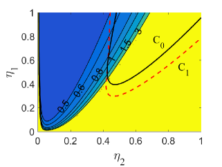
Figure 4: Contour line of optimized $g_{2}/g_{1}$ as a function of $\eta_{1}$ and $\eta_{2}$ with $e^{-\Gamma_{1}\tau_{1}}=e^{-\Gamma_{2}\tau_{2}}=0.9$, where $\kappa=10^{-10}$, $g_{1}=3$, $N_{\alpha}=10^{12}$, and $N_{\beta}=10^{8}$. The correlation coefficient in the area of upper right corner and within the line $C_{0}$ (before optimization) or $C_{1}$ (after optimization) can be kept above $0.6$.

In our scheme, the spin wave prepared by the first NRP participates in the subsequent LRP and NRP and additional operations are required within the coherence time of the spin wave compared to previous experimental works on atom-light interferometers [40, 41], therefore the pulse width and intensity of the pump field $A_{p_{1}}$ ($A_{p_{2}}$) and the read field $E_{p_{1}}$ ($E_{p_{2}}$) should be properly arranged. Experimental consideration of the implementation of the scheme may be performed with a rubidium atomic vapor in a cell. The energy levels of the Rb atom are shown in Fig. 1 (b), where states $|g\rangle$ and $|m\rangle$ are the two ground states $|5^{2}S_{1/2},F=1,2\rangle$ from hyperfine splitting and $|e\rangle$ is the excited state $|5^{2}P_{1/2},F=2\rangle$. The signal field is far resonance with the transition $|5^{2}S_{1/2},F=2\rangle$ $\rightarrow$ $|5^{2}P_{1/2},F=2\rangle$ by $2-4$ GHz detuning [40]. The interaction between atom and signal light will induce an atomic phase shift which is proportional to the photon number of the signal field. With a detuning 2 GHz and photon number of signal light $N_{\beta}=10^{8}$, the AC Stark coupling coefficient $\kappa$ is $\sim 10^{-10}$ rad per photon [45]. With a gain $g^{2}=10$ obtained by turning the pumping field intensity, to realize a perfect correlation the theoretical requirement $N_{\alpha}N_{\beta}\gg(1/g\kappa)^{2}=10^{19}$ and $N_{\alpha}\gg 5.5N_{\beta}$ should be satisfied. Since given $N_{\beta}=10^{8}$, we choose $N_{\alpha}=10^{12}$. In the calculations, the photon numbers are much smaller than the number of atoms in the interaction region. Thus, the density of the atomic sample is $10^{13}$-$10^{14}$/$cm^{3}$ by controlling the cell temperature. The signal light is turned on after the first linear Raman splitting process and turned off right before the second linear Raman mixing process. The pulse width of signal light should be short, and in this way, it will not affect the LRP for splitting and mixing the atomic and optical waves. Here, we set the pulse width of signal field $\sim$100 ns. To realize $N_{\beta}=10^{8}$, the power of signal light is $\sim$0.25 mW for wavelength 0.795 $\mu m$ with coherent time 100 $ns$. The mean photon number $N_{\alpha}=10^{12}$ of $\hat{a}_{W}^{(0)}$ field is given with $\sim$2.5 mW of coherent time 100 $\mu s$ for wavelength 0.795 $\mu m$. The requirement for the number of photons $N_{\alpha}$ and $N_{\beta}$ can be met and be feasible in the experiment.

In conclusion, we have proposed an SU(1,1)-SU(2)-concatenated atom-light hybrid interferometer and used it for QND measurement of photon number via the AC-Stark effect. In the scheme, the atomic spin wave of the SU(2) interferometer is prepared via a NRP and the output is detected with the method of active correlation output readout via another NRP. Benefiting from that, the SNR in the balanced case is improved by a factor of $g$ compared to the traditional SU(2) interferometer. The condition for a perfect correlation is given. The measurement quality is reduced in the presence of losses. We can adjust the gain parameter of the NRP in readout stage to reduce the impact of losses. Moreover, the scheme is a multi-arm interferometer and it provides an option for the simultaneous estimation of more than two parameters with a wide range of applications, such as phase imaging [55], quantum sensing networks [56], the detection of vector fields [57] and so on.

Funding

This work is supported by Development Program of China Grant No. 2016YFA0302001; National Natural Science Foundation of China Grants No. 11974111, No. 11874152, No. 91536114, No. 11574086, No. 11974116, No. 11654005; Shanghai Rising-Star Program Grant No. 16QA1401600; Innovation Program of Shanghai Municipal Education Commission No. 202101070008E00099; the Shanghai talent program, the Chinese National Youth Talent Support Program, and the Fundamental Research Funds for the Central Universities.

Disclosures

The authors declare no conflicts of interest.

References

- [1] C. M. Caves, K. S. Thorne, R. W. P. Drever, V. D. Sandberg and M. Zimmermann, “On the measurement of a weak classical force coupled to a quantum-mechanical oscillator. I. Issues of principle," Rev. Mod. Phys. 52, 341-392 (1980).
- [2] M. F. Bocko, and R. Onofrio, “On the measurement of a weak classical force coupled to a harmonic oscillator: experimental progress." Rev. Mod. Phys. 68, 755-799 (1996).
- [3] V. B. Braginsky and F. Ya. Khalili, “Quantum nondemolition measurements: The route from toys to tools," Rev. Mod. Phys. 68, 1-11 (1996).
- [4] F. Lecocq, J. B. Clark, R. W. Simmonds, J. Aumentado, and J. D. Teufel, “Quantum Non-Demolition Measurement of a Nonclassical State of a Massive Object," Phys. Rev. X 5, 041037 (2015).
- [5] M. Rossi, D. Mason, J. Chen, Y. Tsaturyan, and A. Schliesser, “Measurement-Based Quantum Control of Mechanical Motion," Nature (London) 563, 53-58 (2018).
- [6] D. B. Hume, T. Rosenband, and D. J. Wineland, “High-Fidelity Adaptive Qubit Detection through Repetitive Quantum Non-Demolition Measurements," Phys. Rev. Lett. 99, 120502 (2007).
- [7] F. Wolf, Y. Wan, J. C. Heip, F. Gebert, C. Shi, and P. O. Schmidt, “Non-Destructive State Detection for Quantum Logic Spectroscopy of Molecular Ions," Nature (London) 530, 457-460 (2016).
- [8] M. Raha, S. Chen, C. M. Phenicie, S. Ourari, A. M. Dibos, and J. D. Thompson, “Optical Quantum Non-Demolition Measurement of a Single Rare Earth Ion Qubit," Nat. Commun. 11, 1-6 (2020).
- [9] X. Xue, B. D’Anjou, T. F. Watson, D. R. Ward, D. E. Savage, M. G. Lagally, M. Friesen, S. N. Coppersmith, M. A. Eriksson, W. A. Coish, and L. M. K. Vandersypen, “Repetitive Quantum Non-Demolition Measurement and Soft Decoding of a Silicon Spin Qubit," Phys. Rev. X 10, 021006 (2020).
- [10] S. Hacohen-Gourgy, L. S. Martin, E. Flurin, V. V. Ramasesh, K. B. Whaley, and I. Siddiqi, “Quantum Dynamics of Simultaneously Measured Non-Commuting Observables," Nature (London) 538, 491-494 (2016).
- [11] U. Vool, S. Shankar, S. O. Mundhada, N. Ofek, A. Narla, K. Sliwa, E. Zalys-Geller, Y. Liu, L. Frunzio, R. J. Schoelkopf, S. M. Girvin, and M. H. Devoret, “Continuous Quantum Non-Demolition Measurement of the Transverse Component of a Qubit," Phys. Rev. Lett. 117, 133601 (2016).
- [12] P. Grangier, J. A. Levenson, and J.-P. Poizat, “Quantum non-demolition measurements in optics,"Nature (London) 396, 537-542 (1998).
- [13] A. Reiserer, S. Ritter, and G. Rempe, “Non-Destructive Detection of an Optical Photon," Science 342, 1349-1351 (2013).
- [14] S. Kono, K. Koshino, Y. Tabuchi, A. Noguchi, and Y. Nakamura, “Quantum Non-Demolition Detection of an Itinerant Microwave Photon," Nat. Phys. 14, 546-549 (2018).
- [15] N. Imoto, H. A. Haus, and Y. Yamamoto, “Quantum nondemolition measurement of the photon number via the optical Kerr effect," Phys. Rev. A 32, 2287-2292 (1985).
- [16] M. J. Holland, D. F. Walls, and P. Zoller, “Quantum nondemolition measurements of photon number by atomic beam deflection," Phys. Rev. Lett. 67, 1716-1719 (1991).
- [17] S. R. Friberg, S. Machida, and Y. Yamamoto, “Quantum-nondemolition measurement of the photon number of an optical soliton," Phys. Rev. Lett. 69, 3165-3168 (1992).
- [18] K. Jacobs, P. Tombesi, M. J. Collett, and D. F. Walls, “Quantum-nondemolition measurement of photon number using radiation pressure," Phys. Rev. A 49, 1961-1966 (1994).
- [19] Y. Sakai, R. J. Hawkins, and S. R. Friberg, “Soliton-collision interferometer for the quantum nondemolition measurement of photon number: numerical results," Opt. Lett. 15, 239-241 (1990
- [20] P. Kok, H. Lee and J. P. Dowling, “Single-photon quantum-nondemolition detectors constructed with linear optics and projective measurements," Phys. Rev. A 66, 063814 (2002).
- [21] C. C. Gerry and T. Bui, “Quantum non-demolition measurement of photon number using weak nonlinearities," Phys. Lett. A 372, 7101-7104 (2008).
- [22] W. J. Munro, K. Nemoto, R. G. Beausoleil, and T. P. Spiller, “High-efficiency quantum-nondemolition single-photonnumber-resolving detector," Phys. Rev. A 71, 033819 (2005).
- [23] G. Nogues, A. Rauschenbeutel, S. Osnaghi, M. Brune, J. M. Raimond, and S. Haroche, “Seeing a single photon without destroying it," Nature (London) 400, 239-242 (1999).
- [24] Y. F. Xiao, S. K. Ozdemir, V. Gaddam, C. H. Dong, N. Imoto, and L. Yang, “Quantum nondemolition measurement of photon number via optical Kerr effect in an ultra-high-Q microtoroid cavity," Opt. Express 16, 21462-21475 (2008).
- [25] M. Ludwig, A. H. Safavi-Naeini, O. Painter, and F. Marquardt, “Enhanced Quantum Nonlinearities in a Two-Mode Optomechanical System," Phys. Rev. Lett. 109, 063601 (2012).
- [26] D. Malz and J. I. Cirac, “Nondestructive photon counting in waveguide qed," Phys. Rev. Research 2, 033091 (2020)
- [27] J. Liu, H. T. Chen and D. Segal, “Quantum nondemolition photon counting with a hybrid electromechanical probe," Phys. Rev. A 102, 061501(R) (2020).
- [28] C. M. Caves, “Quantum-mechanical noise in an interferometer," Phys. Rev. D 23, 1693-1708 (1981).
- [29] B. Yurke, S. L. McCall, and J. R. Klauder, “SU(2) and SU(1, 1) interferometers," Phys. Rev. A 33, 4033–4054 (1986).
- [30] L. Pezzé and A. Smerzi, “Mach-Zehnder Interferometry at the Heisenberg Limit with Coherent and Squeezed-Vacuum Light," Phys. Rev. Lett. 100, 073601 (2008).
- [31] J. P. Dowling, “Quantum optical metrology-the lowdown on high-N00N states," Contemp. Phys. 49, 125-143 (2008).
- [32] F. Hudelist, J. Kong, C. Liu, J. Jing, Z. Y. Ou, and W. Zhang, “Quantum metrology with parametric amplifier-based photon correlation interferometers," Nat. Commun. 5, 3049 (2014).
- [33] D. Li, B. T. Gard, Y. Gao, C.-H. Yuan, W. Zhang, H. Lee, and J. P. Dowling, “Phase sensitivity at the Heisenberg limit in an SU(1,1) interferometer via parity detection," Phys. Rev. A 94, 063840 (2016).
- [34] B. E. Anderson, P. Gupta, B. L. Schmittberger, T. Horrom, C. Hermann-Avigliano, K. M. Jones, and P. D. Lett, “Phase sensing beyond the standard quantum limit with a variation on the SU (1, 1) interferometer," Optica 4, 752-756 (2017).
- [35] M. Manceau, G. Leuchs, F. Khalili, and M. Chekhova, “Detection Loss Tolerant Supersensitive Phase Measurement with an SU(1,1) Interferometer," Phys. Rev. Lett. 119, 223604 (2017).
- [36] W. Du, J. Kong, J. Jia, S. Ming, C. H. Yuan, J. F. Chen, Z. Y. Ou, M. W. Mitchell, and W. Zhang, “SU(2)-in-SU(1,1) nested interferometer," arXiv:2004.14266.
- [37] K. Zheng, M. Mi, B. Wang, L. Xu, L. Hu, S. Liu, Y. Lou, J. Jing, and L. Zhang, “Quantum-enhanced stochastic phase estimation with the SU(1,1) interferometer," Photon. Res. 8, 1653-1661 (2020).
- [38] J. Jacobson, G. Björk and Y. Yamamoto, “Quantum limit for the atom-light interferometer," Appl. Phys. B 60, 187-191 (1995).
- [39] G. Campbell, M. Hosseini, B. M. Sparkes, P. K. Lam, and B. C. Buchler, “Time-and frequency-domain polariton interference," New J. Phys. 14, 033022 (2012).
- [40] C. Qiu, S. Chen, L. Q. Chen, B. Chen, J. Guo, Z. Y. Ou, and W. Zhang, “Atom-light superposition oscillation and Ramsey-like atom-light interferometer," Optica 3, 775-780 (2016).
- [41] B. Chen, C. Qiu, S. Chen, J. Guo, L. Q. Chen, Z. Y. Ou, and W. Zhang, “Atom-light hybrid interferometer," Phys. Rev. Lett. 115, 043602 (2015).
- [42] H.-M. Ma, D. Li, C.-H. Yuan, L. Q. Chen, Z. Y. Ou, and W. Zhang, “SU (1, 1)-type light-atom-correlated interferometer," Phys. Rev. A 92, 023847 (2015).
- [43] Z.-D. Chen, C.-H. Yuan, H.-M. Ma, D. Li, L. Q. Chen, Z. Y. Ou, and W. Zhang, “Effects of losses in the atom-light hybrid SU (1, 1) interferometer," Opt. Express 24, 17766-17778(2016).
- [44] S. S. Szigeti, R. J. Lewis-Swan, and S. A. Haine, “Pumped-Up SU(1, 1) Interferometry," Phys. Rev. Lett. 118, 150401 (2017).
- [45] S. Y. Chen, L. Q. Chen, Z. Y. Ou, and W. Zhang, “Quantum non-demolition measurement of photon number with atom-light interferometers," Opt. Express 25, 31827-31839 (2017).
- [46] D. H. Fan, S. Y. Chen, Z. F. Yu, K. Zhang and L. Q. Chen, “Quality estimation of non-demolition measurement with lossy atom-light hybrid interferometers," Opt. Express 28, 9875-9884 (2020).
- [47] M. J. Holland, M. J. Collett, D. F. Walls, and M. D. Levenson, “Nonideal quantum nondemolition measurements," Phys. Rev. A 42, 2995-3005 (1990).
- [48] M. Dabrowski, R. Chrapkiewicz, and W. Wasilewski, “Hamiltonian design in readout from room-temperature Raman atomic memory," Opt. Express 22, 26076-26091 (2014).
- [49] J. Nunn, J. H. D. Munns, S. Thomas, K. T. Kaczmarek, C. Qiu, A. Feizpour, E. Poem, B. Brecht, D. J. Saunders, P. M. Ledingham, D. V. Reddy, M. G. Raymer, and I. A. Walmsley, “Theory of noise suppression in -type quantum memories by means of a cavity," Phys. Rev. A 96, 012338 (2017).
- [50] S. E. Thomas, T. M. Hird, J. H. D. Munns, B. Brecht, and D. J. Saunders, “Raman quantum memory with built-in suppression of four-wave-mixing noise," Phys. Rev. A 100, 033801 (2019).
- [51] S. H. Autler and C. H. Townes, “Stark effect in rapidly varying fields," Phys. Rev. 100, 703-722 (1955).
- [52] K. Hammerer, A. S. Sørensen and E. S. Polzik, “Quantum interface between light and atomic ensembles", Rev. Mod. Phys. 82, 1041-1093 (2010).
- [53] W. Heitler, The Quantum Theory of Radiation (Oxford University, 1954).
- [54] G.-F. Jiao, K. Zhang, L. Q. Chen, W. Zhang and C.-H. Yuan, “Nonlinear phase estimation enhanced by an actively correlated Mach-Zehnder interferometer," Phys. Rev. A 102, 033520 (2020).
- [55] M. Tsang, “Quantum imaging beyond the diffraction limit by optical centroid measurements," Phys. Rev. Lett. 102, 253601 (2009).
- [56] T. J. Proctor, P. A. Knott, and J. A. Dunningham, “Multiparameter estimation in networked quantum sensors," Phys. Rev. Lett. 120, 080501 (2018).
- [57] T. Baumgratz and A. Datta, “Quantum Enhanced Estimation of a Multidimensional Field," Phys. Rev. Lett. 116, 030801 (2016).