EDDA: Explanation-driven Data Augmentation to Improve Explanation Faithfulness

Abstract

Recent years have seen the introduction of a range of methods for post-hoc explainability of image classifier predictions. However, these post-hoc explanations may not always be faithful to classifier predictions, which poses a significant challenge when attempting to debug models based on such explanations. To this end, we seek a methodology that can improve the faithfulness of an explanation method with respect to model predictions which does not require ground truth explanations. We achieve this through a novel explanation-driven data augmentation (EDDA) technique that augments the training data with occlusions inferred from model explanations; this is based on the simple motivating principle that if the explainer is faithful to the model then occluding salient regions for the model prediction should decrease the model confidence in the prediction, while occluding non-salient regions should not change the prediction. To verify that the proposed augmentation method has the potential to improve faithfulness, we evaluate EDDA using a variety of datasets and classification models. We demonstrate empirically that our approach leads to a significant increase of faithfulness, which can facilitate better debugging and successful deployment of image classification models in real-world applications.

Dual submission declaration: This paper has been submitted to the main NeurIPS 2021 conference.

1 Introduction

Deep learning models based on Convolutional Neural Networks(CNNs) have demonstrated superior performance in various computer vision tasks such as image classification [1, 2, 3], object detection [4, 5], and semantic segmentation [6, 7, 8]. However, the interpretability of these models has always been a concern as they often operate as black boxes. Therefore, researchers have recently explored many methodologies for explaining neural networks  [9, 10, 11, 12, 13, 14, 15, 16, 17, 10, 18, 19, 20, 21, 22]. A popular group of post-hoc explanation methods is saliency-based methods [18, 15, 14, 23], which identify the salient regions of the input images through input gradients.

With the development of explanation methodologies, some critical problems arise: What are the desired qualities of a good explainer? And how can we improve the explanation methodologies to have these qualities? Existing works have investigated explanation robustness, where similar inputs should have similar explanations [24, 25, 26]. In this paper, we explore another desired quality of explanation methodologies: faithfulness. Whereas many existing works have explored the idea of faithfulness [26, 27, 28, 29], there is no universal agreement on both its definition and evaluation. In this paper, we believe that a faithful explanation (salient region) related to an input image should contain the crucial information that the classifier utilizes to make the prediction. Therefore, the model should be able to recognize the input with high confidence (we consider here the confidence score as being the softmax probability related to the class predicted by the model [30] after masking the unimportant region according to a faithful explanation (see equation (5))).

(a) Vanilla images

(b) Masking under the classifier trained with no data augmentation

(c) Masking under the classifier trained with EDDA

Figure 1: Example of unfaithful and faithful explanations. (a) The original training images with class whale, mushroom, motorcycle, raccoon and rocket from left to right. (b)The classifier is trained with no data augmentation. After masking out the 50% unimportant regions given by GradCAM, the predicted classes changed into Pine tree, lamp, lamp, lizard and wardrobe accordingly. (c) The classifier is trained with EDDA. After masking out the 50% unimportant regions given by GradCAM, the predicted classes remain to be whale, mushroom, motorcycle, raccoon and rocket accordingly. With EDDA, the explainer successfully identify salient regions that contain the important information for classification.

While providing interpretations of the predictions, the explanations generated by the saliency-based explainers may not always be faithful to the model in question. For example, as shown in Figure 1, after masking the unimportant regions provided by the explainer, the model trained with no augmentation fails to predict the desired label of the image, indicating that the "salient region" provided by the explainer is lacking crucial information for a correct classification. Such cases can easily confuse human users and thus harm the trustworthiness of the model.

In this paper, we aim to improve the faithfulness aspect of the explanations with respect to the model predictions. To accomplish this, we propose explanation-driven data augmentation (EDDA) that augments the training data with occlusions of existing data stemming from model-explanations. Specifically, we generate two occlusions of each input image, namely umask (unimportant-mask) that occludes unimportant/unsalient region and imask (important-mask) that occludes important/salient region. In principle, the prediction of umask images should be the same as the original image and the prediction of imask images should be different. A similar rationale is considered for natural language processing models in [31] where preserving and removing the important parts of the text should respectively keep and alter the model’s decisions accordingly. To verify the effectiveness of our proposed methodology, we conduct experiments on two image datasets (CIFAR-100 [1] and PASCAL VOC 2012 [32]) using two CNN ( ResNet [2] and VGG [3] ) models with GradCAM [23] as the explainer. We empirically demonstrate that EDDA yields more faithful explanations across different datasets and models compared to the non-explanation-driven data augmentation methods.

2 Related Work

Post-hoc Explanations

Post-hoc methods explain the decisions made by a pre-built black-box model. Most of the current post-hoc explanation methods focus on local explanations, which describe the model behavior at the neighborhood of an individual prediction. Early post-hoc explanation methods, such as LIME [17] and SHAP [16], attribute importance scores to input features with respect to the prediction of the target data point. Gradient-based methods are broadly used in explaining Convolutional Neural Networks (CNNs): Saliency Map [18] utilizes the input gradient of the network to highlight the critical pixels for a prediction; Integrated Gradients [15] addresses the gradient saturation issue by generating interpolants from the baseline to the input image and summing over the gradient of each interpolant; SmoothGrad [14] addresses the same issue, and it computes sharper saliency maps by adding noise to copies of the input image and averaging the input gradient of these copies. The Class Activation Map (CAM) [33] based explxanation methods are commonly used in the literature. Grad-CAM [23] employs the weighted activations of the feature maps in the final convolutional layer, where the weights are computed based on the gradient of an output class with respect to each feature map. Despite the variety of these methods, they were either evaluated qualitatively or based on ground truth localization information such as object detection bounding boxes. It may not be meaningful if the dataset is biased, e.g., the classifier can utilize the sea background of the fish objects or the sky background of the plane object to make decisions that overfits specific training data. Recent image-based explanation methods such as Grad-CAM++ [10] and SISE [30] adopt the Drop% and Increase% metrics in the performance evaluation. These metrics capture aspects of faithfulness that we also consider in our work (see equation (5)).

Data Augmentation

Data augmentation is a training strategy that improves the performance of deep learning models by applying various transformations to the original training data. These transformations are relatively simple but effective in increasing the data diversity and the model’s generalization ability. Cutout [19] is a regional dropout method that zero-masks a random fix-sized region of each input training image to improve the model’s test accuracy. MixUp [34] linearly combines two training inputs where their targets are linearly interpolated in the same fashion. CutMix [35] builds on Cutout, and it avoids the information loss in the dropout region by randomly removing and mixing patches among training images where the target labels assigned are proportional to the size of those patches. These methods show improved test accuracy, but they have never been verified from the perspective of explanation. Besides, some methods aim to improve model robustness and uncertainty [36]. In this paper, we provide a novel augmentation method that improves the potential of explanation faithfulness and allows one to perform sanity checks by conducting stress tests. This sanity check is critical as it permits to verify whether the accuracy improvement benefits from the bias in the dataset or not.

Explanation faithfulness

Existing works have studied the concept of explanation faithfulness (fidelity) from the following perspectives:

• In [37], the authors define fidelity as how much the explanation model mimics the behavior of a black-box in terms of prediction score [28].

• An alternative definition of fidelity [26] is the expected difference between the dot product of the input perturbation to the explanation and the output perturbation.

• Additionally, data staining [27] is also introduced as an evaluation method of explanation faithfulness. It trains a stained predictor (i.e. a model that is biased to err systematically) and evaluates the explainer’s ability to recover the stain.

However, these methods do not directly relate to our work as it either requires the generation of random input perturbations or the retraining of a separate model. Inspired by the work in [31], we present in section 3 a way to measure faithfulness.

3 Proposed Method

In this section, we describe the proposed explainer-driven data augmentation (EDDA) method in detail.

We begin by clarifying explanation faithfulness. the authors in [31] have presented faithfulness from the perspectives of comprehensiveness and sufficiency. Comprehensiveness stands for the difference between the confidence score for the vanilla input and the confidence score for the perturbed input that preserves the unimportant region. In this context, a confidence score is the softmax probability for the predicted class. Sufficiency stands for the confidence score difference between the vanilla input and the perturbed input that reserves the important region. In this paper, we are going to adopt the sufficiency aspect for explanation faithfulness and use it as a measurement in the experimental part, i.e.,

$$\mathit{faithfulness}_{\mathit{sufficiency}}(\phi,\hat{y_{i}},x_{i}):=\phi(x_{i,umask})^{\hat{y_{i}}}-\phi(x_{i})^{\hat{y_{i}}}$$ (1)

where $x_{i}$ is the original input image. $\hat{y_{i}}$ is the predicted class that we want to explain the decision with respect to. umask images mask out the unimportant regions of the input images based on the explanation scores of the input images. For any input $x$, $\phi(x)^{c}$ produces the confidence score of it with respect to the class label $c$. Ideally, a faithful explainer to the model should observe either a large increase or a small decrease in the prediction confidence of the umask image, where both cases imply a larger sufficiency score.

3.1 Motivation

As stated in the previous section, with a faithful explanation, the model should still be able to recognize the image as the original label when occluding the unimportant regions. In contrast, the predicted label should be different when occluding important regions. One way to encourage this behaviour is augmenting the training data. Specifically, for each training input, we generate two masked images, namely umask (unimportant-mask) and imask (important-mask). The umask images mask out the unimportant regions and the imask images mask out the important regions. If the prediction of the imask image is correct, it suggests that the explanation may not be faithful to the prediction, and we train on the imask image. By doing this, we force the model to focus on some other region and we may obtain a faithful explanation next time. If the prediction of the umask image is correct, it suggests that the explanation is faithful, and we train on the umask image to reinforce this faithfulness.

Motivated by the idea above, we propose our explainer-driven data augmentation method.

3.2 EDDA for Multi-class Classification

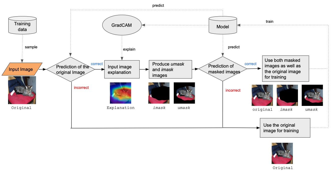
Figure 2: Explainer-driven data augmentation for multi-class image classification

Figure 2 shows the training process of EDDA in the multi-class classification setting. Let $\mathcal{M}$ denotes the training model, then in each epoch, for an input image $x\in\mathbb{R}^{w\times h\times c}$ with a predicted label $y=\mathcal{M}(x)$ and a ground truth label $\hat{y}$, we only perform augmentation when the prediction is correct, i.e. $y=\hat{y}$. Otherwise, we train the classifier with the original image alone.

If the prediction is correct, we then use the explainer $f_{\mathcal{M}}$ to obtain the saliency map $s_{x}^{y}$ indicating the attribution of each pixel to the prediction $y$:

$$s_{x}^{y}=f_{\mathcal{M}}(x,y)$$ (2)

where $s_{x}^{y}\in\mathbb{R}^{w\times h}$ and is normalized into the range of $[0,1]$.

Next, we generate two masked images. We generate the umask image $x_{umask}$ by preserving the pixels with saliency scores that are above a threshold $\tau_{umask}$ (a hyperparameter) and masking out other pixels:

$$x_{umask}=x\odot(s_{x}^{y}>\tau_{umask}),$$ (3)

where $x_{umask}\in\mathbb{R}^{w\times h\times c}$. Correspondingly, we generate imask image $x_{imask}$ by occluding the pixels with saliency scores above a threshold $\tau_{imask}$:

$$x_{imask}=x\odot(s_{x}^{y}<\tau_{imask}).$$ (4)

We obtain the prediction $\hat{y}_{umask}$ and $\hat{y}_{imask}$ on the perturbed images $x_{umask}$ and $x_{imask}$ by feeding them into the classifier $\mathcal{M}$.

If the imask image has the same prediction as the original image (i.e. $\hat{y}_{imask}=y$), meaning that the explanation may not be faithful and there is still discriminative information in the masked image, we then label the imask image as the original image’s prediction label $y$, and add the data $(x_{imask},y)$ into the current training batch. If the imask images has a different prediction than the one for the original image, we do not include the imask image for training.

Similarly, if the umask image has the same prediction as the original image (i.e. $\hat{y}_{umask}=y$), meaning that the explanation is faithful and the umask image preserves key information for classification, we then add the umask image with the image’s prediction label $(x_{umask},y)$ into the current training batch. Otherwise, we do not include the umask image in the training process. We summarize our proposed pipeline in Algorithm 2 in the appendix.

3.3 EDDA for Multi-label Classification

We propose a separate method in the multi-label classification setting, where there are multiple ground truth labels for a single image. This raises the needs for doing independent explanations with respect to different labels. We first make predictions on the input image, and then select the set of classes that have positive predictions and align with the ground truth labels - the True-Positive classes. We explain the input image with respect to each of these classes and generate the according imask images. For each imask image, if the prediction is correct on the according label, then we add that imask image with the original labels into the current training batch. The full algorithm is suggested in Algorithm 3.

4 Experiments and Evaluations

We perform a range of experiments with multiple datasets and models to evaluate the performance of EDDA against other methodologies. The experiment demonstrates the effectiveness of EDDA on the improvement of explanation faithfulness. We further investigate the visualization of masked images along the training process of EDDA and show that explanations are improved over time.

4.1 Experiment Settings

Datasets

We use CIFAR-100 [1] for multi-class classification and PASCAL VOC 2012 [32] for multi-label classification. Details about train and validation split and data pre-processing are stated in the appendix.

Models

To verify our consistent performance on different backbone models, we performed experiments on two popular convolution networks: ResNet-50 [2] and VGG-16 [3].

Hyperparameters

We tuned several method-based hyperparameters, including the threshold parameters $\tau_{imask}$ and $\tau_{umask}$in EDDA, as well as the Beta distribution parameter $\alpha$ in MixUp [34]. For fair comparison, we used the same training hyperparameters settings (e.g. batch size, number of epochs) in all methods. Details are in the appendix.

4.2 Experiment Methods

Baselines

For the purpose of thoroughly verifying the explanation capability of the EDDA method, we implemented the following non-explanation driven baselines as comparisons.

• No Augmentation: the vanilla training pipeline without any forms of data augmentation.

• CutMix [35]: it belongs to a type of regional dropout method, which randomly removes some image regions and fills them with patches from other training images. The target labels are assigned based on the proportion of the area of those patches.

• MixUp [34]: it does not use regional drop but linearly blends two training inputs instead. The targets of the augmented images are assigned based on the blending ratio of their source images.

• AugMix [36]: it creates several augmentations of every input and then linearly combine them with the original images by sampled weights. The targets remain unchanged. Similar to the original paper, we adopted the Jensen-Shannon Consistency Loss.

Our Methods

In terms of the explanation-driven data augmentation, we performed experiments under the EDDA framework with the following two explainers:

• Random Explainer (RandExp): it attributes a random saliency score to every pixel uniformly in the range of $[0,1]$. It is a trivial but important baseline.

• GradCAM (for EDDA): the explainer we chose to demonstrate EDDA’s capability. It uses the gradients of any target concept flowing into the final convolutional layer to produce a coarse localization map highlighting the important regions in the image for predicting the concept [23].

Evaluation Metrics

We applied the metrics of Drop% and Increase% introduced in [38, 39, 30] which can exactly demonstrate our claim. Drop% measures the positive attribution loss after a umask, while Increase% measures the negative attribution discard [30]. We adapted these two metrics, where for both Drop% and Increase% we measure the average magnitude of drop and increase of the confidence score with respect to the predicted label after occluding least salient regions, which is defined as

$$\begin{split}Drop\%=\frac{1}{N}\sum_{i=1}^{N}\frac{\mathrm{max}(0,\phi(x_{i})^{\hat{y_{i}}}-\phi(x_{i,umask})^{\hat{y_{i}}})}{\phi(x_{i})^{\hat{y_{i}}}}\times 100\\ Increase\%=\frac{1}{N}\sum_{i=1}^{N}\frac{\mathrm{max}(0,\phi(x_{i,umask})^{\hat{y_{i}}}-\phi(x_{i})^{\hat{y_{i}}})}{\phi(x_{i})^{\hat{y_{i}}}}\times 100\\ \end{split}$$ (5)

where $x_{i}$ represents the input image, $\mathcal{M}$ represents the classifier and returns a predicted label, $\phi(x_{i})^{\hat{y_{i}}}$ gives a confidence score of input $x_{i}$ with respect to $\hat{y_{i}}$, where $\hat{y_{i}}=\mathcal{M}(x_{i})$ is the predicted label.

In our experiments, we set the top 15% as the threshold (following previous work [30]) for selecting the most salient pixels for reservation. We also tried other thresholds including 30% and 50% and they displayed similar trends. If the explainer is faithful to the model, the umasked image should preserve the most discriminative regions [38], hence has a high confidence score which leads to a lower Drop% and a higher Increase%. These metrics do not require ground truth bounding boxes for the classified objects, which are expensive to label especially in real-world applications.

4.3 Performance Comparison on Explanation Faithfullness

Table 1: ResNet-50 and VGG-16 model performance in terms of Drop%_mag and Increase%_mag on CIFAR-100 and PASACL VOC 2012.

Model	ResNet-50		VGG-16
Metric	$Drop\%$ (Lower is better)	$Increase\%$ (Higher is better)	$Drop\%$ (Lower is better)	$Increase\%$ (Higher is better)
No Aug	$96.15\pm 0.30$	$0.35\pm 0.09$	$93.41\pm 0.52$	$0.25\pm 0.06$
CutMix	$96.38\pm 0.34$	$0.24\pm 0.02$	$95.09\pm 0.36$	$0.24\pm 0.04$
MixUp	$94.80\pm 0.47$	$0.62\pm 0.15$	$93.80\pm 0.33$	0.99 $\pm$ 0.23
AugMix	$95.86\pm 0.17$	$0.32\pm 0.03$	$94.29\pm 0.55$	$0.22\pm 0.06$
RandExp	$95.91\pm 0.31$	$0.39\pm 0.05$	$93.99\pm 0.57$	$0.33\pm 0.11$
EDDA	82.22 $\pm$ 0.30	1.32 $\pm$ 0.13	88.15 $\pm$ 0.60	$0.45\pm 0.12$

(a) CIFAR-100

Model	ResNet-50		VGG-16
Metric	$Drop\%$ (Lower is better)	$Increase\%$ (Higher is better)	$Drop\%$ (Lower is better)	$Increase\%$ (Higher is better)
No Aug	$53.84\pm 3.95$	$1.27\pm 0.42$	$40.71\pm 2.30$	$3.25\pm 0.84$
CutMix	$62.52\pm 4.90$	$1.84\pm 0.52$	$48.55\pm 2.34$	$1.85\pm 0.16$
MixUp	$55.67\pm 1.28$	$2.87\pm 0.43$	$46.83\pm 0.94$	$1.95\pm 0.17$
AugMix	$49.02\pm 3.21$	$1.91\pm 0.18$	$41.10\pm 1.97$	19.33 $\pm$ 13.54
RandExp	$75.39\pm 5.76$	$8.61\pm 4.27$	$45.28\pm 1.23$	$7.21\pm 4.12$
EDDA	42.72 $\pm$ 7.50	11.89 $\pm$ 14.57	9.01 $\pm$ 3.35	$9.00\pm 3.28$

(b) PASCAL VOC 2012

Table 1(b) shows the Drop% and the Increase% evaluation results on the CIFAR-100 dataset and the PASCAL VOC 2012 dataset with both ResNet-50 and VGG-16 models. We report the average scores and 95% confidence intervals over five independent runs with different random seeds.

It can be observed that EDDA has the best $Drop\%$ scores compared to all the baseline methodologies, especially with PASCAL VOC 2012 on VGG (30% lower than others) . For $Increase\%$, EDDA peforms the best across both datasets with the ResNet model. Whereas EDDA ranks second on $Increase\%$ of VGG-16 model for both datasets, it still performs better than four baselines.

To further understand the explainer behaviour with different augmentation techniques, we visualize the umask images in Figure 3. Here, we have the following observations:

• Quantitatively, $Drop\%$ scores of EDDA are significantly smaller than other methods.

• Qualitatively, EDDA generates umask images that correspond more closely to the prediction labels. For example, in the Person sample in Figure 3, the baselines generate umask images either containing parts of the car (No Aug, MixUp) or parts of the bicycle(CutMix, AugMix), whereas EDDA only shows regions of the person.

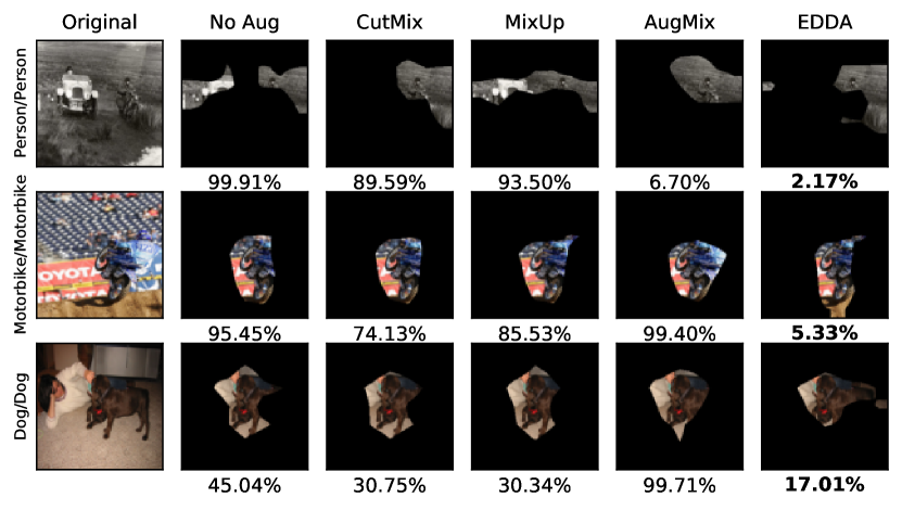
Figure 3: Sample test umask images generated with different augmentation methods from PASACL VOC 2012 dataset. The numbers below are the $Drop\%$ score and the title on the left is the target/prediction labels of each sample. All images are predicted correctly.

4.4 Explanation Improvement along the Training Process

To investigate the explanation faithfulness improvement of EDDA models along the growth of training iterations, we plot imask and umask images ($\tau_{imask}=\tau_{umask}=0.5$) generated at 4 model checkpoints (epoch 50, 100, 150 and 200) in Figure 4. Here, we make the following key observations:

• The predicted labels of the masked images change towards the desired direction along the training process. For the first example, the imask image is still predicted as the original label "Man" at epoch 50 and a similar label "Woman" at epoch 100. At epoch 150 and 200, the prediction changes to "Skyscraper" that is totally different from the original prediction. For the second example, along the training process, the prediction of imask images changes from a different label "Rabbit" to the original predicted label "Possum".

• Visually, the masked images identify the important/unimportant regions better along the process. Specifically, the imask images contain less information associated with the original label "Man" in later epochs, whereas the umask images contain more important information of "Possum" in later epochs.

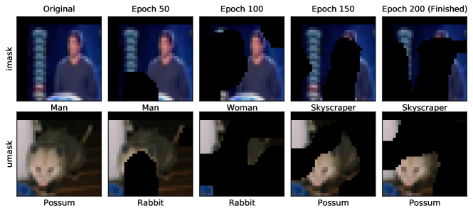
Figure 4: Sample imask and umask images generated at different epochs with EDDA from CIFAR-100 dataset on Resnet-50. The label below is the predicted label of each image

5 Conclusion

In this paper, we propose a novel explanation-driven data augmentation (EDDA) to improve the faithfulness of explanation methodologies with respect to the CNN model predictions. We verify our proposed method with two image datasets ( CIFAR-100 [1] and PASCAL VOC 2012 [32]) and two CNN ( ResNet [2] and VGG [3] ) models with GradCAM [23] as the explainer. Through these experiments, we empirically show that our method gives explanations that are more faithful to the model predictions across different datasets and CNN models both qualitatively and quantitatively compared to the non-explanation-driven augmentation methods and as well as no augmentation.

Appendix A Algorithms

This section contains the algorithms that we use in the main sections of the paper.

Input: train set $\mathcal{D}$, classifier $\mathcal{M}$, explainer $f_{\mathcal{M}}(\cdot)$, training epochs $E$, mini-batch size $N$

for $e\in\{1,...,E\}$ do

      

      for $(\mathcal{X},\mathcal{Y})\stackrel{{\scriptstyle N}}{{\sim}}\mathcal{D}$ do

            

            $\tilde{\mathcal{X}},\tilde{\mathcal{Y}}\leftarrow$ $\textbf{EDDA}(\mathcal{X},\mathcal{Y},\mathcal{M},f_{\mathcal{M}})$ $\triangleright$ use Algorithm 2 or Algorithm 3 depending on the task

            $\mathcal{M}\leftarrow\mathrm{Train(\mathcal{M},\tilde{\mathcal{X}},\tilde{\mathcal{Y}})}$

       end for

      

end for

Algorithm 1 Training Pipeline for Explanation-driven Data Augmentation

Input: input image batch $\mathcal{X}$, target label batch $\mathcal{Y}$, model $\mathcal{M}$, explainer $f_{\mathcal{M}}(\cdot)$, mini-batch size $N$

$\mathcal{X}^{\prime},\mathcal{Y}^{\prime}\leftarrow\{\},\{\}$

// Get the attribution map using explainer $f_{\mathcal{M}}$

$\mathcal{S}_{\mathcal{X}}^{\mathcal{Y}}\leftarrow f_{\mathcal{M}}(\mathcal{X},\mathcal{Y})$ $\triangleright$ Equation (2)

// Mask the most salient regions using a hyperparameter $\tau_{imask}$, where imask stands for important-mask

$\mathcal{X}_{imask}\leftarrow\mathcal{X}\odot(\mathcal{S}_{\mathcal{X}}^{\mathcal{Y}}>\tau_{imask})$ $\triangleright$ Equation (3)

// Mask the most unsalient regions using a hyperparameter $\tau_{umask}$, where umask stands for unimportant-mask

$\mathcal{X}_{umask}\leftarrow\mathcal{X}\odot(\mathcal{S}_{\mathcal{X}}^{\mathcal{Y}}<\tau_{umask})$ $\triangleright$ Equation (4)

// Predict the labels based on imasked and umasked images.

$\hat{\mathcal{Y}}_{imask}\leftarrow\mathcal{M}(\mathcal{X}_{imask})$

$\hat{\mathcal{Y}}_{umask}\leftarrow\mathcal{M}(\mathcal{X}_{umask})$

// Predict the labels based on original images.

$\hat{\mathcal{Y}}\leftarrow\mathcal{M}(\mathcal{X})$

for $1\leq k\leq N$ do

      

      if $\mathcal{Y}[k]=\hat{\mathcal{Y}}[k]$ then

             if $\mathcal{Y}[k]=\hat{\mathcal{Y}}_{imask}[k]$ then

                   // If the prediction on the imasked image aligns with the ground truth label, then

                   // concatenate the imasked image and the original label into the current training batch.

                   $\mathcal{X}^{\prime}\leftarrow\mathcal{X}^{\prime}\cup\{\mathcal{X}_{imask}[k]\}$

                   $\mathcal{Y}^{\prime}\leftarrow\mathcal{Y}^{\prime}\cup\{\mathcal{Y}[k]\}$

             end if

            

            if $\mathcal{Y}[k]=\hat{\mathcal{Y}}_{umask}[k]$ then

                   // If the prediction on the umasked image aligns with the ground truth label, then

                   // concatenate the umasked image and the original label into the current training

                   // batch.

                   $\mathcal{X}^{\prime}\leftarrow\mathcal{X}^{\prime}\cup\{\mathcal{X}_{umask}[k]\}$

                   $\mathcal{Y}^{\prime}\leftarrow\mathcal{Y}^{\prime}\cup\{\mathcal{Y}[k]\}$

             end if

            

       end if

      

end for

return $\mathcal{X}^{\prime}$, $\mathcal{Y}^{\prime}$

Algorithm 2 $\textbf{EDDA}_{mc}$: Explanation-driven Data Augmentation for Multi-class Classification

Input: input image batch $\mathcal{X}$, target label batch $\mathcal{Y}$, model $\mathcal{M}$, explainer $f_{\mathcal{M}}(\cdot)$

$\mathcal{X}^{\prime},\mathcal{Y}^{\prime}\leftarrow\mathcal{X},\mathcal{Y}$

for $1\leq k\leq|\mathcal{X}|$ do

       // Obtain the prediction given by the classifier.

       $\hat{\mathcal{Y}}\leftarrow\mathcal{M}(\mathcal{X}[k])$

       // Comparing with the ground truth labels, we select the True-Positive classes (where the

       // prediction and the label are both True) and denote the set to be $c$

       $\mathcal{C}\leftarrow indices(\hat{\mathcal{Y}}=\mathcal{Y}[k])$

      // Get the importance maps for all correct labels at the same time using explainer $f_{\mathcal{M}}$.

       $\mathcal{S}_{\mathcal{X}}^{\mathcal{Y}}\leftarrow f_{\mathcal{M}}(\mathcal{X}[k],\mathcal{C})$

      // Mask the most salient regions using a pre-defined hyperparameter $\tau$.

       $\mathcal{\mathcal{X}}_{imask}\leftarrow\mathcal{X}[k]\odot(\mathcal{S}_{\mathcal{X}}^{\mathcal{Y}}>\tau)$

      // Predict the labels based on masked images.

       $\hat{\mathcal{Y}}_{imask}\leftarrow\mathcal{M}(\mathcal{\mathcal{X}}_{imask})$

      for $1\leq z\leq\mathbf{|\mathcal{C}|}$ do

             if $\hat{\mathcal{Y}}_{imask}[z]=\mathcal{Y}[k,z]$ then

                   $\mathcal{X}^{\prime}\leftarrow\mathcal{X}^{\prime}\cup\{\mathcal{\mathcal{X}}_{imask}[z]\}$

                   $\mathcal{Y}^{\prime}\leftarrow\mathcal{Y}^{\prime}\cup\{\mathcal{Y}[k]\}$

                  

             end if

            

       end for

      

end for

return $\mathcal{X^{\prime}},\mathcal{Y^{\prime}}$

Algorithm 3 $\textbf{EDDA}_{ml}$: Explanation-driven Data Augmentation for Multi-label Classification

Appendix B Training Settings

Train, Validation & Test Set

For both CIFAR-100 dataset [1] and PASCAL VOC 2012 dataset [32], we randomly split out 20% of training data into the validation set, making the train v.s. validation ratio 4:1. We maintained the same ratio for the training of baselines and EDDA. The validation sets are used for model-related hyperparameter tuning and the evaluation are performed on the test set.

Data Pre-processing

To standardize the model inputs, we performed different kinds of data pre-processing on different datasets.

• CIFAR-100: We used standard image processing techniques such as cropping and flipping following the setting in [34, 35].

• PASCAL VOC 2012: Images were resized to 224*224 and no other pre-processing are done.

Hyperparameters

For fair comparisons, we used the same batch size, number of epochs, learning rate and weight decay for each Dataset & Model combination, regardless of which training methods were used. Table 2 includes all the non-model-related hyperparameters that we empirically chose.

Table 2: Hyperparameter settings of different Dataset & Model combinations

Dataset	CIFAR-100		PASCAL VOC 2012
Model	ResNet-50	VGG-16	ResNet-50	VGG-16
Batch Size	$512$	$512$	$8$	$8$
Number of Epochs	$200$	$200$	$20$	$20$
Learning Rate	$0.01$	$0.01$	$0.01$	$0.01$
Weight Decay	$0.0001$	$0.0001$	$0.0001$	$0.0001$

Additionally, in terms of MixUp [34] and AugMix [36] augmentation methods, we considered the effect of parameter $\alpha$ inside the Beta distribution in the set of 0.5, 1, as well as the Jensen-Shannon Consistency Loss respectively. From the validation results, we empirically found that $\alpha$ did not influence the performance a lot, therefore we chose the best $\alpha$ for each random seed. As for the Jensen-Shannon Consistency Loss, it was helpful with CIFAR-100 training but would harm the PASCAL VOC 2012 a lot, and we chose not to use it as a result.

Last but not least, we tuned the imask and umask thresholds $\tau_{imask}$,$\tau_{umask}$ and the epoch rate r when we got the explainer involved (Exp_epoch_rate) (e.g.: if the number of epochs is 200 and r is 0.5, then the first 100 epochs would do no augmentation, and the next 100 epochs would be EDDA training). We tuned $\tau_{imask}$,$\tau_{umask}$ in the set of $\{0.1,0.2,0.3,0.4,0.5\}$. We empirically set the ($\tau_{imask}$, $\tau_{umask}$) to be (0.5, 0.5) for ResNet-50 CIFAR-100 models, and (0.2, 0.2) for VGG-16 CIFAR-100 models. Since we only use imask for multi-label PASCAL VOC 2012 dataset, the $\tau_{imask}$ was empirically set to 0.5 for both ResNet-50 and VGG-16 models.

As for Exp_epoch_rate r, we empirically found that an r of 0.0 (i.e.: when the explainer was involved from the very beginning) led to the best Drop% and Increase%, while all Exp_epoch_rates shared similar accuracy. Therefore, 0.0 was the best r we had chosen.

Appendix C Additional Experimental Results

Apart from Drop% and Increase%, we also evaluated the EDDA models as well as the baseline models with Deletion_zero, Deletion_blur, Insertion_zero and Insertion_blur, following previous works on Deletion game and Insertion game based on the change in the confidence score [40]. We measured the AUC of confidence scores based on softmax probability after class logits and prediction accuracy when the image is gradually masked or recovered from mask. Regarding the type of masking, we have tried masking with blur and masking with zero (a black masking). The results of Deletion and Insertion of both types of masking are shown in Table 3(b) and Table 4(b). We have good Insertion results for both zero and blur masking, and we do not perform well in Deletion, which is within our expectation, as we are exactly training on the masked images, improving the robustness on partial image prediction and hence resulting in a high confidence score even on masked images.

Table 3: ResNet-50 and VGG-16 model performance in terms of Deletion_zero-score and Insertion_zero-score on CIFAR-100 and PASACL VOC 2012.

Model	ResNet-50		VGG-16
Metric	Deletionzero-score	Insertionzero-score	Deletionzero-score	Insertionzero-score
No Aug	$22.36\pm 0.50$	$27.30\pm 0.41$	22.58 $\pm$ 0.40	$36.30\pm 0.61$
CutMix	$19.83\pm 0.51$	$25.91\pm 0.55$	$25.76\pm 0.71$	$29.84\pm 0.95$
MixUp	17.53 $\pm$ 0.43	$20.32\pm 0.44$	$22.71\pm 0.65$	$24.66\pm 0.75$
AugMix	$23.17\pm 0.31$	$28.20\pm 0.18$	$23.47\pm 0.76$	$37.08\pm 0.73$
RandExp	$22.78\pm 0.24$	$26.76\pm 0.40$	$26.57\pm 0.55$	$34.54\pm 0.58$
EDDAGC	$39.77\pm 0.50$	46.08 $\pm$ 0.38	$42.52\pm 0.80$	53.34 $\pm$ 0.32

(a) CIFAR-100

Model	ResNet-50		VGG-16
Metric	Deletionzero-score	Insertionzero-score	Deletionzero-score	Insertionzero-score
No Aug	$27.16\pm 1.16$	$78.25\pm 1.33$	$23.01\pm 0.89$	$77.53\pm 1.08$
CutMix	$31.86\pm 1.14$	$69.17\pm 1.50$	$27.36\pm 0.59$	$66.56\pm 0.99$
MixUp	$29.82\pm 1.01$	$71.67\pm 1.15$	$23.39\pm 0.28$	$67.06\pm 0.53$
AugMix	$26.15\pm 1.15$	$74.08\pm 1.21$	19.69 $\pm$ 0.97	$77.08\pm 0.95$
RandExp	21.58 $\pm$ 2.25	$63.52\pm 3.79$	$23.25\pm 0.93$	$75.04\pm 0.80$
EDDAGC	$34.44\pm 4.41$	79.45 $\pm$ 3.23	$48.23\pm 2.25$	92.06 $\pm$ 2.01

(b) PASCAL VOC 2012

Table 4: ResNet-50 and VGG-16 model performance in terms of Deletion_blur-score and Insertion_blur-score on CIFAR-100 and PASACL VOC 2012.

Model	ResNet-50		VGG-16
Metric	Deletionblur-score	Insertionblur-score	Deletionblur-score	Insertionblur-score
No Aug	$32.63\pm 0.67$	$39.64\pm 0.31$	$31.17\pm 0.45$	$45.60\pm 0.64$
CutMix	$27.89\pm 0.67$	$36.37\pm 0.74$	$33.83\pm 0.94$	$39.47\pm 1.01$
MixUp	25.80 $\pm$ 0.83	$29.55\pm 0.98$	28.98 $\pm$ 0.71	$31.76\pm 0.97$
AugMix	$34.27\pm 0.36$	$40.35\pm 0.29$	$32.55\pm 0.46$	$45.66\pm 0.91$
RandExp	$36.24\pm 0.86$	$42.24\pm 0.68$	$36.75\pm 0.64$	$45.10\pm 0.75$
EDDAGC	$40.28\pm 0.66$	47.32 $\pm$ 0.49	$38.51\pm 1.03$	48.85 $\pm$ 0.52

(a) CIFAR-100

Model	ResNet-50		VGG-16
Metric	Deletionblur-score	Insertionblur-score	Deletionblur-score	Insertionblur-score
No Aug	$56.03\pm 1.14$	89.89 $\pm$ 0.30	$38.90\pm 0.64$	$90.98\pm 0.23$
CutMix	$53.73\pm 1.93$	$81.06\pm 1.08$	$39.84\pm 0.43$	$80.10\pm 0.24$
MixUp	$49.14\pm 0.86$	$82.18\pm 0.80$	$36.23\pm 0.45$	$81.15\pm 0.45$
AugMix	$60.17\pm 1.54$	$85.93\pm 0.53$	31.66 $\pm$ 0.62	$91.57\pm 0.27$
RandExp	$43.68\pm 6.51$	$78.76\pm 3.96$	$45.31\pm 0.89$	93.22 $\pm$ 0.41
EDDAGC	38.53 $\pm$ 2.11	$82.81\pm 2.92$	$44.02\pm 1.19$	$91.64\pm 0.89$

(b) PASCAL VOC 2012

Appendix D Criticisms and Limitations

Table 5: Test accuracy of ResNet-50, VGG-16 on CIFAR-100 and PASCAL VOC 2012.

Dataset	CIFAR-100		PASCAL VOC 2012
Model	ResNet-50	VGG-16	ResNet-50	VGG-16
No Aug	$63.33\pm 0.21$	$69.65\pm 0.38$	77.51 $\pm$ 0.26	$73.95\pm 0.26$
CutMix	67.22 $\pm$ 0.42	73.43 $\pm$ 0.20	$76.09\pm 0.61$	$72.12\pm 0.22$
MixUp	$65.88\pm 0.24$	$71.80\pm 0.47$	$75.82\pm 0.35$	$72.56\pm 0.40$
AugMix	$62.24\pm 0.47$	$69.44\pm 0.22$	$76.46\pm 0.40$	$73.99\pm 0.19$
RandExp	$57.28\pm 0.40$	$66.74\pm 0.48$	$70.44\pm 2.13$	$72.72\pm 0.23$
EDDA	$61.21\pm 0.34$	$69.43\pm 0.35$	$69.42\pm 1.72$	74.69 $\pm$ 0.52

As shown in Table 5, the EDDA models does not have great accuracy performance. If a model has simple structure, it would be easy to explain but it’s accuracy may be sacrificed due to its simplicity. In contrast, the accuracy of a complex model can be high, but it may lead to low explanation results [41]. From another perspective, the EDDA method is designed primarily to improve the explanation faithfulness, therefore it is reasonable to result in an acceptable degree of drop in accuracy, as there could be trade-offs between model and explanation faithfulness and accuracy.

Another limitation is the lack of appropriate baselines. To the best of our knowledge, there are no explanation-driven data augmentation methods that are also targeting to improving explanation faithfulness in the training pipeline. As a result, we could only compare with non-explanation-driven data augmentation methods and the trivial Random Explainer baseline.

References

- [1] Alex Krizhevsky, Geoffrey Hinton, et al. Learning multiple layers of features from tiny images. 2009.
- [2] Kaiming He, Xiangyu Zhang, Shaoqing Ren, and Jian Sun. Deep residual learning for image recognition. In Proceedings of the IEEE conference on computer vision and pattern recognition, pages 770–778, 2016.
- [3] Karen Simonyan and Andrew Zisserman. Very deep convolutional networks for large-scale image recognition. arXiv preprint arXiv:1409.1556, 2014.
- [4] Joseph Redmon, Santosh Divvala, Ross Girshick, and Ali Farhadi. You only look once: Unified, real-time object detection. In Proceedings of the IEEE Conference on Computer Vision and Pattern Recognition (CVPR), June 2016.
- [5] Shaoqing Ren, Kaiming He, Ross Girshick, and Jian Sun. Faster r-cnn: Towards real-time object detection with region proposal networks. In C. Cortes, N. Lawrence, D. Lee, M. Sugiyama, and R. Garnett, editors, Advances in Neural Information Processing Systems, volume 28. Curran Associates, Inc., 2015.
- [6] Jonathan Long, Evan Shelhamer, and Trevor Darrell. Fully convolutional networks for semantic segmentation, 2014.
- [7] Olaf Ronneberger, Philipp Fischer, and Thomas Brox. U-net: Convolutional networks for biomedical image segmentation, 2015.
- [8] Liang-Chieh Chen, George Papandreou, Iasonas Kokkinos, Kevin Murphy, and Alan L. Yuille. Deeplab: Semantic image segmentation with deep convolutional nets, atrous convolution, and fully connected crfs, 2016.
- [9] Andre Esteva, Alexandre Robicquet, Bharath Ramsundar, Volodymyr Kuleshov, Mark DePristo, Katherine Chou, Claire Cui, Greg Corrado, Sebastian Thrun, and Jeff Dean. A guide to deep learning in healthcare. Nature medicine, 25(1):24–29, 2019.
- [10] Aditya Chattopadhay, Anirban Sarkar, Prantik Howlader, and Vineeth N Balasubramanian. Grad-cam++: Generalized gradient-based visual explanations for deep convolutional networks. In 2018 IEEE Winter Conference on Applications of Computer Vision (WACV), pages 839–847. IEEE, 2018.
- [11] Ian Covert, Scott Lundberg, and Su-In Lee. Understanding global feature contributions with additive importance measures. Advances in Neural Information Processing Systems, 33, 2020.
- [12] Eunsuk Chong, Chulwoo Han, and Frank C Park. Deep learning networks for stock market analysis and prediction: Methodology, data representations, and case studies. Expert Systems with Applications, 83:187–205, 2017.
- [13] Yash Goyal, Ziyan Wu, Jan Ernst, Dhruv Batra, Devi Parikh, and Stefan Lee. Counterfactual visual explanations. In International Conference on Machine Learning, pages 2376–2384. PMLR, 2019.
- [14] Daniel Smilkov, Nikhil Thorat, Been Kim, Fernanda Viégas, and Martin Wattenberg. Smoothgrad: removing noise by adding noise. arXiv preprint arXiv:1706.03825, 2017.
- [15] Mukund Sundararajan, Ankur Taly, and Qiqi Yan. Axiomatic attribution for deep networks. In International Conference on Machine Learning, pages 3319–3328. PMLR, 2017.
- [16] Scott Lundberg and Su-In Lee. A unified approach to interpreting model predictions. arXiv preprint arXiv:1705.07874, 2017.
- [17] Marco Tulio Ribeiro, Sameer Singh, and Carlos Guestrin. " why should i trust you?" explaining the predictions of any classifier. In Proceedings of the 22nd ACM SIGKDD international conference on knowledge discovery and data mining, pages 1135–1144, 2016.
- [18] Karen Simonyan, Andrea Vedaldi, and Andrew Zisserman. Deep inside convolutional networks: Visualising image classification models and saliency maps. arXiv preprint arXiv:1312.6034, 2013.
- [19] Terrance DeVries and Graham W Taylor. Improved regularization of convolutional neural networks with cutout. arXiv preprint arXiv:1708.04552, 2017.
- [20] Garima Pruthi, Frederick Liu, Satyen Kale, and Mukund Sundararajan. Estimating training data influence by tracing gradient descent. Advances in Neural Information Processing Systems, 33, 2020.
- [21] Pang Wei Koh and Percy Liang. Understanding black-box predictions via influence functions. In International Conference on Machine Learning, pages 1885–1894. PMLR, 2017.
- [22] Chih-Kuan Yeh, Joon Sik Kim, Ian EH Yen, and Pradeep Ravikumar. Representer point selection for explaining deep neural networks. arXiv preprint arXiv:1811.09720, 2018.
- [23] Ramprasaath R Selvaraju, Michael Cogswell, Abhishek Das, Ramakrishna Vedantam, Devi Parikh, and Dhruv Batra. Grad-cam: Visual explanations from deep networks via gradient-based localization. In Proceedings of the IEEE international conference on computer vision, pages 618–626, 2017.
- [24] David Alvarez-Melis and Tommi S. Jaakkola. On the robustness of interpretability methods, 2018.
- [25] Amirata Ghorbani, Abubakar Abid, and James Zou. Interpretation of neural networks is fragile. Proceedings of the AAAI Conference on Artificial Intelligence, 33(01):3681–3688, Jul. 2019.
- [26] Chih-Kuan Yeh, Cheng-Yu Hsieh, Arun Sai Suggala, David I Inouye, and Pradeep Ravikumar. On the (in) fidelity and sensitivity for explanations. arXiv preprint arXiv:1901.09392, 2019.
- [27] Jacob Sippy, Gagan Bansal, and Daniel S Weld. Data staining: A method for comparing faithfulness of explainers. In Proc. of ICML Workshop on Human Interpretability in Machine Learning (WHI), 2020.
- [28] Alon Jacovi and Yoav Goldberg. Towards faithfully interpretable nlp systems: How should we define and evaluate faithfulness? arXiv preprint arXiv:2004.03685, 2020.
- [29] Himabindu Lakkaraju, Ece Kamar, Rich Caruana, and Jure Leskovec. Faithful and customizable explanations of black box models. In Proceedings of the 2019 AAAI/ACM Conference on AI, Ethics, and Society, pages 131–138, 2019.
- [30] Sam Sattarzadeh, Mahesh Sudhakar, Anthony Lem, Shervin Mehryar, KN Plataniotis, Jongseong Jang, Hyunwoo Kim, Yeonjeong Jeong, Sangmin Lee, and Kyunghoon Bae. Explaining convolutional neural networks through attribution-based input sampling and block-wise feature aggregation. arXiv preprint arXiv:2010.00672, 2020.
- [31] Jay DeYoung, Sarthak Jain, Nazneen Fatema Rajani, Eric Lehman, Caiming Xiong, Richard Socher, and Byron C Wallace. Eraser: A benchmark to evaluate rationalized nlp models. arXiv preprint arXiv:1911.03429, 2019.
- [32] M. Everingham, L. Van Gool, C. K. I. Williams, J. Winn, and A. Zisserman. The PASCAL Visual Object Classes Challenge 2012 (VOC2012) Results. http://www.pascal-network.org/challenges/VOC/voc2012/workshop/index.html.
- [33] Bolei Zhou, Aditya Khosla, Agata Lapedriza, Aude Oliva, and Antonio Torralba. Learning deep features for discriminative localization. In Proceedings of the IEEE conference on computer vision and pattern recognition, pages 2921–2929, 2016.
- [34] Hongyi Zhang, Moustapha Cisse, Yann N Dauphin, and David Lopez-Paz. mixup: Beyond empirical risk minimization. arXiv preprint arXiv:1710.09412, 2017.
- [35] Sangdoo Yun, Dongyoon Han, Seong Joon Oh, Sanghyuk Chun, Junsuk Choe, and Youngjoon Yoo. Cutmix: Regularization strategy to train strong classifiers with localizable features. In Proceedings of the IEEE/CVF International Conference on Computer Vision, pages 6023–6032, 2019.
- [36] Dan Hendrycks, Norman Mu, Ekin D. Cubuk, Barret Zoph, Justin Gilmer, and Balaji Lakshminarayanan. AugMix: A simple data processing method to improve robustness and uncertainty. Proceedings of the International Conference on Learning Representations (ICLR), 2020.
- [37] Riccardo Guidotti, Anna Monreale, Salvatore Ruggieri, Franco Turini, Fosca Giannotti, and Dino Pedreschi. A survey of methods for explaining black box models. ACM Comput. Surv., August 2018.
- [38] Harish Guruprasad Ramaswamy et al. Ablation-cam: Visual explanations for deep convolutional network via gradient-free localization. In Proceedings of the IEEE/CVF Winter Conference on Applications of Computer Vision, pages 983–991, 2020.
- [39] Ruigang Fu, Qingyong Hu, Xiaohu Dong, Yulan Guo, Yinghui Gao, and Biao Li. Axiom-based grad-cam: Towards accurate visualization and explanation of cnns. arXiv preprint arXiv:2008.02312, 2020.
- [40] Vitali Petsiuk, Abir Das, and Kate Saenko. Rise: Randomized input sampling for explanation of black-box models. arXiv preprint arXiv:1806.07421, 2018.
- [41] W. James Murdoch, Chandan Singh, Karl Kumbier, Reza Abbasi-Asl, and Bin-Xia Yu. Interpretable machine learning: definitions, methods, and applications. ArXiv, abs/1901.04592, 2019.