Minimizing Oracle-Structured Composite Functions

Abstract

We consider the problem of minimizing a composite convex function with two different access methods: an oracle, for which we can evaluate the value and gradient, and a structured function, which we access only by solving a convex optimization problem. We are motivated by two associated technological developments. For the oracle, systems like PyTorch or TensorFlow can automatically and efficiently compute gradients, given a computation graph description. For the structured function, systems like CVXPY accept a high level domain specific language description of the problem, and automatically translate it to a standard form for efficient solution. We develop a method that makes minimal assumptions about the two functions, does not require the tuning of algorithm parameters, and works well in practice across a variety of problems. Our algorithm combines a number of well-known ideas, including a low-rank quasi-Newton approximation of curvature, piecewise affine lower bounds from bundle-type methods, and two types of damping to ensure stability. We illustrate the method on stochastic optimization, utility maximization, and risk-averse programming problems, showing that our method is more efficient than standard solvers when the oracle function contains much data.

1 Introduction

Our story starts with a well studied problem, minimizing a convex function that is the sum of two convex functions with different access methods, referred to as a composite function nesterov2013gradient . The first function is smooth, and we can access it only by a few methods, such as evaluating its value and gradient at a given point. The other function is not necessarily smooth, but is structured, and we can access it only by solving a convex optimization problem that involves it. In the typical setting, the second function is one for which we can efficiently compute its proximal operator, usually analytically. Here we assume a bit more for the second function, specifically, that we can minimize it plus a structured function of modest complexity.

Our goal is to minimize such functions automatically, with a method that works well across a large variety of problem instances using its default parameters. We leverage new technological developments: systems for automatic differentiation that automatically and effficiently compute gradients given a computation graph description, and systems for solving convex optimization problems described in a domain specific language for multiple parameter values.

1.1 Oracle-structured composite function

We seek to minimize $h(x)=f(x)+g(x)$ over $x\in{\mbox{\bf R}}^{n}$. We assume that

• $f:\Omega\to{\mbox{\bf R}}$ is convex and differentiable, where $\Omega\subseteq{\mbox{\bf R}}^{n}$ is convex and open. We assume that a point $x^{0}\in\Omega$ is known.

• $g:{\mbox{\bf R}}^{n}\to{\mbox{\bf R}}\cup\{+\infty\}$ is convex, with closed sublevel sets, and not necessarily differentiable. Infinite values of $g$ encode constraints on $x$.

Our method will access these two functions in very specific ways.

• We can evaluate $f(x)$ and $\nabla f(x)$ at any $x$. For $x\not\in\Omega$, our oracle returns the value $+\infty$ for $f(x)$. (We will discuss a few other possible access methods for $f$ in the sequel.)

• We can minimize $g(x)$ plus another structured function. Here we use the term structured loosely, to mean in the sense of Nesterov, or as a practical matter, in a disciplined convex programming (DCP) description. This is an extension of the usual assumption in composite function minimization that the proximal operator of $g$ can be evaluated analytically.

We refer to $f$ as the oracle part of the objective, $g$ as the structured part of the objective, and $h=f+g$ as an oracle-structured composite objective. We denote the optimal value of the problem as

$$h^{\star}=\inf_{x}\left(f(x)+g(x)\right).$$

Assumptions.

We assume that the sublevel sets of $h$ are compact, and $h^{\star}<\infty$ (so at least some sublevel sets are nonempty). These assumptions imply that $f(x)+g(x)$ has a minimizer, i.e., a point $x^{\star}$ with $h(x^{\star})=h^{\star}$. Our convergence proofs make the typical assumption that $\nabla f$ is Lipschitz continuous with constant $L$, but we stress that this is not used in the algorithm itself.

Optimality condition.

The optimality condition is

$$\nabla f(x)+q=0,\qquad q\in\partial g(x),$$ (1)

where $\partial g(x)$ denotes the subdifferential of $g$ at $x$. For $x\in\Omega$ and $q\in\partial g(x)$, we can interpret $\nabla f(x)+q$ as a residual in the optimality condition. (We will use this in the stopping criterion of our algorithm.) Our access to $f$ directly gives us $\nabla f(x)$; we will see that our access method to $g$ indirectly produces a subgradient $q\in\partial g(x)$.

1.2 Practical considerations

We are motivated by two technological considerations related to our access methods to $f$ and $g$, which we mention briefly here.

Handling $f$.

To handle $f$ we can rely on automatic differentiation systems that have been developed in recent years, such as PyTorch NEURIPS2019_9015 , TensorFlow tensorflow2015-whitepaper , and Zygote/Flux/Autograd maclaurin2015autograd ; Flux.jl-2018 ; innes2019differentiable . Automatic differentiation is an old topic nolan1953analytical ; adamson1969slang (see baydin2018automatic for a recent review), but these recent systems go way beyond the basic algorithms for automatic differentiation, in terms of ease of use and run-time efficiency, across multiple computation platforms. We describe $f$ (but not its gradient) using existing libraries and languages; thereafter, $f(x)$ and $\nabla f(x)$ can be evaluated very efficiently, on many computation platforms, ranging from single CPU to multiple GPUs. These systems are widely used throughout machine learning, mostly for fitting deep neural networks.

Handling $g$.

To handle $g$ we make use of domain specific languages (DSLs) for convex optimization, such as CVX grant2014cvx , CVXPY cvxpy_paper ; agrawal2018rewriting , and Convex.jl cvxjl . These systems take a description of $g$ in a special language based on disciplined convex programming (DCP) GBY:06 . This description of $g$ is then automatically transformed into a standard form, such as a cone program, and then solved. Recently, such systems have been enhanced to include parameters, which are constants in the problem each time it is solved, but can be changed and the problem re-solved efficiently, skipping the compilation process. These systems are reasonably good at preserving structure in the problem during compilation, so the solve times can be quite small when exploitable structure is present, which we will see is the case in our method.

We mention that $g$ can contain hidden additional variables. By this we mean that $g$ has the form $g(x)=\inf_{z}G(x,z)$, where $G$ is convex in $(x,z)$. Roughly speaking, $z$ is the hidden variable that does not appear in $f$. Such functions are immediately handled by structured systems, without any additional effort. In particular, we do not need to work out an analytical form for $g(x)$. In this case just evaluating $g$ requires solving an optimization problem (over $z$). Our method will avoid any evaluations of $g$.

When to just use a structured solver.

Finally, we mention that if $f$ is simple enough to be handled by a DCP-based system, then simply minimizing $f+g$ using such a system is the preferred method of solution. We are interested here in problems where this is not the case. Typically this means that $f$ is complex in the sense of involving substantial data, for example, a sample average of some function with $10^{6}$ or more samples. (We will see this phenomenon in the numerical examples given in §5.)

Contribution.

The method we propose in the next section is in the family of variable metric bundle methods, and closely related to a number of other methods found in the literature (we review related work in §2.9). As an algorithm, our method is not particularly novel; we consider our contribution to be its careful design to be compatible with our access methods, and the efficiency of the method compared with standard solvers when the function $f$ contains a large amount of data.

2 Oracle-structured minimization method

In this section we propose a generic method for solving the oracle-structured minimization problem, which we call oracle-structured minimization method (OSMM). OSMM combines several well known methods from optimization, including variable metric or quasi-Newton curvature estimates to accelerate convergence, bundle methods that build up a piecewise affine model, and two types of damping, based on a trust penalty and a line search. These are chosen to be compatible with our access methods.

We will denote the iterates with a superscript, so $x^{k}$ denotes the $k$th iterate of the algorithm. We will let $x^{k+1/2}$ denote the tentative iterate at the $(k+1)$st iteration, before the line search. We will assume that $x^{0}\in\Omega$, i.e., $f(x^{0})<\infty$. Our algorithm will guarantee that $x^{k}\in\Omega$ for all $k$. It is a descent method, i.e., $h(x^{k+1})<h(x^{k})$. While $h(x^{0})=\infty$ is possible, we will see that $h(x^{k})<\infty$ for $k\geq 1$.

As with many other optimization algorithms, OSMM is based on forming an approximation of the function $f$ in each iteration.

2.1 Approximation of the oracle function

In iteration $k$, we form a convex approximation of $f$, given by $\hat{f}_{k}:{\mbox{\bf R}}^{n}\to{\mbox{\bf R}}\cup\{\infty\}$, based on information obtained from previous iterations and possibly prior knowledge of $f$. The approximation has the specific form

$$\hat{f}_{k}(x)=l_{k}(x)+(1/2)(x-x^{k})^{T}H_{k}(x-x^{k}).$$ (2)

Here $H_{k}$ is positive semidefinite, and $l_{k}:{\mbox{\bf R}}^{n}\to{\mbox{\bf R}}\cup\{\infty\}$ is a convex minorant of $f$, i.e., $l_{k}(x)\leq f(x)$ for all $x$.

Assumptions on $H_{k}$.

The only assumption we make about $H_{k}$ is that it is positive semidefinite and bounded, i.e., there exists a $C$ such that $\|H_{k}\|_{2}\leq C$ for all $k$. In practice, $H_{k}$ accelerates convergence by serving as an estimate of the curvature of $f$. The simplest choice, $H_{k}=0$, results in an algorithm that converges but does not offer the practical benefit of convergence acceleration.

Choice of $H_{k}$.

There are many ways of choosing a positive semi-definite $H_{k}$ to approximate the curvature of $f$ at $x^{k}$. One obvious choice is the Hessian $H_{k}=\nabla^{2}f(x^{k})$, but this requires that $f$ be twice differentiable, and also violates our assumption about how we access $f$. A lesser violation of the access method might use an approximation of the Hessian based on evaluations of the mapping $z\mapsto\nabla^{2}f(x^{k})z$ (i.e., Hessian-vector multiplication), which can be practical in many cases erdogdu2015convergence . A simple and effective choice is $H_{k}=(a_{k}/n)I$, where $a_{k}$ is an approximation of $\mathop{\bf Tr}\nabla^{2}f(x^{k})$, obtained for example by the Hutchinson method hutchinson1989stochastic ; meyer2021hutch++ .

Quasi-Newton methods are a general class of curvature approximations that are compatible with our assumptions on the access method for $f$. These methods, which have a very long history, build up an approximation of $H_{k}$ using only the current and previously evaluated gradients davidon1959variable ; fletcher1963rapidly ; broyden1965class ; dennis1977quasi ; byrd1994representations . When $H_{k}$ is low rank, or diagonal plus low rank, the method is practical even for large values of $n$. (Such methods are often called limited memory, since they do not require the storage of an $n\times n$ matrix.) For OSMM we propose to use the low-rank quasi-Newton choice given in fletcher2005new , described in detail in §A.1. We can express $H_{k}$ as

$$H_{k}=G_{k}G_{k}^{T},$$ (3)

where $G_{k}\in{\mbox{\bf R}}^{n\times r}$, and $r$ is a chosen (maximum) rank for $H_{k}$.

As many others have observed, limited memory quasi-Newton methods deliver most of their benefit for relatively small values of $r$, like $r=10$ or $r=20$. These values allow the methods to be used even when $n$ is very large (say, $10^{5}$), since the storage requirement (specifically, of $G_{k}$) grows linearly with $r$, and the computational cost of evaluating $x^{k+1/2}$ grows quadratically in $r$, and only linearly in $n$.

Assumptions on $l_{k}$.

We make the usual assumption on the minorant $l_{k}$ that it is tight at $x^{k}$, i.e., $l_{k}(x^{k})=f(x^{k})$. It follows that $\hat{f}_{k}(x^{k})=f(x^{k})$. It also follows that $l_{k}$ is differentiable at $x^{k}$, and $\nabla l_{k}(x^{k})=\nabla f(x^{k})$. To see this, we note that since $l_{k}$ is a minorant of $f$, tight at $x^{k}$, we have

$$\partial l_{k}(x^{k})\subseteq\partial f(x^{k})=\{\nabla f(x^{k})\}.$$

The first inclusion can be seen since any affine lower bound on $l_{k}$, tight at $x^{k}$, is also an affine lower bound on $f$, tight at $x^{k}$, so its linear part is a subgradient of $f$ at $x^{k}$. The right-hand equality holds since $f$ is differentiable, so its subdifferential contains only one element, its gradient. Finally, since $\partial l_{k}(x^{k})$ contains only $\nabla f(x^{k})$, we conclude it is differentiable at $x^{k}$, with gradient $\nabla f(x^{k})$.

In addition to the mathematical assumptions about $l_{k}$ described above, we will assume that $l_{k}$ has a structured description. This implies that $\hat{f}_{k}$ has a structured description.

Minorants.

The simplest minorant is the first order Taylor approximation

$$l_{k}(x)=f(x^{k})+\nabla f(x^{k})^{T}(x-x^{k}).$$

A more complex minorant is the piecewise affine minorant

$$l_{k}(x)=\max_{i=1,\ldots,k}\left(f(x^{i})+\nabla f(x^{i})^{T}(x-x^{i})\right),$$

which uses all previously evaluated gradients of $f$.

For OSMM we propose the piecewise affine minorant

$$l_{k}(x)=\max_{i=\max\{0,k-M+1\},\ldots,k}\left(f(x^{i})+\nabla f(x^{i})^{T}(x-x^{i})\right),$$ (4)

the pointwise maximum of the affine minorants from the previous $M$ gradient evaluations, where $M$ is the memory. With memory $M=1$, this reduces to the Taylor approximation.

The problem of choosing the memory $M$ is very similar to the problem of choosing $r$, the rank of the curvature approximation. The storage requirements grows linearly with $M$, and the computational cost of evaluating $x^{k+1/2}$ grows quadratically with $M$. As with the choice of $r$, small values such as $M=10$ or $M=20$ seem to work well in practice.

We mention a few additional useful minorants that use additional prior information about $f$ or its domain $\Omega$. First, we can add to $l_{k}$ constraints that contain $\Omega$. Suppose we know that $\tilde{\Omega}\supset\Omega$, where $\tilde{\Omega}$ has a structured description, e.g., a box. We can then use the minorant

$$l_{k}(x)=\max_{i=\max\{0,k-M+1\},\ldots,k}\left(f(x^{i})+\nabla f(x^{i})^{T}(x-x^{i})\right)+I_{\tilde{\Omega}}(x),$$

where $I_{\tilde{\Omega}}$ is the indicator function of $\tilde{\Omega}$. In a similar way, if a (constant) lower bound $\ell$ on $f$ is known, we can replace any minorant $l_{k}$ with $\max\{l_{k}(x),\ell\}$.

If it is known that $f$ is $\rho$-strongly convex, we can strengthen the piecewise affine minorant (4) to the piecewise quadratic minorant

$$l_{k}(x)=\max_{i=\max\{0,k-M+1\},\ldots,k}\left(f(x^{i})+\nabla f(x^{i})^{T}(x-x^{i})+(\rho/2)\|x-x^{i}\|_{2}^{2}\right).$$

(Each term in the maximum has the same quadratic part $(\rho/2)\|x\|_{2}^{2}$, so $l_{k}$ can be expressed as a piecewise affine function plus $(\rho/2)\|x\|_{2}^{2}$.)

Lower bound.

We observe that

$$\ell_{k}=\inf_{x}\left(l_{k}(x)+g(x)\right)$$

is a lower bound on the optimal value $h^{\star}$. It can be computed using a system for structured optimization. At iteration $k$ we let $L_{k}$ denote the best (largest) lower bound found so far,

$$L_{k}=\max\{\ell_{1},\ldots,\ell_{k}\}.$$ (5)

2.2 Tentative update

At iteration $k$, our tentative next iterate $x^{k+1/2}$ is obtained by minimizing our approximation of $f$, plus $g$ and a trust penalty term:

$$x^{k+1/2}=\mathop{\rm argmin}_{x}\left(\hat{f}_{k}(x)+g(x)+\frac{\lambda_{k}}{2}\|x-x^{k}\|_{2}^{2}\right).$$ (6)

The last term is a (Levenberg-Marquardt or proximal) trust penalty, which penalizes deviation from $x^{k}$; the positive parameter $\lambda_{k}$ scales the trust penalty. We assume that $x^{k+1/2}$ in (6) can be computed using a system for structured optimization. (The minimizer in (6) exists and is unique, so $x^{k+1/2}$ is well defined. To see this we observe that the objective is finite for $x=x^{k}$, and the function being minimized is strictly convex.) We note that while $\hat{f}_{k}(x^{k+1/2})$ and $g(x^{k+1/2})$ are finite, $f(x^{k+1/2})=\infty$ (and therefore also $h(x^{k+1/2})=\infty$) is possible.

The two quadratic terms in the objective in (6) can be combined to express the tentative update as

$$x^{k+1/2}=\mathop{\rm argmin}_{x}\left(l_{k}(x)+g(x)+\frac{1}{2}(x-x^{k})^{T}(H_{k}+\lambda_{k}I)(x-x^{k})\right),$$ (7)

which shows that the trust penalty term can be interpreted as a regularizer for the curvature estimate $H_{k}$.

In the DCP description of the problem (7), using (3) we express the last term as

$$\frac{1}{2}(x-x^{k})^{T}(H_{k}+\lambda_{k}I)(x-x^{k})=\frac{1}{2}\|G_{k}^{T}(x-x^{k})\|_{2}^{2}+\frac{\lambda_{k}}{2}\|x-x^{k}\|_{2}^{2}.$$

This keeps the problem (7) tractable when $r\ll n$ and $n$ is large. In particular, there is no need to form the $n\times n$ matrix $H_{k}$.

Tentative update optimality condition.

For future reference, we note that the optimality condition for the minimization in (7) that defines $x^{k+1/2}$ is

$$0\in\partial l_{k}(x^{k+1/2})+\partial g(x^{k+1/2})+(H_{k}+\lambda_{k}I)(x^{k+1/2}-x^{k}).$$ (8)

When $l_{k}$ is the piecewise affine minorant (4), its subdifferential $\partial l_{k}(x^{k+1/2})$ has the form

$$\partial l_{k}(x^{k+1/2})={\mathop{\bf Co}}\{\nabla f(x^{i})\mid l_{k}(x^{k+1/2})=f(x^{i})+\nabla f(x^{i})^{T}(x^{k+1/2}-x^{i})\},$$ (9)

the convex hull of the gradients associated with the active terms in maximum defining $l_{k}$. In the simplest case when $l_{k}$ is differentiable at $x^{k+1/2}$, i.e., only one term is active, this reduces to $\{\nabla l_{k}(x^{k+1/2})\}=\{\nabla f(x^{i})\}$, where $i$ is the (unique) index for which $l_{k}(x^{k+1/2})=f(x^{i})+\nabla f(x^{i})^{T}(x^{k+1/2}-x^{i})$.

Once $x^{k+1/2}$ is computed by solving problem (6), we can recover specific subgradients in the subdifferentials $\partial l_{k}(x^{k+1/2})$ and $\partial g(x^{k+1/2})$ that satisfy (8). As explained in §A.2, the subgradient in $\partial l_{k}(x^{k+1/2})$ has the form $\sum_{i}\gamma_{i}\nabla f(x^{i})$, where $\gamma_{i}$ are nonnegative and sum to one, and positive only for $i$ associated with active terms in the maximum that defines $l_{k}(x^{k+1/2})$. The specific subgradient in $\partial g(x^{k+1/2})$ is

$$q^{k+1}=-\sum_{i}\gamma_{i}\nabla f(x^{i})-(H_{k}+\lambda_{k}I)(x^{k+1/2}-x^{k})\in\partial g(x^{k+1/2}),$$ (10)

which will be useful in a stopping criterion, as we shall see later in §2.6.

2.3 Descent direction

If $x^{k}$ is a fixed point of the tentative update, i.e., $x^{k+1/2}=x^{k}$, then $x^{k}$ is optimal. To see this, if $x^{k+1/2}=x^{k}$, from (8) we have

$$0\in\partial l_{k}(x^{k})+\partial g(x^{k})=\nabla f(x^{k})+\partial g(x^{k}),$$ (11)

so $x^{k}$ is optimal. From the first inclusion in (11), we can also conclude that $x^{k}$ minimizes $l_{k}(x)+g(x)$, so $L_{k}=l_{k}(x^{k})+g(x^{k})=f(x^{k})+g(x^{k})$, i.e., the lower bound in (5) is tight when $x^{k+1/2}=x^{k}$.

If $x^{k+1/2}\neq x^{k}$, the tentative step

$$v^{k}=x^{k+1/2}-x^{k}$$ (12)

is a descent direction for $h$ at $x^{k}$, i.e., for small enough $t>0$ we have $h(x^{k}+tv^{k})<h(x^{k})$. That is, the directional derivative $h^{\prime}(x^{k};v^{k})$ is negative.

To see this, we first observe that by (7),

$$l_{k}(x^{k+1/2})+g(x^{k+1/2})+\frac{1}{2}(v^{k})^{T}(H_{k}+\lambda_{k}I)v^{k}<l_{k}(x^{k})+g(x^{k}),$$ (13)

since $x^{k+1/2}$ minimizes the left-hand side, and the right-hand side is the same expression, evaluated at $x^{k}$. We also have

$$l_{k}(x^{k+1/2})+g(x^{k+1/2})\geq l_{k}(x^{k})+g(x^{k})+(l_{k}+g)^{\prime}(x^{k};v^{k}).$$

Combining these two inequalities we get

$$(l_{k}+g)^{\prime}(x^{k};v^{k})<-\frac{1}{2}(v^{k})^{T}(H_{k}+\lambda_{k}I)v^{k}.$$

Finally, we observe that

$$(l_{k}+g)^{\prime}(x^{k};v^{k})=(f+g)^{\prime}(x^{k};v^{k})=h^{\prime}(x^{k};v^{k}),$$

since $l_{k}$ is differentiable at $x^{k}$, with $\nabla l_{k}(x^{k})=\nabla f(x^{k})$. So we have

$$h^{\prime}(x^{k};v^{k})<-\frac{1}{2}(v^{k})^{T}(H_{k}+\lambda_{k}I)v^{k},$$ (14)

which shows that $v^{k}$ is a descent direction for $h$ at $x^{k}$.

2.4 Line search

The next iterate $x^{k+1}$ is found as

$$x^{k+1}=x^{k}+t_{k}v^{k}=x^{k}+t_{k}(x^{k+1/2}-x^{k}),$$ (15)

where $t_{k}\in(0,1]$ is the step size. When $t_{k}=1$, we say the step is un-damped. We will choose $t_{k}$ using a variation on a traditional Armijo-type line search armijo1966minimization that avoids additional evaluations of $g$.

For $t\in[0,1]$ we define

$$\phi_{k}(t)=f(x^{k}+tv^{k})+tg(x^{k+1/2})+(1-t)g(x^{k}).$$ (16)

Since the second and third terms are the chord above $g$, we have, for $t\in[0,1]$,

$$\phi_{k}(t)\geq h(x^{k}+tv^{k}).$$ (17)

Evidently $\phi_{k}(0)=h(x^{k})$, and $\phi_{k}$ is differentiable, with

$$\phi_{k}^{\prime}(0)=\nabla f(x^{k})^{T}v^{k}+g(x^{k+1/2})-g(x^{k}).$$

Since $\nabla f(x^{k})=\nabla l_{k}(x^{k})$ and $l_{k}$ is convex, we get

$$\nabla f(x^{k})^{T}v^{k}=\nabla l_{k}(x^{k})^{T}v^{k}\leq l_{k}(x^{k+1/2})-l_{k}(x^{k}),$$

so we have

$$\phi_{k}^{\prime}(0)\leq l_{k}(x^{k+1/2})-l_{k}(x^{k})+g(x^{k+1/2})-g(x^{k}).$$

Combining this with (13), we obtain

$$\phi_{k}^{\prime}(0)<-\frac{1}{2}(v^{k})^{T}(H_{k}+\lambda_{k}I)v^{k}.$$ (18)

Thus for $t>0$ small,

$$\phi_{k}(t)=\phi_{k}(0)+\phi_{k}(0)^{\prime}t+o(t^{2})<h(x^{k})-\frac{t}{2}(v^{k})^{T}(H_{k}+\lambda_{k}I)v^{k}+o(t^{2}).$$ (19)

Step length.

Let $\alpha,\beta\in(0,1)$. We take $t_{k}=\beta^{j}$, where $j$ is the smallest nonnegative integer for which

$$\phi_{k}(t_{k})\leq h(x^{k})-\frac{\alpha t_{k}}{2}(v^{k})^{T}(H_{k}+\lambda_{k}I)v^{k}$$ (20)

holds. (The condition (20) holds for some $j$ by (19).) A nice feature of this line search is that it does not require any additional evaluations of the function $g$ (which can be expensive), since we already know $g(x^{k})$ and $g(x^{k+1/2})$. As has been noted by many authors, the choice of the line search parameters $\alpha$ and $\beta$ is not critical. Traditional default values such as

$$\alpha=0.05,\qquad\beta=0.5$$ (21)

work well in practice.

2.5 Adjusting the trust parameter

We have already observed that $\lambda_{k}$ is a regularizer for $H_{k}$. A natural choice is to choose the regularizer parameter roughly proportional to $\tau_{k}=\mathop{\bf Tr}H_{k}/n$, since $\tau_{k}I$ is the minimum Frobenius norm approximation of $H_{k}$ by a multiple of the identity. Thus we take

$$\lambda_{k}=\mu_{k}\left(\tau_{k}+\tau_{\min}\right),$$ (22)

where $\mu_{k}$ gives the trust parameter relative to $\tau_{k}$, and $\tau_{\min}$ is a positive lower limit.

We update $\mu_{k}$ by decreasing it when the line search is undamped, i.e., $t_{k}=1$, and increasing it when the line search is damped, i.e., $t_{k}<1$. We do this with

$$\mu_{k+1}=\left\{\begin{array}[]{ll}\max\{\gamma_{\text{dec}}\mu_{k},\mu_{\min}\}&t_{k}=1\\ \min\{\gamma_{\text{inc}}\mu_{k},\mu_{\max}\}&t_{k}<1,\end{array}\right.$$ (23)

where $\mu_{\text{min}}$ and $\mu_{\text{max}}$ are positive lower and upper limits for $\mu_{k}$, $\gamma_{\text{dec}}\in(0,1)$ is the factor by which we decrease $\mu_{k}$, and $\gamma_{\text{inc}}\in(1,\infty)$ is the factor by which we increase $\mu_{k}$. The values

$$\tau_{\min}=10^{-3},\quad\gamma_{\text{dec}}=0.8,\quad\gamma_{\text{inc}}=1.1,\quad\mu_{\min}=10^{-4},\quad\mu_{\max}=10^{5}$$ (24)

give good results for a wide range of problems. We can take $\mu_{0}=1$.

We mention one initialization that is useful when $f$ is twice differentiable and we have the ability to evaluate $z\mapsto\nabla^{2}f(x^{k})z$ (i.e., Hessian-vector multiplication). In this case we can replace $\tau_{0}$ with an estimate of $\mathop{\bf Tr}\nabla^{2}f(x^{0})/n$ obtained using the Hutchinson method hutchinson1989stochastic .

2.6 Stopping criteria

We use two stopping criteria, one based on a gap between upper and lower bounds on the optimal value, and the other based on an optimality condition residual. The gap condition is simple:

$$h(x^{k})-L_{k}\leq\epsilon_{\mathrm{abs}}^{\mathrm{gap}}+\epsilon_{\mathrm{rel}}^{\mathrm{gap}}|h(x^{k})|,$$ (25)

where $\epsilon_{\mathrm{abs}}^{\mathrm{gap}}$ and $\epsilon_{\mathrm{rel}}^{\mathrm{gap}}$ are positive absolute and relative gap tolerances, respectively. Evaluating $L_{k}$ can be almost as expensive as evaluating $x^{k+1/2}$, but it is used only in the stopping criterion. To reduce this overhead, we evaluate $L_{k}$ only every ten iterations. Reasonable values for the gap tolerances are $\epsilon_{\mathrm{abs}}^{\mathrm{gap}}=10^{-4}$ and $\epsilon_{\mathrm{rel}}^{\mathrm{gap}}=10^{-3}$.

The residual based stopping criterion is tested whenever we take an undamped step, i.e., $t_{k}=1$. In this case $x^{k+1}=x^{k+1/2}$, and we obtain $q^{k+1}\in\partial g(x^{k+1})$ in (10), so $\nabla f(x^{k+1})+q^{k+1}$ is a residual for the optimality condition (1). The stopping criterion is

$$\frac{1}{\sqrt{n}}\|\nabla f(x^{k+1})+q^{k+1}\|_{2}\leq\epsilon_{\mathrm{abs}}^{\mathrm{res}}+\epsilon_{\mathrm{rel}}^{\mathrm{res}}\left(\frac{1}{\sqrt{n}}\|\nabla f(x^{k+1})\|_{2}+\frac{1}{\sqrt{n}}\|q^{k+1}\|_{2}\right),$$ (26)

where $\epsilon_{\mathrm{abs}}^{\mathrm{res}}$ and $\epsilon_{\mathrm{rel}}^{\mathrm{res}}$ are relative and absolute residual tolerances. (Dividing the norm expressions above by $\sqrt{n}$ gives the root mean square or RMS values of the argument.) Reasonable values for these parameters are $\epsilon_{\mathrm{abs}}^{\mathrm{res}}=10^{-4}$ and $\epsilon_{\mathrm{rel}}^{\mathrm{res}}=10^{-3}$.

2.7 Algorithm summary

We summarize OSMM in algorithm 2.7.

• Algorithm 2.1  Oracle-structured minimization method.

  given an initial point $x^{0}\in\Omega$.
  for $k=0,1,\ldots,k_{\max}$
  	1. Form a surrogate objective. Form $l_{k}$ and $H_{k}$.
  	2. Tentative step. Compute $x^{k+1/2}$ by (6).
  	3. Line search and update. Set line search step size $t_{k}$ by (20) and $x^{k+1}$ by (15).
  	4. Compute lower bound. If $k$ is a multiple of $10$, evaluate $L_{k}$.
  	5. Check stopping criterion. Quit if (25) or (26) holds.
  	6. Update trust penalty parameter. Update $\lambda_{k+1}$ by (22) and (23).

The algorithm parameters in OSMM are the memory of the minorant $M$, the rank of the curvature estimate $r$, the line search parameters given in (21), the $\lambda_{k}$ update parameters given on (24), and the relative and absolute gap and residual tolerances, given in §2.6. The practical performance of OSMM is not particularly sensitive to the choice of these parameters; our implementation uses as default values the ones described above, with memory $M=20$ and rank $r=20$.

2.8 Implementation

We have implemented OSMM in an open-source Python package, available at

https://github.com/cvxgrp/osmm.

The user supplies a PyTorch description of the oracle function $f$, a CVXPY description of the structured function $g$, and an initial point $x^{0}\in\Omega$. The package invokes PyTorch to evaluate $f$ and its gradient $\nabla f$. The convex model $\hat{f}_{k}$ is then formed and handed off to CVXPY to efficiently compute the next tentative iterate.

2.9 Related work

There is a lot of prior work related to the method proposed in this paper. The work on variable metric bundle methods lemarechal1978nonsmooth ; fukushima1984descent ; kiwiel1990proximity ; schramm1992version ; lemarechal1995new ; mifflin1996quasi ; lemarechal1997variable ; mifflin1998quasi ; lukvsan1998bundle ; kiwiel2000efficiency ; teo2010bundle ; yu2010quasi ; noll2013bundle ; Bagirov2014 ; van2016strongly ; de2016doubly ; frangioni2002generalized ; de2014convex ; van2018incremental and (inexact) proximal Newton-type methods levitin1966constrained ; schmidt2009optimizing ; sra2012optimization ; becker2012quasi ; lee2014proximal ; scheinberg2016practical ; li2017inexact ; ghanbari2018proximal ; yue2019family ; becker2019quasi ; lee2019inexact ; asi2019modeling ; mordukhovich2020globally are probably the most closely related, though our method differs in key ways arising from our assumed access methods. Proximal Newton methods are similar in philosophy to our approach, as both types of methods really shine when the structured part of the objective can be minimized efficiently. However, on a purely technical level, proximal Newton methods generally form the (usual) first-order model of the oracle part of the objective, without a bundle term, which is of course different than the model we use, and can affect the convergence speed.

A few variable metric bundle methods have been proposed over the years, but these methods also differ from ours in subtle (but important) ways. In general, these methods are not geared towards solving composite minimization problems. Additionally, our line search method is different, as ours is carefully designed to satisfy the access conditions.

Finally, there has been a surge of interest in scalable quasi-Newton methods erdogdu2015convergence ; pmlr-v70-ye17a ; gower2018tracking ; huang2020span recently. The focus has been on developing low-rank, regularized, and sub-sampled Newton-type methods. Of these, the family of low-rank approximations to the Hessian are most related to the curvature estimate used in our method.

3 Convergence

In this section we show the convergence of OSMM, and give a numerical example to illustrate its typical performance, as the two most important algorithm parameters, memory $M$ and rank $r$, vary. (More examples will be given in §5.)

3.1 Convergence

We demonstrate two types of convergence. First, we show the iterates $x^{k}$ converge asymptotically in a certain sense, i.e., the sequence of tentative steps $v^{k}\to 0$ as $k\to\infty$. Second, we show the objective values generated by OSMM converge to the optimal value. Thus, any cluster point of the sequence of iterates $x^{k}$ is an optimal point. The results additionally require the (standard) assumption that $\nabla f$ be Lipschitz continuous.

Convergence of iterates.

To see that $v^{k}\to 0$, we observe from (17) and (20) that

$$h(x^{k+1})-h(x^{k})\leq-\frac{\alpha t_{k}}{2}(v^{k})^{T}(H_{k}+\lambda_{k}I)v^{k}\leq 0.$$ (27)

Since $h(x^{k})$ is decreasing and bounded below by $h^{\star}$, it converges, which implies that the left-hand side of (27) converges to zero as $k\to\infty$. This in turn implies that

$$t_{k}(v^{k})^{T}(H_{k}+\lambda_{k}I)v^{k}\to 0\quad\mathrm{as}\quad k\to\infty.$$

By construction $\lambda_{k}$ is lower bounded by $\tau_{\min}\mu_{\min}$, and $t_{k}$ is also bounded away from $0$, as will be proved later in §A.3, so we get that $v^{k}\to 0$, as claimed.

Convergence of objective values.

We require the basic fact that there exists a subsequence of iterates $(k_{\ell})$ accepting unit step length, i.e., that $t_{k_{\ell}}=1$ for all $\ell$. We give a proof of this fact in §A.3, assuming that $\nabla f$ is Lipschitz continuous.

Now, by convexity,

$$h(x^{k_{\ell}+1})-h^{\star}\leq(\nabla f(x^{k_{\ell}+1})+q^{k_{\ell}+1})^{T}(x^{k_{\ell}+1}-x^{\star}),$$

for some $q^{k_{\ell}}\in\partial g(x^{k_{\ell}})$. Adding and subtracting any $l_{k_{\ell}}^{k_{\ell}+1}\in\partial l_{k}(x^{k+1})$, we get

$$h(x^{k_{\ell}+1})-h^{\star}\leq\big{(}(\nabla f(x^{k_{\ell}+1})-l_{k_{\ell}}^{k_{\ell}+1})+(l_{k_{\ell}}^{k_{\ell}+1}+q^{k_{\ell}+1})\big{)}^{T}(x^{k_{\ell}+1}-x^{\star}).$$ (28)

From our assumptions on $h$, and because OSMM is a descent method, we see that $\|x^{k_{\ell}+1}-x^{\star}\|_{2}$ is bounded. Moreover, because $H_{k}$ and $\lambda_{k}$ are uniformly bounded, we get from (8) that

$$\|l_{k_{\ell}}^{k_{\ell}+1}+q^{k_{\ell}+1}\|_{2}\leq\|H_{k_{\ell}}+\lambda_{k_{\ell}}I\|_{2}\|v^{k_{\ell}}\|_{2}\lesssim\|v^{k_{\ell}}\|_{2},$$

where we write $a\lesssim b$ to mean that $a$ and $b$ satisfy $a\leq Cb$, for some $C>0$. Finally, it can be shown (see §A.4 for details) that the limited memory piecewise affine minorant satisfies

$$\|\nabla f(x^{k_{\ell}+1})-l_{k_{\ell}}^{k_{\ell}+1}\|_{2}\lesssim\max_{j=\max\{0,\ldots,k_{\ell}-M+1\},\ldots,k_{\ell}}\|v^{j}\|_{2}.$$ (29)

Putting these together with (28), we obtain that

$$h(x^{k_{\ell}+1})-h^{\star}\lesssim\max_{j=\max\{0,\ldots,k_{\ell}-M+1\},\ldots,k}\|v^{j}\|_{2}.$$

Earlier we showed that $v^{k}\to 0$, so $h(x^{k_{\ell}+1})\to h^{\star}$ as $\ell\to\infty$. Because the sequence of objective values $h(x^{k})$ is convergent, we get $h(x^{k})\to h^{\star}$, as claimed.

3.2 A numerical example

Next we investigate the convergence of OSMM numerically. Here and throughout this paper, we use a Tesla V100-SXM2-32GB-LS GPU with 32 gigabytes of memory to evaluate $f$ and $\nabla f$ via PyTorch, and an Intel Xeon E5-2698 v4 2.20 GHz CPU to compute the tentative iterates via CVXPY and for any baselines.

Problem formulation.

We consider an instance of the Kelly gambling problem (BoydVand04, , §4) kelly2011new ; busseti2016risk ,

$$\begin{array}[]{ll}\mbox{maximize}&\sum_{i=1}^{N}\pi_{i}\log(r_{i}^{T}x)\\ \mbox{subject to}&x\geq 0,\quad\mathbf{1}^{T}x=1,\end{array}$$ (30)

where $x\in{\mbox{\bf R}}^{n}$ is the variable, and $r_{i}\in{\mbox{\bf R}}^{n}_{+}$, $i=1,\ldots,N$, $\pi\in{\mbox{\bf R}}^{N}_{+}$ are the problem data, with $\sum_{i=1}^{N}\pi_{i}=1$. Details about the Kelly gambling problem and what the variable and data represent can be found in §5.1. To put problem (30) into our oracle-structured form, we take $f$ to be the objective in (30), and $g$ to be the indicator function of the constraints, in this case the probability simplex.

Problem instance.

Our problem instance has $n=100$ bets and $N=1{,}000{,}000$ possible outcomes. How the data were generated can also be found in §5.1. This problem instance requires 400 seconds to solve using MOSEK mosek , a high performance commercial solver, with accuracy set to its lower value.

Results.

We solve (30) by OSMM with rank $r\in\{0,20,50\}$ and memory $M\in\{1,20,50\}$, a total of nine choices of algorithm parameters. The choices $r=0$ and $M=1$ correspond to using no estimate of curvature, and no memory, respectively. OSMM is run for 100 iterations for each combination of $r$ and $M$; $x^{k+1/2}$ and $L_{k}$ are computed using ECOS Domahidi2013ecos . Figure 1 shows the convergence of OSMM, in terms of iterations (the left column) and elapsed time (the right column). The top row shows the true suboptimality $h(x^{k})-h^{\star}$, which of course we do not know when the algorithm is running, since we do not know $h^{\star}$. The middle row shows the gap $h(x^{k})-L_{k}$ (which we do know as the algorithm runs). The bottom row shows the RMS value of the optimality condition residual, i.e., the left-hand side of (26).

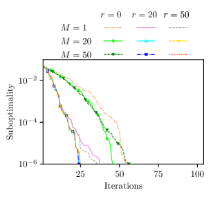
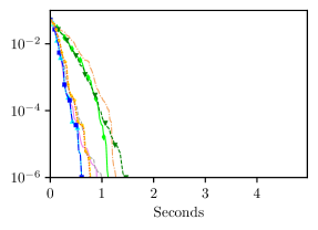
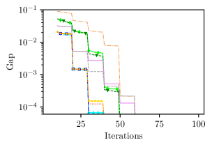
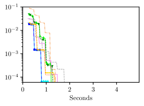
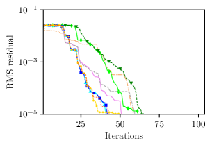
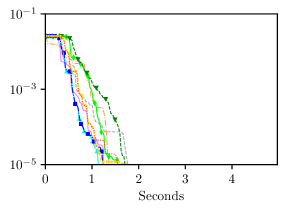
Figure 1: Suboptimality (top row), gap (middle row), and RMS residual (bottom row), versus iterations (left column) and run-time in seconds (right column) for OSMM on the Kelly gambling problem for the nine combinations of rank $r$ and memory $M$.

The timing results averaged from $10$ repetitions are shown in Table 1. The total solve time and iterations are based on achieving a high accuracy of $10^{-6}$, which is far more accurate than would be needed in practice. For our nine choices of algorithm parameters, the total OSMM time ranges from around 0.87 to 1.4 seconds, substantially faster than using MOSEK to solve the problem.

From the results in the figure and the table, as $r$ increases the convergence becomes faster in terms of iterations, but with a larger $r$ the update of $x^{k+1/2}$ takes more time, so each iteration becomes more expensive. A good trade-off value is $r=20$. The memory $M$ taking values $20$ and $50$ yields faster convergence in iterations and smaller gaps than $M$ taking value $0$, but as $M$ increases each iteration also becomes more expensive, and the run-time efficiency is the best when $M=20$. In summary, we see that rank value $r=20$ and memory value $M=20$ yield the fastest convergence in terms of run-time. We have observed this in other problem instances as well, so these are the default values in OSMM.

Table 1: Times to evaluate tentative update $x^{k+1/2}$ and lower bound $L_{k}$, total solve time and iterations to reach $10^{-6}$ accuracy, and average number of evaluations of $f$ per iteration, for OSMM with the nine combinations of rank $r$ and memory $M$.

Rank and memory		Compute times (sec.)		Total solve time and iterations
$r$	$M$	$x^{k+1/2}$	$L_{k}$	Time (sec.)	Iterations	$f$ evals./iter.
0	1	0.016	0.0069	1.4	62	4.1
0	20	0.019	0.0093	1.2	49	3.5
0	50	0.023	0.015	1.3	49	3.4
20	1	0.019	0.0069	0.88	36	2.9
20	20	0.023	0.0093	0.87	33	2.9
20	50	0.029	0.014	0.90	33	2.9
50	1	0.021	0.0076	0.92	32	2.5
50	20	0.027	0.010	0.88	29	2.5
50	50	0.035	0.015	0.89	29	2.5

4 Generic applications

In this section we describe some generic applications that reduce to our specific oracle-structured composite function minimization problem. We focus on the function $f$, which should be differentiable, but not so simple that it can be handled directly in a structured optimization system. We will see that this generally occurs when there is a lot of data required to specify $f$.

4.1 Stochastic programming

Sample average approximation for stochastic programming.

We start with the problem of minimizing $\mathop{\bf E{}}F(x,\omega)+g(x)$, where $F$ is convex in $x$ for each value of the random variable $\omega$. We will approximate the first objective term using a sample average. We generate $N$ independent samples $\omega_{1},\ldots,\omega_{N}$, and take

$$f(x)=\frac{1}{N}\sum_{i=1}^{N}F(x,\omega_{i}).$$ (31)

As a variation we can use importance sampling to get a lower variance estimate of $\mathop{\bf E{}}F(x,\omega)$. To do this we generate the samples from a proposal distribution with density $q$, and form the sample average estimate

$$f(x)=\frac{1}{N}\sum_{i=1}^{N}\frac{p(\omega_{i})}{q(\omega_{i})}F(x,\omega_{i}),$$ (32)

where $p$ is the density of $\omega$.

In both cases we can take $N$ to be quite large, since we will only need to evaluate $f$ and its gradient, and current systems for this are very efficient. For example, the gradients $\nabla F(x,\omega_{i})$ can be computed in parallel. As a practical matter, this happens automatically, with no or very little directive from the user who specifies $f$.

Validation and stopping criterion tolerance.

The functions $f$ given in (31) and (32) are only approximations of the true objective $\mathop{\bf E{}}F(x,\omega)$, though we hope they are good approximations when we take $N$ large, as we can with OSMM. To understand how accurate the sample average (31) is, we generate another set of independent samples $\tilde{\omega}_{1},\ldots,\tilde{\omega}_{N}$ and define the validation function as

$$f^{\mathrm{val}}(x)=\frac{1}{N}\sum_{i=1}^{N}F(x,\tilde{\omega}_{i})$$

(and similarly if we use importance sampling). The magnitude of the difference $|f^{\mathrm{val}}(x)-f(x)|$ gives us a rough idea of the accuracy in approximating $\mathop{\bf E{}}F(x,\omega)$. (Better estimates of the accuracy can be obtained by repeating this multiple times, but we are interested in only a crude estimate.)

Solving the oracle-structured problem to an accuracy substantially better than the Monte Carlo sampling accuracy does not make sense in practice. This justifies replacing the absolute gap tolerance $\epsilon_{\mathrm{abs}}^{\mathrm{gap}}$ with the maximum of a fixed absolute tolerance and the sampling error $|f^{\mathrm{val}}(x^{k})-f(x^{k})|$. (We can evaluate the sampling error whenever we evaluate the gap, i.e., every 10 iterations.) Roughly speaking, we stop when we know we have solved the problem to an accuracy that is better than our approximation.

4.2 Utility maximization

An important special case of stochastic optimization is utility maximization, where we seek to maximize

$$\mathop{\bf E{}}U(H(x,\omega))-g(x),$$ (33)

where $U:{\mbox{\bf R}}\to{\mbox{\bf R}}$ is a concave increasing utility function, and $H$ is concave in $x$ for each $\omega$. The first term, the expected utility, is concave. This is equivalent to the stochastic programming problem of minimizing

$$\mathop{\bf E{}}(-U(H(x,\omega))+g(x),$$

which is stochastic programming with $F=-U\circ H$, which is convex in $x$. We can replace the expectation with a sample average using (31), or an importance sampling sample average using (32). Utility maximization is a common method for handling the variance or uncertainty in a stochastic objective; it introduces risk aversion.

4.3 Conditional and entropic value-at-risk programming

Another method to introduce risk aversion into a stochastic optimization problem is to mimimize value-at-risk (VaR), or a specific quantile of $F(x,\omega)$, where $F$ is convex in $x$ for each value of the random variable $\omega$. The value-at-risk is defined as

$$\mathop{\bf VaR}(F(x,\omega);\eta)=\inf\{\gamma\mid\mathop{\bf Prob}(F(x,\omega)\leq\gamma)\geq\eta\},$$

where $\eta\in(0,1)$ is a given quantile. With an additional structured convex function $g$ in the objective, we obtain the VaR problem

$$\begin{array}[]{ll}\mbox{minimize}&\mathop{\bf VaR}(F(x,\omega);\eta))+g(x),\end{array}$$ (35)

which, roughly speaking, is the problem of minimizing the $\eta$-quantile of the random variable $F(x,\omega)+g(x)$. Aside from a few special cases, this problem is not convex. (Recent work on VaR and methods for the closely related problem of handling probability constraints can be found in, e.g., danielsson2013fat ; danielsson2008optimal .) We proceed by replacing the nonconvex VaR term with a convex upper bound on VaR, such as conditional value-at-risk (CVaR) CVAR_uryasev_rockafellar ; rockafellar2002conditional or entropic value-at-risk (EVaR) ahmadi2011information . Beyond resulting in tractable convex problems, these upper bounds possess a number of nice properties, such as being coherent risk measures; see rockafellar2002conditional ; ahmadi2011information for a discussion.

CVaR is given by

$$\mathop{\bf CVaR}(F(x,\omega);\eta)=\inf_{\alpha\in\mathbf{R}}\Bigg{\{}\frac{\mathop{\bf E{}}(F(x,\omega)-\alpha)_{+}}{1-\eta}+\alpha\Bigg{\}},$$ (36)

where $(z)_{+}=\max\{z,0\}$, and EVaR is given by

$$\mathop{\bf EVaR}(F(x,\omega);\eta)=\inf_{\alpha>0}\Bigg{\{}\alpha\log\Bigg{(}\frac{\mathop{\bf E{}}\exp(F(x,\omega)/\alpha)}{1-\eta}\Bigg{)}\Bigg{\}}.$$ (37)

Both of these are convex functions of $x$. We have, for any $x$,

$$\mathop{\bf VaR}(F(x,\omega);\eta)\leq\mathop{\bf CVaR}(F(x,\omega);\eta)\leq\mathop{\bf EVaR}(F(x,\omega);\eta)$$

(see, e.g., ahmadi2011information ). With CVaR, we obtain the convex problem

$$\begin{array}[]{ll}\mbox{minimize}&\mathop{\bf CVaR}(F(x,\omega);\eta))+g(x),\end{array}$$

and similarly for EVaR.

We now show how the CVaR and EVaR problems can be approximated as oracle-structured problems. We start with CVaR. We generate independent samples $\omega_{i}$, $i=1,\ldots,N$, and replace the expectation with the empirical mean,

$$f(x,\alpha)=\frac{1}{N}\sum_{i=1}^{N}\frac{(F(x,\omega_{i})-\alpha)_{+}}{1-\eta}+\alpha,$$

with variables $x$ and $\alpha$. This function is jointly convex in $x$ and $\alpha$; minimizing over $\alpha$ gives $\mathop{\bf CVaR}(F(x,\omega);\eta)$ for the empirical distribution. We adjoin $\alpha$ to $x$ to obtain a problem in oracle-structured form, i.e., minimizing $f(x,\alpha)+g(x)$, over $x$ and $\alpha$. (That is, we take $(x,\alpha)$ as what we call $x$ in our general form.) While $f$ is not differentiable in $(x,\alpha)$, we have observed that our method still works very well.

For EVaR, we obtain

$$f(x,\alpha)=\alpha\log\Bigg{(}\frac{1}{N}\sum_{i=1}^{N}\frac{\exp(F(x,\omega_{i})/\alpha)}{1-\eta}\Bigg{)},$$

which is jointly convex in $x$ and $\alpha$. (To see convexity, we observe that $f$ is the perspective function of the log-sum-exp function; see (BoydVand04, , §3.2.6).) As with CVaR, minimizing over $\alpha$ yields $\mathop{\bf EVaR}(F(x,\omega);\eta)$ for the empirical distribution. Unlike our approximation with CVaR, this function is differentiable.

4.4 Generic exponential family density fitting

We consider fitting an exponential family of densities, given by

$$p_{\theta}(z)=e^{-\left(\phi(z)^{T}\theta+A(\theta)\right)},$$ (38)

to samples $z_{1},\ldots,z_{m}\in\mathcal{S}$. Here, $\mathcal{S}$ is the support of the density, $\phi:\mathcal{S}\to{\mbox{\bf R}}^{n}$ is the sufficient statistic, and $\theta\in\Theta\subseteq{\mbox{\bf R}}^{n}$ is the canonical parameter (to be fitted). The density normalizes via the log-partition (or cumulant generating) function

$$A(\theta)=\log\int_{\mathcal{S}}e^{-\phi(z)^{T}\theta}\;dz.$$

We assume $\Theta$ is convex, and additionally that it only contains parameters for which the log-partition function is finite.

The negative log-likelihood, given samples $z_{1},\ldots,z_{m}$, is

$$\sum_{i=1}^{m}\log p_{\theta}(z_{i})=c^{T}\theta+mA(\theta),$$

where $c=\sum_{i=1}^{m}\phi(z_{i})$. So maximum likelihood estimation of $\theta$ corresponds to solving the density fitting problem

$$\begin{array}[]{ll}\mbox{minimize}&\frac{1}{m}c^{T}\theta+A(\theta)+\lambda r(\theta)\\ \mbox{subject to}&\theta\in\Theta,\end{array}$$ (41)

with variable $\theta$. We can include a (potentially nonsmooth) convex regularization term $\lambda r(\theta)$ in the objective, where $\lambda\geq 0$ is the regularization strength, and $r:\Theta\to{\mbox{\bf R}}$ is the regularizer. Since the log-partition function is convex wainwright2008graphical , the density fitting problem (41) is also convex.

The log-partition function is generally intractable except for a few special cases, so we replace the integral in $A(\theta)$ with a finite sum using importance sampling, i.e.,

$$\int_{\mathcal{S}}e^{-\phi(z)^{T}\theta}\;dz\approx\frac{1}{N}\sum_{i=1}^{N}\frac{1(\omega_{i}\in\mathcal{S})}{q(\omega_{i})}e^{-\phi(\omega_{i})^{T}\theta},$$

where $\omega_{i},\;i=1,\ldots,N$, are independent draws from the proposal distribution $q$. The number of samples $N$ can be very large, especially when the number of dimensions $n$ is moderate. When $\mathcal{S}$ is bounded and its dimension is small, we can simply use a Riemann sum, so that the samples $\omega_{i}$ are lattice points in $\mathcal{S}$ and we have $q(\omega_{i})=1/|\mathcal{S}|$. The problem (41) is clearly in oracle-structured form, once we take $A(\theta)$ (with its Monte Carlo approximation) to be $f$, and the rest of the objective plus the indicator of $\Theta$ to be $g$.

A number of interesting regularizers are possible. The squared $\ell_{2}$ norm, i.e., $r(\theta)=\|\theta\|_{2}^{2}$, is of course a natural choice. When $\mathcal{S}$ is bounded, a different option is to use the squared $L_{2}$ norm of the gradient of the log-density

$$r(\theta)=\int_{\mathcal{S}}\|\nabla\log p_{\theta}(z)\|_{2}^{2}\;dz.$$

This regularizer enforces a certain kind of smoothness: the regularized density $p_{\theta}$ tends to the uniform distribution on $\mathcal{S}$, as the regularization strength $\lambda$ grows. Finally, observe that we can write

$$\int_{\mathcal{S}}\|\nabla\log p_{\theta}(z)\|_{2}^{2}\;dz=\int_{\mathcal{S}}\|D\phi(z)^{T}\theta\|_{2}^{2}\;dz=\theta^{T}\left(\int_{\mathcal{S}}D\phi(z)D\phi(z)^{T}\;dz\right)\theta,$$

where $D\phi$ is the Jacobian of sufficient statistic $\phi$. We can replace the integral with a finite sum again, and obtain the regularizer

$$r(\theta)\approx\theta^{T}\left(\frac{1}{N}\sum_{i=1}^{N}\frac{1(\omega_{i}\in\mathcal{S})}{q(\omega_{i})}D\phi(\omega_{i})D\phi(\omega_{i})^{T}\right)\theta.$$

5 Numerical examples

In this section we demonstrate the performance of OSMM through several numerical examples, all taken from the generic applications described in the previous section. We start by showing results for two different portfolio selection problems, the Kelly gambling example (shown earlier in §3.2), and minimizing CVaR. We then show a density estimation example. After that we present results for a supply chain optimization problem with entropic value-at-risk minimization. All of these examples are structured stochastic optimization problems, and we use simple sample averages to approximate expectations. OSMM is designed to handle the case when $f$ is complex, which in the case of sample averages means $N$ is large. We will see that when $N$ is small, OSMM is actually slower than just solving the problem directly using a structured solver; when $N$ is large, it is much faster (and in many cases, directly using a structured solver fails).

We report the time needed for OSMM to reach high accuracy, i.e., $h(x^{k})-h^{\star}\leq 10^{-6}$. (This makes a fairer comparison with MOSEK, SCS ocpb:16 ; scs , and ECOS.) We also indicate when practical accuracy is reached, using our default parameters, and the sampling accuracy. We use the default parameters in OSMM, and use ECOS as the solver in CVXPY to compute the tentative iterate $x^{k+1/2}$. We do not perform any parameter tuning for our method.

5.1 Kelly gambling

Problem formulation.

In the Kelly gambling problem there are $n$ bets we can wager on, and $N$ possible outcomes, with probabilities $\pi_{i}$, $i=1,\ldots,N$. The bet returns are given by $r_{i}\in{\mbox{\bf R}}_{+}^{n}$, where $(r_{i})_{j}$ is the return, i.e., the amount you win for each dollar you put on bet $j$ when outcome $i$ occurs. We are to choose $x\in{\mbox{\bf R}}^{n}$, with $\mathbf{1}^{T}x=1$, where $x_{j}$ is the fraction of our wealth we place on bet $j$. We seek to maximize the average log return, which maximizes long-term wealth growth if we repeatedly bet. This leads to the (convex) optimization problem

$$\begin{array}[]{ll}\mbox{maximize}&\sum_{i=1}^{N}\pi_{i}\log(r_{i}^{T}x)\\ \mbox{subject to}&x\geq 0,\quad\mathbf{1}^{T}x=1,\end{array}$$

with variable $x$.

Problem instance.

We consider $n=200$ bets. The probabilities of the outcomes $\pi_{i}$ are independent draws from a uniform distribution on $[0,1]$, normalized to sum to one. The returns of the bets in each outcome are independently drawn from a log normal distribution, i.e., $\exp(z)$, $z\sim\mathcal{N}(0,1)$, and then scaled so the expected return of bet $j$ is $\bar{r}_{j}$, i.e., $\sum_{i=1}^{N}\pi_{i}(r_{i})_{j}=\bar{r}_{j}$, where $\bar{r}_{j}$ is drawn from a uniform distribution on $[0.9,1.1]$. For our problem instance, the solution has 57 nonzero entries ranging from 0.001 to 0.04, and the optimal mean log return is 0.057.

Results.

The run-times for OSMM, MOSEK, SCS, and ECOS are shown in table 2. When the number of Monte Carlo samples is small, e.g., $N=1{,}000$, MOSEK performs the fastest and takes less than a second to attain high accuracy. OSMM also takes less than one second. ECOS takes about two seconds, and SCS takes roughly six seconds. However, when $N$ is larger (i.e., $N=10{,}000$, $100{,}000$, or $1{,}000{,}000$), OSMM is the fastest method, always taking less than a second to attain the required $10^{-6}$ optimality gap. When $N=10{,}000$, MOSEK is still competitive, but SCS and ECOS are two to four orders of magnitude slower than OSMM. When $N=100{,}000$, MOSEK and ECOS are two to three orders of magnitude slower, and when $N=1{,}000{,}000$, MOSEK and ECOS are three to five orders of magnitude slower. SCS fails for both the two larger values of $N$. These findings suggest that OSMM is useful when the number of samples is large, as it exhibits good scaling with $N$.

OSMM spends 0.0013 and 0.0024 seconds to evaluate $f$ and its gradient $\nabla f$, respectively, when $N=1{,}000{,}000$. Computing the tentative iterate $x^{k+1/2}$ and the lower bound $L_{k}$ from (5) takes 0.033 and 0.014 seconds, respectively. The line search also turns out to be quite efficient here, as $f$ is evaluated twice during the line search on average.

Table 2: Solve times in seconds on the Kelly gambling problem. A dash (“—”) means the solver failed, either for numerical reasons, or because it did not reach the required $10^{-6}$ suboptimality in 24 hours.

$N$	OSMM	MOSEK	SCS	ECOS
1,000	0.76	0.58	6.4	2.2
10,000	0.64	4.5	2,100	50
100,000	0.62	62	—	910
1,000,000	0.64	890	—	20,000

Figure 2 shows the convergence of OSMM with $N=1{,}000{,}000$. In the top panel, we can see that practical accuracy is reached after 14 iterations, and high accuracy is reached after 16 iterations, as shown by the dotted black and green lines, respectively.

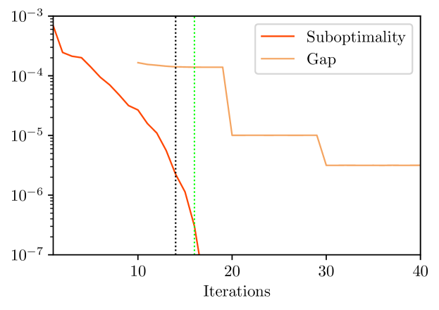
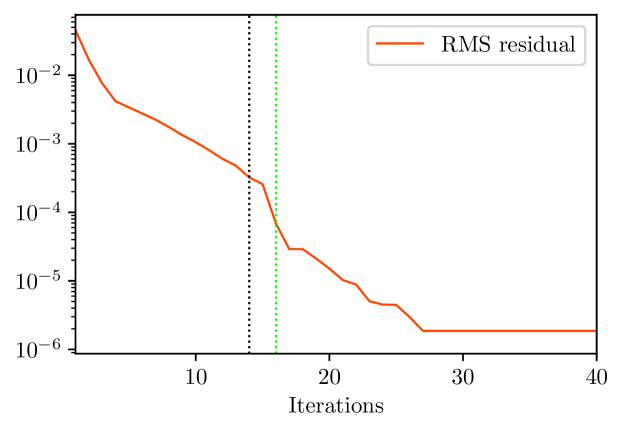
Figure 2: Suboptimality, gap (top row), and RMS residual (bottom row) on the Kelly gambling problem with $N=1{,}000{,}000$. The dotted green and black lines show when high accuracy and practical accuracy are reached, respectively.

5.2 CVaR portfolio optimization with derivatives

Problem formulation.

We consider making investments in $m$ stocks, and call and put derivatives on them, with various strike prices. Our investment will be for one period (of, say, one month). We let $\omega\in{\mbox{\bf R}}_{++}^{m}$ denote the (fractional) change in prices of the $m$ underlying stocks, which we model as random with a log-normal distribution, i.e., $\log\omega\sim\mathcal{N}(\mu,\Sigma)$, where the $\log$ is elementwise. For simplicity we will assume there is one call and one put option available for each stock. Let $p_{\text{c}}\in{\mbox{\bf R}}_{++}^{m}$ and $s_{\text{c}}\in{\mbox{\bf R}}_{++}^{m}$ be the call option prices (premia) and strike prices, normalized by the current stock price, so, for example, $(s_{\text{c}})_{i}=1.15$ means the strike price is $1.15$ times the current stock price. Let $p_{\text{p}}\in{\mbox{\bf R}}^{m}_{++}$ and $s_{\text{p}}\in{\mbox{\bf R}}^{m}_{++}$ denote the corresponding quantities for the $m$ put options.

The amount we receive per dollar of investment in the underlying stocks is $\omega$, the ratio of the current to final stock price. For every dollar invested in the call options we receive $(\omega-s_{\text{c}})_{+}/p_{\text{c}}$, where the division is elementwise, and $(a)_{+}=\max\{a,0\}$. For the put options, the total we receive per dollar of investment is $(s_{\text{p}}-\omega)_{+}/p_{\text{p}}$.

We make investments in $n=3m$ different assets, the $m$ underlying stocks and $m$ associated call and put options. We let $x\in{\mbox{\bf R}}^{n}$ denote the fractions of our wealth that we invest in the assets, so $\mathbf{1}^{T}x=1$. We consider long and short positions, with $x_{i}<0$ denoting a short position. We consider a simple set of portfolio constraints, $x\geq x_{\text{min}}$ (e.g., $x_{\text{min}}=-0.1$ limits the maximum short position for any asset to not exceed 10% of the total portfolio value), and $\|x\|_{1}\leq L$, where $L$ is a leverage limit. (Since $\mathbf{1}^{T}x=1$, this means that the total long position cannot exceed a multiple $(L+1)/2$ of total wealth, and the total short position cannot exceed a multiple $(L-1)/2$ of the total wealth.) We partition $x$ as $x=(x_{\text{u}},x_{\text{c}},x_{\text{p}})$, with each subvector in ${\mbox{\bf R}}^{m}$. Our portfolio has total return

$$x_{\text{u}}^{T}\omega+x_{\text{c}}^{T}((s_{\text{c}}-\omega)_{+}/p_{\text{c}})+x_{\text{p}}^{T}((s_{\text{p}}-\omega)_{+}/p_{\text{p}})=r(\omega)^{T}x,$$

where $r(\omega)\in{\mbox{\bf R}}^{n}$ is the total return of the $n=3m$ assets, i.e., stocks and options.

Our problem is to choose the portfolio so as to minimize the conditional value at risk (described in (36)) of the negative total return, i.e.,

$$\begin{array}[]{ll}\mbox{minimize}&\mathop{\bf CVaR}(-r(\omega)^{T}x;\eta)\\ \mbox{subject to}&x\geq x_{\text{min}},\;\mathbf{1}^{T}x=1,\;\|x\|_{1}\leq L,\end{array}$$

where $\eta\in(0,1)$ sets the risk aversion.

We use a sample average approximation of the expectation in CVaR to obtain the problem

$$\begin{array}[]{ll}\mbox{minimize}&\frac{1}{N}\sum_{i=1}^{N}\frac{(-r(\omega_{i})^{T}x-\alpha)_{+}}{1-\eta}+\alpha\\ \mbox{subject to}&x\geq x_{\text{min}},\;\mathbf{1}^{T}x=1,\;\|x\|_{1}\leq L\end{array}$$

with variables $x=(x_{\text{u}},x_{\text{c}},x_{\text{p}})\in{\mbox{\bf R}}^{n}$ and $\alpha\in{\mbox{\bf R}}$. The vectors $\omega_{i}\in{\mbox{\bf R}}_{++}^{n}$, $i=1,\ldots,N$, are independent samples of the price change $\omega$.

Problem instance.

We take the number of stocks as $m=100$, so $n=300$. We take the minimum position limit $x_{\text{min}}=-0.1$ and leverage limit $L=1.6$. We use risk aversion parameter $\eta=0.8$, so we are attempting to minimize the 20th percentile of the portfolio loss. The price change covariance $\Sigma$ is generated according to $\Sigma=\sigma^{2}(I+0.2FF^{T})$, where $\sigma=1/\sqrt{2}$, and the entries of $F\in{\mbox{\bf R}}^{m\times 5}$ are independent draws from a standard normal distribution. We set the mean price change according to $\mu_{i}=0.03\sqrt{\Sigma_{ii}}-0.5\Sigma_{ii}$, $i=1,\ldots,m$. For each call option, the strike price is set as the 80th percentile of $\omega$, and for each put option it is the 20th percentile. The option prices are determined by the Black-Scholes formula with zero discount. (These data are approximately consistent with an investment period of one month for U.S. equities.)

When we solve this problem instance, the optimal portfolio return has mean 1.3%, standard deviation 5%, and loss probability 39%; annualized, these correspond to a return of 16%, standard deviation 18%, and loss probability 20%. The optimal portfolio contains as assets the underlying stocks as well as call and put options.

Results.

Table 3 shows the run-times for $N$ ranging from $10{,}000$ to $1{,}000{,}000$. We see again that for small values of $N$, it is more efficient to solve the problem directly using a structured solver, whereas for large values, OSMM is far more efficient. When $N=1{,}000{,}000$, OSMM (using PyTorch) takes 0.0021 seconds to evaluate $f$ and 0.0053 seconds to evaluate $\nabla f$; OSMM takes 0.050 seconds to compute the tentative iterate $x^{k+1/2}$, and 0.021 seconds to evaluate the lower bound $L_{k}$ (using CVXPY). Figure 3 shows the convergence of OSMM with $N=1{,}000{,}000$. Practical accuracy are high accuracy are reached at the same time after 100 iterations.

Table 3: Solve times in seconds on the conditional value-at-risk problem. A dash (“—”) means the solver failed, either for numerical reasons, or because it did not reach the required $10^{-6}$ suboptimality in 24 hours.

$N$	OSMM	MOSEK	SCS	ECOS
10,000	11	6.0	250	18
100,000	6.5	64	2,900	310
1,000,000	6.3	1,900	30,000	5,200

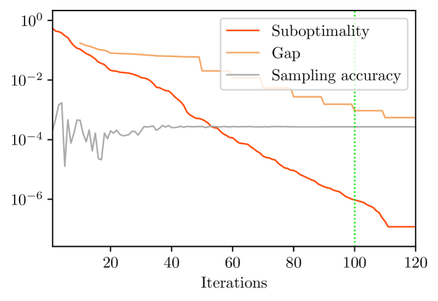
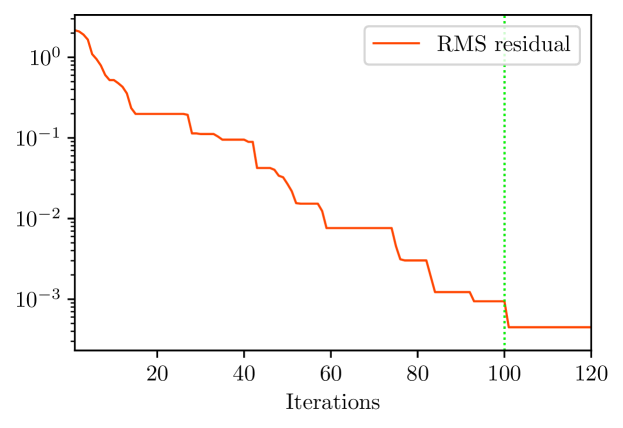
Figure 3: Suboptimality, gap, sampling accuracy (top row), and RMS residual (bottom row) on the conditional value-at-risk problem with $N=1{,}000{,}000$. The dotted green and black lines coincide, indicating that high accuracy and practical accuracy are reached at the same time.

5.3 Exponential series density estimation

Problem formulation.

We consider an instance of the generic exponential family density fitting problem described in §4.4. We consider data $z_{1},\ldots,z_{m}\in{\mbox{\bf R}}^{2}$, and wish to fit a density $p$ supported on $\mathcal{S}=[-1,1]^{2}$. We let the sufficient statistics $\phi_{i},\;i=1,\ldots,n$, be the Legendre polynomials up to degree four, so $n=14$. (This is known as an exponential series density estimator marsh2007goodness ; wu2010exponential ; gao2015penalized .) We solve the density estimation problem (41).

Problem instance.

We take $m$ data points sampled from a mixture of three Gaussian densities, restricted to $\mathcal{S}$, with means $(1/3,1/3)$, $(1/3,-1/3)$, and $(-1/3,-1/3)$, weights $0.4$, $0.3$, and $0.3$, and common covariance $(1/36)I$. (So the data do not come from the family of density we use to fit.) We form a Riemann sum using points in $\mathcal{S}$ lying on a grid with side lengths $\sqrt{N}$. Recall that $N$, the number of samples, here refers to our approximate evaluation of the integral that arises in the log-partition function, and not the number of data samples, which is fixed at $m=2{,}000$.

Results.

Table 4 shows the run-times for the various methods. We see the usual pattern where directly solving the problem can be efficient for small $N$, but OSMM is much faster for large $N$. When $N=1{,}000{,}000$, it takes OSMM 0.001 and 0.0014 seconds to evaluate $f$ and $\nabla f$, respectively, and 0.015 and 0.0097 seconds to compute $x^{k+1/2}$ and $L_{k}$, respectively.

Figure 4 shows the convergence of OSMM for $N=1{,}000{,}000$. Practical accuracy is reached after 39 iterations with suboptimality $10^{-5}$, and after 42 iterations OSMM reaches high accuracy. In this instance, our lower bound $L_{k}=-\infty$, so neither it nor the gap are plotted in the figure.

Table 4: Solve times in seconds on the density estimation problem. A dash (“—”) means the solver failed, either for numerical reasons, or because it did not reach the required $10^{-6}$ suboptimality in 24 hours.

$N$	OSMM	MOSEK	SCS	ECOS
10,000	0.72	1.2	1,100	0.92
100,000	1.2	11	—	14
1,000,000	0.84	120	—	190

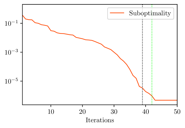
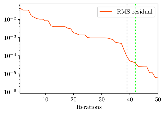
Figure 4: Suboptimality (top row) and RMS residual (bottom row) on the exponential family density fitting problem with $N=1{,}000{,}000$. The dotted green and black lines show when high accuracy and practical accuracy are reached, respectively.

5.4 Vector news vendor with entropic value-at-risk

We consider a variant of the classic news vendor problem that involves entropic value-at-risk programming ahmed2007coherent .

Problem formulation.

We choose quantities $q\in{\mbox{\bf R}}_{+}^{n}$ of $n$ products to produce, at total cost $\phi(q)$, where $\phi:{\mbox{\bf R}}^{n}_{+}\to{\mbox{\bf R}}_{+}$. We have constraints on the quantities we can produce, $q\leq q_{\mathrm{max}}$, and on the total production cost, $\phi(q)\leq\phi_{\mathrm{max}}$. We sell the amount $\min(q,d)$, where $d\in{\mbox{\bf R}}_{+}^{n}$ is the demand, and the min is taken elementwise, at market prices $p\in{\mbox{\bf R}}_{+}^{n}$, so the total revenue is $p^{T}\min(q,d)$, and the profit is

$$P=p^{T}\min\{q,d\}-\phi(q).$$

We assume that $\omega=(d,p)\in{\mbox{\bf R}}_{+}^{2n}$ is a random variable with known distribution, so $P(q,\omega)$ is a random variable that depends on $q$.

We choose the quantities $q$ to minimize the EVaR of the negative profit,

$$\begin{array}[]{ll}\mbox{minimize}&\mathop{\bf EVaR}(-P(q,\omega);\eta)\\ \mbox{subject to}&\phi(q)\leq\phi_{\max},\;q\geq 0,\;q\leq q_{\max},\end{array}$$

where $\eta$ is a specified quantile.

As described in §4.3, we approximate this with Monte Carlo samples $(d_{1},p_{1}),\ldots,(d_{N},p_{N})$ to obtain the problem

$$\begin{array}[]{ll}\mbox{minimize}&\alpha\log\left(\frac{1}{(1-\eta)N}\sum_{i=1}^{N}\exp\left(\frac{-p_{i}^{T}\min(q,d_{i})+\phi(q)}{\alpha}\right)\right)\\ \mbox{subject to}&\phi(q)\leq\phi_{\max},\;q\geq 0,\;q\leq q_{\max},\;\alpha\geq 0,\end{array}$$

with variables $q$ and $\alpha\in{\mbox{\bf R}}_{+}$. We denote the realizations of the demand $d$ and prices $p$ on the $i$th Monte Carlo simulation by $d_{i},p_{i}\in{\mbox{\bf R}}_{+}^{n},\;i=1,\ldots,N$, respectively.

Problem instance.

We take $n=500$ and risk aversion parameter $\eta=0.9$. We assume the demand and market prices follow a joint log-normal distribution, i.e., $(d,p)=\exp z$, $z\sim\mathcal{N}(\mu,\Sigma)$, and the exponential is elementwise. We draw the entries of $\mu\in{\mbox{\bf R}}^{2n}$ independently from a uniform distribution on $[-0.2,0]$, and set $\Sigma=0.1FF^{T}$, where the entries of $F\in{\mbox{\bf R}}^{2n\times 5}$ are independently drawn from a standard normal distribution. We use a production cost which is separable and piecewise affine with one kink point for each entry of $q$,

$$\phi(q)=a^{T}q+0.5a^{T}(q-b)_{+},$$

where the elements in $a$ and $b$ are both drawn uniformly at random from $[0.2,0.9]$ and $[0.01,0.03]$, respectively. The maximum production quantities $q_{\max}$ is set as $5b$, and the maximum cost is $\phi_{\textrm{max}}=1$. With these parameter values, the optimal profit has mean 3.2 and standard deviation 0.98.

Results.

The run-times for the various methods are in table 5. In this instance, OSMM is the fastest for all values of $N$ ranging from $1{,}000$ to $1{,}000{,}000$, and the other solvers fail for nearly all values of $N$. When $N=1{,}000{,}000$, OSMM takes 0.16 and 0.27 seconds to evaluate $f$ and $\nabla f$, respectively; it takes 0.076 seconds to compute the tentative iterate, and 0.036 seconds to compute the lower bound.

Figure 5 shows the convergence of OSMM with $N=1{,}000{,}000$. We can see that practical accuracy is reached after 50 iterations with suboptimality on the order of $10^{-5}$, while it takes 58 iterations to reach high accuracy.

Table 5: Solve times in seconds on the vector news vendor problem. A dash (“—”) means the solver failed, either for numerical reasons, or because it did not reach the required $10^{-6}$ suboptimality in 24 hours.

$N$	OSMM	MOSEK	SCS	ECOS
1,000	6.7	120	—	—
10,000	11	7,400	—	—
100,000	10	—	—	—
1,000,000	53	—	—	—

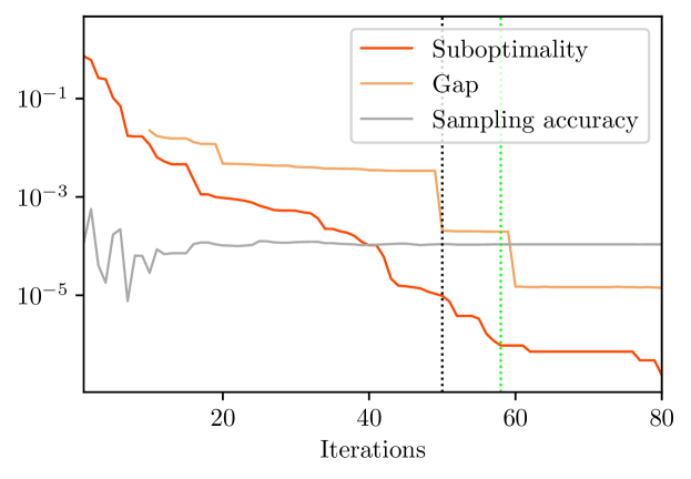
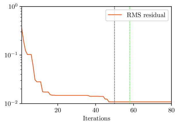
Figure 5: Suboptimality, gap, sampling accuracy (top row), and RMS residual (bottom row) on the vector news vendor problem with $N=1{,}000{,}000$. The dotted green and black lines show when high accuracy and practical accuracy are reached, respectively.

Appendix A Appendix

A.1 Details of forming $G_{k}$

We form $G_{k}$ in (3) by adopting a quasi-Newton update given in fletcher2005new . The main idea is to divide $G_{k}$ into two matrices $G_{k}^{(1)}$ and $G_{k}^{(2)}$, which are the first $r_{1}$ and the last $r_{2}=r-r_{1}$ columns in $G_{k}$, respectively, and update them separately into $G_{k+1}^{(1)}$ and $G_{k+1}^{(2)}$. Then $G_{k+1}$ is updated by

$$G_{k+1}=\left[G^{(1)}_{k+1}\quad G^{(2)}_{k+1}\right].$$

The detail is as follows. Let $s_{k}=x^{k+1}-x^{k}$ and $y_{k}=\nabla f(x^{k+1})-\nabla f(x^{k})$. From the convexity of $f$, $s_{k}^{T}y_{k}\geq 0$. Suppose that $s_{k}^{T}y_{k}$ is not too small such that

$$s_{k}^{T}y_{k}>\max(\varepsilon_{\mathrm{abs}},\varepsilon_{\mathrm{rel}}\|s_{k}\|_{2}\|y_{k}\|_{2}),$$ (42)

where constants $\varepsilon_{\mathrm{abs}},\varepsilon_{\mathrm{rel}}>0$ are given. Then $r_{1}$ is chosen as the largest integer in $[0,r]$ such that $G_{k}^{(1)}$ satisfies

$$s_{k}^{T}y_{k}-\left\|(G_{k}^{(1)})^{T}s_{k}\right\|_{2}^{2}>\varepsilon_{\mathrm{rel}}\|s_{k}\|_{2}\left\|y_{k}-G_{k}^{(1)}(G_{k}^{(1)})^{T}s_{k}\right\|_{2}.$$

According to (42) the above holds at least for $r_{1}=0$, in which case $G^{(1)}_{k}$ degenerates to $0$.

Once $r_{1}$ is obtained, we define $w_{k}^{(1)}=(G^{(1)}_{k})^{T}s_{k}$ and $w_{k}^{(2)}=(G^{(2)}_{k})^{T}s_{k}$. Then $R_{k}^{(1)}\in{\mbox{\bf R}}^{(r_{1}+1)\times(r_{1}+1)}$ is the upper triangular factor in the following R-Q decomposition

$$R_{k}^{(1)}Q_{k}^{(1)}=\left[\begin{array}[]{ll}\frac{1}{\sqrt{s_{k}^{T}y_{k}-\|w_{k}^{(1)}\|_{2}^{2}}}&0_{r_{1}}^{T}\\ \frac{-1}{\sqrt{s_{k}^{T}y_{k}-\|w_{k}^{(1)}\|_{2}^{2}}}w_{k}^{(1)}&I_{r_{1}}\end{array}\right]\in{\mbox{\bf R}}^{(r_{1}+1)\times(r_{1}+1)},$$

and $Q_{k}^{(2)}\in{\mbox{\bf R}}^{r_{2}\times(r_{2}-1)}$ is a set of orthonormal basis orthogonal to $w_{k}^{(2)}$. The update is

$$G^{(1)}_{k+1}=\left[y_{k}\quad G^{(1)}_{k}\right]R_{k}^{(1)},\quad G^{(2)}_{k+1}=G^{(2)}_{k}Q_{k}^{(2)}.$$

There are some corner cases. If (42) holds and $r_{1}=0$, then $G_{k+1}^{(1)}=y_{k}/\sqrt{s_{k}^{T}y_{k}}$. If $r_{1}=r-1$ or $r_{1}=r$, then $G_{k+1}^{(2)}$ vanishes, and $G_{k+1}$ takes the first $r$ columns of $G_{k+1}^{(1)}$.

In cases where (42) does not hold, if $\|w_{k}^{(2)}\|_{2}>\varepsilon_{\mathrm{abs}}$, then we can still define $G_{k+1}^{(2)}$ in the same way, and $G_{k+1}=\left[G^{(2)}_{k+1}\quad 0_{n}\right].$ Otherwise, $G_{k+1}=G_{k}$.

It can be easily checked that by the $G_{k}$ defined as above, the trace of $H_{k}$ is uniformly upper bounded in $k$.

The default values for the parameters are $\varepsilon_{\mathrm{abs}}=10^{-8}$ and $\varepsilon_{\mathrm{rel}}=10^{-3}$.

A.2 Details of computing an optimal subgradient of $g$

Here we show how to compute a subgradient $q^{k+1}\in\partial g(x^{k+1/2})$ satisfying the optimality conditions in (8), which implies (10). This, in turn, is important because it allows us to compute the stopping criteria described in §2.6.

Since we know the third term on the right-hand side of (8), it suffices to find an optimal subgradient $l_{k}^{k+1/2}\in\partial l_{k}(x^{k+1/2})$, which is easier. We start by rewriting the defining problem for $x^{k+1/2}$ in a more useful form. Putting (4) and (7) together, we see that we can alternatively express $x^{k+1/2}$ as the solution to the convex problem

$$\begin{array}[]{ll}\mbox{minimize}&z+g(x)+\frac{1}{2}(x-x^{k})^{T}(H_{k}+\lambda_{k}I)(x-x^{k})\\ \mbox{subject to}&z\geq f(x^{i})+\nabla f(x^{i})^{T}(x-x^{i}),\quad\textrm{for }i=\max\{0,k-M+1\},\ldots,k,\end{array}$$ (43)

with variables $x$ and $z\in{\mbox{\bf R}}$.

The KKT conditions for problem (43), which are necessary and sufficient for the points $(x^{k+1/2},z^{k+1/2})$ and $\gamma_{i},\;i=\max\{0,k-M+1\},\ldots,k$, to be primal and dual optimal, are

$$z^{k+1/2}\geq f(x^{i})+\nabla f(x^{i})^{T}(x^{k+1/2}-x^{i}),\quad i=\max\{0,k-M+1\},\ldots,k;$$ (44)

$$\sum_{i=\max\{0,k-M+1\}}^{k}\gamma_{i}=1,\quad\gamma_{i}\geq 0,\quad i=\max\{0,k-M+1\},\ldots,k;$$ (45)

$$z^{k+1/2}>f(x^{i})+\nabla f(x^{i})^{T}(x^{k+1/2}-x^{i})\implies\gamma_{i}=0,\quad i\in\max\{0,k-M+1\},\ldots,k;$$ (46)

$$\partial g(x^{k+1/2})+(H_{k}+\lambda_{k}I)v^{k}+\sum_{i=\max\{0,k-M+1\}}^{k}\gamma_{i}\nabla f(x^{i})\ni 0.$$ (47)

Here we used the definition of $v^{k}$ to simplify the stationarity condition (47).

Now we claim that

$$l_{k}^{k+1/2}=\sum_{i=\max\{0,k-M+1\}}^{k}\gamma_{i}\nabla f(x^{i})\in\partial l_{k}(x^{k+1/2}).$$

To see this, note that (45) says the $\gamma_{i}$ are nonnegative and sum to one, while (44) and (46) together imply $\gamma_{i}$ is positive as long as $\nabla f(x^{i})$ is active; this satisfies (9), which says the subdifferential $\partial l_{k}(x^{k+1/2})$ is the convex hull of the active gradients. Therefore, re-arranging (47) gives

$$q^{k+1}=-l_{k}^{k+1/2}-(H_{k}+\lambda_{k}I)v^{k}\in\partial g(x^{k+1/2}),$$

which shows (10).

A.3 Proof that undamped steps occur infinitely often

Assume that $\nabla f$ is Lipschitz continuous with constant $L$. Also, assume $\mu_{\max}\tau_{\min}>2L/(1-\alpha)$. We show that for any number of iterations $k_{0}$, there is some $k\geq k_{0}$ such that $t_{k}=1$. This means that there exists a subsequence $(k_{\ell})_{\ell=1}^{\infty}$ such that $t_{k_{\ell}}=1$.

To show the result, we first claim that the line search condition (20) is satisfied as soon as

$$t_{k}\leq\frac{1-\alpha}{2L}\lambda_{k}.$$ (48)

We prove the claim later. Taking the claim as a given for now, the main result follows by deriving a contradiction. To get a contradiction, suppose there exists some number of iterations $k_{0}$ such that $t_{k}<1$ for each $k\geq k_{0}$. Then, because $t_{k}$ is the largest number satisfying $t_{k}=\beta^{j}$ ($j\in\mbox{\bf{N}}_{0}$) and the line search condition, we get that the line search condition does not hold with $t_{k}=1$, and thus (48) does not hold with $t_{k}=1$, meaning that $\lambda_{k}<2L/(1-\alpha)$, for each $k\geq k_{0}$. But from (23), we have $\mu_{k}=\min\left\{\gamma_{\mathrm{inc}}^{k-k_{0}}\mu_{k_{0}},\mu_{\max}\right\}$, since we assumed $t_{k}<1$ for every $k\geq k_{0}$. Additionally, from (22), we get $\lambda_{k}\geq\mu_{k}\tau_{\min}$. So, we now have two cases. Either we have $\lambda_{k}\geq\mu_{\max}\tau_{\min}>2L/(1-\alpha)$, which is a contradiction with $\lambda_{k}<2L/(1-\alpha)$. Or we have $\lambda_{k}\geq\gamma_{\mathrm{inc}}^{k-k_{0}}\mu_{k_{0}}\tau_{\min}$, in which case $\gamma_{\mathrm{inc}}^{k-k_{0}}\mu_{k_{0}}\tau_{\min}$ grows exponentially in $k$; this means we must have $\lambda_{k}\geq 2L/(1-\alpha)$, for $k$ sufficiently large, which is again a contradiction. This finishes the proof of the main result.

Now we prove the claim. Observe that

$$Lt_{k}^{2}\|v^{k}\|^{2}\leq\frac{1-\alpha}{2}\lambda_{k}t_{k}\|v^{k}\|^{2}\leq\frac{1-\alpha}{2}t_{k}(v^{k})^{T}(H_{k}+\lambda_{k}I)v^{k},$$ (49)

where we used (48) to get the first inequality. We now use the following two facts: $\nabla f$ being $L$-Lipschitz continuous implies that (i) $\phi_{k}$ is convex in $t$, and (ii) $\phi_{k}^{\prime}$ is $L\|v^{k}\|^{2}$-Lipschitz in $t$. By the first fact (convexity), we have

$$\phi_{k}(t_{k})\leq\phi_{k}(0)+\phi_{k}^{\prime}(t_{k})t_{k}.$$

Adding and subtracting $\phi_{k}^{\prime}(0)$ gives

$$\phi_{k}(t_{k})\leq\phi_{k}(0)+\phi_{k}^{\prime}(0)t_{k}+(\phi_{k}^{\prime}(t_{k})-\phi_{k}^{\prime}(0))t_{k}.$$

The second fact (Lipschitz continuity) yields a bound on the third term on the right-hand side,

$$\phi_{k}(t_{k})\leq\phi_{k}(0)+\phi_{k}^{\prime}(0)t_{k}+Lt_{k}^{2}\|v^{k}\|^{2}.$$ (50)

Finally, using (18) and (49) to bound $\phi_{k}^{\prime}(0)$ and $Lt_{k}^{2}\|v^{k}\|_{2}^{2}$ in (50) yields (20), which implies the line search condition (20) is satisfied, as claimed.

We note that the claim above also implies the following lower bound, which is used in §3.1. Observe that if $t_{k}$ indeed satisfies the line search condition, then we can express $t_{k}=\beta^{j}$, where $j$ is the smallest integer such that (48) holds (see §2.4). Now consider two cases. If $1\leq(1-\alpha)\lambda_{k}/(2L)$, then we can simply take $j=0$, so that $t_{k}=1$. On the other hand, if $1>(1-\alpha)\lambda_{k}/(2L)$, then a short calculation shows that $j=\lceil\log_{\beta}((1-\alpha)\lambda_{k}/(2L))\rceil$, and so $j<1+\log_{\beta}((1-\alpha)\lambda_{k}/(2L))$, giving $t_{k}=\beta^{j}>\beta(1-\alpha)\lambda_{k}/(2L)$. Therefore, to sum up, we have (48) implies that $t_{k}$ satisfies the inequalities

$$t_{k}>\beta\min\left\{1,\frac{1-\alpha}{2L}\lambda_{k}\right\}\geq\beta\min\left\{1,\frac{1-\alpha}{2L}\mu_{\min}\tau_{\min}\right\},$$ (51)

where we also used the fact that $\lambda_{k}\geq\mu_{\min}\tau_{\min}$.

A.4 Proof that the limited memory piecewise affine minorant is accurate enough

Assume that $\nabla f$ is Lipschitz continuous with constant $L$. For the rest of the proof, fix any $k$ such that $t_{k}=1$. (From §A.3, it is always possible to find at least one such $k$.) We will show that for any such $k$, the limited memory piecewise affine minorant (4) satisfies the bound (29); because our choice of $k$ was arbitrary, the required result will then follow.

For any $l_{k}^{k+1}\in\partial l_{k}(x^{k+1})$, note that adding and subtracting $\nabla f(x^{k})$ in the left-hand side of (29) easily gives

$$\|\nabla f(x^{k+1})-l_{k}^{k+1}\|_{2}\leq\|\nabla f(x^{k+1})-\nabla f(x^{k})\|_{2}+\|\nabla f(x^{k})-l_{k}^{k+1}\|_{2}.$$ (52)

The Lipschitz continuity of $\nabla f$, in turn, immediately gives a bound for the first term on the right-hand side of (52), i.e., we get

$$\|\nabla f(x^{k+1})-l_{k}^{k+1}\|_{2} \leq L\|x^{k+1}-x^{k}\|_{2}+\|\nabla f(x^{k})-l_{k}^{k+1}\|_{2}$$

$$\lesssim\|v^{k}\|_{2}+\|\nabla f(x^{k})-l_{k}^{k+1}\|_{2},$$ (53)

using the definition of $v^{k}$.

Therefore, we focus on the second term on the right-hand side of (52). For this term, (9) tells us that for any $l_{k}^{k+1}\in\partial l_{k}(x^{k+1})$,

$$\|\nabla f(x^{k})-l_{k}^{k+1}\|_{2}\leq\max_{j=\max\{0,k-M+1\},\ldots,k}\|\nabla f(x^{k})-\nabla f(x^{j})\|_{2},$$ (54)

because the maximum of a convex function over a convex polytope is attained at one of its vertices. The Lipschitz continuity of $\nabla f$ again shows that, for any $j\in\{\max\{0,k-M+1\},\ldots,k\}$,

$$\|\nabla f(x^{k})-\nabla f(x^{j})\|_{2} \leq L\|x^{k}-x^{j}\|_{2}$$

$$=L\|(x^{k}-x^{k-1})+(x^{k-1}-x^{k-2})+\cdots+(x^{j+2}-x^{j+1})+(x^{j+1}-x^{j})\|_{2}$$

$$\leq L\sum_{\ell=j}^{k-1}\|v^{\ell}\|_{2}$$

$$\lesssim\max_{\ell=j,\ldots,k-1}\|v^{\ell}\|_{2}.$$

To get the third line, we used the fact that the sum on the second line telescopes, and applied the triangle inequality. To get the fourth line, we used the fact that the average is less than the max. Putting this last inequality together with (54), we see that

$$\|\nabla f(x^{k})-l_{k}^{k+1}\|_{2}\lesssim\max_{j=\max\{0,k-M+1\},\ldots,k}\|v^{j}\|_{2},$$ (55)

for any $l_{k}^{k+1}\in\partial l_{k}(x^{k+1})$. Combining (55) and (53) gives (29). This completes the proof of the result.

References

- (1) Abadi, M., Agarwal, A., Barham, P., Brevdo, E., Chen, Z., Citro, C., Corrado, G.S., Davis, A., Dean, J., Devin, M., Ghemawat, S., Goodfellow, I., Harp, A., Irving, G., Isard, M., Jia, Y., Jozefowicz, R., Kaiser, L., Kudlur, M., Levenberg, J., Mané, D., Monga, R., Moore, S., Murray, D., Olah, C., Schuster, M., Shlens, J., Steiner, B., Sutskever, I., Talwar, K., Tucker, P., Vanhoucke, V., Vasudevan, V., Viégas, F., Vinyals, O., Warden, P., Wattenberg, M., Wicke, M., Yu, Y., Zheng, X.: TensorFlow: Large-scale machine learning on heterogeneous systems (2015). URL https://www.tensorflow.org/. Software available from tensorflow.org
- (2) van Ackooij, W., Bello Cruz, J.Y., de Oliveira, W.: A strongly convergent proximal bundle method for convex minimization in Hilbert spaces. Optimization 65(1), 145–167 (2016)
- (3) Adamson, D.S., Winant, C.W.: A SLANG simulation of an initially strong shock wave downstream of an infinite area change. In: Proceedings of the Conference on Applications of Continuous-System Simulation Languages, pp. 231–240 (1969)
- (4) Agrawal, A., Verschueren, R., Diamond, S., Boyd, S.: A rewriting system for convex optimization problems. Journal of Control and Decision 5(1), 42–60 (2018)
- (5) Ahmadi-Javid, A.: An information-theoretic approach to constructing coherent risk measures. In: 2011 IEEE International Symposium on Information Theory Proceedings, pp. 2125–2127. IEEE (2011)
- (6) Ahmed, S., Çakmak, U., Shapiro, A.: Coherent risk measures in inventory problems. European Journal of Operational Research 182(1), 226–238 (2007)
- (7) ApS, M.: MOSEK Optimizer API for Python 9.2.40 (2019). URL https://docs.mosek.com/9.2/pythonapi/index.html
- (8) Armijo, L.: Minimization of functions having Lipschitz continuous first partial derivatives. Pacific Journal of mathematics 16(1), 1–3 (1966)
- (9) Asi, H., Duchi, J.: Modeling simple structures and geometry for better stochastic optimization algorithms. In: The 22nd International Conference on Artificial Intelligence and Statistics, pp. 2425–2434 (2019)
- (10) Bagirov, A., Karmitsa, N., Mäkelä, M.M.: Bundle Methods. Introduction to Nonsmooth Optimization: Theory, Practice and Software, pp. 305–310. Springer International Publishing, Cham (2014). DOI 10.1007/978-3-319-08114-4˙12. URL https://doi.org/10.1007/978-3-319-08114-4_12
- (11) Baydin, A.G., Pearlmutter, B.A., Radul, A.A., Siskind, J.M.: Automatic differentiation in machine learning: a survey. Journal of machine learning research 18 (2018)
- (12) Becker, S., Fadili, J., Ochs, P.: On quasi-Newton forward-backward splitting: Proximal calculus and convergence. SIAM Journal on Optimization 29(4), 2445–2481 (2019)
- (13) Becker, S., Fadili, M.J.: A quasi-Newton proximal splitting method. arXiv preprint arXiv:1206.1156 (2012)
- (14) Boyd, S., Vandenberghe, L.: Convex Optimization. Cambridge University Press (2004)
- (15) Broyden, C.G.: A class of methods for solving nonlinear simultaneous equations. Mathematics of computation 19(92), 577–593 (1965)
- (16) Busseti, E., Ryu, E.K., Boyd, S.: Risk-constrained Kelly gambling. The Journal of Investing 25(3), 118–134 (2016)
- (17) Byrd, R.H., Nocedal, J., Schnabel, R.B.: Representations of quasi-Newton matrices and their use in limited memory methods. Mathematical Programming 63(1), 129–156 (1994)
- (18) Daníelsson, J., Jorgensen, B.N., Samorodnitsky, G., Sarma, M., de Vries, C.G.: Fat tails, var and subadditivity. Journal of econometrics 172(2), 283–291 (2013)
- (19) Daníelsson, J., Jorgensen, B.N., de Vries, C.G., Yang, X.: Optimal portfolio allocation under the probabilistic var constraint and incentives for financial innovation. Annals of finance 4(3), 345–367 (2008)
- (20) Davidon, W.C.: Variable metric method for minimization. Tech. rep., Argonne National Lab., Lemont, Ill. (1959)
- (21) De Oliveira, W., Solodov, M.: A doubly stabilized bundle method for nonsmooth convex optimization. Mathematical programming 156(1-2), 125–159 (2016)
- (22) Dennis Jr, J.E., Moré, J.J.: Quasi-Newton methods, motivation and theory. SIAM review 19(1), 46–89 (1977)
- (23) Diamond, S., Boyd, S.: CVXPY: A Python-embedded modeling language for convex optimization. Journal of Machine Learning Research (2016). URL http://stanford.edu/~boyd/papers/pdf/cvxpy_paper.pdf
- (24) Domahidi, A., Chu, E., Boyd, S.: ECOS: An SOCP solver for embedded systems. In: European Control Conference (ECC), pp. 3071–3076 (2013)
- (25) Erdogdu, M.A., Montanari, A.: Convergence rates of sub-sampled Newton methods. Advances in Neural Information Processing Systems 28, 3052–3060 (2015)
- (26) Fletcher, R.: A new low rank quasi-Newton update scheme for nonlinear programming. In: IFIP Conference on System Modeling and Optimization, pp. 275–293. Springer (2005)
- (27) Fletcher, R., Powell, M.: A rapidly convergent descent method for minimization. The computer journal 6(2), 163–168 (1963)
- (28) Frangioni, A.: Generalized bundle methods. SIAM Journal on Optimization 13(1), 117–156 (2002)
- (29) Fukushima, M.: A descent algorithm for nonsmooth convex optimization. Mathematical Programming 30(2), 163–175 (1984)
- (30) Gao, Y., Zhang, Y.Y., Wu, X.: Penalized exponential series estimation of copula densities with an application to intergenerational dependence of body mass index. Empirical Economics 48(1), 61–81 (2015)
- (31) Ghanbari, H., Scheinberg, K.: Proximal quasi-Newton methods for regularized convex optimization with linear and accelerated sublinear convergence rates. Computational Optimization and Applications 69(3), 597–627 (2018)
- (32) Gower, R., Le Roux, N., Bach, F.: Tracking the gradients using the hessian: A new look at variance reducing stochastic methods. In: International Conference on Artificial Intelligence and Statistics, pp. 707–715. PMLR (2018)
- (33) Grant, M., Boyd, S.: CVX: Matlab software for disciplined convex programming, version 2.1 (2014)
- (34) Grant, M., Boyd, S., Ye, Y.: Disciplined convex programming. In: L. Liberti, N. Maculan (eds.) Global Optimization: From Theory to Implementation, Nonconvex Optimization and its Applications, pp. 155–210. Springer (2006)
- (35) Huang, X., Liang, X., Liu, Z., Li, L., Yu, Y., Li, Y.: Span: A stochastic projected approximate newton method. Proceedings of the AAAI Conference on Artificial Intelligence 34(02), 1520–1527 (2020)
- (36) Hutchinson, M.F.: A stochastic estimator of the trace of the influence matrix for Laplacian smoothing splines. Communications in Statistics-Simulation and Computation 18(3), 1059–1076 (1989)
- (37) Innes, M., Edelman, A., Fischer, K., Rackauckas, C., Saba, E., Shah, V.B., Tebbutt, W.: A differentiable programming system to bridge machine learning and scientific computing. arXiv preprint arXiv:1907.07587 (2019)
- (38) Innes, M., Saba, E., Fischer, K., Gandhi, D., Rudilosso, M.C., Joy, N.M., Karmali, T., Pal, A., Shah, V.: Fashionable modelling with Flux. CoRR abs/1811.01457 (2018). URL https://arxiv.org/abs/1811.01457
- (39) Kelly Jr, J.L.: A new interpretation of information rate. In: The Kelly capital growth investment criterion: theory and practice, pp. 25–34. World Scientific (2011)
- (40) Kiwiel, K.C.: Proximity control in bundle methods for convex nondifferentiable minimization. Mathematical programming 46(1), 105–122 (1990)
- (41) Kiwiel, K.C.: Efficiency of proximal bundle methods. Journal of Optimization Theory and Applications 104(3), 589–603 (2000)
- (42) Lee, C.P., Wright, S.J.: Inexact successive quadratic approximation for regularized optimization. Computational Optimization and Applications 72(3), 641–674 (2019)
- (43) Lee, J.D., Sun, Y., Saunders, M.A.: Proximal Newton-type methods for minimizing composite functions. SIAM Journal on Optimization 24(3), 1420–1443 (2014)
- (44) Lemaréchal, C.: Nonsmooth optimization and descent methods. RR-78-004 (1978)
- (45) Lemaréchal, C., Nemirovskii, A., Nesterov, Y.: New variants of bundle methods. Mathematical programming 69(1), 111–147 (1995)
- (46) Lemaréchal, C., Sagastizábal, C.: Variable metric bundle methods: from conceptual to implementable forms. Mathematical Programming 76(3), 393–410 (1997)
- (47) Levitin, E.S., Polyak, B.T.: Constrained minimization methods. USSR Computational mathematics and mathematical physics 6(5), 1–50 (1966)
- (48) Li, J., Andersen, M.S., Vandenberghe, L.: Inexact proximal Newton methods for self-concordant functions. Mathematical Methods of Operations Research 85(1), 19–41 (2017)
- (49) Lukšan, L., Vlček, J.: A bundle-Newton method for nonsmooth unconstrained minimization. Mathematical Programming 83(1), 373–391 (1998)
- (50) Maclaurin, D., Duvenaud, D., Adams, R.P.: Autograd: Effortless gradients in numpy. In: ICML 2015 AutoML Workshop, vol. 238, p. 5 (2015)
- (51) Marsh, P.: Goodness of fit tests via exponential series density estimation. Computational statistics & data analysis 51(5), 2428–2441 (2007)
- (52) Meyer, R.A., Musco, C., Musco, C., Woodruff, D.P.: Hutch++: Optimal stochastic trace estimation. In: Symposium on Simplicity in Algorithms (SOSA), pp. 142–155. SIAM (2021)
- (53) Mifflin, R.: A quasi-second-order proximal bundle algorithm. Mathematical Programming 73(1), 51–72 (1996)
- (54) Mifflin, R., Sun, D., Qi, L.: Quasi-Newton bundle-type methods for nondifferentiable convex optimization. SIAM Journal on Optimization 8(2), 583–603 (1998)
- (55) Mordukhovich, B.S., Yuan, X., Zeng, S., Zhang, J.: A globally convergent proximal Newton-type method in nonsmooth convex optimization. arXiv preprint arXiv:2011.08166 (2020)
- (56) Nesterov, Y.: Gradient methods for minimizing composite functions. Mathematical Programming 140(1), 125–161 (2013)
- (57) Nolan, J.F.: Analytical differentiation on a digital computer. Ph.D. thesis, Massachusetts Institute of Technology (1953)
- (58) Noll, D.: Bundle method for non-convex minimization with inexact subgradients and function values. In: Computational and analytical mathematics, pp. 555–592. Springer (2013)
- (59) O’Donoghue, B., Chu, E., Parikh, N., Boyd, S.: Conic optimization via operator splitting and homogeneous self-dual embedding. Journal of Optimization Theory and Applications 169(3), 1042–1068 (2016). URL http://stanford.edu/~boyd/papers/scs.html
- (60) O’Donoghue, B., Chu, E., Parikh, N., Boyd, S.: SCS: Splitting conic solver, version 2.1.2. https://github.com/cvxgrp/scs (2019)
- (61) de Oliveira, W., Sagastizábal, C., Lemaréchal, C.: Convex proximal bundle methods in depth: a unified analysis for inexact oracles. Mathematical Programming 148(1), 241–277 (2014)
- (62) Paszke, A., Gross, S., Massa, F., Lerer, A., Bradbury, J., Chanan, G., Killeen, T., Lin, Z., Gimelshein, N., Antiga, L., Desmaison, A., Kopf, A., Yang, E., DeVito, Z., Raison, M., Tejani, A., Chilamkurthy, S., Steiner, B., Fang, L., Bai, J., Chintala, S.: PyTorch: An imperative style, high-performance deep learning library. Advances in Neural Information Processing Systems 32 pp. 8024–8035 (2019). URL http://papers.neurips.cc/paper/9015-pytorch-an-imperative-style-high-performance-deep-learning-library.pdf
- (63) Rockafellar, R.T., Uryasev, S.: Conditional value-at-risk for general loss distributions. Journal of banking & finance 26(7), 1443–1471 (2002)
- (64) Scheinberg, K., Tang, X.: Practical inexact proximal quasi-Newton method with global complexity analysis. Mathematical Programming 160(1), 495–529 (2016)
- (65) Schmidt, M., Berg, E., Friedlander, M., Murphy, K.: Optimizing costly functions with simple constraints: A limited-memory projected quasi-Newton algorithm. In: Artificial Intelligence and Statistics, pp. 456–463. PMLR (2009)
- (66) Schramm, H., Zowe, J.: A version of the bundle idea for minimizing a nonsmooth function: Conceptual idea, convergence analysis, numerical results. SIAM journal on optimization 2(1), 121–152 (1992)
- (67) Sra, S., Nowozin, S., Wright, S.J.: Optimization for machine learning. MIT Press (2012)
- (68) Teo, C.H., Vishwanathan, S.V.N., Smola, A., Le, Q.V.: Bundle methods for regularized risk minimization. Journal of Machine Learning Research 11(1) (2010)
- (69) Udell, M., Mohan, K., Zeng, D., Hong, J., Diamond, S., Boyd, S.: Convex optimization in Julia. In: Proceedings of the Workshop for High Performance Technical Computing in Dynamic Languages, pp. 18–28 (2014)
- (70) Uryasev, S., Rockafellar, R.T.: Conditional Value-at-Risk: Optimization Approach, pp. 411–435. Springer US, Boston, MA (2001)
- (71) Van Ackooij, W., Frangioni, A.: Incremental bundle methods using upper models. SIAM Journal on Optimization 28(1), 379–410 (2018)
- (72) Wainwright, M., Jordan, M.: Graphical models, exponential families, and variational inference. Now Publishers Inc (2008)
- (73) Wu, X.: Exponential series estimator of multivariate densities. Journal of Econometrics 156(2), 354–366 (2010)
- (74) Ye, H., Luo, L., Zhang, Z.: Approximate Newton methods and their local convergence. In: D. Precup, Y.W. Teh (eds.) Proceedings of the 34th International Conference on Machine Learning, Proceedings of Machine Learning Research, vol. 70, pp. 3931–3939 (2017)
- (75) Yu, J., Vishwanathan, S.V.N., Günter, S., Schraudolph, N.N.: A quasi-Newton approach to nonsmooth convex optimization problems in machine learning. The Journal of Machine Learning Research 11, 1145–1200 (2010)
- (76) Yue, M.C., Zhou, Z., So, A.M.C.: A family of inexact SQA methods for non-smooth convex minimization with provable convergence guarantees based on the Luo–Tseng error bound property. Mathematical Programming 174(1), 327–358 (2019)