Efficient And Robust Multi-Task Learning In The Brain With Modular Latent Primitives

Abstract

Biological agents do not have infinite resources to learn new things. For this reason, a central aspect of human learning is the ability to recycle previously acquired knowledge in a way that allows for faster, less resource-intensive acquisition of new skills. In spite of that, how neural networks in the brain leverage existing knowledge to learn new computations is not well understood. In this work, we study this question in artificial recurrent neural networks (RNNs) trained on a corpus of commonly used neuroscience tasks. Combining brain-inspired inductive biases we call functional and structural, we propose a system that learns new tasks by building on top of pre-trained latent dynamics organised into separate recurrent modules. These modules, acting as prior knowledge acquired previously through evolution or development, are pre-trained on the statistics of the full corpus of tasks so as to be independent and maximally informative. The resulting model, we call a Modular Latent Primitives (MoLaP) network, allows for learning multiple tasks while keeping parameter counts, and updates, low. We also show that the skills acquired with our approach are more robust to a broad range of perturbations compared to those acquired with other multi-task learning strategies, and that generalisation to new tasks is facilitated. This work offers a new perspective on achieving efficient multi-task learning in the brain, illustrating the benefits of leveraging pre-trained latent dynamical primitives.

1 Introduction

A large body of work has shown that computations in the brain — implemented by the collective dynamics of large populations of neurons — can be modeled with recurrent artificial neural networks (RNNs) [48, 61, 76, 60, 35, 80, 10, 58, 71, 45, 70, 3, 8, 69]. Along these lines, many investigations of the mechanisms underlying computations in the brain have been performed by training RNNs on tasks inspired by neuroscience experiments. In particular, recent studies [20, 76] have proposed ways in which RNNs could learn multiple tasks while reusing parameters like biological agents do. However, in all of them, models start with no pre-existing knowledge about the world and need to learn all the shared parameters incrementally by seeing each task, one by one. Notably, this scenario, often studied in deep learning under continual learning, is not exactly one in which biological agents usually operate.

Indeed, when faced with a new task, animals have access to varying amounts of pre-existing inductive biases acquired over large timescales : evolutionary [17, 61] as well as those within their lifetime [6, 73]. These biases are assumptions about the solution of future tasks based on heredity or experience : something really useful for biological agents who often inhabit particular ecological niches [9] where a substantial structure is shared between tasks. In this work, we explore how the common statistics of a corpus of tasks — standing in for the knowledge acquired through long timescales — could be encoded into an RNN in a biologically inspired way, and then leveraged to enable learning multiple tasks sequentially more efficiently than in traditional continual learning scenarios.

One way in which inductive biases can be expressed in the brain is in terms of neural architecture or structure [61]. Neural networks in the brain may come with a pre-configured wiring diagram, encoded in the genome [79]. Such structural pre-configurations can put useful constraints on the learning problem by forcing the representations to have a desirable structure. For example, a neural network made up of different specialized modules encourages the learning of independent and reusable knowledge, which leads to better generalization [54]. Moreover, modularity is known to increase the overall robustness of networks since it prevents local perturbation from spreading and affecting the dynamics too much [11]. Previous neuroscience studies have shown that the brain exhibits specializations–and thus, modularity–across various scales [19, 68, 74, 26, 47, 46]. For example, visual information is primarily represented in the visual cortices, auditory information in the auditory cortices, decision-making in the prefrontal cortex–each of these regions being further comprised of cell clusters processing particular kinds of information [48, 10, 45].

Another way in which inductive biases may be expressed in the brain, beyond structure, is in terms of function : the specific neural dynamics instantiated in particular groups of neurons. Indeed, typical computations can be learned once and then recombined in subsequent tasks to enable more efficient learning; there is evidence that the brain implements such stereotyped dynamics [16, 64]. Mixing in structural inductive biases, these generic functional dynamics are often local to a certain group of neurons, forming modules [55, 68, 5, 57, 46] that can perform different aspects of a task [37, 76, 10]. Thus, a network that implements modular functional primitives, or basis-computations, could offer dynamics useful for training multiple tasks.

Here, we investigate the advantages of combining structural and functional inductive biases with a modular RNN for learning multiple tasks efficiently. Specifically, our model learns a corpus of 9 different tasks from the neuroscience literature by building on top of shared, frozen latent modules. These modules are pre-trained to produce simple computations that constitute shared operations of the task ensemble. We achieve this by requiring modules to pre-learn leading canonical components of transformations required by the corpus as a whole, thus producing a provably disentangled and maximally informative latent representation (i.e., explaining the most covariance between input and outputs). Importantly, we conceptualize the pre-trained dynamics as being acquired through evolution [17] or another biologically instantiated meta-learning process [6, 73], providing a biologically plausible way to access the shared statistics of many tasks encountered throughout the life of an animal. This enables representations that factorize across tasks (instead of the task-specific features usually obtained in a continual learning scenario [76]). Afterward, the different tasks can be learned sequentially simply by using task-specific output heads. We call the resulting model a Modular Latent Primitive (MoLaP) network.

Altogether, we show that by leveraging aplastic functional modules fitted on a corpus’ shared statistics, our system is able to sequentially learn multiple tasks more efficiently than in typical continual learning approaches [76, 20]. Also, we demonstrate that our model is more robust to perturbations: a desirable property that biological organisms are remarkably good at [4, 15, 24, 75], compared to artificial systems, which are relatively sensitive [72]. Notably, even including pre-training, our method requires fewer total parameter updates to learn an entire corpus, compared to leading models of biologically plausible multi-task learning. Finally, we show that generalization to new tasks that share basic structure with the corpus is also facilitated. This draws a path towards cheaper multi-task solutions, and offers new hypotheses for how continual learning might be implemented in the biological brain.

2 Relation to prior work

2.1 Recurrent neural networks

Similar to the brain, computations in a RNN are implemented by the collective dynamics of a recurrently connected population of neurons [38]. In fact, when trained on similar tasks as animals, RNNs have been shown to produce dynamics consistent with those observed in animals; they can therefore serve as a proxy for computational studies of the brain [48, 61, 76, 60, 35, 80, 10, 58, 71, 45, 70, 3, 8, 69]. Thus, by showing the benefits of pre-trained recurrent modules in RNNs, we offer a hypothesis for how multi-task learning is implemented in the brain.

While classic RNNs are trained with backpropagation through time (BPTT), reservoir computing approaches such as echo-state networks (ESNs) and liquid-state machines (LSMs) [53, 34, 42] avoid learning the recurrent weights of the network and instead only learn an output layer on top of a random high-dimensional expansion of the input produced by a random RNN called a reservoir. This avoids common problems that come with training RNNs [31] and can increase performance while significantly lowering the computational cost [53, 34, 42]. Our approach mixes both plastic RNNs and reservoir architectures, as modules can be seen as non-random reservoirs initialized to be maximally informative and performing independent computations in isolation.

The use of connected modules in RNNs is motivated by the fact that dynamical processes in the world can usually be described causally by the interaction between a few independent and reusable mechanisms [54]; modularity in RNNs — which doesn’t emerge naturally [14] — has been shown to increase generalization capabilities [27, 28, 65, 40, 30, 33, 33, 62].

2.2 Learning multiple tasks

In Multi-Task Learning (MTL) [13], the model has access to the data of all tasks at all times and must learn them all with the implicit goal of sharing knowledge between tasks. Typically, the model is separated into shared and task-specific parts which are learned end-to-end with gradient descent on all the tasks jointly (batches mix all the tasks). While we do require information about all tasks simultaneously for our pre-training step, how we do so sets us apart from other MTL methods. Indeed, the modules are trained on (the first few canonical components of) the shared computation statistics of the tasks rather than directly on tasks themselves; and we argue this offer a more realistic account of optimization pressure animals are subject to over long timescales (e.g., evolution or development). Most previous MTL studies using RNNs focus on NLP or vision tasks. The most similar to our approach is [76], which uses the same set of cognitive tasks we do, but does not use modules and trains shared parameters end-to-end jointly on all tasks.

Meanwhile, in Continual Learning (CL) [29, 78, 1, 51, 25, 77, 67, 66, 80, 36, 81, 41, 18, 63, 12], the system has to learn many different tasks sequentially and has only access to task-relevant data, one at a time. The main focus of this line of work is to alleviate the hard problem of catastrophic forgetting that comes with training shared representation sequentially [39, 23, 59]. We avoid this issue completely by assuming the pre-existence of aplastic modular primitives provided by statistical pre-training; all our shared parameters are frozen. Indeed, once the modules are set, our work can be conceptualized as continual learning since the tasks’ output heads are learned sequentially. Note that other CL methods freeze previously learned parameters to avoid interference [63, 44], but they do so one task at a time. Therefore, frozen representations end up being task-specific rather than factorized across tasks like ours; which hurts their efficiency. Closest to our approach is [20] in that they consider the same tasks, however, they learn the shared parameters progressively in orthogonal subspaces to protect them from interference. We use them as our main point of comparison to show the benefits of our approach over typical CL.

Finally, in Meta-Learning [32], a single model learns to solve a family of tasks by learning on two time-scales. In particular, in gradient-based meta-learning [21, 49], a network initialization which is good for all tasks is learned over many meta-training steps, speeding up the training of new tasks. The pre-training of the modules on the joint statistics of the corpus in our system has a similar motivation: acquiring primitive latent representations useful across tasks to speed up learning of individual tasks.

2.3 Relationship with hierarchical reinforcement learning

Works in Hierarchical Reinforcement Learning (HRL) [52] also use so-called primitive policies in order to solve (sometimes multiple [2]) decision making tasks. In this case, the primitives are complete policies pre-trained to perform some basic action (e.g., move to the right) and they are composed sequentially (in time) to perform complex tasks. In our case, the primitives are combined in a latent space by the output layer, thus achieving a different type of compositionality. We also use a supervised learning objective to train our model.

Fig 1: Modular latent primitives (MoLaP) network overview. A. Pre-training leverages canonical correlation analysis (CCA) to derive canonical variables $U$ and $V$ from a corpus of tasks, which are used to pre-train separate network modules. B. During task training, recurrent weights remain frozen and only input and readout weights are adjusted. Task-specific responses can be obtained via separate readout weights. C. Parameter overview for the various multi-task training methods. Parameters trained (or updated) and total network size is compared across the three methods. MoLaP makes $\sim 2$ orders of magnitude fewer parameter updates than DNI, at a relatively moderate increase of total parameter count.

3 Model and experimental details

3.1 Modularity

Our network is based on an RNN architecture with hidden state $h$ that evolves according to

$$\textbf{h}^{M}_{t+1}\,=\,\sigma(\textbf{W}_{rec}\textbf{h}_{t}\,+\,\textbf{W}_{in}\textbf{x}_{t}\,+\,\boldsymbol{\eta}_{t}),$$ (1)

$$\newline \textbf{y}_{t}\,=\,\textbf{W}_{out}\textbf{h}^{M}_{t},$$

with activation function $\sigma=\tanh$, external input $x^{i}_{t}$, uncorrelated Gaussian noise $\eta^{i}_{t}$, and linear readouts $y^{i}_{t}$. Inputs enter through shared weights and outputs are read out through dedicated weights.

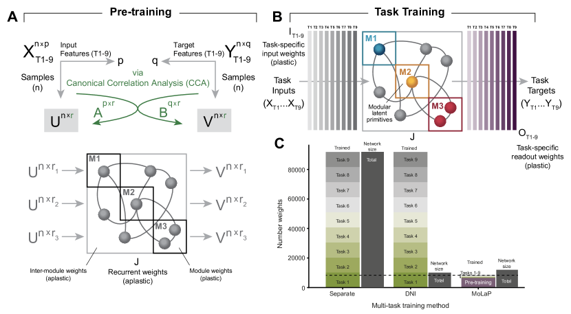
Modules are embedded within the larger network with module size $N^{M}\,=\,N^{Total}/{n^{M}}$, total number of units in the network $N^{Total}=100$, and number of modules $n^{M}=2$ throughout this paper. Modules are inter-connected with the reservoir, but not directly to each other (Figure 1A). Starting from an initial state, with weights drawn from a Gaussian distribution, each module is trained to produce a module-specific target output time series $\textbf{z}_{t}$ by minimizing the squared loss using the Adam optimizer (see A for more details). Module-specific inputs and targets are obtained via canonical correlation analysis (CCA; Figure 1A; see section 3.3).

In the pre-training phase (Figure 1A), intra-module weights are plastic (unfrozen) while inter-module weights remain aplastic (frozen). Modules are trained sequentially on latent primitives (see Section 3.3) such that only intra-module connections of the module currently being trained are allowed to change, while the others remain frozen. The gradient of the error, however, is computed across the whole network. Thus for the case outlined in Figure 1, for example, module 1 (M1) is trained first, followed by modules 2 (M2) and 3 (M3). When M1 is being trained, only connections inside of M1 are allowed to change, while the connections in the rest of the network remain frozen. After that, M1 connections are frozen, and M2’s intra-module connections are unfrozen for training.

3.2 Tasks

Neuroscience tasks [76], like the ones we employ here (explained in greater detail in A.1), are structured as trials, analogous to separate training batches. In each trial, stimuli are randomly drawn, e.g., from a distribution of possible orientations. In a given trial, there is an initial period without a stimulus in which animals are required to maintain fixation. Then, in the stimulus period, a stimulus appears for a given duration and the animal is again required to maintain fixation without responding. Finally, in the response period, the animal is allowed to make a response.

3.3 Deriving latent primitives

We derive inputs and targets for pre-training directly from the entire corpus of tasks by leveraging canonical correlation analysis (CCA; Figure 1A):

$$(\textbf{A}^{{}^{\prime}},\textbf{B}^{{}^{\prime}})\,=\,\operatorname*{argmax}_{\textbf{A},\textbf{B}}\,corr(\textbf{A}^{\intercal}\textbf{X}^{T1-9},\textbf{B}^{\intercal}\textbf{Y}^{T1-9})$$ (2)

$$\newline \textbf{U}_{n\,x\,r}\,=\,\textbf{A}^{{}^{\prime}\intercal}\textbf{X}\,\hskip 68.28644pt\,\textbf{V}_{n\,x\,r}\,=\,\textbf{B}^{{}^{\prime}\intercal}\textbf{Y}$$

In CCA, we seek A and B such that the correlation between the two variables X (task inputs) and Y (task outputs) is maximized. We then obtain the canonical variates U and V by projecting A and B back into the sample space of inputs and outputs, respectively, with $n$: number samples and $r$: number of latent dimensions. The canonical variates are used to pre-train the modules (3.1), with latent dimensions $r=1,2,3,..$ corresponding to module numbers $M=1,2,3,...$ (Figure 1A).

3.4 Task training

In the task-training phase (Figure 1B), recurrent weights remain aplastic (like in reservoir computing) and only input and output weights are allowed to change. Task-specific input ($\textbf{W}_{in}$) and readout weights ($\textbf{W}_{out}$) are trained by minimizing a task-specifc loss function (Eq 1). Separate linear readouts are used to obtain the outputs of the network (see A.2 for details):

$$\textbf{y}^{T1-9}_{t}\,=\,\textbf{W}^{T1-9}_{out}\textbf{h}^{M}_{t}$$ (3)

4 Results

Training multiple tasks with separate networks requires a high total number of parameters (as separate networks are used for each task) as well as a high number of parameter updates (as all of the network parameters are updated for each task). Thus, assuming a corpus of 9 tasks, a network size of 100 units, one input and one readout unit, naively training separate networks takes $9.18e5$ parameters and parameter updates (Table 1-Separate networks). In contrast, using recently proposed dynamical non-interference (DNI;[20]), one network is trained to perform all tasks; however, all of the parameters still need to be updated on each task as the shared representations are learned sequentially. Thus, DNI still requires $9.18e5$ parameters to be optimized (Table 1-DNI).

Similar to DNI, our approach (MoLaP) uses one network to perform all tasks; but MoLaP keeps both the total number of parameters, and the number of parameter updates low (Figure 1C-MoLaP). With MoLaP, the number of necessary parameter updates is $\sim 2$ orders of magnitude smaller compared to DNI and independent network approaches, with only a relatively modest $18\%$ increase in total parameter count compared to DNI (Figure 1C, Table 1). This arises from using shared reservoirs pre-trained on the joint statistics of the task corpus.

Table 1: Parameter count

Counts	Separate networks	DNI	MoLaP
Overall count	9.18e5	1.02e5	1.2e5
Number trained	9.18e5	9.18e5	5.2e3
Number trained per task	1.02e5	1.02e5	2e2

Fig 2: Performance comparison. Performance ($\%$ decisions correct on a $2000$-trial test set) shown for A. separately trained networks, B. a network trained with Dynamical non-interference (DNI), and C. with modular latent primitives (MoLaP). MoLaP performance is also compared to a version without pre-training (where all the connections in the reservoir remain frozen during pre-training) and to pre-training leveraging principal component analysis (PCA). Performance on task T7 for MoLaP with pre-training (D.) and without (E). Outputs vs Targets for output units 1 (D1/E1) and 2 (D2/E2), error (MSE) on 20 examples from the test set for output units 1 (D3/E3) and 2 (D4/E4), training loss (D5/E5), hidden units activity for a sample trial (D6/E6), recurrent weight matrix after training (D7/E7) and output weights after training (D8/E8). See A for further details.

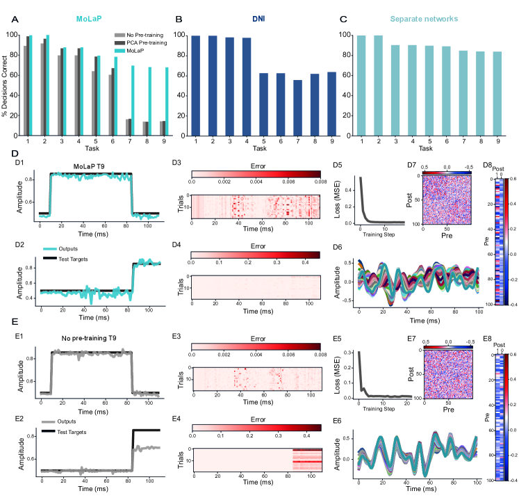
Despite low parameter update requirements, using MoLaP, we achieve similar performance to both independent networks and DNI (Figure 2), with successful learning ($>70\%$ decisions correct) across all 9 tasks (Figure 2A,B). To further investigate the role of latent primitive representations in MoLaP, we also compared a MoLaP version without pre-training (using randomly initialized modules like in reservoir computing), and a version using principal components analysis (PCA) instead of CCA to obtain latent inputs and targets for pre-training (Figure 2A). PCA offers an alternative way to derive latent primitives, and differs from CCA by successively maximizing the variance in the latent dimensions separately for inputs and outputs. The distinction is that PCA extracts a low-dimensional space from a single dataset (the covariance matrix), while CCA explicitly extracts modes that maximize variance across variables (the cross-covariance matrix; see also A for further details). This feature turns out to be crucial for deriving useful latent primitives.

Performance is more similar for easier tasks (T1-T4) than for more complex tasks (T5-T9), where flexible input-output mapping is required [19]. However, only MoLaP achieves the highest performance across all tasks. We show the performance of the trained MoLaP network with pre-training (Figure 2D) and without (Figure 2E) on task T7 (context-dependent memory task 1, see A.1 for task details). With pre-training, both readout variables hit the target (Figure 2Da-b) and decisions can be decoded correctly across the test set (Figure 2Dc-d), while in the version without pre-training, one of the readout variables misses the target (Figure 2Eb) and thus leads to incorrect decisions (Figure 2Ed).

4.1 Perturbations

Fig 3: Performance after modular perturbations. Performance ($\%$ decisions correct on a 2000 trial test set) after lesioning module 1 (M1) weights (A), module 2 (M2) weights (B), and inter-module weights (C). Performance as a function of percentage lesioned (a), with error bars showing the standard deviation of the mean across 30 random draws. MoLaP performance at $30\%$ weights lesioned (b-e), with outputs vs. targets for output units 1 (b) and 2 (c), and error (MSE) on 20 trials from the test set for output units 1 (d) and 2 (e). See A for further details.

Fig 4: Performance across all tasks. Performance ($\%$ decisions correct on a 2000 trial test set) as a function of percentage module 1 (M1) weights lesioned (A1), module 2 (M2) weights lesioned (A2), inter-module weights lesioned (A3), weights lesioned globally (B1), sigma of Gaussian noise added globally (B2, and percentage of units with activity silenced across the entire network (B3). Performance is computed across all nine tasks in the corpus

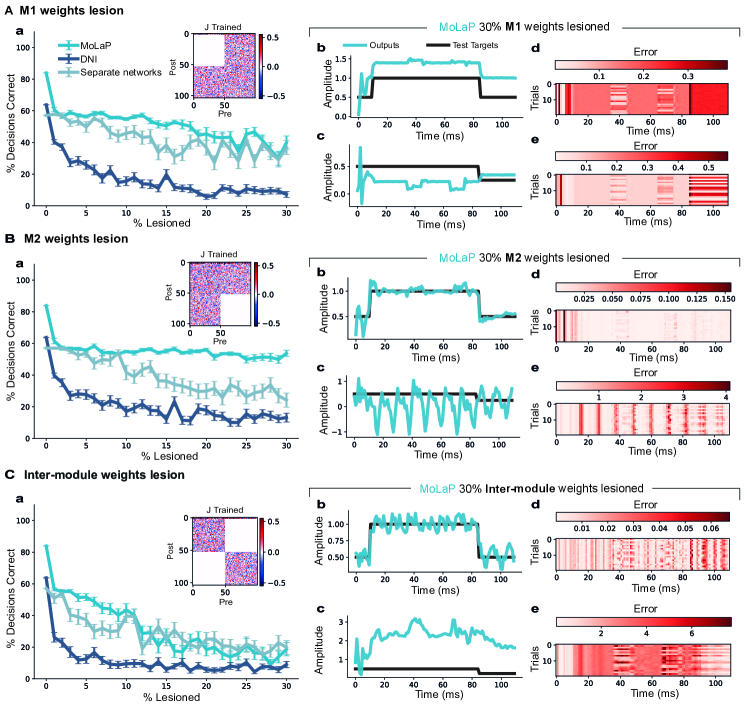
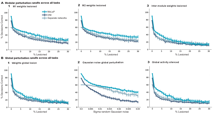
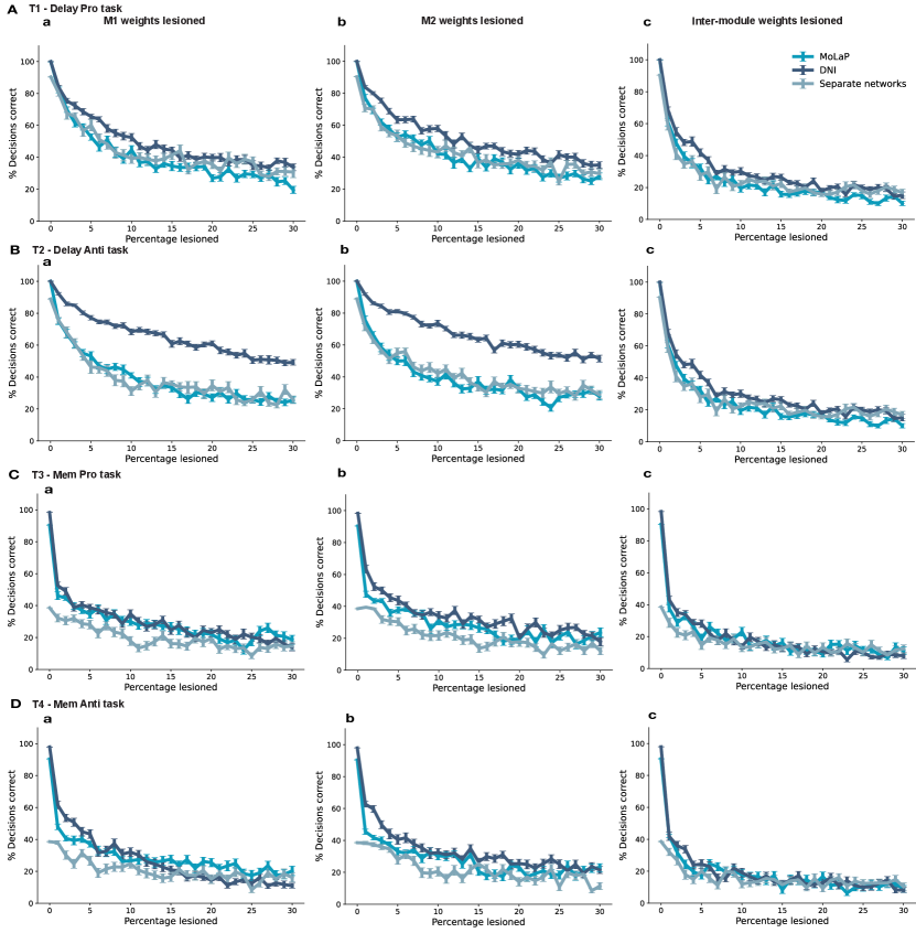
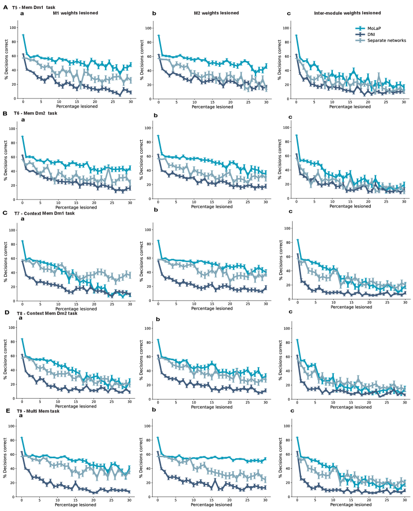
We analyzed performance after modular weight lesion for the different approaches, here shown for task T9 (Figure 3; see Figure S1&Figure S2 for a complete overview of tasks T1-T9)). Weights are ”lesioned" by picking a percentage of entries $W_{rec}^{i,j}$ from the connectivity matrix (Equation 1) and setting them to zero. With module 1 (M1) weights lesioned, MoLaP performance remained high when $<10\%$ of the intra-module weights were lesioned, above that of DNI and comparable to separately trained networks (Figure 3A). With module 2 (M2) weights lesioned, MoLaP performance remained high even at a higher percentage of intra-module weights lesioned, above that of DNI and separate networks (Figure 3B). When plotting outputs of MoLaP at $30\%$ of the M2 weights lesioned, we observed that the output signal of output unit 1 remained high, resulting in a higher percentage of correctly decoded decisions on average (Figure 3Bb,d) compared to when M1 was lesioned (Figure 3Ab,d). This can be explained by the fact that the first dimension of the canonical variables (on which M1 was trained) captures a higher percentage of the variance between inputs and targets than the second dimension (on which M2 was trained). Hence, when M2 is lesioned, M1 is still able to compensate and performance is preserved.

We also considered the effect of lesioning inter-module connections (Figure 3C). Performance degrades quickly when inter-weights are lesioned, for all approaches. When plotting outputs of MoLaP at $30\%$ inter-module connections lesioned, we observed that the combined error across output variables is higher compared to lesioning intra-module weights (Figure 3Cb-e). Based on this we would predict that cutting connections between areas is far more devastating than killing a few units within an area.

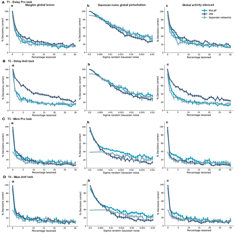
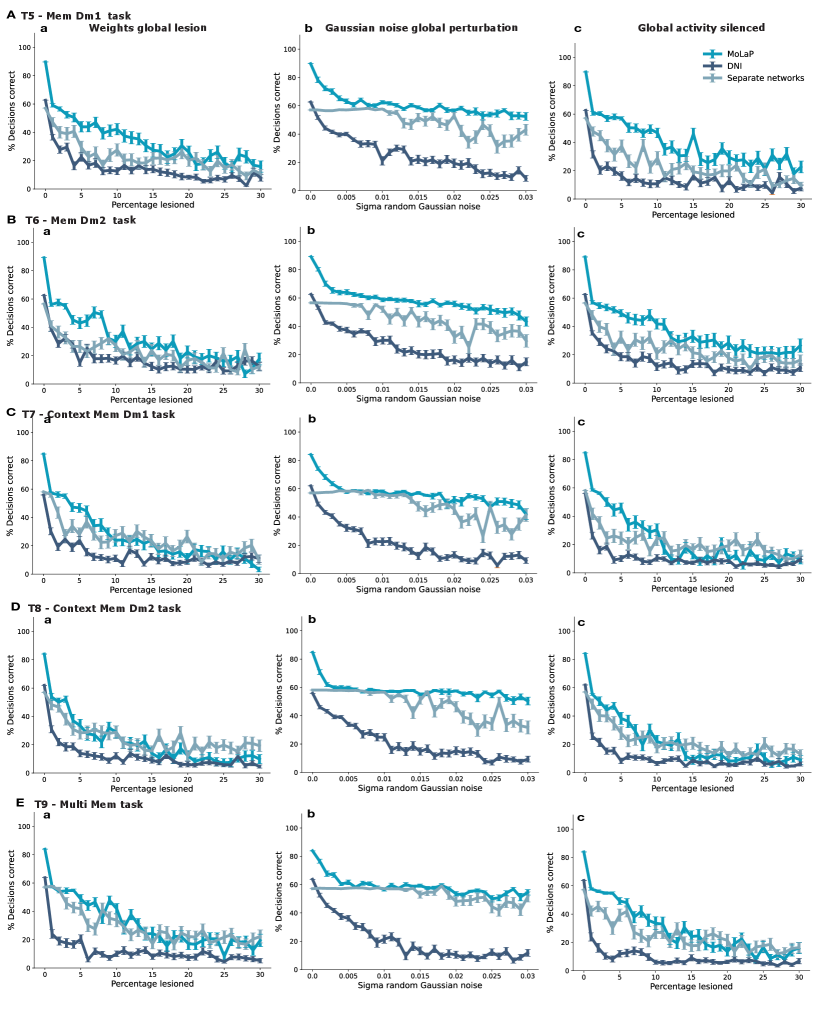
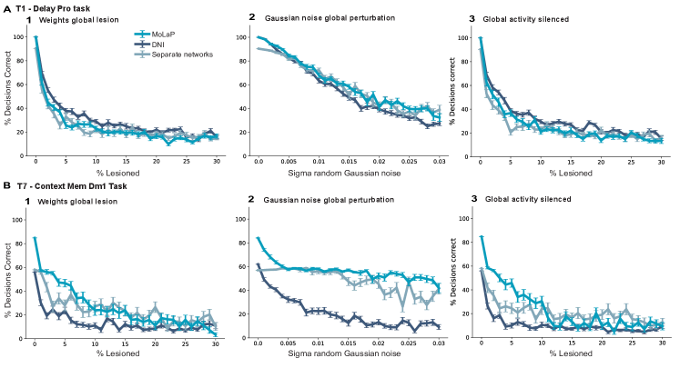
Furthermore, we analyzed performance after a number of different global perturbations (Figure S3,Figure S4,Figure S5). We considered three different global perturbations: lesioning entries in the connectivity matrix, adding global Gaussian noise to the entire connectivity matrix, and silencing activity of units in the network (by clamping their activity at zero). All perturbations are repeated for 30 random draws.

We found that on simpler tasks such as T1 (Figure S5A), all approaches perform similarly for the various global perturbations (see Figure S3&Figure S4 for all tasks). DNI performed somewhat better than the other approaches on simpler tasks when weights and activity were lesioned (Figure S5A,C), and somewhat worse than other approaches when noise was added globally (Figure S5B). On more complex tasks such as T7 (Figure S5B), however, we found that MoLaP was more robust to global perturbations. MoLaP performance remained higher compared to other approaches when up to $10\%$ of connections were lesioned (Figure S5Ba) or when up to $10\%$ of units were silenced (Figure 4Bc). MoLaP performance was also robust to global noise, even at relatively high levels (Figure S5Bb).

Fig 5: Generalization performance. Performance ($\%$ decisions correct on a $2000$-trial test set) for all tasks, after pre-training with CCA where all tasks were included (grey), pre-training with CCA where one task (dark blue) or two (light blue) tasks were left out, and pre-training with PCA where one task (dark green) or two tasks (light green) were left out. For leave-one-out, the left-out task corresponds to the task depicted on the x-axis. For leave-two-out, the task depicted and the one immediately next on the right were left out (in the case of T9, both T9 and T1 were left out).

Over the space of all the tasks we consider, we found that MoLaP performed better than the other approaches for all the perturbations under consideration (Figure 4).

4.2 Generalization

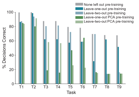
Finally, we analyzed the generalization performance of MoLaP by holding out each tasks, in turn, from the entire corpus used to derive the canonical variables for pre-training (Figure 5; see section 3 for details). We found that performance generalized to the left-out task relatively well, achieving higher performance than pre-training on the complete corpus using PCA (see Figure 2). We also observed some task-specific effects; performance on T7 was relatively worse when it was left out from the corpus of tasks used in pre-training, compared to when other tasks were left out. Even when two tasks were left out, MoLaP dynamics still generalized well with performance remaining high on the majority of tasks. See Appendix A for details on 2-tasks hold out protocol.

5 Discussion

We present a new approach for multi-task learning leveraging pre-trained modular latent primitives that act as inductive biases acquired through evolution or previous experience on shared statistics of a task corpus. The modules are inspired from organization of brain activity and provide useful dynamics for solving a number of different tasks; including those that are not in the corpus used for pre-training, but share some structure with it (i.e., generalization). We showed that our approach achieves high performance across all tasks, while not suffering from the effects of task order or task interference that might arise with other continual learning approaches [20, 81]. Crucially, our approach achieves high performance with $\sim 2$ orders of magnitude fewer parameter updates compared to other approaches (even including the pre-training phase) at the cost of only a moderate increase in the number of total parameters. MoLaP scales better with tasks, thus reducing overall training cost.

Our results also show that networks composed of pre-trained task modules are more robust to perturbations, even when perturbations are specifically targeted at particular modules. As readouts may draw upon dynamics across different modules, task performance is not drastically affected by the failure of any one particular module. The lower performance of the fully connected modular network may be due to the trained connection weights, which increase the inter-connectivity of different cell clusters and thus the susceptibility of local cell clusters to perturbations in distal parts of the network.

This result generates useful hypotheses for multi-task learning in the brain. It suggests that decision-making related circuits in the brain, such as in the prefrontal cortex, need not re-adjust all weights during learning. Rather, pre-existing dynamics may be leveraged to solve new tasks. This prediction could be tested by using recurrent networks fitted to population activity recorded from the brain [56, 50] as reservoirs of useful dynamics. We hypothesize that the fitted networks contain dynamics useful to new tasks; if so, it should be possible to train readout weights to perform new tasks. Moreover, targeted lesions may be performed to study the effect of perturbations on network dynamics in the brain; our work suggests networks with functional task modules are less prone to being disrupted by perturbations. Based on our work we would also expect functional modules to encode a set of basis-tasks (commonly occurring dynamics) for the purpose of solving future tasks.

In a recent study, [22] examined the effects of ’rich’ and ’lazy’ learning on acquired task representations and compared their findings to network representations in the brain of macaques and humans. The lazy learning paradigm is similar to ours in as far as learning is confined to readout weights; but it lacks our modular approach and does not show performance on multiple tasks. Conversely, our networks are not initialized with high variance weights as in the lazy regime. Ultimately, we observe improved robustness using our approach, unlike lazy learning which appears to confer lower robustness compared with rich learning.

This work enhances our understanding of resource-efficient continual learning in recurrent neural networks. As such, we do not anticipate any direct ethical or societal impact. Over the long-term, our work can have impact on related research communities such as neuroscience and deep learning, with societal impact depending on the development of these fields.

Appendix A Appendix

A.1 Tasks

We show that we can leverage our pre-configured modular network to learn a set of nine different neuroscience tasks, previously used to study multi-task learning [76, 20]. Trained simultaneously into one and the same network, these tasks produce a rich and varied population structure and are mapped into different parts of state space [76]. Simultaneous training, however, does not guarantee good performance on all tasks; this can be improved by using a multi-task training paradigm whereby new tasks are projected into non-interfering subspaces[20]. This approach is still dependent on task order, however: how well a new task is learnt often depends on its placement in the training curriculum.

We employ a set of nine different tasks: Delay Pro, Delay Anti, Mem Pro, Mem Anti, Mem Dm 1, Mem Dm 2, Context Mem Dm 1, Context Mem Dm 2 and Multi Mem. In Delay Pro and Delay Anti, the network receives three inputs (Fixation, cos($\theta$), sin($\theta$), with $\theta$ varying from 0-180 degrees). The angle inputs turned on at the Go-signal and remained on for the duration of the trial. The network was required to produce three outputs, yielding the correct location during the output period (when the fixation signal switched to zero). In the anti-versions, the network is required to respond in the direction opposite to the inputs. In Mem Pro and Mem Anti, the input stimulus turns off after a short, variable duration. As before, the network is required to produce three outputs encoding the correct location during the output period.

In Mem Dm 1 and Mem Dm 2, the network receives two inputs (Fixation, and a set of stimulus pulses separate by 100msec). The network is required to reproduce the higher valued pulse during the output period. Depending on the task, the network receives one or the other input stimulus pulse set.

In Context Mem Dm 1 and Context Mem Dm 2, the network receives three inputs (Fixation, and two sets of stimulus pulses). The network is required to reproduce the higher value pulse during the output period, ignoring the other input stimulus set. The two tasks differ in which input stimulus to pay attention to. In Multi Mem, the network again receives three inputs (Fixation, and both sets of stimulus pulses). The network needs to yield the summed value of the stimulus train with the higher total magnitude of the two pulses.

In models, a context signal indicates when to maintain fixation, separate inputs are fed in through different channels with dedicated input weights, and the choice can be indicated (and decoded) from separate output units for each target.

A.2 Training details

All networks were trained on a single laptop with the Apple M1 Max processor using a custom implementation of recurrent neural networks based on JAX [7]. The code to train MoLaP networks can be found at https://github.com/dashirn/MoLaP. We used a recurrent neural network (RNN) model with the hyperbolic tangent as the activation function throughout ($\sigma=\tanh$, Equation 1), in accordance with previous approaches to modeling neuroscience tasks [48, 10, 45]. Previous work suggests the dynamics obtained with different activation functions, such as $\tanh$ or $ReLu$, and different network models such as RNNs, GRUs and LSTMs are similar [43]. All networks were trained by minimizing the mean squared error using Adam as an optimizer. We used a custom implementation of DNI ([20]) leveraging the same setup as above based on JAX; we also compared our results with those obtained from the native implementation (available at https://github.com/LDlabs/seqMultiTaskRNN under a MIT license), and obtained similar results.

We performed a gridsearch over various parameter ranges (Table 2), and settled on the parameter combination that worked best across all training paradigms. We used a network of $N=100$ for MoLaP and separate networks, and $N=200$ for DNI.

Table 2: Parameter settings

Parameter	Parameter range considered
Network size	20 – 300
Learning rate	1e-3 – 1e-1
Batch size	20 – 400
Scaling factor $g$	1.1 – 1.8
$L2$-norm weight regularization parameter	5e-6 – 5e-5
Activity regularization parameter	1e-7
Number iterations before decreasing learning rate	100 – 300

A.2.1 Pre-training

The canonical correlation analysis (CCA) model was fitted to inputs and outputs across the entire corpus of tasks for the entire training set simultaneously, and then divided into separate batches for training. We found that two latent dimensions in the canonical variables ($U$ and $V$, see (2)) captured $\approx 60\%$ of the variance in the relationship between inputs and targets, while three captured $\approx 70\%$. We also fitted MoLaP networks with three modules and found they portrayed similarly to the results shown here with two modules.

For pre-training the recurrent network in MoLaP, we set the learning rate at $\alpha=3e-3$, with a batch size of 200 trials, the scaling factor at $g=1.5$, the $L2$-norm weight regularization parameter at 1e-5, the activity regularization parameter at 1e-7, and the number of iterations at 200. Each module was trained separately, with the number of units set at $N^{M1}=N^{M2}=50$. When a particular module was being trained, all other connections in the network remained frozen (information from the error gradient was prohibited from updating frozen units). So, for example, during training of module 1 (M1), all connections except those within module remained frozen. After M1 pre-training was complete, M1 connections were frozen M2 connections were unfrozen.

A.2.2 Pre-training with PCA

Alternatively, we also used principal components analysis (PCA) to derive inputs and outputs for pre-training. PCA was performed on the entire corpus of tasks for the entire training set simultaneously, separately for inputs and targets across all tasks. We thus obtained input and output vectors in the reduced space which we used analogously to CCA to train each module sequentially.

A.2.3 Task-training

In MoLaP, after pre-training, all connections in the recurrent weight matrix were frozen and only input and readout weights were allowed to change. Task-specific input and readout weights were trained for tasks T1-9.

For task-training in MoLaP, we set the learning rate at $\alpha=1e-2$ for all networks, the batch size at 200 trials, the scaling factor at $g=1.5$, the $L2$-norm weight regularization parameter at 1e-5, the activity regularization parameter at 1e-7, and the number of iterations at 200. Task-training in separate networks and with DNI only differed in that we set the learning rate at $\alpha=3e-3$ which we found worked best.

Across all approaches, the weights in the recurrent weight matrix, $\textbf{W}_{rec}$ (Equation 1), were initially drawn from the standard normal distribution and scaled by a factor of $\frac{g}{\sqrt{N}}$. The input weights, $\textbf{W}_{in}$, were also initially drawn from the standard normal distribution and scaled by a factor of $\frac{1}{\sqrt{N_{in}}}$ with $N_{in}$ varying by task. Each input unit also received an independent white noise input, $\boldsymbol{\eta}^{i}$, with zero mean and a standard deviation of $\sigma=0.002$. Output weights, $\textbf{W}_{out}$, were also initially drawn from the standard normal distribution and multiplied by a factor of $\frac{1}{\sqrt{N_{out}}}$ with $N_{out}$ varying by task.

A.3 Task performance

In order to measure task performance, a test set of 2000 trials was randomly generated from a separate random seed in JAX for each task. Performance was calculated as the percentage of correct decisions over this test set. Decisions, rather than other error metrics such as mean squared error, were chosen as a performance metric as they reflect the ultimate goal of biological agents. For all output units other than unit 1, a decision was considered correct if the mean output over the response period did not deviate more than a fixed amount ($\delta=0.1$) from the target direction. For output unit 1 (which indicated if fixation was maintained throughout the task), a deviation of ($\delta=0.1$) was permitted. For all output units, the response was decoded by taking the mean across the last 30 time points (response period) in a given trial. Performance was averaged across all output units.

A.4 Perturbation studies

We considered 3 types of perturbations: lesioned weights, silenced activity, and added Gaussian noise. In the case of lesioned weights, perturbations were performed both in a modular and in global fashion. In modular perturbations, connections to lesion were picked randomly from within modules only, or from among inter-modular connections (Figure S1,Figure S2). Global perturbations involved all the units in the network (Figure S3, Figure S4, Figure S5). Weight lesioning was performed by setting chosen connections to zero. Activity silencing was performed by silencing the activity of chosen units. Gaussian noise of different variance $\sigma\in[0,0.03]$ was added to the entire connectivity matrix. All perturbations were repeated for 30 different random draws.

A.5 Supplementary results

Fig S1: Performance after modular weight lesions (T1-T4). Performance (% decisions correct on a 250 trial test set) for tasks T1-T4

Fig S2: Performance after modular weight lesions (T5-T9). Performance (% decisions correct on a 250 trial test set) for tasks T1-T4 (MemDm1, MemDm2, ContextMemDm1, ContextMemDm2, MultiMem)

Fig S3: Performance after global perturbations (T1-T4). Performance (% decisions correct on a 250 trial test set) for tasks T1-T4 (MemDm1, MemDm2, ContextMemDm1, ContextMemDm2, MultiMem) as a function of % weights lesioned (A, E, I, M, Q), % units silenced (B, F, J, N, R),

Fig S4: Performance after global perturbations (T5-T9) Performance (% decisions correct on a 250 trial test set) for tasks T1-T4 (MemDm1, MemDm2, ContextMemDm1, ContextMemDm2, MultiMem)

Fig S5: Performance after global perturbations. Performance ($\%$ decisions correct on a 2000 trial test set) as a function of percentage weights lesioned globally (a), sigma of Gaussian noise added globally (b, and percentage of units with activity silenced (c), for task T1 (A) and task T7 (B). See A for further details.

References

- Adel et al. [2020] Tameem Adel, Han Zhao, and Richard E. Turner. Continual Learning with Adaptive Weights (CLAW). arXiv:1911.09514 [cs, stat], June 2020. URL http://arxiv.org/abs/1911.09514. arXiv: 1911.09514.
- Andreas et al. [2016] Jacob Andreas, Dan Klein, and Sergey Levine. Modular multitask reinforcement learning with policy sketches, 2016. URL https://arxiv.org/abs/1611.01796.
- Barak et al. [2013] Omri Barak, David Sussillo, Ranulfo Romo, Misha Tsodyks, and L F Abbott. From fixed points to chaos: Three models of delayed discrimination. Progress in Neurobiology, 103:214–222, March 2013. doi: 10.1016/j.pneurobio.2013.02.002. URL http://dx.doi.org/10.1016/j.pneurobio.2013.02.002. Publisher: Elsevier Ltd.
- Basile et al. [2020] Benjamin M. Basile, Victoria L. Templer, Regina Paxton Gazes, and Robert R. Hampton. Preserved visual memory and relational cognition performance in monkeys with selective hippocampal lesions. Sci. Adv., 6(29):eaaz0484, July 2020. ISSN 2375-2548. doi: 10.1126/sciadv.aaz0484. URL https://advances.sciencemag.org/lookup/doi/10.1126/sciadv.aaz0484.
- Billeh et al. [2014] Yazan N Billeh, Michael T Schaub, Costas A Anastassiou, Mauricio Barahona, and Christof Koch. Revealing cell assemblies at multiple levels of granularity. Journal of Neuroscience Methods, 236:92–106, October 2014. doi: 10.1016/j.jneumeth.2014.08.011. URL http://dx.doi.org/10.1016/j.jneumeth.2014.08.011. Publisher: Elsevier B.V.
- Botvinick et al. [2019] Matthew Botvinick, Sam Ritter, Jane X Wang, Zeb Kurth-Nelson, Charles Blundell, and Demis Hassabis. Reinforcement Learning, Fast and Slow. Trends in Cognitive Sciences, 23(5):408–422, May 2019. doi: 10.1016/j.tics.2019.02.006. URL https://doi.org/10.1016/j.tics.2019.02.006. Publisher: Elsevier Ltd.
- Bradbury et al. [2018] James Bradbury, Roy Frostig, Peter Hawkins, Matthew James Johnson, Chris Leary, Dougal Maclaurin, George Necula, Adam Paszke, Jake VanderPlas, Skye Wanderman-Milne, and Qiao Zhang. JAX: composable transformations of Python+NumPy programs, 2018. URL http://github.com/google/jax.
- Buonomano and Maass [2009] Dean V Buonomano and Wolfgang Maass. State-dependent computations: spatiotemporal processing in cortical networks. Nature Reviews Neuroscience, 10(2):113–125, January 2009. doi: 10.1038/nrn2558. URL http://www.nature.com/articles/nrn2558. Publisher: Nature Publishing Group.
- Carscadden et al. [2020] Kelly A. Carscadden, Nancy C. Emery, Carlos A. Arnillas, Marc W. Cadotte, Michelle E. Afkhami, Dominique Gravel, Stuart W. Livingstone, and John J. Wiens. Niche Breadth: Causes and Consequences for Ecology, Evolution, and Conservation. The Quarterly Review of Biology, 95(3):179–214, September 2020. ISSN 0033-5770, 1539-7718. doi: 10.1086/710388. URL https://www.journals.uchicago.edu/doi/10.1086/710388.
- Chaisangmongkon et al. [2017] Warasinee Chaisangmongkon, Sruthi K Swaminathan, David J Freedman, and Xiao-Jing Wang. Computing by Robust Transience: How the Fronto- Parietal Network Performs Sequential, Category- Based Decisions. Neuron, 93(6):1504–1517.e4, March 2017. doi: 10.1016/j.neuron.2017.03.002. URL http://dx.doi.org/10.1016/j.neuron.2017.03.002. Publisher: Elsevier Inc.
- Chen et al. [2021] Guang Chen, Byungwoo Kang, Jack Lindsey, Shaul Druckmann, and Nuo Li. Modularity and robustness of frontal cortical networks. Cell, 184(14):3717–3730.e24, 2021. ISSN 0092-8674. doi: https://doi.org/10.1016/j.cell.2021.05.026. URL https://www.sciencedirect.com/science/article/pii/S0092867421006565.
- Cossu et al. [2020] Andrea Cossu, Antonio Carta, and Davide Bacciu. Continual Learning with Gated Incremental Memories for sequential data processing. 2020 International Joint Conference on Neural Networks (IJCNN), pages 1–8, July 2020. doi: 10.1109/IJCNN48605.2020.9207550. URL http://arxiv.org/abs/2004.04077. arXiv: 2004.04077.
- Crawshaw [2020] Michael Crawshaw. Multi-task learning with deep neural networks: A survey, 2020. URL https://arxiv.org/abs/2009.09796.
- Csordás et al. [2020] Róbert Csordás, Sjoerd van Steenkiste, and Jürgen Schmidhuber. Are neural nets modular? inspecting functional modularity through differentiable weight masks, 2020. URL https://arxiv.org/abs/2010.02066.
- Curtis and D’Esposito [2004] C. E. Curtis and M. D’Esposito. The effects of prefrontal lesions on working memory performance and theory. Cognitive, Affective, & Behavioral Neuroscience, 4(4):528–539, December 2004. ISSN 1530-7026, 1531-135X. doi: 10.3758/CABN.4.4.528. URL http://link.springer.com/10.3758/CABN.4.4.528.
- Domenech and Koechlin [2015] Philippe Domenech and Etienne Koechlin. Executive control and decision-making in the prefrontal cortex. Current Opinion in Behavioral Sciences, 1:101–106, February 2015. doi: 10.1016/j.cobeha.2014.10.007. URL http://linkinghub.elsevier.com/retrieve/pii/S2352154614000278.
- Dominici et al. [2011] Nadia Dominici, Yuri P. Ivanenko, Germana Cappellini, Andrea d’Avella, Vito Mondì, Marika Cicchese, Adele Fabiano, Tiziana Silei, Ambrogio Di Paolo, Carlo Giannini, Richard E. Poppele, and Francesco Lacquaniti. Locomotor primitives in newborn babies and their development. Science, 334(6058):997–999, 2011. doi: 10.1126/science.1210617. URL https://www.science.org/doi/abs/10.1126/science.1210617.
- Draelos et al. [2017] Timothy J Draelos, Nadine E Miner, Christopher C Lamb, Jonathan A Cox, Craig M Vineyard, William M Severa, Conrad D James, and James B Aimone. Neurogenesis Deep Learning. IEEE, page 8, 2017.
- Dubreuil et al. [2021] Alexis Dubreuil, Adrian Valente, Manuel Beiran, Francesca Mastrogiuseppe, and Srdjan Ostojic. The role of population structure in computations through neural dynamics. bioRxiv, 2021. doi: 10.1101/2020.07.03.185942. URL https://www.biorxiv.org/content/early/2021/06/23/2020.07.03.185942.
- Duncker et al. [2020] Lea Duncker, Laura N Driscoll, Krishna V Shenoy, Maneesh Sahani, and David Sussillo. Organizing recurrent network dynamics by task-computation to enable continual learning. NeurIPS 2020, page 11, 2020.
- Finn et al. [2017] Chelsea Finn, Pieter Abbeel, and Sergey Levine. Model-agnostic meta-learning for fast adaptation of deep networks, 2017. URL https://arxiv.org/abs/1703.03400.
- Flesch et al. [2021] Timo Flesch, Keno Juechems, Tsvetomira Dumbalska, Andrew Saxe, and Christopher Summerfield. Rich and lazy learning of task representations in brains and neural networks. preprint, Neuroscience, April 2021. URL http://biorxiv.org/lookup/doi/10.1101/2021.04.23.441128.
- French [1999] Robert M. French. Catastrophic forgetting in connectionist networks. Trends in Cognitive Sciences, 3(4):128–135, 1999. ISSN 1364-6613. doi: https://doi.org/10.1016/S1364-6613(99)01294-2. URL https://www.sciencedirect.com/science/article/pii/S1364661399012942.
- Fu et al. [2015] Y. Fu, Y. Yu, G. Paxinos, C. Watson, and Z. Rusznák. Aging-dependent changes in the cellular composition of the mouse brain and spinal cord. Neuroscience, 290:406–420, April 2015. ISSN 03064522. doi: 10.1016/j.neuroscience.2015.01.039. URL https://linkinghub.elsevier.com/retrieve/pii/S0306452215000949.
- Golkar et al. [2019] Siavash Golkar, Michael Kagan, and Kyunghyun Cho. Continual Learning via Neural Pruning. arXiv:1903.04476 [cs, q-bio, stat], March 2019. URL http://arxiv.org/abs/1903.04476. arXiv: 1903.04476.
- Goulas et al. [2015] Alexandros Goulas, Alexander Schaefer, and Daniel S. Margulies. The strength of weak connections in the macaque cortico-cortical network. Brain Struct Funct, 220(5):2939–2951, September 2015. ISSN 1863-2653, 1863-2661. doi: 10.1007/s00429-014-0836-3. URL http://link.springer.com/10.1007/s00429-014-0836-3.
- Goyal et al. [2019] Anirudh Goyal, Alex Lamb, Jordan Hoffmann, Shagun Sodhani, Sergey Levine, Yoshua Bengio, and Bernhard Schölkopf. Recurrent independent mechanisms, 2019. URL https://arxiv.org/abs/1909.10893.
- Graves et al. [2014] Alex Graves, Greg Wayne, and Ivo Danihelka. Neural Turing Machines. arXiv:1410.5401 [cs], December 2014. URL http://arxiv.org/abs/1410.5401. arXiv: 1410.5401.
- Hadsell et al. [2020] Raia Hadsell, Dushyant Rao, Andrei A. Rusu, and Razvan Pascanu. Embracing Change: Continual Learning in Deep Neural Networks. Trends in Cognitive Sciences, 24(12):1028–1040, December 2020. ISSN 13646613. doi: 10.1016/j.tics.2020.09.004. URL https://linkinghub.elsevier.com/retrieve/pii/S1364661320302199.
- Henaff et al. [2016] Mikael Henaff, Jason Weston, Arthur Szlam, Antoine Bordes, and Yann LeCun. Tracking the world state with recurrent entity networks. 2016. doi: 10.48550/ARXIV.1612.03969. URL https://arxiv.org/abs/1612.03969.
- Hochreiter et al. [2001] Sepp Hochreiter, Yoshua Bengio, Paolo Frasconi, Jürgen Schmidhuber, et al. Gradient flow in recurrent nets: the difficulty of learning long-term dependencies, 2001.
- Hospedales et al. [2020] Timothy Hospedales, Antreas Antoniou, Paul Micaelli, and Amos Storkey. Meta-learning in neural networks: A survey, 2020. URL https://arxiv.org/abs/2004.05439.
- Jacobs et al. [1991] Robert A. Jacobs, Michael I. Jordan, Steven J. Nowlan, and Geoffrey E. Hinton. Adaptive mixtures of local experts. Neural Computation, 3(1):79–87, 1991. doi: 10.1162/neco.1991.3.1.79.
- Jaeger [2004] H. Jaeger. Harnessing Nonlinearity: Predicting Chaotic Systems and Saving Energy in Wireless Communication. Science, 304(5667):78–80, April 2004. ISSN 0036-8075, 1095-9203. doi: 10.1126/science.1091277. URL https://www.sciencemag.org/lookup/doi/10.1126/science.1091277.
- Kell et al. [2018] Alexander J.E. Kell, Daniel L.K. Yamins, Erica N. Shook, Sam V. Norman-Haignere, and Josh H. McDermott. A Task-Optimized Neural Network Replicates Human Auditory Behavior, Predicts Brain Responses, and Reveals a Cortical Processing Hierarchy. Neuron, 98(3):630–644.e16, May 2018. ISSN 08966273. doi: 10.1016/j.neuron.2018.03.044. URL https://linkinghub.elsevier.com/retrieve/pii/S0896627318302502.
- Kirkpatrick et al. [2017] James Kirkpatrick, Razvan Pascanu, Neil Rabinowitz, Joel Veness, Guillaume Desjardins, Andrei A. Rusu, Kieran Milan, John Quan, Tiago Ramalho, Agnieszka Grabska-Barwinska, Demis Hassabis, Claudia Clopath, Dharshan Kumaran, and Raia Hadsell. Overcoming catastrophic forgetting in neural networks. Proc Natl Acad Sci USA, 114(13):3521–3526, March 2017. ISSN 0027-8424, 1091-6490. doi: 10.1073/pnas.1611835114. URL http://www.pnas.org/lookup/doi/10.1073/pnas.1611835114.
- Koay et al. [2019] Sue Ann Koay, Adam S. Charles, Stephan Y. Thiberge, Carlos D. Brody, and David W. Tank. Sequential and efficient neural-population coding of complex task information. preprint, Neuroscience, October 2019. URL http://biorxiv.org/lookup/doi/10.1101/801654.
- Kveraga et al. [2007] Kestutis Kveraga, Avniel S Ghuman, and Moshe Bar. Top-down predictions in the cognitive brain. Brain and Cognition, 65(2):145–168, November 2007. doi: 10.1016/j.bandc.2007.06.007. URL http://linkinghub.elsevier.com/retrieve/pii/S0278262607000954.
- Lee et al. [2022] Sebastian Lee, Stefano Sarao Mannelli, Claudia Clopath, Sebastian Goldt, and Andrew Saxe. Maslow’s hammer for catastrophic forgetting: Node re-use vs node activation, 2022. URL https://arxiv.org/abs/2205.09029.
- Li et al. [2018] Shuai Li, Wanqing Li, Chris Cook, Ce Zhu, and Yanbo Gao. Independently recurrent neural network (indrnn): Building a longer and deeper rnn, 2018. URL https://arxiv.org/abs/1803.04831.
- Lopez-Paz and Ranzato [2017] David Lopez-Paz and Marc’Aurelio Ranzato. Gradient Episodic Memory for Continual Learning. arXiv:1706.08840 [cs], November 2017. URL http://arxiv.org/abs/1706.08840. arXiv: 1706.08840.
- Maass et al. [2002] Wolfgang Maass, Thomas Natschläger, and Henry Markram. Real-Time Computing Without Stable States: A New Framework for Neural Computation Based on Perturbations. Neural Computation, 14(11):2531–2560, November 2002. ISSN 0899-7667, 1530-888X. doi: 10.1162/089976602760407955. URL https://direct.mit.edu/neco/article/14/11/2531-2560/6650.
- Maheswaranathan et al. [2019] N Maheswaranathan, Alex H Williams, Matthew D Golub, Surya Ganguli, and David Sussillo. Universality and individuality in neural dynamics across large populations of recurrent networks. arXiv, pages 1–16, July 2019. URL https://arxiv.org/pdf/1907.08549.pdf.
- Mallya and Lazebnik [2017] Arun Mallya and Svetlana Lazebnik. Packnet: Adding multiple tasks to a single network by iterative pruning, 2017. URL https://arxiv.org/abs/1711.05769.
- Mante et al. [2013] Valerio Mante, David Sussillo, Krishna V Shenoy, and William T Newsome. Context-dependent computation by recurrent dynamics in prefrontal cortex. Nature, 503(7474):78–84, November 2013. ISSN 0028-0836. doi: 10.1038/nature12742. URL http://www.nature.com/doifinder/10.1038/nature12742.
- Meunier et al. [2010] David Meunier, Renaud Lambiotte, and Edward T. Bullmore. Modular and Hierarchically Modular Organization of Brain Networks. Front. Neurosci., 4, 2010. ISSN 1662-4548. doi: 10.3389/fnins.2010.00200. URL http://journal.frontiersin.org/article/10.3389/fnins.2010.00200/abstract.
- Murray et al. [2014] John D Murray, Alberto Bernacchia, David J Freedman, Ranulfo Romo, Jonathan D Wallis, Xinying Cai, Camillo Padoa-Schioppa, Tatiana Pasternak, Hyojung Seo, Daeyeol Lee, and Xiao-Jing Wang. A hierarchy of intrinsic timescales across primate cortex. Nat Neurosci, 17(12):1661–1663, December 2014. ISSN 1097-6256, 1546-1726. doi: 10.1038/nn.3862. URL http://www.nature.com/articles/nn.3862.
- Márton et al. [2020] Christian D. Márton, Simon R. Schultz, and Bruno B. Averbeck. Learning to select actions shapes recurrent dynamics in the corticostriatal system. Neural Networks, 132:375–393, December 2020. ISSN 08936080. doi: 10.1016/j.neunet.2020.09.008. URL https://linkinghub.elsevier.com/retrieve/pii/S0893608020303312.
- Nichol et al. [2018] Alex Nichol, Joshua Achiam, and John Schulman. On first-order meta-learning algorithms, 2018. URL https://arxiv.org/abs/1803.02999.
- Pandarinath et al. [2018] Chethan Pandarinath, Daniel J. O’Shea, Jasmine Collins, Rafal Jozefowicz, Sergey D. Stavisky, Jonathan C. Kao, Eric M. Trautmann, Matthew T. Kaufman, Stephen I. Ryu, Leigh R. Hochberg, Jaimie M. Henderson, Krishna V. Shenoy, L. F. Abbott, and David Sussillo. Inferring single-trial neural population dynamics using sequential auto-encoders. Nat Methods, 15(10):805–815, October 2018. ISSN 1548-7091, 1548-7105. doi: 10.1038/s41592-018-0109-9. URL http://www.nature.com/articles/s41592-018-0109-9.
- Parisi et al. [2019] German I. Parisi, Ronald Kemker, Jose L. Part, Christopher Kanan, and Stefan Wermter. Continual lifelong learning with neural networks: A review. Neural Networks, 113:54–71, May 2019. ISSN 08936080. doi: 10.1016/j.neunet.2019.01.012. URL https://linkinghub.elsevier.com/retrieve/pii/S0893608019300231.
- Pateria et al. [2021] Shubham Pateria, Budhitama Subagdja, Ah-hwee Tan, and Chai Quek. Hierarchical reinforcement learning: A comprehensive survey. ACM Comput. Surv., 54(5), jun 2021. ISSN 0360-0300. doi: 10.1145/3453160. URL https://doi.org/10.1145/3453160.
- Pathak et al. [2018] Jaideep Pathak, Brian Hunt, Michelle Girvan, Zhixin Lu, and Edward Ott. Model-Free Prediction of Large Spatiotemporally Chaotic Systems from Data: A Reservoir Computing Approach. Phys. Rev. Lett., 120(2):024102, January 2018. ISSN 0031-9007, 1079-7114. doi: 10.1103/PhysRevLett.120.024102. URL https://link.aps.org/doi/10.1103/PhysRevLett.120.024102.
- Pearl [2009] Judea Pearl. Causality: Models, Reasoning and Inference. Cambridge University Press, USA, 2nd edition, 2009. ISBN 052189560X.
- Perich and Rajan [2020] Matthew G Perich and Kanaka Rajan. Rethinking brain-wide interactions through multi-region ‘network of networks’ models. Current Opinion in Neurobiology, 65:146–151, December 2020. ISSN 09594388. doi: 10.1016/j.conb.2020.11.003. URL https://linkinghub.elsevier.com/retrieve/pii/S0959438820301707.
- Perich et al. [2020] Matthew G. Perich, Charlotte Arlt, Sofia Soares, Megan E. Young, Clayton P. Mosher, Juri Minxha, Eugene Carter, Ueli Rutishauser, Peter H. Rudebeck, Christopher D. Harvey, and Kanaka Rajan. Inferring brain-wide interactions using data-constrained recurrent neural network models. preprint, Neuroscience, December 2020. URL http://biorxiv.org/lookup/doi/10.1101/2020.12.18.423348.
- Power et al. [2011] Jonathan D. Power, Alexander L. Cohen, Steven M. Nelson, Gagan S. Wig, Kelly Anne Barnes, Jessica A. Church, Alecia C. Vogel, Timothy O. Laumann, Fran M. Miezin, Bradley L. Schlaggar, and Steven E. Petersen. Functional Network Organization of the Human Brain. Neuron, 72(4):665–678, November 2011. ISSN 08966273. doi: 10.1016/j.neuron.2011.09.006. URL https://linkinghub.elsevier.com/retrieve/pii/S0896627311007926.
- Rajan et al. [2016] Kanaka Rajan, Christopher D Harvey, and David W Tank. Recurrent Network Models of Sequence Generation and Memory. Neuron, 90(1):128–142, April 2016. doi: 10.1016/j.neuron.2016.02.009. URL http://dx.doi.org/10.1016/j.neuron.2016.02.009. Publisher: Elsevier Inc.
- Ramasesh et al. [2020] Vinay V. Ramasesh, Ethan Dyer, and Maithra Raghu. Anatomy of catastrophic forgetting: Hidden representations and task semantics, 2020. URL https://arxiv.org/abs/2007.07400.
- Remington et al. [2018] Evan D. Remington, Seth W. Egger, Devika Narain, Jing Wang, and Mehrdad Jazayeri. A Dynamical Systems Perspective on Flexible Motor Timing. Trends in Cognitive Sciences, 22(10):938–952, October 2018. ISSN 13646613. doi: 10.1016/j.tics.2018.07.010. URL https://linkinghub.elsevier.com/retrieve/pii/S1364661318301724.
- Richards et al. [2019] Blake A Richards, Timothy P Lillicrap, Philippe Beaudoin, Yoshua Bengio, Rafal Bogacz, Amelia Christensen, Claudia Clopath, Rui Ponte Costa, Archy Berker, Surya Ganguli, Colleen J Gillon, Danijar Hafner, Adam Kepecs, Nikolaus Kriegeskorte, Peter Latham, Grace W Lindsay, Kenneth D Miller, Richard Naud, Christopher C Pack, Panayiota Poirazi, Pieter Roelfsema, João Sacramento, Andrew Saxe, Benjamin Scellier, Anna C Schapiro, Walter Senn, Greg Wayne, Daniel Yamins, Friedemann Zenke, Joel Zylberberg, Denis Therien, and Konrad P Kording. A deep learning framework for neuroscience. Nature Neuroscience, 22(11):1–10, October 2019. doi: 10.1038/s41593-019-0520-2. URL http://dx.doi.org/10.1038/s41593-019-0520-2. Publisher: Springer US.
- Rosenbaum et al. [2019] Clemens Rosenbaum, Ignacio Cases, Matthew Riemer, and Tim Klinger. Routing networks and the challenges of modular and compositional computation, 2019. URL https://arxiv.org/abs/1904.12774.
- Rusu et al. [2016] Andrei A. Rusu, Neil C. Rabinowitz, Guillaume Desjardins, Hubert Soyer, James Kirkpatrick, Koray Kavukcuoglu, Razvan Pascanu, and Raia Hadsell. Progressive Neural Networks. arXiv:1606.04671 [cs], September 2016. URL http://arxiv.org/abs/1606.04671. arXiv: 1606.04671.
- Sakai [2008] Katsuyuki Sakai. Task Set and Prefrontal Cortex. Annual Review of Neuroscience, 31(1):219–245, July 2008. doi: 10.1146/annurev.neuro.31.060407.125642. URL http://www.annualreviews.org/doi/10.1146/annurev.neuro.31.060407.125642.
- Santoro et al. [2018] Adam Santoro, Ryan Faulkner, David Raposo, Jack Rae, Mike Chrzanowski, Theophane Weber, Daan Wierstra, Oriol Vinyals, Razvan Pascanu, and Timothy Lillicrap. Relational recurrent neural networks, 2018. URL https://arxiv.org/abs/1806.01822.
- Schwarz et al. [2018] Jonathan Schwarz, Jelena Luketina, Wojciech M Czarnecki, Agnieszka Grabska-Barwinska, Yee Whye Teh, Razvan Pascanu, and Raia Hadsell. Progress & Compress: A scalable framework for continual learning. PMLR, 80:10, 2018.
- Serrà et al. [2018] Joan Serrà, Dídac Surís, Marius Miron, and Alexandros Karatzoglou. Overcoming Catastrophic Forgetting with Hard Attention to the Task. PMLR, 80:10, 2018.
- Sporns and Betzel [2016] Olaf Sporns and Richard F. Betzel. Modular Brain Networks. Annu. Rev. Psychol., 67(1):613–640, January 2016. ISSN 0066-4308, 1545-2085. doi: 10.1146/annurev-psych-122414-033634. URL http://www.annualreviews.org/doi/10.1146/annurev-psych-122414-033634.
- Sussillo and Abbott [2009] David Sussillo and L F Abbott. Generating Coherent Patterns of Activity from Chaotic Neural Networks. Neuron, 63(4):544–557, August 2009. doi: 10.1016/j.neuron.2009.07.018. URL http://dx.doi.org/10.1016/j.neuron.2009.07.018. Publisher: Elsevier Ltd.
- Sussillo and Barak [2013] David Sussillo and Omri Barak. Opening the Black Box: Low-Dimensional Dynamics in High-Dimensional Recurrent Neural Networks. Neural Computation, pages 1–24, January 2013. doi: https://doi.org/10.1162/NECO_a_00409. URL https://www.mitpressjournals.org/doi/pdf/10.1162/NECO_a_00409.
- Sussillo et al. [2015] David Sussillo, Mark M Churchland, Matthew T Kaufman, and Krishna V Shenoy. A neural network that finds a naturalistic solution for the production of muscle activity. Nature Neuroscience, 18(7):1025–1033, June 2015. doi: 10.1038/nn.4042. URL http://www.nature.com/articles/nn.4042. Publisher: Nature Publishing Group.
- Vincent-Lamarre et al. [2016] Philippe Vincent-Lamarre, Guillaume Lajoie, and Jean-Philippe Thivierge. Driving reservoir models with oscillations: a solution to the extreme structural sensitivity of chaotic networks. J Comput Neurosci, 41(3):305–322, December 2016. ISSN 0929-5313, 1573-6873. doi: 10.1007/s10827-016-0619-3. URL http://link.springer.com/10.1007/s10827-016-0619-3.
- Wang et al. [2018] Jane X. Wang, Zeb Kurth-Nelson, Dharshan Kumaran, Dhruva Tirumala, Hubert Soyer, Joel Z. Leibo, Demis Hassabis, and Matthew Botvinick. Prefrontal cortex as a meta-reinforcement learning system. bioRxiv, 2018. doi: 10.1101/295964. URL https://www.biorxiv.org/content/early/2018/04/13/295964.
- Wang and Kennedy [2016] Xiao-Jing Wang and Henry Kennedy. Brain structure and dynamics across scales: in search of rules. Current Opinion in Neurobiology, 37:92–98, April 2016. ISSN 09594388. doi: 10.1016/j.conb.2015.12.010. URL https://linkinghub.elsevier.com/retrieve/pii/S0959438815001889.
- Westlye et al. [2010] L. T. Westlye, K. B. Walhovd, A. M. Dale, A. Bjornerud, P. Due-Tonnessen, A. Engvig, H. Grydeland, C. K. Tamnes, Y. Ostby, and A. M. Fjell. Life-Span Changes of the Human Brain White Matter: Diffusion Tensor Imaging (DTI) and Volumetry. Cerebral Cortex, 20(9):2055–2068, September 2010. ISSN 1047-3211, 1460-2199. doi: 10.1093/cercor/bhp280. URL https://academic.oup.com/cercor/article-lookup/doi/10.1093/cercor/bhp280.
- Yang et al. [2018] Guangyu Robert Yang, Madhura R Joglekar, H Francis Song, William T Newsome, and Xiao-Jing Wang. Task representations in neural networks trained to perform many cognitive tasks. Nature Neuroscience, 22(2):1–16, December 2018. doi: 10.1038/s41593-018-0310-2. URL http://dx.doi.org/10.1038/s41593-018-0310-2. Publisher: Springer US.
- Yoon et al. [2018] Jaehong Yoon, Eunho Yang, Jeongtae Lee, and Sung Ju Hwang. Lifelong learning with dynamically expandable networks. ICLR, page 11, 2018.
- Yu et al. [2020] Tianhe Yu, Saurabh Kumar, Abhishek Gupta, Sergey Levine, Karol Hausman, and Chelsea Finn. Gradient Surgery for Multi-Task Learning. arXiv:2001.06782 [cs, stat], December 2020. URL http://arxiv.org/abs/2001.06782. arXiv: 2001.06782.
- Zador [2019] Anthony M Zador. A critique of pure learning and what artificial neural networks can learn from animal brains. Nature Communications, 10(1):1–7, August 2019. doi: 10.1038/s41467-019-11786-6. URL http://dx.doi.org/10.1038/s41467-019-11786-6. Publisher: Springer US.
- Zeng et al. [2018] Guanxiong Zeng, Yang Chen, Bo Cui, and Shan Yu. Continuous Learning of Context-dependent Processing in Neural Networks. arXiv:1810.01256 [cs], October 2018. URL http://arxiv.org/abs/1810.01256. arXiv: 1810.01256.
- Zenke et al. [2017] Friedemann Zenke, Ben Poole, and Surya Ganguli. Continual Learning Through Synaptic Intelligence. arXiv:1703.04200 [cs, q-bio, stat], June 2017. URL http://arxiv.org/abs/1703.04200. arXiv: 1703.04200.