Abstract.

We provide a sharp lower bound on the $p$-norm of a sum of independent uniform random variables in terms of its variance when $0<p<1$. We address an analogous question for $p$-Rényi entropy for $p$ in the same range.

2020 Mathematics Subject Classification. Primary 60E15; Secondary 26D15.

Key words. Sharp moment comparison, Khinchin inequalities, Sums of independent random variables, Uniform random variables, Rényi entropy.

1. Introduction and results

Moment comparison inequalities for sums of independent random variables, that is Khinchin-type inequalities, first established by Khinchin for Rademacher random variables (random signs) in his proof of the law of the iterated logarithm (see [14]), have been extensively studied ever since his work. Particularly challenging, interesting and conducive to new methods is the question of sharp constants in such inequalities. We only mention in passing several classical as well as recent references, [1, 9, 11, 15, 17, 18, 23, 26]. This paper finishes the pursuit of sharp constants in $L_{p}-L_{2}$ Khinchin inequalities for sums of independent uniform random variables, addressing the range $0<p<1$. We are also concerned with a $p$-Rényi entropy analogue.

1.1. Moments

Let $U_{1},U_{2},\dots$ be independent random variables uniform on $[-1,1]$. As usual, $\|X\|_{p}=(\mathbb{E}|X|^{p})^{1/p}$ is the $p$-norm of a random variable $X$. Given $p>-1$, let $c_{p}$ and $C_{p}$ be the best constants such that for every integer $n\geqslant 1$ and real numbers $a_{1},\dots,a_{n}$, we have

(1) $$c_{p}\left(\sum_{j=1}^{n}a_{j}^{2}\right)^{1/2}\leqslant\left\|\sum_{j=1}^{n}a_{j}U_{j}\right\|_{p}\leqslant C_{p}\left(\sum_{j=1}^{n}a_{j}^{2}\right)^{1/2},$$

or in other words, since $\|\sum a_{j}U_{j}\|_{2}={\sqrt{\operatorname{Var}(\sum a_{j}U_{j})}}=3^{-1/2}\left(\sum a_{j}^{2}\right)^{1/2}$, finding $c_{p}$ and $C_{p}$ amounts to extremising the $p$-norm of the sum $\sum a_{j}U_{j}$ subject to a fixed variance,

$$c_{p}=\inf\left\|\sum_{j=1}^{n}a_{j}U_{j}\right\|_{p},\qquad C_{p}=\sup\left\|\sum_{j=1}^{n}a_{j}U_{j}\right\|_{p},$$

where the infimum and supremum and taken over all integers $n\geqslant 1$ and unit vectors $a=(a_{1},\dots,a_{n})$ in $\mathbb{R}^{n}$.

For $p>1$, the optimal constants $c_{p},C_{p}$ were found by Latała and Oleszkiewicz in [19] (see also [8] for an alternative approach and [1, 16] for generalisations in higher dimensions). They read

(2) $$\begin{split}c_{p}&=\|U_{1}\|_{p}=(1+p)^{-1/p},\\ C_{p}&=\lim_{n\to\infty}\left\|\frac{U_{1}+\dots+U_{n}}{\sqrt{n}}\right\|_{p}=\|Z\|_{p}/\sqrt{3},\quad p>1,\end{split}$$

where $Z$ here and throughout the text denotes a standard $N(0,1)$ Gaussian random variable. In fact stronger results are available (extremisers are known via Schur-convexity for each fixed $n$).

For $-1<p<0$, the behaviour is complicated by a phase transition (similar to the case of random signs as established by Haagerup in [9]). It has recently been proved in [4] that

$$c_{p} =\min\left\{\|Z\|_{p}/\sqrt{3},\left\|U_{1}+U_{2}\right\|_{p}/\sqrt{2}\right\}=\begin{cases}\|Z\|_{p}/\sqrt{3},&-0.793..<p<0,\\ \left\|U_{1}+U_{2}\right\|_{p}/\sqrt{2},&-1<p{\leqslant}-0.793..,\end{cases}$$

and the limiting behaviour of $c_{p}$ as $p\to-1^{+}$ recovers Ball’s celebrated cube slicing inequality from [2].

The fact that

$$C_{p}=\|U_{1}\|_{p},\qquad-1<p<1,$$

follows easily from unimodality and Jensen’s inequality (see, e.g. Proposition 15 in [8]).

Thus what is unknown is the optimal value of $c_{p}$ for $0<p<1$ and this paper fills out this gap. Our main result reads as follows.

Theorem 1.

For $0<p<1$, $c_{p}=\|Z\|_{p}/\sqrt{3}$ is the best constant in (1).

We record for future use that

$$\|Z\|_{p}^{p}=\frac{1}{\sqrt{2\pi}}\int_{-\infty}^{\infty}|x|^{p}e^{-x^{2}/2}\mathrm{d}x=\frac{2^{p/2}}{\sqrt{\pi}}\Gamma\left(\frac{1+p}{2}\right).$$

1.2. Rényi entropy

For $p\in[0,\infty]$, the $p$-Rényi entropy of a random variable $X$ with density $f$ is defined as (see [25]),

$$h_{p}(X)=\frac{1}{1-p}\log\left(\int_{\mathbb{R}}f^{p}\right)$$

with $p\in\{0,1,\infty\}$ defined by taking the limit: $h_{0}(f)=\log|\text{supp}(f)|$ is the logarithm of the Lebesgue measure of the support of $f$, $h_{1}(f)=-\int f\log f$ is the Shannon entropy, and $h_{\infty}=-\log\|f\|_{\infty}$, where $\|f\|_{\infty}$ is the $\infty$-norm of $f$ (with respect to Lebesgue measure). The question of maximising Rényi entropy under a variance constraint (or more generally, a moment constraint) for general distributions has been fully understood and leads to the notion of relative entropy that is of importance in information theory, providing a natural way of measuring distance to the extremal distributions (see [5, 13, 20, 22]). In analogy to Theorem 1, we provide an answer for $p$-Rényi entropies, $0<p<1$, for sums of uniforms under the variance constraints.

Theorem 2.

Let $0<p<1$. For every unit vector $a=(a_{1},\dots,a_{n})$, we have

$$h_{p}\left(U_{1}\right)\leqslant h_{p}\left(\sum_{j=1}^{n}a_{j}U_{j}\right)\leqslant h_{p}\left(Z/\sqrt{3}\right).$$

The lower bound is a simple consequence of the entropy power inequality. The upper bound is interesting in that the maximizer among all distributions of fixed variance is not Gaussian (rather, with density proportional to $(1+x^{2})^{-1/(1-p)}$ for $\frac{1}{3}<p<1$ and it does not exist for $p<\frac{1}{3}$, see e.g. [5]). It is derived from the $L_{q}-L_{2}$ Khinchin inequality for even $q$.

1.3. Organisation of the paper

In Section 2 we give an overview of the proof of Theorem 1 and show a reduction to two main steps: an integral inequality and an inductive argument. Then in Section 3 we gather all technical lemmas needed to accomplish these steps which is then done in Sections 4 and 5, respectively. Section 6 contains a short proof of Theorem 2.

Acknowledgments.

We should very much like to thank Alexandros Eskenazis for the stimulating correspondence. We are also indebted to anonymous referees for many valuable comments which helped significantly improve the manuscript.

2. Proof of the main result

2.1. Overview

We follow an approach developed by Haagerup in [9], with major simplifications advanced later by Nazarov and Podkorytov in [24]. In essence, the argument begins with a Fourier-analytic integral representation for the power function $|\cdot|^{p}$ which allows to take advantage of independence and in turn, by virtue of the AM-GM inequality, to reduce the problem to establishing a certain integral inequality involving the Fourier transforms of the uniform and Gaussian distributions. Since this inequality holds only in a specific range of parameters, additional arguments are needed, mainly an induction on the number of summands $n$ (similar problems were faced in e.g. [4, 24, 15]). In our case, this is further complicated by the fact that the base of the induction fails for large values of $p$ (roughly for $p>0.7$).

Remark 3.

We point out that the main difference between the regimes $p{\geqslant}1$ and $p<1$ is that for the former convexity type arguments allow to establish stronger comparison results, namely the Schur-convexity/concavity of the function

$$(\sqrt{x_{1}},\dots,\sqrt{x_{n}})\mapsto\mathbb{E}\left|\sum_{j=1}^{n}\sqrt{x_{j}}U_{j}\right|^{p}.$$

By combining Theorems 2 and 3 of [1] (see also (6.1) therein), a necessary condition for this is the concavity/convexity of the function $x\mapsto\mathbb{E}|U_{1}+\sqrt{x}|^{p}$. The calculations following Corollary 1 in the same work show that this is the case only for $p\geqslant 1$. In other words, when $p<1$, the function above is neither Schur-convex nor Schur-concave and the Fourier-analytic approach seems to be indispensable.

2.2. Details

The aforementioned Fourier-analytic formula reads as follows (it can be found for instance in [9], but we sketch its proof for completeness).

Lemma 4.

Let $0<p<2$ and $\kappa_{p}=\frac{2}{\pi}\Gamma(1+p)\sin\left(\frac{\pi p}{2}\right)$. For a random variable $X$ in $L_{2}$ with characteristic function $\phi_{X}(t)=\mathbb{E}e^{itX}$, we have

$$\mathbb{E}|X|^{p}=\kappa_{p}\int_{0}^{\infty}\frac{1-\mathrm{Re}\phi_{X}(t)}{t^{p+1}}\mathrm{d}t.$$

Proof.

A change of variables establishes $|x|^{p}=\kappa_{p}\int_{0}^{\infty}\frac{1-\cos(tx)}{t^{p+1}}\mathrm{d}t$, $x\in\mathbb{R}$. We then apply this to $X$ and take the expectation. ∎

We begin the proof of Theorem 1. Let $0<p<1$ and $c_{p}=\|Z\|_{p}/\sqrt{3}$. Let $a_{1},\dots,a_{n}$ be (without loss of generality) nonzero real numbers with $\sum_{j=1}^{n}a_{j}^{2}=1$. By symmetry of the uniform distribution we assume without loss of generality that they are in fact positive. From Lemma 4, we obtain

$$\mathbb{E}\left|\sum_{j=1}^{n}a_{j}U_{j}\right|^{p}=\kappa_{p}\int_{0}^{\infty}\frac{1-\prod_{j=1}^{n}\phi(a_{j}t)}{t^{1+p}}\mathrm{d}t,$$

where we have used independence and put $\phi(t)=\mathbb{E}e^{itU_{1}}=\frac{\sin t}{t}$ to be the characteristic function of the uniform distribution. We seek a sharp lower-bound on this expression (attained when $a_{1}=\dots=a_{n}=\frac{1}{\sqrt{n}}$ and $n\to\infty$, as anticipated by Theorem 1). By the AM-GM inequality,

$$\left|\prod_{j=1}^{n}\phi(a_{j}t)\right|\leqslant\sum_{j=1}^{n}a_{j}^{2}|\phi(a_{j}t)|^{1/a_{j}^{2}}.$$

As a result,

$$\mathbb{E}\left|\sum_{j=1}^{n}a_{j}U_{j}\right|^{p}\geqslant\sum_{j=1}^{n}a_{j}^{2}\mathcal{I}_{p}(1/a_{j}^{2}),$$

where we have set

$$\mathcal{I}_{p}(s)=\kappa_{p}\int_{0}^{\infty}\frac{1-\left|\frac{\sin(t/\sqrt{s})}{t/\sqrt{s}}\right|^{s}}{t^{p+1}}\mathrm{d}t,\qquad s\geqslant 1.$$

Note that $\frac{\sin(t/\sqrt{s})}{t/\sqrt{s}}=1-\frac{t^{2}}{6s}+O(1/s^{2})$ for a fixed $t$ as $s\to\infty$ and consequently,

$$\mathcal{I}_{p}(\infty)=\lim_{s\to\infty}\mathcal{I}_{p}(s)=\kappa_{p}\int_{0}^{\infty}\frac{1-e^{-t^{2}/6}}{t^{p+1}}\mathrm{d}t=\mathbb{E}|Z/\sqrt{3}|^{p},$$

where the last equality follows from Lemma 4 because $e^{-t^{2}/6}$ is the characteristic function of $Z/\sqrt{3}$, $Z\sim N(0,1)$ (the exchange of the order of the limit and integration in the second equality can be easily justified by truncating the integral, see, e.g., (15) in [4]). In particular, if for some $p$ and $s_{0}$,

(3) $$\mathcal{I}_{p}(s)\geqslant\mathcal{I}_{p}(\infty),\qquad\text{for all }s\geqslant s_{0},$$

then

(4) $$\mathbb{E}\left|\sum_{j=1}^{n}a_{j}U_{j}\right|^{p}\geqslant\mathbb{E}|Z/\sqrt{3}|^{p}=c_{p}^{p},$$

as long as $1/a_{j}^{2}\geqslant s_{0}$ for each $j$. If (3) were true for all $0<p<1$ with $s_{0}=1$, then the proof of Theorem 1 would be complete. Unfortunately, that is not the case. In Section 4 we show the following result.

Theorem 5.

Inequality (3) holds for every $0.6<p<1$ with $s_{0}=1$.

As a result, when $0.6<p<1$, (4) holds for arbitrary $a_{j}$ and the proof of Theorem 1 is complete in this case. For smaller values of $p$, $s_{0}$ has to be increased.

Theorem 6.

Inequality (3) holds for every $0<p<1$ with $s_{0}=2$.

This is proved in Section 4. Consequently, (4) holds provided that $a_{j}^{2}\leqslant\frac{1}{2}$ for each $j$. To remove this restriction, we employ an inductive argument of Nazarov and Podkorytov from [24] developed for random signs and adapted to the uniform distribution in [4]. This works for $0<p<0.69$ and the proof of Theorem 1 is complete. This is done in Section 5.

3. Auxiliary lemmas

To show Theorems 5 and 6 and carry out the inductive argument, we first prove some technical lemmas.

3.1. Lemmas concerning the sinc function

The zeroth spherical Bessel function (of the first kind) $j_{0}(x)=\frac{\sin x}{x}=\text{sinc}(x)$ is sometimes referred to as the sinc function. As the characteristic function of a uniform random variable, it plays a major role in our approach. We shall need several elementary estimates.

Lemma 7.

For $0<t<\pi$, we have $\frac{\sin t}{t}<e^{-t^{2}/6}$.

Proof.

This follows from the product formula, $\frac{\sin t}{t}=\prod_{n=1}^{\infty}\left(1-\frac{t^{2}}{n^{2}\pi^{2}}\right)$. Since each term is positive for $0<t<\pi$, the lemma follows by applying $1+x\leqslant e^{x}$ and $\sum_{n=1}^{\infty}\frac{1}{n^{2}}=\frac{\pi^{2}}{6}$. ∎

Lemma 8.

$\sup_{t\in\mathbb{R}}\left|\cos t-\frac{\sin t}{t}\right|<\frac{11}{10}$.

Proof.

Since both $\cos t$ and $\frac{\sin t}{t}$ are even, it suffices to consider positive $t$. By the Cauchy-Schwarz inequality, we have $\left|\cos t-\frac{\sin t}{t}\right|\leqslant\sqrt{1+\frac{1}{t^{2}}}$, so it suffices to consider $t<\frac{10}{\sqrt{21}}$. On $(0,\frac{\pi}{2})$, we have $\left|\cos t-\frac{\sin t}{t}\right|=\frac{\sin t}{t}-\cos t<1+0=1$, so it remains to consider $\frac{\pi}{2}<t<\frac{10}{\sqrt{21}}$. Letting $t=\frac{\pi}{2}+x$, we have for $0<x<\frac{10}{\sqrt{21}}-\frac{\pi}{2}$,

$$\left|\cos t-\frac{\sin t}{t}\right|=\frac{\sin t}{t}-\cos t=\frac{\cos x}{x+\pi/2}+\sin x<\frac{1}{x+\pi/2}+x.$$

Examining the derivative, the right hand side is clearly increasing, so it is upper bounded by its value at $x=\frac{10}{\sqrt{21}}-\frac{\pi}{2}$ which is $\frac{\sqrt{21}}{10}+\frac{10}{\sqrt{21}}-\frac{\pi}{2}<1.07$. ∎

Lemma 9.

Let $k\geqslant 0$ be an integer and let $y_{k}$ be the value of the unique local maximum of $\left|\frac{\sin t}{t}\right|$ on $(k\pi,(k+1)\pi)$. Then

$$\frac{1}{(k+1/2)\pi}\leqslant y_{k}\leqslant\frac{1}{k\pi}.$$

Moreover, $y_{1}<e^{-3/2}$.

Proof.

The lower bound follows from taking $t=(k+1/2)\pi$, whereas the upper bound follows from $|\sin t|\leqslant 1$ and $t>k\pi$. The bound on $y_{1}$ is equivalent to $\sin t<e^{-3/2}(t+\pi)$, $0<t<\pi/2$. To show this in turn, it suffices to upper bound $\sin t$ by its tangent at, e.g., $t=1.3$. ∎

Lemma 10.

For $y\in(0,\frac{1}{30\pi})$, let $t=t_{0}$ be the unique solution to $\frac{\sin t}{t}=y$ on $(0,\pi)$. Then $t_{0}>0.98\pi$. Let $t=t_{1}$ be the larger of the two solutions to $\frac{|\sin t|}{t}=y$ on $(\pi,2\pi)$. Then $t_{1}>1.97\pi$.

Proof.

Note that $\frac{\sin t_{0}}{t_{0}}=y<\frac{1}{30\pi}<\frac{\sin(0.98\pi)}{0.98\pi}$. Since $\frac{\sin t}{t}$ is decreasing on $(0,\pi)$, it follows that $t_{0}>0.98\pi$. Similarly, we check that $\frac{|\sin(1.97\pi)|}{1.97\pi}>\frac{1}{30\pi}$ to justify the claim about $t_{1}$. ∎

Lemma 11.

For $0<x<\pi$,

$$\frac{1}{\sin^{2}x}>\frac{1}{x^{2}}+\frac{1}{(\pi-x)^{2}}.$$

Proof.

It is well known (and follows from $\sin(2x)=2\sin x\cos x$) that

$$\frac{\sin x}{x}=\prod_{k=1}^{\infty}\cos(x/2^{k}).$$

In particular, for $0<x<\pi$, we have $\left(\frac{\sin x}{x}\right)^{2}<\cos^{2}(x/2)$, hence

$$\sin^{2}x\left(\frac{1}{x^{2}}+\frac{1}{(\pi-x)^{2}}\right) =\left(\frac{\sin x}{x}\right)^{2}+\left(\frac{\sin(\pi-x)}{\pi-x}\right)^{2}$$

$$<\cos^{2}(x/2)+\cos^{2}(\pi/2-x/2)=1.$$

∎

Lemma 12.

Let $k\geqslant 1$ be an integer. On $((k-1)\pi,k\pi)$, we have

(i) the function $\frac{|\sin t|}{t(t-(k-1)\pi)}$ is nonincreasing,

(ii) the function $\frac{|\sin t|}{t(k\pi-t)}$ is unimodal (first increases and then decreases).

Proof.

(i) The derivative equals

$$\frac{|\sin t|}{t(t-(k-1)\pi)}\left(\cot(t)-\frac{1}{t}-\frac{1}{t-(k-1)\pi}\right)$$

which is negative on $((k-1)\pi,k\pi)$ because on this interval, $\cot(t)<\frac{1}{t-(k-1)\pi}$ (as, by periodicity, being equivalent to $\cot(t)<\frac{1}{t}$ on $(0,\pi)$, which is clear – recall that $\tan(x)>x$ on $(0,\frac{\pi}{2})$).

(ii) Here, the derivative reads

$$\frac{|\sin t|}{t(k\pi-t)}h(t),\qquad h(t)=\cot(t)-\frac{1}{t}+\frac{1}{k\pi-t}.$$

We shall argue that $h(t)$ is decreasing on $((k-1)\pi,k\pi)$. This suffices, since $h(t)>0$ for $t$ near $(k-1)\pi$ and $h(t)<0$ for $t$ near $k\pi$. Setting $t=(k-1)\pi+x$, we have

$$h^{\prime}(t) =-\frac{1}{\sin^{2}t}+\frac{1}{t^{2}}+\frac{1}{(k\pi-t)^{2}}$$

$$\leqslant-\frac{1}{\sin^{2}x}+\frac{1}{x^{2}}+\frac{1}{(\pi-x)^{2}}<0,$$

by Lemma 11. ∎

3.2. Lemmas concerning sums of p-th powers

Our computations require several technical bounds on various expressions involving sums of $p$-th powers.

Lemma 13.

Let $0<p<1$ and let $1\leqslant m\leqslant 29$ be an integer. Set

$$u_{m}(p)=B_{m}\left(b_{0,m}^{p}+2\sum_{k=1}^{m}b_{k,m}^{p}\right)$$

with

$$B_{m}=\frac{20\log\Big{(}\pi(m+3/2)\Big{)}}{11\pi(m+3/2)},\qquad b_{k,m}=\frac{1}{k+1}\sqrt{\frac{6}{\pi^{2}}\log\Big{(}\pi(m+3/2)\Big{)}}.$$

Then,

$$u_{m}(p)>1.$$

Proof.

Fix $m$. Plainly, $u_{m}(p)$ is a convex function (as a sum of convex functions). Thus, $u_{m}^{\prime}(p)<u_{m}^{\prime}(1)$ for $0<p<1$. We have,

$$u_{m}^{\prime}(1)=B_{m}\left(b_{0,m}\log b_{0,m}+2\sum_{k=1}^{m}b_{k,m}\log b_{k,m}\right)$$

and Table 1 shows that each $u_{m}^{\prime}(1)$ is negative, so each $u_{m}$ is decreasing. Therefore, $u_{m}(p)>u_{m}(1)$, for $0<p<1$ and Table 1 shows that each $u_{m}(1)$ is greater than $1$. This finishes the proof. ∎

Table 1. Lower bounds on the values of $-u_{m}^{\prime}(1)$ and $u_{m}(1)$.

$m$	1	2	4	4	5	6	7	8	9	10
$-u_{m}^{\prime}(1)$	$0.24$	$0.44$	$0.58$	$0.70$	$0.79$	$0.86$	$0.91$	$0.96$	$0.99$	$1.02$
$u_{m}(1)$	$1.06$	$1.27$	$1.36$	$1.40$	$1.41$	$1.41$	$1.40$	$1.38$	$1.36$	$1.34$

$m$	11	12	13	14	15	16	17	18	19	20
$-u_{m}^{\prime}(1)$	$1.05$	$1.07$	$1.08$	$1.10$	$1.11$	$1.12$	$1.13$	$1.13$	$1.14$	$1.14$
$u_{m}(1)$	$1.32$	$1.29$	$1.27$	$1.25$	$1.23$	$1.21$	$1.19$	$1.17$	$1.15$	$1.14$

$m$	21	22	23	24	25	26	27	28	29
$-u_{m}^{\prime}(1)$	$1.14$	$1.14$	$1.15$	$1.15$	$1.15$	$1.15$	$1.15$	$1.15$	$1.14$
$u_{m}(1)$	$1.12$	$1.10$	$1.09$	$1.07$	$1.06$	$1.04$	$1.03$	$1.02$	$1.00$

Lemma 14.

For $0<p<1$, let

$$\alpha_{p} =2\pi^{-p+1}\left(3-\frac{1}{1-p}+\frac{3}{2p}\right),\qquad\beta_{p}=\frac{2}{1-p}+\frac{1.05^{p}}{p},\qquad\gamma_{p}=\frac{3\pi}{p},$$

$$\delta_{p} =\frac{1}{p}\left(\frac{30\pi}{6\log(30\pi)}\right)^{p/2}$$

and

$$h_{p}(y)=\delta_{p}y^{\frac{p}{2}-1}+\gamma_{p}y^{p}-\beta_{p}y^{p-1}-\alpha_{p}.$$

Then $h_{p}(y)>0$ for every $0<y<\frac{1}{30\pi}$.

Proof.

Plainly, it suffices to show the following two claims,

(5) $$h_{p}^{\prime}(y) <0,\qquad 0<y<\frac{1}{30\pi},$$

(6) $$h_{p}\left(\frac{1}{30\pi}\right) >0.$$

To prove (5), first we find

$$y^{2-\frac{p}{2}}h_{p}^{\prime}(y)=-\left(1-\frac{p}{2}\right)\delta_{p}+p\gamma_{p}y^{\frac{p}{2}+1}+(1-p)\beta_{p}y^{\frac{p}{2}}$$

which is clearly increasing in $y$, thus to show that it is negative, it suffices to prove that at $y=\frac{1}{30\pi}$, which in turn is equivalent to

$$2.1p+(1-p)1.05^{p}<\left(1-\frac{p}{2}\right)\left(\frac{30\pi}{\sqrt{6\log(30\pi)}}\right)^{p}.$$

Crudely, $(1-p)1.05^{p}<1.05^{p}<1+0.05p$, by convexity, thus it suffices to show that

$$1+2.15p<\left(1-\frac{p}{2}\right)A^{p},$$

where we put $A=\frac{30\pi}{\sqrt{6\log(30\pi)}}$. Equivalently, after taking the logarithm, the inequality becomes

$$p\log A+\log\left(1-\frac{p}{2}\right)-\log(1+2.15p)>0.$$

Note that at $p=0$ this becomes equality. We claim that the derivative of the left hand side is positive for $0<p<1$, which will finish the argument. The derivative is $\log A-\frac{1}{2-p}-\frac{2.15}{1+2.15p}$ which is clearly concave, thus it suffices to examine whether it is positive at the end-points $p=0$ and $p=1$, which respectively becomes $\log A>2.65$ and $\log A>1+\frac{2.15}{3.15}$. Since $\log A=2.89..$, both are clearly true.

It remains to show (6), that is that the following is positive for every $0<p<1$,

$$30^{p}\pi^{p-1}h_{p}\left(\frac{1}{30\pi}\right)=\underbrace{30\frac{\left(\frac{30\pi}{\sqrt{6\log(30\pi)}}\right)^{p}-1.05^{p}}{p}}_{L(p)}-\Big{(}\underbrace{2\frac{30-30^{p}}{1-p}+3\frac{30^{p}-1}{p}+6\cdot 30^{p}}_{R(p)}\Big{)}.$$

Both $L(p)$ and $R(p)$ are strictly increasing and convex on $(0,1)$. This is clear for $L$, since its Taylor expansion at $p=0$ has positive coefficients. Similarly for the term $\frac{30^{p}-1}{p}$ in $R(p)$. To see that $\frac{30-30^{p}}{1-p}$ is strictly increasing and convex, write it as $30\int_{1}^{30}u^{p}\frac{\mathrm{d}u}{u^{2}}$.

Case 1: $0<p<0.6$. By convexity, using a tangent line

$$L(p)\geqslant L(0.24)+L^{\prime}(0.24)(p-0.24)=\ell(p)$$

and a chord

$$R(p)\leqslant\frac{p}{0.6}R(0.6)+\frac{0.6-p}{0.6}R(0^{+})=r(p).$$

With hindsight, the tangent and the chord are chosen such that $\ell>r$ on $(0,0.6)$, which can be checked directly by looking at the values of these linear functions at the end-points.

Case 2: $0.6<p<1$. Similarly, by convexity, using a tangent line

$$L(p)\geqslant L(0.8)+L^{\prime}(0.8)(p-0.8)=\tilde{\ell}(p)$$

and a chord

$$R(p)\leqslant\frac{1-p}{0.4}R(0.6)+\frac{p-0.6}{0.4}R(1^{-})=\tilde{r}(p).$$

Again, with hindsight, the tangent and the chord are chosen such that $\tilde{\ell}>\tilde{r}$ on $(0.6,1)$. This completes the proof. ∎

3.3. Lemmas concerning the gamma function

For the inductive part of our argument, we will later need bounds on the following function

$$\psi(p)=\frac{1+p}{\sqrt{\pi}}\left(\frac{4}{3}\right)^{p/2}\Gamma\left(\frac{1+p}{2}\right),\qquad 0<p<1.$$

Recall the Weierstrass’ product formula, $\Gamma(z)=\frac{e^{-\gamma z}}{z}\prod_{n=1}^{\infty}\left(1+\frac{z}{n}\right)^{-1}e^{z/n}$, where $\gamma=0.57..$ is the Euler-Mascheroni constant. Writing $\sqrt{\pi}$ as $\Gamma(\frac{1}{2})$, we obtain

(7) $$\psi(p)=e^{\frac{p}{2}\left(\log(4/3)-\gamma\right)}\prod_{n=1}^{\infty}\left(1+\frac{p}{2n+1}\right)^{-1}e^{\frac{p}{2n}}.$$

Lemma 15.

For $0<p<0.69$, we have $\psi(p)<\frac{1}{2-(3/2)^{p/2}}$.

Proof.

We show that

$$f(p)=\log(2-(3/2)^{p/2})+\log\psi(p)$$

is negative on $(0,0.69)$. By virtue of (7),

$$f^{\prime\prime}(p)=-\frac{1}{2}\log^{2}\left(\frac{3}{2}\right)\frac{(3/2)^{p/2}}{(2-(3/2)^{p/2})^{2}}+\sum_{n=1}^{\infty}\frac{1}{(2n+1+p)^{2}}$$

This is plainly a decreasing function. Using $\sum_{n=1}^{\infty}\frac{1}{(2n+1+p)^{2}}\geqslant\sum_{n=1}^{\infty}\frac{1}{(2n+2)^{2}}=\frac{\pi^{2}-6}{24}$, we get with $f^{\prime\prime}(0.9)>0.007$, so $f$ is strictly convex on $(0,0.9)$. Checking that $f(0)=0$ and $f(0.69)<-0.0001$ finishes the proof. ∎

Lemma 16.

For $0<p<1$, we have $\psi(p)<1+\frac{p(p+1)}{6}$.

Proof.

We show that

$$f(p)=-\log\left(1+\frac{p(p+1)}{6}\right)+\log\psi(p)$$

is negative on $(0,1)$. Since $f(0)=0$, it suffices to show that $f^{\prime}(p)<0$ on $(0,1)$. Using (7), we have

$$f^{\prime}(p)=-\frac{2p+1}{p^{2}+p+6}+\frac{1}{2}\left(\log(4/3)-\gamma\right)+\sum_{n=1}^{\infty}\left(\frac{1}{2n}-\frac{1}{2n+1+p}\right).$$

Now, for $R(p)=-\frac{2p+1}{p^{2}+p+6}+\frac{1}{2}\left(\log(4/3)-\gamma\right)$, $R^{\prime\prime}(p)=\frac{(2p+1)(17-p^{2}-p)}{(p^{2}+p+6)^{3}}>0$ on $(0,1)$, so $R(p)$ is convex on $(0,1)$. Let $S(p)=\sum_{n=1}^{\infty}\left(\frac{1}{2n}-\frac{1}{2n+1+p}\right)$. Plainly, this is a concave function. Thus, using tangents at $p=0$ and $p=1$, $S(p)\leqslant\min\{L_{0}(p),L_{1}(p)\}$ with $L_{0}(p)=S(0)+S^{\prime}(0)p=(1-\log 2)+(\frac{\pi^{2}}{8}-1)p$ and $L_{1}(p)=S(1)+S^{\prime}(1)(p-1)=\frac{1}{2}+\frac{\pi^{2}-6}{24}(p-1)$. We obtain the upper-bounds on $f^{\prime}(p)$ by the convex functions $R(p)+L_{0}(p)$ and $R(p)+L_{1}(p)$. Examining the end-points we conclude that the former is negative on $(0,0.5)$ and the latter is negative on $(0.4,1)$. Thus $f^{\prime}(p)<0$ on $(0,1)$, as desired. ∎

4. Integral inequality: proofs of Theorems 5 and 6

First observe that using the integral expression for $\mathcal{I}_{p}(\infty)$, inequality (3) becomes

$$0\leqslant\mathcal{I}_{p}(s)-\mathcal{I}_{p}(\infty) =\kappa_{p}\int_{0}^{\infty}\frac{e^{-t^{2}/6}-\left|\frac{\sin(t/\sqrt{s})}{t/\sqrt{s}}\right|^{s}}{t^{p+1}}\mathrm{d}t$$

(8) $$=\kappa_{p}s^{-p/2}\int_{0}^{\infty}\frac{e^{-st^{2}/6}-\left|\frac{\sin t}{t}\right|^{s}}{t^{p+1}}\mathrm{d}t.$$

To tackle such an inequality with an oscillatory integrand, we rely on the following extremely efficient and powerful lemma of Nazarov and Podkorytov from [24] (for the proof, see e.g. [15]).

Lemma 17 (Nazarov-Podkorytov, [24]).

Let $M\in(0,\infty]$ and $f,g:X\to[0,M]$ be any two measurable functions on a measure space $(X,\mu)$. Assume that the modified distribution functions

$$F(y)=\mu(\{x\in X:f(x)<y\})\hskip 20.0pt\hbox{ and }\hskip 20.0ptG(y)=\mu(\{x\in X:g(x)<y\})$$

of $f$ and $g$ respectively are finite for every $y\in(0,M)$. If there exists $y_{*}\in(0,M)$ such that $G(y)\geqslant F(y)$ for all $y\in(0,y_{*})$, $G(y)\leqslant F(y)$ for all $y\in(y_{*},M)$, then the function

$$s\mapsto\frac{1}{sy_{0}^{s}}\int_{X}(g^{s}-f^{s})\,d\mu$$

is increasing on the set $\{s>0:g^{s}-f^{s}\in L^{1}(X,\mu)\}$.

In view of (3), (4) and (8), Theorems 5 and 6 immediately follow from the following lemma.

Lemma 18.

Let $f(t)=\left|\frac{\sin t}{t}\right|$, $g(t)=e^{-t^{2}/6}$, $t>0$, and set

$$H(p,s)=\int_{0}^{\infty}\frac{g(t)^{s}-f(t)^{s}}{t^{p+1}}\mathrm{d}t.$$

We have,

(a) $H(p,s)\geqslant 0$ for every $0<p<1$ and $s\geqslant 2$,

(b) $H(p,s)\geqslant 0$ for every $0.6<p<1$ and $s\geqslant 1$.

Proof.

Fix $0<p<1$. We examine the modified distribution functions

$$F(y) =\mu(t>0,\ f(t)<y),$$

$$G(y) =\mu(t>0,\ g(t)<y),\qquad 0<y<1,$$

where $\mathrm{d}\mu(t)=t^{-p-1}\mathrm{d}t$. It suffices to show that

($$\star G-F\text{ changes sign exactly once on $(0,1)$ at some $y=y_{*}$ from $+$ to $-$.}$$)

Then Lemma 17 gives that

$$s\mapsto\frac{1}{sy_{*}^{s}}H(p,s)$$

is increasing on $(0,\infty)$. In particular, (a) and (b) result from the following claims whose proofs we defer until the end of this proof.

Claim A. $H(p,2)\geqslant 0$ for every $0<p<1$.

Claim B. $H(p,1)\geqslant 0$ for every $0.6<p<1$.

Towards ($\star$ ‣ 4), let $1=y_{0}>y_{1}>y_{2}>\dots$ be the consecutive maximum values of $f$. On $(0,\pi)$, $f\leqslant g$ (Lemma 7), so $G-F<0$ on $(y_{1},1)$. We plan to find $a\in(0,y_{1})$ with the following two properties

(i) $(G-F)^{\prime}<0$ on $(a,y_{1})$,

(ii) $G-F>0$ on $(0,a)$.

This clearly suffices to conclude ($\star$ ‣ 4).

Fix $m\in\{1,2,\dots\}$ and $y\in(y_{m+1},y_{m})$. Plainly,

$$G(y)=\int_{\sqrt{-6\log y}}^{\infty}\frac{\mathrm{d}t}{t^{p+1}}=\frac{1}{p}\left(-6\log y\right)^{-p/2}.$$

Let $t_{0}^{+}=t_{0}^{+}(y)$ be the unique solution to $f(t)=y$ on $(0,\pi)$ and for each $1\leqslant k\leqslant m$, let $t_{k}^{-}<t_{k}^{+}$ be the unique solutions to $f(t)=y$ on $(k\pi,(k+1)\pi)$ ($t_{k}^{\pm}=t_{k}^{\pm}(y)$ are functions of $y$). We have,

(9) $$F(y)=\mu(t_{0}^{+},t_{1}^{-})+\mu(t_{1}^{+},t_{2}^{-})+\dots+\mu(t_{m-1}^{+},t_{m}^{-})+\mu(t_{m}^{+},\infty).$$

Figure 1. Functions $f$, $g$ and the set $\{t>0,f(t)<y\}$. Here $m=3$, i.e. $y_{3}<y<y_{4}$.

Condition (i). Recall that $y\in(y_{m+1},y_{m})$. We have,

$$G^{\prime}(y)=\frac{3}{y}\left(-6\log y\right)^{-p/2-1}$$

and, differentiating (9) with respect to $y$ (using the fundamental theorem of calculus and chain rule),

$$F^{\prime}(y)=\sum_{t:f(t)=y}\frac{1}{t^{p+1}|f^{\prime}(t)|}.$$

To lower bound $\frac{F^{\prime}}{G^{\prime}}$ in order to show that it is greater than $1$, we lower bound $F^{\prime}$ and $\frac{1}{G^{\prime}}$ separately as follows. First, using $|tf^{\prime}(t)|=|\cos t-\frac{\sin t}{t}|<\frac{11}{10}$ for every $t>0$ (Lemma 8), we have,

$$F^{\prime}(y)>\frac{10}{11}\sum_{t:f(t)=y}t^{-p}>\frac{10}{11}\pi^{-p}\left(1+2\sum_{k=1}^{m}(k+1)^{-p}\right),$$

by crudely bounding $t_{0}^{-}<\pi$, $t_{k}^{\pm}<(k+1)\pi$. Second, since $y(-6\log y)^{p/2+1}$ is increasing on $(0,y_{1})$ (it is increasing on $(0,e^{-1-p/2})$ and $e^{-1-p/2}>e^{-3/2}>y_{1}$), and $y_{m+1}>\frac{1}{\pi(m+3/2)}$ (Lemma 9),

$$\frac{1}{G^{\prime}(y)}=\frac{1}{3}y\left(-6\log y\right)^{p/2+1} >\frac{1}{3}y_{m+1}\left(-6\log y_{m+1}\right)^{p/2+1}$$

$$>\frac{1}{3}\frac{1}{\pi(m+3/2)}\left(6\log\Big{(}\pi(m+3/2)\Big{)}\right)^{p/2+1}.$$

We obtain

$$\frac{F^{\prime}(y)}{G^{\prime}(y)}>\frac{10}{33}\frac{1}{\pi^{p+1}(m+3/2)}\left(6\log\Big{(}\pi(m+3/2)\Big{)}\right)^{p/2+1}\left(1+2\sum_{k=1}^{m}(k+1)^{-p}\right).$$

From Lemma 13 the right hand side is at least $1$ for every $0<p<1$ and $1\leqslant m\leqslant 29$. Therefore, to guarantee that Condition (i) holds, we can choose any $a\geqslant y_{30}$.

We set $a=y_{30}$ and argue next that Condition (ii) holds for every $y\in(0,a)$.

Condition (ii). We assume here that $m\geqslant 30$. Recall we have fixed $y\in(y_{m+1},y_{m})$. Since $G$ is explicit, it suffices to upper bound $F$. We have,

$$F(y) =\sum_{k=1}^{m}\int_{t_{k-1}^{+}}^{t_{k}^{-}}\frac{\mathrm{d}t}{t^{p+1}}+\int_{t_{m}^{+}}^{\infty}\frac{\mathrm{d}t}{t^{p+1}}$$

$$\leqslant\sum_{k=1}^{m}(t_{k}^{-}-t_{k-1}^{+})(t_{k-1}^{+})^{-p-1}+\frac{1}{p}(t_{m}^{+})^{-p}.$$

For $k\geqslant 3$, we crudely estimate $t_{k-1}^{+}\geqslant(k-1)\pi$, whereas for $k=1,2$, we have $t_{0}^{+}>0.98\pi$ and $t_{1}^{+}>1.97\pi$, thanks to Lemma 10. To upper bound the length $t_{k}^{-}-t_{k-1}^{+}$, note that with the aid of Figure 2,

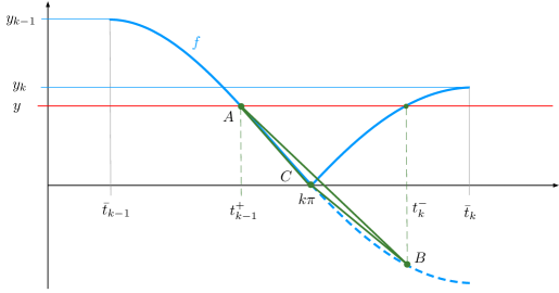
Figure 2. The slope of the segment $AB$ is not smaller than the slope of either $AC$ or $BC$.

$$\frac{2y}{t_{k}^{-}-t_{k-1}^{+}}=\frac{\left|\frac{\sin t_{k}^{-}}{t_{k}^{-}}-\frac{\sin t_{k-1}^{+}}{t_{k-1}^{+}}\right|}{t_{k}^{-}-t_{k-1}^{+}} =|\text{slope}(AB)|$$

$$\geqslant\min\left\{|\text{slope}(AC)|,|\text{slope}(BC)|\right\}.$$

Let $\bar{t}_{k}\in(k\pi,(k+1)\pi)$ denote the point where $f(t)$ attains its local maximum $y_{k}$ on $(k\pi,(k+1)\pi)$. Observe that

$$|\text{slope}(BC)|=\frac{|\sin t_{k}^{-}|}{t_{k}^{-}(t_{k}^{-}-k\pi)}\geqslant\frac{y_{k}}{\bar{t}_{k}-k\pi}\geqslant\frac{y_{k}}{\pi},$$

where the first inequality follows from Lemma 12 (i) applied to $t_{k}^{-}<\bar{t}_{k}$. Similarly,

$$|\text{slope}(AC)|=\frac{|\sin t_{k-1}^{+}|}{t_{k-1}^{+}(k\pi-t_{k-1}^{+})}\geqslant\min\left\{\frac{y_{k-1}}{k\pi-\bar{t}_{k-1}},\frac{1}{k\pi}\right\}\geqslant\min\left\{\frac{y_{k-1}}{\pi},\frac{1}{k\pi}\right\},$$

where in the first inequality we use Lemma 12 (ii) to lower bound the function in question by the minimum of its values at the end-points $t=\bar{t}_{k-1}$ and $t=k\pi$. Finally, putting these two estimates together and using $y_{k}>\frac{1}{\pi(k+\frac{1}{2})}$, we obtain

$$|\text{slope}(AB)|\geqslant\frac{1}{\pi^{2}(k+\frac{1}{2})}$$

and, consequently,

$$t_{k}^{-}-t_{k-1}^{+}{=\frac{2y}{|\text{slope}(AB)|}}\leqslant 2\pi^{2}y\left(k+\frac{1}{2}\right),$$

which results in

$$F(y)<2\pi^{-p+1}y\left(\frac{3}{2}0.98^{-p-1}+\frac{5}{2}1.97^{-p-1}+\sum_{k=3}^{m}\left(k+\frac{1}{2}\right)(k-1)^{-p-1}\right)+\frac{1}{p}(m\pi)^{-p}.$$

Since $y>y_{m+1}>\frac{1}{(m+\frac{3}{2})\pi}$, and $m\geqslant 30$, we have

$$\frac{1}{p}(m\pi)^{-p}<\frac{1}{p}\left(\frac{m+3/2}{m}\right)^{p}y^{p}\leqslant\frac{1}{p}1.05^{p}y^{p}.$$

Moreover, since $y<y_{m}<\frac{1}{m\pi}$, we have (crudely), $m-1<\frac{1}{\pi y}$ and bounding the sum using the integral, we obtain

$$\sum_{k=3}^{m}\left(k+\frac{1}{2}\right)(k-1)^{-p-1} =\sum_{k=2}^{m-1}\frac{k+\frac{3}{2}}{k^{p+1}}$$

$$<\int_{1}^{m-1}\left(x^{-p}+\frac{3}{2}x^{-p-1}\right)\mathrm{d}x$$

$$<\frac{(\pi y)^{p-1}-1}{1-p}+\frac{3(1-(\pi y)^{p})}{2p}.$$

Therefore, in order to have $F(y)<G(y)$, it suffices to guarantee that

$$2\pi^{-p+1}y\Bigg{(}\frac{3}{2}0.98^{-p-1}+\frac{5}{2}1.97^{-p-1} +\frac{(\pi y)^{p-1}-1}{1-p}+\frac{3(1-(\pi y)^{p})}{2p}\Bigg{)}$$

$$\qquad+\frac{1}{p}1.05^{p}y^{p}<\frac{1}{p}\left(-6\log y\right)^{-p/2}$$

holds for every $0<p<1$ and $0<y<\frac{1}{30\pi}$. Since $-y\log y$ is increasing for $y<\frac{1}{e}$, we have $-\log y<\frac{\log(30\pi)}{30\pi}\frac{1}{y}$ for $0<y<\frac{1}{30\pi}$. By monotonicity, for $0<p<1$, we have $\frac{3}{2}0.98^{-p-1}+\frac{5}{2}1.97^{-p-1}<\frac{3}{2}0.98^{-1-1}+\frac{5}{2}1.97^{-1}<3$. It remains to use Lemma 14. This shows that Condition (ii) holds and the proof of the lemma is complete. It remains to show Claims A and B. ∎

Proof of Claim A.

By the integral representation for the $p$-norm from Lemma 4,

$$\kappa_{p}H(p,2)=\mathbb{E}|U_{1}+U_{2}|^{p}-\mathbb{E}\left|\sqrt{\frac{2}{3}}Z\right|^{p}=\frac{2^{p+1}}{(p+1)(p+2)}-\frac{1}{\sqrt{\pi}}\left(\frac{4}{3}\right)^{p/2}\Gamma\left(\frac{1+p}{2}\right).$$

By Lemma 16, it suffices to prove that $2^{p+1}>(p+2)\left(1+\frac{p(p+1)}{6}\right)$ for all $0<p<1$. The 3rd derivative of the difference changes sign once on $(0,1)$ from $-$ to $+$. The 2nd derivative is negative at the end-points $p=0$ and $p=1$, so it is negative on $(0,1)$ and hence the difference is concave. It vanishes at the end-points $p=0$ and $p=1$, which finishes the argument. ∎

Proof of Claim B.

Our argument is split into two steps: first we show that $H(p,1)$ increases with $p$ and then we estimate $H(0.6,1)$. For somewhat similar computations, but related to random signs, see Section 5 in [21]. In Step 1, to numerically evaluate the integrals in question, we will frequently use that given $0<a<b$ and an integer $m$, integrals of the form $\int_{a}^{b}(\sin t)t^{-m}\mathrm{d}t$ can be efficiently estimated to an arbitrary precision by expressing them in terms of the trigonometric integral functions $\text{Si},\text{Ci}$. The same applies to the integrals of the form $\int_{a}^{b}e^{-t^{2}}t^{q}\mathrm{d}t$ with $0<a<b\leqslant\infty$ and real $q$, thanks to reductions to the incomplete gamma function $\Gamma$ and the exponential integral Ei. We recall that for $x>0$, $s\neq 0,-1,-2,\dots$,

$$\text{Si}(x) =-\int_{x}^{\infty}\frac{\sin t}{t}\mathrm{d}t=-\frac{\pi}{2}-\sum_{k=1}^{\infty}\frac{(-1)^{k}x^{2k-1}}{(2k-1)(2k-1)!},$$

$$\text{Ci}(x) =-\int_{x}^{\infty}\frac{\cos t}{t}\mathrm{d}t=\gamma+\log x+\sum_{k=1}^{\infty}(-1)^{k}\frac{x^{2k}}{2k(2k)!},$$

$$\text{Ei}(-x) =-\int_{x}^{\infty}\frac{e^{-t}}{t}\mathrm{d}t=\gamma+\log x+\sum_{k=1}^{\infty}\frac{(-x)^{k}}{k\cdot k!},$$

$$\Gamma(s,x) =\int_{x}^{\infty}t^{s-1}e^{-t}\mathrm{d}t=\Gamma(s)-\sum_{k=0}^{\infty}\frac{(-1)^{k}x^{s+k}}{k!(s+k)}$$

(here $\gamma=0.57721..$ is the Euler-Mascheroni constant). These series representations allow to obtain arbitrarily good numerical approximations to these integrals.

In Step 2, all the numerical computations are reduced to integrals of the form $\int_{a}^{b}\frac{\mathrm{d}t}{t^{q}}$ which are explicit.

Step 1: $\frac{\partial}{\partial p}H(p,1)>0$, $0.6<p<1$. We have,

$$\frac{\partial}{\partial p}H(p,1)=\int_{0}^{\infty}(-\log t)\frac{g(t)-f(t)}{t^{p+1}}\mathrm{d}t.$$

We break the integral into several regions. Recall $g>f$ on $(0,\pi)$, by Lemma 7. Thus, plainly,

$$\int_{0}^{1}(-\log t)\frac{g(t)-f(t)}{t^{p+1}}\mathrm{d}t>0.$$

Moreover, $g-f$ changes sign from $+$ to $-$ exactly once on $(\pi,4)$ at $t=3.578..$. Let $t_{0}=3.57$. On $(1,t_{0})$, using $t^{-p-1}=t^{1-p}t^{-2}\leqslant t_{0}^{1-p}t^{-2}$, we obtain

$$\int_{1}^{t_{0}}(-\log t)\frac{g(t)-f(t)}{t^{p+1}}\mathrm{d}t\geqslant t_{0}^{1-p}\int_{1}^{t_{0}}(-\log t)\frac{g(t)-f(t)}{t^{2}}\mathrm{d}t>-0.0297\cdot t_{0}^{1-p},$$

where in the last inequality we use $\log t\leqslant\log\frac{5}{2}+\frac{2}{5}(t-\frac{5}{2})$ (by concavity) and then estimate the resulting integrals. Now,

$$\int_{t_{0}}^{\infty}(-\log t)\frac{g(t)-f(t)}{t^{p+1}}\mathrm{d}t=\int_{t_{0}}^{\infty}(\log t)\frac{f(t)}{t^{p+1}}\mathrm{d}t-\int_{t_{0}}^{\infty}(\log t)\frac{g(t)}{t^{p+1}}\mathrm{d}t.$$

For $t>t_{0}$, $t^{-p-1}=t^{1-p}t^{-2}>t_{0}^{1-p}t^{-2}$ and for $k\geqslant 1$, $\log t\geqslant\ell_{k}(t)$ on $(k\pi,(k+1)\pi)$ with

$$\ell_{k}(t)=\frac{(k+1)\pi-t}{\pi}\log(k\pi)+\frac{t-k\pi}{\pi}\log((k+1)\pi),$$

thus

$$\int_{t_{0}}^{\infty}(\log t)\frac{f(t)}{t^{p+1}}\mathrm{d}t \geqslant t_{0}^{1-p}\left(\int_{t_{0}}^{2\pi}\ell_{1}(t)\frac{-\sin t}{t^{3}}\mathrm{d}t+\sum_{k=2}^{n}\int_{k\pi}^{(k+1)\pi}\ell_{k}(t)\frac{(-1)^{k}\sin t}{t^{3}}\mathrm{d}t\right).$$

For $n=5$, this gives

$$\int_{t_{0}}^{\infty}(\log t)\frac{f(t)}{t^{p+1}}\mathrm{d}t>0.0437\cdot t_{0}^{1-p}.$$

Finally, since $\log u\leqslant\frac{u}{e}$, $u>0$, we have $\frac{\log t}{t^{p}}<\frac{1}{ep}<\frac{1}{0.6e}<0.6132<0.6132\cdot t_{0}^{1-p}$, thus

$$\int_{t_{0}}^{\infty}(\log t)\frac{g(t)}{t^{p+1}}\mathrm{d}t\leqslant 0.6132\cdot t_{0}^{1-p}\int_{t_{0}}^{\infty}\frac{e^{-t^{2}/6}}{t}\mathrm{d}t<0.0127\cdot t_{0}^{1-p}.$$

Putting these together yields

$$\frac{\partial}{\partial p}H(p,1)>(0.0437-0.0297-0.0127)t_{0}^{1-p}=0.0013\cdot t_{0}^{1-p}>0.$$

Step 2: $H(0.6,1)>0$. We have,

$$H(0.6,1)=\int_{0}^{\pi}\frac{e^{-t^{2}/6}-\frac{\sin t}{t}}{t^{8/5}}\mathrm{d}t+\int_{\pi}^{\infty}\frac{e^{-t^{2}/6}}{t^{8/5}}\mathrm{d}t-\int_{\pi}^{\infty}\frac{|\sin t|}{t^{13/5}}\mathrm{d}t.$$

On $(0,\pi)$, we use Taylor’s polynomials to bound the integrand,

$$e^{-t^{2}/6}-\frac{\sin t}{t}>\sum_{k=0}^{7}\frac{(-t^{2}/6)^{k}}{k!}-\sum_{k=0}^{6}\frac{(-1)^{k}t^{2k}}{(2k+1)!}.$$

Plugging this into the integral results in

$$\int_{0}^{\pi}\frac{e^{-t^{2}/6}-\frac{\sin t}{t}}{t^{8/5}}\mathrm{d}t>0.0434.$$

Using the incomplete Gamma function,

$$\int_{\pi}^{\infty}\frac{e^{-t^{2}/6}}{t^{8/5}}\mathrm{d}t>0.0184.$$

Finally,

$$\int_{\pi}^{\infty}\frac{|\sin t|}{t^{13/5}}\mathrm{d}t =\int_{0}^{\pi}(\sin t)\left(\sum_{k=1}^{\infty}\frac{1}{(t+k\pi)^{13/5}}\right)\mathrm{d}t$$

$$\leqslant\int_{0}^{\pi}(\sin t)\left(\sum_{k=1}^{n}\frac{1}{(t+k\pi)^{13/5}}\right)\mathrm{d}t+\int_{(n+1)\pi}^{\infty}\frac{\mathrm{d}t}{t^{13/5}}.$$

We use Taylor’s polynomial again, $\sin t\leqslant 1-\frac{1}{2}(t-\pi/2)^{2}+\frac{1}{24}(t-\pi/2)^{4}$. Choosing $n=8$ gives

$$\int_{\pi}^{\infty}\frac{|\sin t|}{t^{13/5}}\mathrm{d}t<0.0615.$$

Adding up these estimates yields $H(0.6,1)>0.0434+0.0184-0.0615=0.0003$. ∎

5. Inductive argument

As explained in Section 2, Theorem 6 gives the following corollary (we use homogeneity to rewrite (4) in an equivalent form, better suited for the ensuing arguments). Recall $c_{p}=\|Z\|_{p}/\sqrt{3}$ and define

$$\varphi_{p}(x)=(1+x)^{p/2},\qquad x\geqslant 0.$$

Corollary 19.

Let $0<p<1$. For every $n\geqslant 2$ and real numbers $a_{2},\dots,a_{n}$ with $\sum_{j=2}^{n}a_{j}^{2}\geqslant 1$ and $a_{j}^{2}\leqslant 1$ for every $j=2,\ldots,n$, we have

$$\mathbb{E}\left|U_{1}+\sum_{j=2}^{n}a_{j}U_{j}\right|^{p}\geqslant c_{p}^{p}\cdot\varphi_{p}\left(\sum_{j=2}^{n}a_{j}^{2}\right).$$

The goal here is to remove the restriction on the $a_{j}$’s. The key idea from [24] is to replace $\varphi_{p}$ with a pointwise larger function, thereby strengthening the inequality and to proceed by induction on $n$. We use the function from [24],

$$\Phi_{p}(x)=\begin{cases}\varphi_{p}(x),&x\geqslant 1,\\ 2\varphi_{p}(1)-\varphi_{p}(2-x),&0\leqslant x\leqslant 1.\end{cases}$$

Even though this function changes from being convex to concave at $x=1$, it is designed to satisfy the following extended convexity property on $[0,2]$, crucial for the proof.

Lemma 20 (Nazarov-Podkorytov, [24]).

For every $0<p<2$ and $a,b\in[0,2]$ with $a+b\leqslant 2$, we have

$$\frac{\Phi_{p}(a)+\Phi_{p}(b)}{2}\geqslant\Phi_{p}\left(\frac{a+b}{2}\right).$$

As in [4], in order to have certain algebraic identities, we run the argument for $\xi_{1},\xi_{2},\dots$, independent random vectors in $\mathbb{R}^{3}$ uniformly distributed on the centred unit Euclidean sphere $S^{2}$. Here $\left\langle\cdot,\cdot\right\rangle$ and $\|\cdot\|$ is the standard inner product and the resulting Euclidean norm in $\mathbb{R}^{3}$, respectively.

Theorem 21.

Let $0<p<0.69$. For every $n\geqslant 2$ and vectors $v_{2},\dots,v_{n}$ in $\mathbb{R}^{3}$, we have

(10) $$\mathbb{E}\left|\left\langle e_{1},\xi_{1}\right\rangle+\sum_{j=2}^{n}\left\langle v_{j},\xi_{j}\right\rangle\right|^{p}\geqslant c_{p}^{p}\cdot\Phi_{p}\left(\sum_{j=2}^{n}\|v_{j}\|^{2}\right).$$

Here $e_{1}=(1,0,0)$, the unit vector of the standard basis.

Note $\left\langle v_{j},\xi_{j}\right\rangle$ has the same distribution as $\|v_{j}\|U_{j}$ (by rotational invariance, $\left\langle v_{j},\xi_{j}\right\rangle$ has the same distribution as $\|v_{j}\|\left\langle e_{1},\xi_{j}\right\rangle$ and by the Archimedes’ hat-box theorem, the projection $\left\langle e_{1},\xi_{j}\right\rangle$ is a uniform random variable on $[-1,1]$). Since $\Phi_{p}\geqslant\varphi_{p}$, this gives Theorem 1 for $0<p<0.69$, thereby completing its proof. It remains to show Theorem 21, which is done by repeating almost verbatim the proof of Theorem 18 from [4]. We repeat the argument for the convenience of the reader. To adjust the proof of the base case we will need the following lemma.

Lemma 22.

For every $0<x<1$ and $0<p<0.69$, we have

$$\frac{(1+x)^{2+p}-(1-x)^{2+p}}{2(2+p)x} >\frac{1+p}{\sqrt{\pi}}\Gamma\left(\frac{1+p}{2}\right)\left(\frac{2}{3}\right)^{p/2}\left(2^{1+p/2}-(3-x^{2})^{p/2}\right)$$

$${=(\|Z\|_{p}/\sqrt{3})^{p}(1+p)\Phi_{p}(x^{2}).}$$

Proof.

We first observe that keeping only the first two terms in the binomial series expansion, we obtain

$$\frac{(1+x)^{2+p}-(1-x)^{2+p}}{2(2+p)x}=\sum_{k=0}^{\infty}\frac{1}{p+2}\binom{p+2}{2k+1}x^{2k}>1+\frac{p(p+1)}{6}x^{2},$$

because all the terms are positive. It thus suffices to show that for every $0<x<1$ and $0<p<0.69$,

$$1+\frac{p(p+1)}{6}x+\frac{1+p}{\sqrt{\pi}}\Gamma\left(\frac{1+p}{2}\right)\left(\frac{2}{3}\right)^{p/2}\left((3-x)^{p/2}-2^{1+p/2}\right)>0$$

(we have replaced $x^{2}$ by $x$). By the evident concavity in $x$, it suffices to check that the inequality holds at the end-points $x=0$ and $x=1$ which follows from Lemmas 16 and 15, respectively. ∎

Proof of Theorem 21.

For the case $n=2$, we need to show that for every $v\in\mathbb{R}^{3}$

(11) $$\mathbb{E}|\langle e_{1},\xi_{1}\rangle+\langle v,\xi_{2}\rangle|^{p}\geqslant c_{p}^{p}\Phi_{p}(\|v\|^{2}).$$

We first reduce this claim to the case $\|v\|\leqslant 1$: If $\|v\|>1$ then due to rotational invariance

$$\mathbb{E}|\langle e_{1},\xi_{1}\rangle+\langle v,\xi_{2}\rangle|^{p} =\|v\|^{p}\mathbb{E}\left|\langle\frac{e_{1}}{\|v\|},\xi_{1}\rangle+\langle\frac{v}{\|v\|},\xi_{2}\rangle\right|^{p}$$

$$=\|v\|^{p}\mathbb{E}|\langle v^{\prime},\xi_{1}\rangle+\langle e_{1},\xi_{2}\rangle|^{p},$$

where $v^{\prime}\in\mathbb{R}^{3}$ is such that $\|v^{\prime}\|=\frac{1}{\|v\|}<1$. On the other hand, due to homogeneity,

$$\Phi_{p}(\|v\|^{2})=\phi_{p}(\|v\|^{2})=\|v\|^{p}\phi_{p}(\|v^{\prime}\|^{2}),$$

so (11) is equivalent to

$$\mathbb{E}|\langle v^{\prime},\xi_{1}\rangle+\langle e_{1},\xi_{2}\rangle|^{p}\geqslant c_{p}^{p}\phi_{p}(\|v^{\prime}\|^{2}),\qquad\|v^{\prime}\|\leqslant 1$$

and since $\Phi_{p}(x)\geqslant\phi_{p}(x)$ for $x\in[0,1]$ it is indeed sufficient to restrict to the case $\|v\|\leqslant 1$.

In this case, we set $x:=\|v\|\leqslant 1$ and compute explicitly the left and right hand side of (11) to deduce that

$$\mathbb{E}|\langle e_{1},\xi_{1}\rangle+\langle v,\xi_{2}\rangle|^{p} =\mathbb{E}|U_{1}+xU_{2}|^{p}=\frac{(1+x)^{2+p}-(1-x)^{2+p}}{2(1+p)(2+p)x}\geqslant c_{p}^{p}\Phi_{p}(x^{2})$$

with the aid of Lemma 22.

For the inductive step, let $n\in\mathbb{N}$ and assume that (10) holds for every $v_{2},\ldots,v_{n-1}\in\mathbb{R}^{3}$. We let $v_{2},\ldots,v_{n}\in\mathbb{R}^{3}$, $x:=\sum_{k=2}^{n}\|v\|^{2}$ and distinguish between the following mutually exclusive cases.

Case (i): $\|v_{k}\|>1$ for some $2\leqslant k\leqslant n$. Then $x>1$ and the wanted inequality is

$$\mathbb{E}\left|\sum_{k=1}^{n}\langle v_{k},\xi_{k}\rangle\right|^{p}\geqslant c_{p}^{p}\left(\sum_{k=1}^{n}\|v_{k}\|^{2}\right)^{p/2}$$

with $v_{1}=e_{1}$. For $k=1,\ldots,n$ we let $v_{k}^{\prime}=\frac{v_{k}^{\ast}}{\|v_{1}^{\ast}\|}$, where $v_{1}^{*},\ldots,v_{n}^{*}$ is any rearrangement of $v_{1},\ldots,v_{n}$ with $\|v_{k}^{\ast}\|\geqslant\|v_{k+1}^{\ast}\|$ for every $k=1,\ldots,n-1$. Then $\|v^{\prime}_{1}\|=1$ and $\|v_{k}^{\prime}\|\leqslant 1$ for $k=2,\ldots,n$. Due to homogeneity and the fact that $\langle v_{1}^{\prime},\xi_{1}\rangle$ has the same distribution as $\langle e_{1},\xi_{1}\rangle$ it is enough to prove

$$\mathbb{E}\left|\langle e_{1},\xi_{1}\rangle+\sum_{k=2}^{n}\langle v_{k}^{\prime},\xi_{k}\rangle\right|^{p}\geqslant c_{p}^{p}\Phi_{p}\left(\sum_{k=2}^{n}\|v_{k}^{\prime}\|^{2}\right).$$

This is done on the next cases.

Case (ii): $\|v_{k}\|\leqslant 1$ for every $2\leqslant k\leqslant n$ and $x\geqslant 1$. We then again have that $\Phi_{p}(x)=\phi_{p}(x)$, and the desired inequality (10) coincides with

$$\mathbb{E}\left|\sum_{k=1}^{n}\langle v_{k},\xi_{k}\rangle\right|^{p}\geqslant c_{p}^{p}\left(\sum_{k=1}^{n}\|v_{k}\|^{2}\right)^{p/2}.$$

Note that here we have

$$\max_{1\leqslant k\leqslant n}\|v_{k}\|=1\leqslant\frac{1}{2}\left(1+x\right)=\frac{1}{2}\sum_{k=1}^{n}\|v_{k}\|^{2},$$

and since the distribution of $\sum_{k=1}^{n}\langle v_{k},\xi_{k}\rangle$ is identical to that of $\sum_{k=1}^{n}\|v_{k}\|U_{k}$ it is clear that this case is handled by Theorem 6.

Case (iii): $\|v_{k}\|\leqslant 1$ for every $2\leqslant k\leqslant n$ and $x<1$. We use the fact that $(\xi_{n-1},\xi_{n})$ has the same distribution as $(\xi_{n-1},Q\xi_{n-1})$ where $Q$ is a random orthogonal matrix independent of all the $\xi_{k}$’s to write

$$\mathbb{E}\left|\langle e_{1},\xi_{1}\rangle+\sum_{k=2}^{n}\langle v_{k},\xi_{k}\rangle\right|^{p}=\mathbb{E}|\langle e_{1},\xi_{1}\rangle+\langle v_{2},\xi_{2}\rangle+\ldots+\langle v_{n-1},\xi_{n-1}\rangle+\langle Q^{\top}v_{n},\xi_{n-1}\rangle|^{p}$$

$$\hskip 55.0pt=\mathbb{E}_{Q}\left[\mathbb{E}_{(\xi_{k})_{k=2}^{n-1}}|\langle e_{1},\xi_{1}\rangle+\langle v_{2},\xi_{2}\rangle+\ldots+\langle v_{n-2},\xi_{n-2}\rangle+\langle Q^{\top}v_{n},\xi_{n-1}\rangle|^{p}\right].$$

By the inductive hypothesis applied to $(v_{2},\ldots,v_{n-2},v_{n-1}+Q^{\top}v_{n})$ (conditioned on the value of $Q$) we get

$$\mathbb{E}\left|\langle e_{1},\xi_{1}\rangle+\sum_{k=2}^{n}\langle v_{k},\xi_{k}\rangle\right|^{p}\geqslant c_{p}^{p}\mathbb{E}_{Q}\Phi_{p}(\|v_{2}\|^{2}+\ldots+\|v_{n-2}\|^{2}+\|v_{n-1}+Q^{\top}v_{n}\|^{2}).$$

Finally note that

$$\mathbb{E}_{Q}\Phi_{p}\left(\sum_{k=2}^{n-2}\|v_{k}\|^{2}+\|v_{n-1}+Q^{\top}v_{n}\|^{2}\right)=$$

$$\hskip 55.0pt=\mathbb{E}_{Q}\frac{\Phi_{p}(x+2\langle v_{n-1}+Q^{\top}v_{n}\rangle)+\Phi_{p}(x-2\langle v_{n-1}+Q^{\top}v_{n}\rangle)}{2}\geqslant\Phi_{p}(x)$$

by the symmetry of $\Phi_{p}$ and Lemma 20 (applied for $a=x+2\langle v_{n-1}+Q^{\top}v_{n}\rangle$ and $b=x-2\langle v_{n-1}+Q^{\top}v_{n}\rangle$ which satisfy $a+b=2x\leqslant 2$). This concludes the proof of the inductive step. ∎

6. Rényi entropy: Proof of Theorem 2

For the lower bound,

$$h_{p}\left(\sum_{j}a_{j}U_{j}\right)\geqslant h_{1}\left(\sum_{j}a_{j}U_{j}\right)\geqslant h_{1}(U_{1}),$$

where the first inequality follows from the fact that $p\mapsto h_{p}(\cdot)$ is nonincreasing and the second one is justified by the entropy power inequality (see, e.g. Theorem 4 in [6]). It remains to notice that $h_{p}(U_{1})=\log 2$ for every $p$.

Towards the upper bound, we first note that for nonnegative functions $f$ and $g$, $0<p<1$, we have

$$\left(\int f^{p}\right)^{\frac{1}{p}}\left(\int g^{p}\right)^{\frac{p-1}{p}}\leqslant\int fg^{p-1}.$$

This follows directly from Hölder’s inequality. Now, fix a unit vector $a$ in $\mathbb{R}^{n}$, let $f$ be the density of $\sum_{j}a_{j}U_{j}$ and $g(x)=(2\pi/3)^{-1/2}e^{-x^{2}/6}$, the density of $Z/\sqrt{3}$. In view of the above inequality, it suffices to show that

$$\int fg^{p-1}\leqslant\int gg^{p-1}.$$

Since

$$g(x)^{p-1}=(2\pi/3)^{\frac{1-p}{2}}\sum_{k=0}^{\infty}\frac{1}{k!}\left(\frac{1-p}{6}\right)^{k}x^{2k},$$

it suffices to show that for each positive integer $k$,

$$\mathbb{E}\left(\sum a_{j}U_{j}\right)^{2k}=\int x^{2k}f(x)\mathrm{d}x\leqslant\int x^{2k}g(x)\mathrm{d}x=\mathbb{E}\left(\frac{Z}{\sqrt{3}}\right)^{2k}.$$

This follows from the main result of [19], that $C_{p}=\|Z\|_{p}/\sqrt{3}$, $p>1$, see (2). $\square$

We finish by remarking that the problem of maximising $h_{p}(\sum a_{j}U_{j})$ under a variance constraint for a fixed number of summands to the best of our knowledge remains wide open for $p\in(0,\infty)$. The case of Shannon entropy, $p=1$, seems to be the most important and interesting, see Question 9 in [7], or Question 3 in [3], also comprehensively presenting many other related and tangential problems. The natural conjecture is that: $h_{1}(\sum_{j=1}^{n}a_{j}U_{j})\leqslant h_{1}(\sum_{j=1}^{n}\frac{1}{\sqrt{n}}U_{j})$, for every unit vector $a$ in $\mathbb{R}^{n}$ (see 8.3.1 in [3] for a conceivable approach). The case $p=0$ is of course trivial, whereas the case $p=\infty$ amounts to the cube-slicing inequalities: $h_{\infty}(\sum_{j=1}^{n}a_{j}U_{j})\leqslant h_{\infty}(U_{1})$ is due to Hadwiger and, independently, Hensley (see [10, 12]), $h_{\infty}(\sum_{j=1}^{n}a_{j}U_{j})\geqslant h_{\infty}((U_{1}+U_{2})/\sqrt{2})$ is due to Ball (see [2]).

References

- [1] Baernstein, A., II, Culverhouse, R., Majorization of sequences, sharp vector Khinchin inequalities, and bisubharmonic functions. Studia Math. 152 (2002), no. 3, 231–248.
- [2] Ball, K., Cube slicing in . Proc. Amer. Math. Soc. 97 (1986), no. 3, 465–473.
- [3] Bartczak, M., Nayar, P., Zwara, S., Sharp variance-entropy comparison for nonnegative Gaussian quadratic forms, preprint (2020), arXiv:2005.11705.
- [4] Chasapis, G. König, H., Tkocz, T., From Ball’s cube slicing inequality to Khinchin-type inequalities for negative moments, preprint (2020), arXiv:2011.12251.
- [5] Costa, J., Hero, A., Vignat, C., On solutions to multivariate maximum -entropy problems, Lecture Notes in Computer Science, vol. 2683, Springer-Verlag, Berlin, 2003, pp. 211–228.
- [6] Dembo, A., Cover, T. M., Thomas, J. A., Information-theoretic inequalities. IEEE Trans. Inform. Theory 37 (1991), no. 6, 1501–1518.
- [7] Eskenazis, A., Nayar, P., Tkocz, T., Gaussian mixtures: entropy and geometric inequalities, Ann. of Prob. 46(5) 2018, 2908–2945.
- [8] Eskenazis, A., Nayar, P., Tkocz, T., Sharp comparison of moments and the log-concave moment problem. Adv. Math. 334 (2018), 389–416.
- [9] Haagerup, U., The best constants in the Khintchine inequality. Studia Math. 70 (1981), no. 3, 231–283.
- [10] Hadwiger, H. Gitterperiodische Punktmengen und Isoperimetrie. Monatsh. Math. 76 (1972), 410–418.
- [11] Havrilla, A., Nayar, P., Tkocz, T., Khinchin-type inequalities via Hadamard’s factorisation, preprint (2021), arXiv:2102.09500.
- [12] Hensley, D., Slicing the cube in and probability (bounds for the measure of a central cube slice in by probability methods). Proc. Amer. Math. Soc. 73 (1979), no. 1, 95–100.
- [13] Johnson, O., Vignat, C., Some results concerning maximum Rényi entropy distributions. Ann. Inst. H. Poincaré Probab. Statist. 43 (2007), no. 3, 339–351.
- [14] Khintchine, A., Über dyadische Brüche. Math. Z. 18 (1923), no. 1, 109–116.
- [15] König, H., On the best constants in the Khintchine inequality for Steinhaus variables. Israel J. Math. 203 (2014), no. 1, 23–57.
- [16] König, H., Kwapień, S., Best Khintchine type inequalities for sums of independent, rotationally invariant random vectors. Positivity 5 (2001), no. 2, 115–152.
- [17] Kwapień, S., Latała, R., Oleszkiewicz, K., Comparison of moments of sums of independent random variables and differential inequalities. J. Funct. Anal. 136 (1996), no. 1, 258–268.
- [18] Latała, R., Oleszkiewicz, K., On the best constant in the Khinchin-Kahane inequality. Studia Math. 109 (1994), no. 1, 101–104.
- [19] Latała, R., Oleszkiewicz, K., A note on sums of independent uniformly distributed random variables. Colloq. Math. 68 (1995), no. 2, 197–206.
- [20] Lutwak, E,. Yang, D., Zhang, G., Cramér-Rao and moment-entropy inequalities for Rényi entropy and generalized Fisher information. IEEE Trans. Inform. Theory 51 (2005), no. 2, 473–478.
- [21] Mordhorst, O., The optimal constants in Khintchine’s inequality for the case . Colloq. Math. 147 (2017), no. 2, 203–216.
- [22] Moriguti, S., A lower bound for a probability moment of any absolutely continuous distribution with finite variance. Ann. Math. Statistics 23 (1952), 286–289.
- [23] Nayar, P., Oleszkiewicz, K., Khinchine type inequalities with optimal constants via ultra log-concavity. Positivity 16 (2012), no. 2, 359–371.
- [24] Nazarov, F., Podkorytov, A., Ball, Haagerup, and distribution functions. Complex analysis, operators, and related topics, 247–267, Oper. Theory Adv. Appl., 113, Birkhäuser, Basel, 2000.
- [25] Rényi, A., On measures of entropy and information. 1961 Proc. 4th Berkeley Sympos. Math. Statist. and Prob., Vol. I pp. 547–561 Univ. California Press, Berkeley, Calif.
- [26] Szarek, S., On the best constant in the Khintchine inequality. Stud. Math. 58, 197– 208 (1976).