Symmetry-driven graph neural networks

Abstract

Exploiting symmetries and invariance in data is a powerful, yet not fully exploited, way to achieve better generalisation with more efficiency. In this paper, we introduce two graph network architectures that are equivariant to several types of transformations affecting the node coordinates. First, we build equivariance to any transformation in the coordinate embeddings that preserves the distance between neighbouring nodes, allowing for equivariance to the Euclidean group. Then, we introduce angle attributes to build equivariance to any angle preserving transformation - thus, to the conformal group. Thanks to their equivariance properties, the proposed models can be vastly more data efficient with respect to classical graph architectures, intrinsically equipped with a better inductive bias and better at generalising. We demonstrate these capabilities on a synthetic dataset composed of $n$-dimensional geometric objects. Additionally, we provide examples of their limitations when (the right) symmetries are not present in the data.

1 Introduction

Symmetries exist throughout nature. All the fundamental laws of physics are built upon the framework of symmetries, from the gauge groups describing the Standard Model of particle physics, to Einstein’s theories of general and special relativity. Once one understands the symmetry of a certain system, powerful predictions can be made. A notable example is that of Gell-Mann’s eightfold-way (Gell-Mann, 1961), built upon the symmetries observed in hadrons, that led to his prediction of the $\Omega^{-}$ baryon, which was subsequently observed 3 years later (Barnes et al., 1964). The study of symmetries and invariance in deep learning has recently become a field of interest to the community (see, e.g., (Bronstein et al., 2021) for a comprehensive overview), and rapid progress has been made in constructing architectures with group theoretic structures embedded within. Two fundamental architectures in machine learning, the convolutional and graph neural networks, are invariant to the translation and symmetry groups respectively.

Graph networks in particular are designed to learn from graph-structured data and are by construction permutation equivariant with respect to the input. They were originally proposed in (Gori et al., 2005; Scarselli et al., 2008) and have received a lot of attention in the last years (see, e.g., (Battaglia et al., 2018; Hamilton, 2020; Wu et al., 2020) for a comprehensive overview). Due to their properties, they find application in a broad range of problems like learning the dynamics of complex physical systems (Sanchez-Gonzalez et al., 2020; Pfaff et al., 2021), particle identification in particle physics (Dreyer and Qu, 2021), learning causal and relational graphs (Kipf et al., 2018; Li et al., 2020), discovering symbolic models (Cranmer et al., 2020), as well as quantum chemistry (Gilmer et al., 2017) and drug discovery (Stokes et al., 2020).

In this work, we start from standard graph neural networks and extend them to build, in addition to permutation equivariance, equivariance to many transformations affecting the node coordinates, possibly belonging to important groups. First, we define the distance preserving graph network (DGN) which, thanks to modified update rules, is equivariant to any transformation in the coordinate embeddings that preserves the distance between neighbouring nodes. An example of such a transformation is the Hoberman sphere, whose 3D shape changes while preserving distances between connected nodes. As an important particular case, we show that the architecture is equivariant to the $n$-dimensional Euclidean group. An additional input layer can also make it equivariant to dilations in the coordinates via the conformal orthogonal group. Then, we define the angle preserving graph network (AGN), which is equivariant to any transformation preserving the angles between triples of neighbouring nodes in the graph (molecular conformations are a notable example of such transformations) and, thus, to the $n$-dimensional conformal group on $\mathbb{R}^{n}$.

By constructing such architectures, we enable a wide range of possible transformations to be performed on graph-structured data, with the only requirement being that distances or angles between coordinates of neighbouring nodes are preserved. This means that both networks are equivariant to translations, rotations, reflections (i.e., the Euclidean group, $E(n)$), with the AGN being also equivariant to dilations, inversions and non-orthogonal rotations. In practice, this means the networks are able to filter out many copies of the same input whose coordinate embeddings have been simply rotated, moved or scaled and therefore learn more efficiently than architectures which consider the inputs as distinct. In other words, a single sample contains the same information as many copies of it obtained by appropriately transforming it. Finally, while the two architectures we present are partially overlapping in terms of equivariance features, it is important to consider specific use cases where the use of one architecture over another would be preferred.

Thanks to their properties, the proposed models are able to learn much more efficiently and generalise better than standard graph networks, even when data are transformed in highly non-trivial ways. We demonstrate this on a synthetic dataset consisting of $n$-dimensional geometric shapes and other benchmark datasets. Moreover, we show examples of cases in which using our architectures is counterproductive due to the lack of symmetries in the data.

2 Background

2.1 Group theory and equivariance

Group theory provides the mathematical formulation for symmetries of systems, with symmetry operations represented by individual group elements. A group can be defined as a set $G$ equipped with a binary operation, which enables one to combine two group elements to form a third, whilst preserving the group axioms (associativity, identity, closure and inverse). A function unaffected by a group action is said to be invariant, which is particular instance of equivariance. Formally, let $X\subseteq\mathbb{R}^{n}$ and $\varphi_{g}:X\to X$ be a transformation on $X$ for a group element $g\in G$. Then, the linear map $\Phi:X\to Y$, $Y\subseteq\mathbb{R}^{n}$, is equivariant to $G$ if $\forall g\in G$, $\exists\varphi_{g}^{\prime}:Y\to Y$ such that

$$\Phi(\varphi_{g}(\mathbf{x}))=\varphi_{g}^{\prime}(\Phi(\mathbf{x}))\,,\quad\forall\varphi_{g}:X\to X\,.$$

When $\varphi_{g}^{\prime}$ is the identity, we say that $\Phi$ is invariant to $G$. Clearly, the functional form of $\phi$ is determined by the specific group of interest. Next we introduce the Euclidean, $E(n)$, and the conformal group.

It is worth pointing out that, whilst not often expressed in group theoretic notation, equivariances exist in common deep learning architectures; convolutional neural networks are equivariant under the translation group $T(n)$, whilst graph neural networks are equivariant to the symmetric group $S_{n}$.

2.1.1 $E(n)$ equivariance

The translation and orthogonal groups ($T(n)$ and $O(n)$ respectively) act through translations, orthogonal rotations and reflections. The semidirect product of these two groups $E(n)=T(n)\rtimes O(n)$ is known as the Euclidean group. A transformation $\varphi$ is said to be $E(n)$ equivariant if it satisfies the mapping $\varphi:\mathbb{E}^{n}\to\mathbb{E}^{n}$, where $\mathbb{E}^{n}$ is a Euclidean space which can be thought of $\mathbb{R}^{n}$ with an inner product (for example, the dot product). A function that is equivariant under $E(n)$ is $\|\mathbf{x}_{i}-\mathbf{x}_{j}\|_{2}^{2}$, for any $\mathbf{x}_{i},\mathbf{x}_{j}\in\mathbb{E}^{n}$ (see Appendix A for a proof).

2.1.2 Conformal equivariance

The conformal group $\text{Conf}(\mathbb{R}^{n,0})$ is the group of transformations $\varphi:\mathbb{R}^{n}\to\mathbb{R}^{n}$ that preserve angles. Formally, for any triple of vectors $\mathbf{x}_{j},\mathbf{x}_{i},\mathbf{x}_{k}\in\mathbb{R}^{n}$, let us denote by $\angle(\mathbf{x}_{j},\mathbf{x}_{i},\mathbf{x}_{k})$ the angle centred on $\mathbf{x}_{i}$ with rays given by $\mathbf{x}_{j}-\mathbf{x}_{i}$ and $\mathbf{x}_{k}-\mathbf{x}_{i}$. Then, a conformal transformation $\varphi$ satisfies

$$\angle(\mathbf{x}_{j},\mathbf{x}_{i},\mathbf{x}_{k})\to\angle(\varphi(\mathbf{x}_{j}),\varphi(\mathbf{x}_{i}),\varphi(\mathbf{x}_{k}))=\angle(\mathbf{x}_{j},\mathbf{x}_{i},\mathbf{x}_{k})\ \,.$$ (1)

By definition, the transformations of the conformal group include translations, rotations reflections (which collectively form the Euclidean group $E(n)$, as well as dilations, inversions and other features. There may be instances where one does not want to be equivariant under the full conformal group as the broad range of allowed transformations on the data may be a hinder. An important subgroup, which we consider, known as the conformal orthogonal group requires transformations to be orthogonal, and therefore inversions are not allowed. If we construct our coordinate space $\mathbf{x}$ to be equivariant under an orthogonal transformation as well as a suitable dilation $\mathbf{x}\to\gamma\mathbf{x}$, then we naturally will obtain an architecture which is equivariant under the conformal orthogonal group as we show in Appendix B. In other words, with a suitable definition of $\gamma$ and $\mathbf{x}$, we can construct an architecture equivariant under the conformal orthogonal group.

2.2 Graphs

A graph is defined as $\mathcal{G}(\mathcal{V},\mathcal{E})$ where $\mathcal{V}=\{1,\dots,N\}$ is the set of nodes and $\mathcal{E}=\{(j,i)\}\subseteq\mathcal{V}\times\mathcal{V}$ is the set of (directed) edges connecting nodes in $\mathcal{V}$ (where $j$ and $i$ denote the source and target nodes respectively). We define $\mathcal{N}_{i}\triangleq\{j\mid(j,i)\in\mathcal{E}\}$ as the set of (in-)neighbours of node $i$. Moreover, we associate feature node and edge embeddings, $\mathbf{v}_{i}\in\mathbb{R}^{n_{v}}$, $\forall i\in\mathcal{V}$, and $\mathbf{e}_{ji}\in\mathbb{R}^{n_{e}}$, $\forall(j,i)\in\mathcal{E}$ respectively, to each node and edge in the graph as well as a global attribute $\mathbf{u}\in\mathbb{R}^{n_{u}}$.

With a slight abuse of notation, let us define $\mathcal{G}_{X}(\mathcal{V},\mathcal{E})$ (often referred to simply as $\mathcal{G}_{X}$) as a graph embedding where, in addition to the feature node embeddings $\mathbf{v}_{i}\in\mathbb{R}^{n_{v}}$, coordinate embeddings $\mathbf{x}_{i}\in\mathbb{R}^{n_{x}}$ are also associated to each node $i\in\mathcal{V}$. Moreover, let $\mathcal{A}\in\mathcal{V}\times\mathcal{V}\times\mathcal{V}$ be the set of (ordered) triples of nodes in a graph $\mathcal{G}_{X}$ that form an angle, i.e., $\mathcal{A}\triangleq\{(j,i,k)\mid j,k\in\mathcal{N}_{i}^{u},j\neq k,\forall i\in\mathcal{V}\}$ with $\mathcal{N}_{i}^{u}\triangleq\{j\mid(j,i)\in\mathcal{E}\vee(i,j)\in\mathcal{E}\}$ being the set of in- and out-neighbors of node $i$.

We define relative distance and angle preserving maps on graph coordinate embeddings as follows.

Definition.

Let $\mathcal{G}_{X}(\mathcal{V},\mathcal{E})$ and $\mathcal{G}_{Y}(\mathcal{V},\mathcal{E})$ be two different coordinate embeddings of the same graph such that $\|\mathbf{x}_{i}-\mathbf{x}_{j}\|^{2}=\|\mathbf{y}_{i}-\mathbf{y}_{j}\|^{2}$, $\forall(i,j)\in\mathcal{E}$. Let $\mathbf{x}_{i}^{+}=\psi(i,\mathcal{G}_{X})$ and $\mathbf{y}_{i}^{+}=\psi(i,\mathcal{G}_{Y})$ for some function $\psi:\mathbb{R}^{K}\to\mathbb{R}^{n}$, $K\in\mathbb{Z}^{+}$. We say that $\psi$ is a relative distance preserving map if $\|\mathbf{x}_{i}^{+}-\mathbf{x}_{j}^{+}\|^{2}=\|\mathbf{y}_{i}^{+}-\mathbf{y}_{j}^{+}\|^{2}$, $\forall(i,j)\in\mathcal{E}$.

Definition.

Let $\mathcal{G}_{X}(\mathcal{V},\mathcal{E})$ and $\mathcal{G}_{Y}(\mathcal{V},\mathcal{E})$ be two different coordinate embeddings of the same graph such that $\angle(\mathbf{x}_{j},\mathbf{x}_{i},\mathbf{x}_{k})=\angle(\mathbf{y}_{j},\mathbf{y}_{i},\mathbf{y}_{k})$ $\forall(j,i,k)\in\mathcal{A}$. Let $\mathbf{x}_{i}^{+}=\psi(i,\mathcal{G}_{X})$ and $\mathbf{y}_{i}^{+}=\psi(i,\mathcal{G}_{Y})$ for some function $\psi:\mathbb{R}^{K}\to\mathbb{R}^{n}$, $K\in\mathbb{Z}^{+}$. We say that $\psi$ is a relative angle preserving map if $\angle(\mathbf{x}_{j}^{+},\mathbf{x}_{i}^{+},\mathbf{x}_{k}^{+})=\angle(\mathbf{y}_{j}^{+},\mathbf{y}_{i}^{+},\mathbf{y}_{k}^{+})$, $\forall(j,i,k)\in\mathcal{A}$.

We report examples of relative distance and angle preserving maps in Appendix C and their proofs.

3 Equivariant graph networks

We start this section by recalling the structure of a standard graph network block. Then, we introduce two novel architectures. The first one is equivariant to any transformation in the node coordinates embeddings that preserve the relative distance between neighbouring nodes, while the second one is equivariant to transformations preserving angles between any triple of neighbouring nodes. In particular, both architectures are equivariant to the Euclidean group with the second one also equivariant to the conformal group. Before moving further, let us stress that we will build our discussion upon equivariance with respect to node coordinates since there is, in general, no sense of equivariance of the network’s node or edge embeddings. However, there may be cases in which our discussion can be extended to node or edge embeddings.

3.1 The starting point - standard graph network block (GN)

A general standard graph network block can be defined in terms of edge, node and global updates as

$$\mathbf{e}_{ji}^{+} =\phi^{e}\big{(}\mathbf{v}_{j},\mathbf{v}_{i},\mathbf{e}_{ji},\mathbf{u}\big{)}, \forall(j,i)\in\mathcal{E}$$ (2a)

$$\mathbf{v}_{i}^{+} =\phi^{v}\big{(}\mathbf{v}_{i},\rho^{e\to v}\big{(}\{\mathbf{e}_{ji}^{+}\}_{j\in\mathcal{N}_{i}}\big{)},\mathbf{u}\big{)}, \forall i\in\mathcal{V}$$ (2b)

$$\mathbf{u}^{+} =\phi^{u}\big{(}\rho^{v\to u}(\{\mathbf{v}_{i}^{+}\}_{i\in\mathcal{V}}),\rho^{e\to u}(\{\mathbf{e}_{ji}^{+}\}_{(j,i)\in\mathcal{E}}),\mathbf{u}\big{)}$$ (2c)

where $\phi^{e}:\mathbb{R}^{2n_{v}+n_{e}+n_{u}}\to\mathbb{R}^{n_{e}^{+}}$, $\phi^{v}:\mathbb{R}^{n_{v}+n_{e}^{+}+n_{u}}\to\mathbb{R}^{n_{v}^{+}}$, $\phi^{u}:\mathbb{R}^{n_{v}^{+}+n_{e}^{+}+n_{u}}\to\mathbb{R}^{n_{u}^{+}}$ are update functions (usually defined as neural networks whose parameters are to be learned) and $\rho^{e\to v},\rho^{e\to u},\rho^{v\to u}$ are aggregation functions reducing a set of elements of variable length to a single one via an input’s permutation equivariant operation like element-wise summation or mean.

3.2 Distance preserving graph network block (DGN)

The first new architecture we introduce is the distance preserving graph network block. Assume that the initial node embeddings $\mathbf{v}_{i}$ contain no absolute coordinate or orientation information about the initial coordinate embeddings $\mathbf{x}_{i}$. Then, the DGN block is defined through the following updates

$$\mathbf{e}_{ji}^{+} =\phi^{e}\big{(}\mathbf{e}_{ji},\mathbf{v}_{i},\mathbf{v}_{j},\|\mathbf{x}_{i}-\mathbf{x}_{j}\|_{2}^{2},\mathbf{u}\big{)}, \forall(j,i)\in\mathcal{E}$$ (3a)

$$\mathbf{v}_{i}^{+} =\phi^{v}\big{(}\rho^{e\to v}\big{(}\{\mathbf{e}_{ji}^{+}\}_{j\in\mathcal{N}_{i}}\big{)},\mathbf{v}_{i},\mathbf{u}\big{)}, \forall i\in\mathcal{V}$$ (3b)

$$\mathbf{x}_{i}^{+} =\psi^{x}\left(i,\mathcal{G}_{X}\right), \forall i\in\mathcal{V}$$ (3c)

$$\mathbf{u}^{+} =\phi^{u}\big{(}\rho^{e\to u}(\{\mathbf{e}_{ji}^{+}\}_{(j,i)\in\mathcal{E}}),\rho^{v\to u}(\{\mathbf{v}_{i}^{+}\}_{i\in\mathcal{V}}),\rho^{x\to u}(\{\|\mathbf{x}_{i}^{+}-\mathbf{x}_{j}^{+}\|_{2}^{2} \}_{(j,i)\in\mathcal{E}}),\mathbf{u}\big{)}$$ (3d)

where $\phi^{e}:\mathbb{R}^{n_{e}+2n_{v}+n_{u}+1}\to\mathbb{R}^{n_{e}^{+}}$, $\phi^{v}:\mathbb{R}^{n_{e}^{+}+n_{v}+n_{u}}\to\mathbb{R}^{n_{v}^{+}}$, $\phi^{u}:\mathbb{R}^{n_{e}^{+}+n_{v}^{+}+n_{u}+1}\to\mathbb{R}^{n_{u}^{+}}$ are the update functions, $\rho^{e\to v},\rho^{e\to u},\rho^{v\to u}$ are aggregation functions and $\psi^{x}:\mathbb{R}^{K}\to\mathbb{R}^{n_{x}}$, $K\in{\mathbb{Z}}^{+}$ is some, possibly parametric, relative distance preserving map.

Thanks to $\psi^{x}$ and the way in which node coordinates are processed to update edge and global embeddings (i.e., only through their relative distances), it can be easily seen that (3) is, by construction, equivariant to any transformation of the input coordinates that preserves their relative distances (along the edges defined by the graph structure).

3.2.1 Euclidean group equivariance

As a particular case, the updates (3) are also equivariant to $E(n)$ transformations of the input coordinates. To show this, let us start to show that the edge update (3a) is equivariant under $E(n)$. Since $\|\mathbf{x}_{i}-\mathbf{x}_{j}\|_{2}^{2}$ is equivariant under an $E(n)$ transformation, $\mathbf{x}\mapsto Q\mathbf{x}+\mathbf{z}$, for some rotation matrix $Q\in O(n)$ and translation vector $\mathbf{z}\in\mathbb{R}^{n}$, we can easily show

$$\phi^{e}\big{(}\mathbf{e}_{ji},\mathbf{v}_{i},\mathbf{v}_{j},\|\mathbf{x}_{i}-\mathbf{x}_{j}\|_{2}^{2},\mathbf{u}\big{)} \to\phi^{e}\big{(}\mathbf{e}_{ji},\mathbf{v}_{i},\mathbf{v}_{j},\|Q\mathbf{x}_{i}+\mathbf{z}-Q\mathbf{x}_{j}-\mathbf{z}\|_{2}^{2},\mathbf{u}\big{)}$$

$$=\phi^{e}\big{(}\mathbf{e}_{ji},\mathbf{v}_{i},\mathbf{v}_{j},\|\mathbf{x}_{i}-\mathbf{x}_{j}\|_{2}^{2},\mathbf{u}\big{)}\,.$$

Similarly, the coordinate update (3c) is trivially equivariant under $E(n)$ thanks to $\psi^{x}$ and the fact that only the coordinates are affected by Euclidean transformations. Equivariance of the node update (3b) and global update follows naturally being them functions of equivariant quantities.

3.3 Angle preserving graph network block (AGN)

The angle preserving graph network block is the second novel architecture we introduce. Given a graph $\mathcal{G}_{X}(\mathcal{V},\mathcal{E})$, let $\bm{\alpha}_{jik}\in\mathbb{R}^{n_{\alpha}}$ be the angle embedding associated to each angle $(j,i,k)\in\mathcal{A}$. Moreover, define $\mathcal{A}_{i}$ as the set of (ordered) couples of nodes forming an angle whose vertex is node $i$, i.e., $\mathcal{A}_{i}\triangleq\{(j,k)\mid(j,y,k)\in\mathcal{A},y=i\}$. As before assume that the node attributes $\mathbf{v}_{i}$ do not contain any absolute coordinate information about the node coordinates $\mathbf{x}_{i}$. Moreover, assume that also the angle attributes $\bm{\alpha}_{jik}$ contain no information about the angles $\angle(\mathbf{x}_{j},\mathbf{x}_{i},\mathbf{x}_{k})$.

Then, the AGN block is then characterised by the following updates

$$\bm{\alpha}_{jik}^{+}=\phi^{\alpha}(\mathbf{v}_{i},\mathbf{v}_{j},\mathbf{v}_{k},\bm{\alpha}_{jik},\angle(\mathbf{x}_{j},\mathbf{x}_{i},\mathbf{x}_{k}),\mathbf{u}), \forall(j,i,k)\in\mathcal{A}$$ (4a)

$$\mathbf{e}_{ji}^{+}=\phi^{e}\big{(}\mathbf{v}_{j},\mathbf{v}_{i},\mathbf{e}_{ji},\mathbf{u}\big{)}, \forall(j,i)\in\mathcal{E}$$ (4b)

$$\mathbf{v}_{i}^{+}=\phi^{v}\big{(}\mathbf{v}_{i},\rho^{e\to v}\big{(}\{\mathbf{e}_{ji}^{+}\}_{j\in\mathcal{N}_{i}}\big{)},\rho^{\alpha\to v}\big{(}\{\bm{\alpha}_{jik}^{+}\}_{(j,k)\in\mathcal{A}_{i}}\big{)},\mathbf{u}\big{)}, \forall i\in\mathcal{V}$$ (4c)

$$\mathbf{x}_{i}^{+}=\psi^{x}(i,\mathcal{G}_{X}), \forall i\in\mathcal{V}$$ (4d)

$$\mathbf{u}^{+}=\phi^{u}\big{(}\rho^{v\to u}(\{\mathbf{v}_{i}^{+}\}_{i\in\mathcal{V}}),\rho^{e\to u}(\{\mathbf{e}_{ji}^{+}\}_{(j,i)\in\mathcal{E}}),\rho^{\alpha\to u}\big{(}\{\bm{\alpha}_{jik}^{+}\}_{(j,i,k)\in\mathcal{A}}\big{)},\mathbf{u}\big{)}$$ (4e)

where $\phi^{\alpha},\phi^{e},\phi^{v},\psi^{x},\phi^{u}$ are the update functions, and $\rho^{e\to v},\rho^{\alpha\to v},\rho^{v\to u},\rho^{e\to u},\rho^{\alpha\to u}$ are the aggregation functions, with $\psi^{x}$ being a (possibly parametric) relative angle preserving map. Variants of this network that still preserve its properties can be easily constructed by, e.g., using edge embeddings to update the angle embeddings, using angles to update edges or not considering angle attributes at all. Some examples are reported in Appendix D.1.

The angular graph network is by construction equivariant to any transformation of the coordinate embeddings that preserves the angles created by neighbouring nodes in the graph. In particular it is equivariant to the conformal group. Angular information can be extremely powerful in tasks where classical (or distance based) GNNs fail, like in graph isomorphism tests where, e.g., a hexagon is not distinguished from two triangles.

3.3.1 Conformal group equivariance

As discussed in Section 2.1.2, the conformal group performs transformations on points whilst preserving angles between all possible triples of coordinates (see Eq. (1)). To show that the AGN block is equivariant to transformations belonging to the conformal group it is sufficient to note that given a conformal transformation $\varphi$ one has that the angle update (4a) is equivariant to it since

$$\phi^{\alpha}(\mathbf{v}_{i},\mathbf{v}_{j},\mathbf{v}_{k},\bm{\alpha}_{jik},\angle(\mathbf{x}_{j},\mathbf{x}_{i},\mathbf{x}_{k}),\mathbf{u}) \to\phi^{\alpha}(\mathbf{v}_{i},\mathbf{v}_{j},\mathbf{v}_{k},\bm{\alpha}_{jik},\angle(\varphi(\mathbf{x}_{j}),\varphi(\mathbf{x}_{i}),\varphi(\mathbf{x}_{k})),\mathbf{u})$$

$$=\phi^{\alpha}(\mathbf{v}_{i},\mathbf{v}_{j},\mathbf{v}_{k},\bm{\alpha}_{jik},\angle(\mathbf{x}_{j},\mathbf{x}_{i},\mathbf{x}_{k}),\mathbf{u})\,.$$

The coordinate update (4d) is additionally equivariant to the conformal group thanks to the assumption on $\psi^{x}$ and the fact that only coordinates are affected by a conformal transformation. Equivariance of the other updates is trivially satisfied by construction. We stress that equivariance to the conformal group includes by definition equivariance to the Euclidean group as we are only concerned with transformations on $\mathbb{R}^{n}$. The orthogonal rotations and translations of the Euclidean group are therefore a subset of possible conformal transformations on $\mathbb{R}^{n}$ as they are angle-conserving transformations.

4 Discussion

In the previous section we introduced two novel graph architectures. To construct them we have mainly built upon the actions on a coordinate system of two transformations that preserves distances and angles between neighbouring nodes in a graph. These transformations include as particular cases the Euclidean and conformal groups. Equivariance under $E(n)$ means equivariance to orthogonal rotations and translations while by considering the full conformal group, we can further generalise our neural network architecture. Conformal $n$-dimensional transformations consist of the groups containing translations, dilations, rotations and inversions with respect to an $n-1$ sphere. A conformal transformation is therefore a powerful tool for mapping data points onto each other, and hence, building a neural network architecture equivariant to the conformal group enables the architecture to be equivariant to a wide selection of interesting subgroups. By introducing distance and angle preserving transformations that take into account the structure of the graph, equivariance under more general transformations have been achieved. A notable example is that the DGN architecture is equivariant to any transformation of a Hoberman sphere, while both the DGN and AGN can be equivariant to transformations affecting only subsets of their nodes, as shown below.

In summary, by taking advantage of the powerful tools of group theory, and performing operations on a vector space which are equivariant under group transformations, we can build a neural network architecture which can take advantage of these group properties. Such an architecture will be able to deal with rotated, translated, dilated (or more generally transformed) data more efficiently than a standard graph network which does not have the above group properties built into it.

Figure 1: Example of local transformations. Each one of the two 3-nodes subgraphs composing the graph can be rotated without affecting distances or angles between neighbouring nodes.

4.1 Beyond global transformations

So far, we have talked about global transformations in the coordinate space. In general, a global symmetry $\varphi_{g}$, as defined in Section 2.1 acts on a function $\psi(\mathbf{x})$ as

$$\psi(\mathbf{x})\to\varphi_{g}\psi(\mathbf{x})\,.$$ (5)

A local group symmetry $\varphi_{l}(\mathbf{x})$ is instead defined as

$$\psi(\mathbf{x})\to\varphi_{l}(\mathbf{x})\psi(\mathbf{x})\,,$$ (6)

where now the group action can differ across all points in the space (see e.g. (Peskin and Schroeder, 1995) for an in-depth discussion).

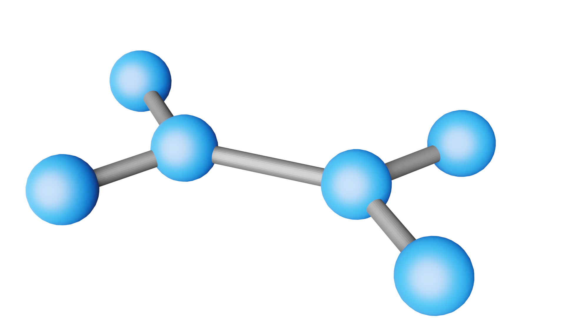
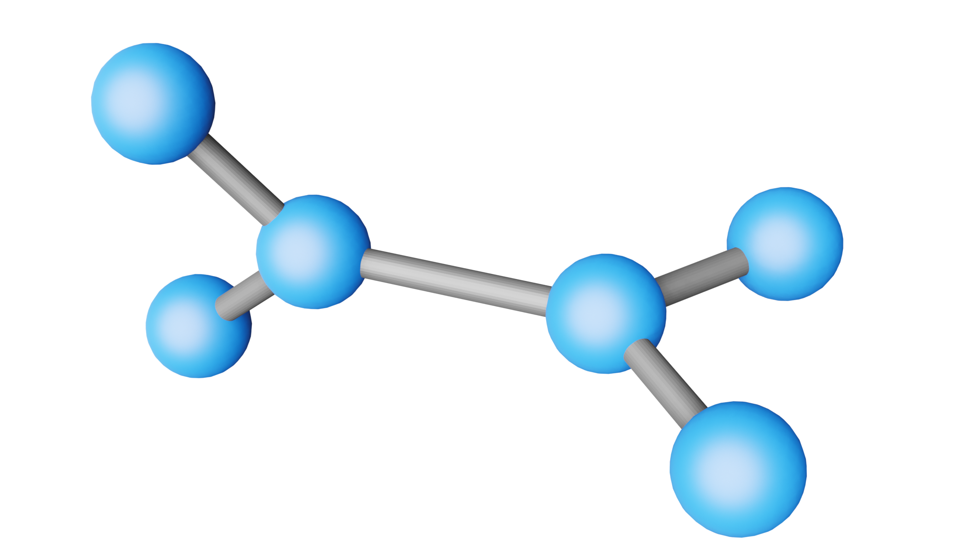
The architectures we present are also able to deal with some local symmetries. Namely, the DGN and AGN preserve local distances and angles respectively where a suitable subgraph must be defined. As an example consider a transformation that rotates only some nodes of a graph; all nodes which are in the neighbourhoods of the nodes will, in the angular architecture, have their angles preserved, and in the distance-preserving architecture, the distances between nodes will be preserved. A pertinent use-case for such a symmetry is that of molecular conformations, where the spatial arrangement of the atoms can be interconverted by rotations about formally single bonds, as shown in Figure 1). The AGN would be equivariant to such a transformation at the level of the two distinct subgraphs separated by the bond in question, thus enabling one to learn conformation-invariant properties.

4.2 Comparing and extending the two architectures

As mentioned, the two architectures we presented are partially overlapping in terms of equivariance features. Both of them are equivariant to the $E(n)$ group but the first one can deal with non-orthogonal transformations that preserve the distance between neighbouring nodes (such as with the Hoberman sphere) and the angular one is equivariant to the conformal group which allows to non-orthogonal transformations that preserve angles but not distances (see Figure 2).

The distance equivariant graph network can be equipped with a sense of scale equivariance through an input scaling layer that makes it invariant to the conformal orthogonal group. Let $\gamma=\alpha/\max_{(i,j)\in\mathcal{E}}\|\mathbf{x}_{i}-\mathbf{x}_{j}\|$ for some $\alpha\in\mathbb{R}$, where we identify $\gamma$ as satisfying the dilation condition required under the conformal orthogonal group. Then, conformal orthogonal invariance can simply be obtained by computing scale-normalised coordinates $\tilde{\mathbf{x}}_{i}=\gamma\mathbf{x}_{i}$ and using them as the coordinates in (3).

Introducing coordinate scaling therefore enables the distance equivariant graph network to be scale equivariant, under the condition that all transformations remain orthogonal. With the AGN, we can relax this condition and be equivariant under the full conformal group. This larger group equivariance enables us to work with very powerful transformations on data, which can also be dangerous. For example, if the scale is an important property of the dataset, the AGN will not recognise it and so will learn incorrect information about the data. Similarly, one must also not use the DGN blindly and irrespective of the properties of the dataset; as the architecture is equivariant to transformations that preserve distance between neighbouring nodes but not angles it is able to, for example, map a square onto a line. The two architectures we presented can be also combined together at the price of losing some features, while generalising to both distance and angle preserving transformations.

Figure 2: Equivariance of the two networks. The green/red square denotes the base graph and the blue/black ones alternative coordinate embeddings, equivariant for the DGN (red) or AGN (green).

5 Related work

The study and formulation of group equivariant neural networks have flourished in the last years and they have proven to be extremely powerful in many tasks. The first example is probably that of convolutional neural networks (LeCun et al., 1990), which are translation equivariant, thanks to the convolution operation, and have led to breakthroughs in most vision tasks. CNNs have been generalised to exploit larger groups of symmetries. G-CNNs are proposed in (Cohen and Welling, 2016) to deal with more general symmetries, including rotations and translations, and extended in (Bekkers, 2020; Finzi et al., 2020) to deal with Lie groups. Equivariance to arbitrary symmetry groups can be achieved via self-attention mechanisms in (Romero and Cordonnier, 2021). Continuous convolutions are used in SchNet (Schütt et al., 2017) to achieve $E(n)$ invariance, and $SE(3)$ equivariance is achieved in Thomas et al. (2018a) via the use of spherical harmonics. The drawback of many of these methods is their limited applicability due to computational complexity.

There has been some work on constructing general MLPs that are equivariant to different groups; a layer equivariant to general matrix groups is presented in Finzi et al. (2021), whilst equivariance to the Lorentz group for physics applications has recently been explored (Bogatskiy et al., 2020). Further applications include (Mattheakis et al., 2019), where physical symmetries are embedded in neural networks via embedding physical constraints in the structure of the network, and in (Barenboim et al., 2021) where the ability of neural networks to discover and learn symmetries in data is explored.

Graph neural networks are, by construction, permutation equivariant (Scarselli et al., 2008; Battaglia et al., 2018). Recently, there has been a lot of work on building equivariance to other interesting groups in GNNs. There has been particular interest in the Euclidean group with results for the subgroups $SE(3)$ and $E(3)$ obtained in (Thomas et al., 2018b; Fuchs et al., 2020; Köhler et al., 2020; Finzi et al., 2020; Batzner et al., 2021; Yang et al., 2020). Extending these architectures, an $E(n)$ equivariant message passing convolutional graph layer is proposed in (Satorras et al., 2021), leading to state of the art results in a variety of tasks, including $n$-body particle systems simulations and molecular property predictions. A similar idea has been also proposed in (Slade and Farina, 2021), where a general $E(n)$ equivariant GNN is presented, and in (Horie et al., 2021), in which equivariance to isometric transformations is considered. These $E(n)$ equivariant networks can be seen as special instances of our distance equivariant architecture, where particular aggregation functions are applied and a particular choice is made for the distance preserving map $\psi^{x}$ (see Appendix E). In (Satorras et al., 2021), for example, the map $\psi^{x}$ is chosen so that relative distances between all possible pairs of node in the graph are preserved, thus allowing only for rigid transformations in $E(n)$.

Angular information is used in (Smith et al., 2017) but no attention is explicitly paid to equivariance. DimeNET is proposed in (Klicpera et al., 2020), where both distance and angle embeddings computed through embeddings in novel orthogonal basis functions are used in a message passing graph network to achieve equivariance. State of the art results are obtained on molecular property and dynamics prediction datasets. We note, however, that while DimeNET produces state of the art results, it is restricted to atomic data, due to the requirement of Gaussian radial and Bessel functions as the basis representations. Additionally, angular embeddings computed in the isometric invariant layer in (Horie et al., 2021) corresponds to the extraction of both relative distances and angles of each pair of vertices. Again, these approaches are special instances of our networks where particular aggregation and learnable functions or hand engineered distance and/or angle embeddings are used (see Appendix E). In this sense, our network is unconstrained and can learn what it needs. Moreover, thanks to its general form it can achieve equivariance to the conformal group (and more) which, to the best of our knowledge, does not hold for known architectures.

To summarise, most of the existent equivariant graph architecture are at most equivariant to the Euclidean group (represented as the intersection set in Figure 2), while the architectures proposed here are, in their general form, equivariant to more much general transformations.

6 Experimental results

In this section we give an insight into the performance of the architectures we proposed and on their limitations. First, we demonstrate that perfect generalisation to unseen data can be achieved on datasets with a large number of symmetries, possibly accompanied by a faster convergence rate (as shown for QM9 in Appendix F.4). Then, we show that, when used on datasets with few symmetries, using our architectures can be counterproductive. In general, when the right symmetries are present, equivariant architectures experience both increased accuracy and convergence speed, as demonstrated by state of the art results obtained on a number of tasks by architectures that can be obtained as particular instances of the ones proposed here. Examples include $n$-body system dynamics prediction, molecular dynamics and molecular property prediction tasks (Satorras et al., 2021; Klicpera et al., 2020; Horie et al., 2021).

			test accuracy
block	$\rho$	train acc	Orthogonal	Orthogonal + dilation	Non-orthogonal ($\mu=0.5$)	Non-orthogonal ($\mu=1.5$)	Non-orthogonal ($\mu=3.0$)
AGN	mean	$1$	$\bm{1}$	$\bm{1}$	$\bm{1}$	$\bm{1}$	$\bm{0.96\pm 0.04}$
AGN	sum	$1$	$\bm{1}$	$\bm{1}$	$\bm{1}$	$\bm{1}$	$\bm{1}$
SDGN	mean	$0.2$	$0.2$	$0.2$	$0.2$	$0.2$	$0.2$
SDGN	sum	$1$	$\bm{1}$	$\bm{1}$	$\bm{1}$	$0.91\pm 0.07$	$0.83\pm 0.11$
DGN	mean	$1$	$\bm{1}$	$0.28\pm 0.02$	$0.20\pm 0.01$	$0.28\pm 0.01$	$0.30\pm 0.01$
DGN∗	sum	$1$	$\bm{1}$	$0.34\pm 0.05$	$0.28\pm 0.12$	$0.36\pm 0.07$	$0.35\pm 0.04$
GN	mean	$1$	$0.26\pm 0.03$	$0.25\pm 0.03$	$0.27\pm 0.04$	$0.25\pm 0.03$	$0.24\pm 0.04$
GN	sum	$1$	$0.40\pm 0.05$	$0.36\pm 0.04$	$0.32\pm 0.05$	$0.38\pm 0.07$	$0.35\pm 0.05$

Table 1: Polytopes classification: training and test accuracy (mean $\pm$ standard deviation over $10$ runs) for $n=3$, for different transformations in the test set. ^∗ equivalent to (Satorras et al., 2021).

6.1 Polytopes classification

We consider a $n$-dimensional polytopes classification problems for $n=3,4,5$. The datasets are composed of graph representations of polytopes and the number of classes varies with $n$. For $n=3$, simplexes, hypercubes, orthoplexes, dodecahedra and icosahedra are considered. Details and results for other values of $n$ are reported in Appendix F.2. The training dataset consists of a single graph per regular polytope (specified in terms of node coordinates and list of edges) while the test set is composed of randomly transformed versions of those in the training set, whose coordinates are obtained as $\tilde{\mathbf{x}}_{i}=\gamma A\mathbf{x}_{i}+q$ for some $\gamma\in\mathbb{R}$, $A\in\mathbb{R}^{n\times n}$ and $q\in\mathbb{R}^{n}$. We compare graph networks built with AGN, DGN and standard blocks. The DGN block is also combined with a scaling layer (SDGN) as in Section 4.2 to obtain equivariance to dilations. Mean and sum aggregation functions $\rho$ are considered. Results are reported in Table 1 for $\psi^{x}$ chosen as the identity function, i.e., $\mathbf{x}_{i}^{+}=\mathbf{x}_{i}$ (a more complex one is also considered in Appendix F.2).

We note that all models reach a perfect accuracy on the training set, except the SDGN with mean aggregation function, which is not able to distinguish any polytopes. If one changes the coordinate update function $\psi^{x}$ the accuracy reaches $0.8$ and only simplexes and orthoplexes are confounded. Adding (non all identical) node attributes to the graphs in addition to node coordinates enables all polytopes to be discerned. This behaviour is caused by the combination of the mean aggregation function and the scaling layer which makes the information propagated through the network be the same for all polytopes. When only orthogonal transformations are performed in the test set (i.e., $A^{\top}A=I$, $\gamma=1$) AGN, DGN and SDGN (with sum aggregation) perfectly generalise to unseen data. However, as expected, when also adding dilations (i.e., $A^{\top}A=\gamma I$, $\gamma\in\mathbb{R}$), only AGN and SDGN (with sum aggregation) can generalise well. Finally, when adding random non-orthogonal transformations (i.e., $\mu=\text{E}[\|A^{\top}A-I\|_{F}]>0$, $\gamma\in\mathbb{R}$), something possibly unexpected can be seen to happen. The AGN (and partially also the SDGN) perfectly generalises to unseen polytopes whose angles have not been preserved (due to the non-orthogonality of $A$). This is probably due to the network having learnt to distinguish polytopes based on the sum (or mean) of their angles which is preserved under non-orthogonal transformations due to the Gram–Euler theorem. While this behaviour turns out to be useful in the task at hand, one can easily envisage cases in which it may cause issues.

6.2 Benchmark datasets

Now we consider benchmark datasets from (Dwivedi et al., 2020) for which node coordinates are provided. In particular, we consider MNIST, CIFAR10 as graph classification problems and TSP as an edge classification one. While, when treated as images, MNIST and CIFAR10 are usually examples of datasets containing symmetries, in their graph representation such symmetries are mostly lost. Furthermore, in TSP there are no apparent symmetries in the dataset. In these cases, as one may expect, using an equivariant network would not produce any benefits. Rather, as we show, negative effects can appear.

We trained our models and a standard GNN on these datasets. All models have roughly the same number of parameters and the results are reported in Table 2. As can be seen, treating node coordinates as if they can posses some symmetric between among different samples turns out to be counterproductive both in terms of convergence speed and accuracy. In particular we see that while the standard GN has the best performance, the DGN is slightly better than the AGN. This is probably due to the fact that, while some non-orthogonal transformations mostly preserving local distances may be present in the dataset, angle preserving ones are much more rare. On TSP in particular, using angle related properties results in a significant drop in performance.

	MNIST		CIFAR10		TSP
block	train acc	test acc	train acc	test acc	train F1 (positive)	test F1 (positive)
AGN	$0.943\pm 0.004$	$0.932\pm 0.004$	$0.644\pm 0.004$	$0.590\pm 0.004$	$0.632\pm 0.011$	$0.681\pm 0.020$
DGN	$0.957\pm 0.001$	$0.945\pm 0.006$	$0.657\pm 0.004$	$0.592\pm 0.002$	$0.748\pm 0.013$	$0.771\pm 0.014$
GN	$\bm{0.982\pm 0.001}$	$\bm{0.977\pm 0.002}$	$\bm{0.719\pm 0.007}$	$\bm{0.657\pm 0.001}$	$\bm{0.772\pm 0.041}$	$\bm{0.793\pm 0.033}$

Table 2: Benchmark datasets. Train and test accuracy are reported for MNIST and CIFAR10. For TSP, due to the high class unbalance, the train and test F1 score for the positive class is reported.

6.2.1 Computational complexity

All the experiments have been run on an NVIDIA V100 GPU. The average time required for each training step (i.e., forward pass, back-propagation and optimiser step for a batch of data) is reported in Table 3, normalised with respect to the batch-size. Using the scaling layer for the DGN drastically increase the computational complexity. Moreover, it can be seen that while the AGN and DGN have similar complexities for dataset in which the number of edges (and hence angles) is relatively low, when graphs are (nearly) complete (like in TSP) or highly connected, the AGN has an overhead with respect to the DGN (due to the need of updated and computing angles in addition to edges).

	Time per training step (ms)
	polytopes (n=3)	polytopes (n=4)	polytopes (n=5)	MNIST	CIFAR10	TSP	QM9
batch-size	5	6	3	128	128	8	512
AGN	3.8	3.8	6.3	1.17	1.64	35	0.23
SDGN	5	14.5	8	7.81	12.5	-	-
DGN	3.8	3.7	6.3	0.78	1.09	16	0.19
GN	3	3	5	0.77	1.02	14	0.16

Table 3: Time per training step in the various experiments, normalised with respect to the batch-size.

7 Conclusion

In this paper we have presented novel deep learning architectures which are equivariant to distance and angle preserving transformations in graph coordinate embeddings. In particular, we have shown equivariance to the $E(n)$, $\text{CO}(\mathbb{R}^{n},\mathcal{Q})$ and $\text{Conf}(\mathbb{R}^{n,0})$ groups in addition to permutation equivariance. Equivariance to local symmetries can also be achieved when the different transformations are applied to suitable subgraphs. We have applied our models to a synthetic dataset composed of $n$-dimensional regular polytopes as well as to several benchmark datasets. We have shown that the architectures we propose are significantly more accurate and data efficient than a standard graph network on datasets where there are large numbers of symmetries in the data. We also explicitly show examples where our architecture produces unexpected results or would not be applicable, due to a lack of symmetry in the data.

Appendix A $E(n)$ equivariance of $\|\mathbf{x}_{i}-\mathbf{x}_{j}\|_{2}^{2}$

To show that $\|\mathbf{x}_{i}-\mathbf{x}_{j}\|_{2}^{2}$ is equivariant under $E(n)$, it is sufficient to see that, under translation, one has

$$\mathbf{x}\to\mathbf{x}^{+}=\mathbf{x}+\mathbf{z},\quad\mathbf{z}\in\mathbb{E}^{n}\,,$$

while under rotation

$$\mathbf{x}\to\mathbf{x}^{+}=Q\mathbf{x},\quad Q\in O(n)\,.$$

Now, by using the above relations and the fact that $E(n)$ is the semidirect product of $T(n)$ and $O(n)$, it is easy to show that $\|\mathbf{x}_{i}-\mathbf{x}_{j}\|_{2}^{2}$ is equivariant under $E(n)$ since

$$\|\mathbf{x}_{i}-\mathbf{x}_{j}\|_{2}^{2}\to\|\mathbf{x}_{i}^{+}-\mathbf{x}_{j}^{+}\|_{2}^{2} =(Q(\mathbf{x}_{i}+\mathbf{z})-Q(\mathbf{x}_{j}+\mathbf{z}))^{\top}(Q(\mathbf{x}_{i}+\mathbf{z})-Q(\mathbf{x}_{j}+\mathbf{z}))$$ (7a)

$$=(Q\mathbf{x}_{i}-Q\mathbf{x}_{j})^{\top}(Q\mathbf{x}_{i}-Q\mathbf{x}_{j})$$ (7b)

$$=(\mathbf{x}_{i}-\mathbf{x}_{j})^{\top}Q^{\top}Q(\mathbf{x}_{i}-\mathbf{x}_{j})$$ (7c)

$$=(\mathbf{x}_{i}-\mathbf{x}_{j})^{\top}(\mathbf{x}_{i}-\mathbf{x}_{j})\,,$$ (7d)

where we used the fact that $$Q^{\top}Q=I\,\forall Q\in O(n)$$.

Appendix B Equivariance under the conformal orthogonal group

In this section we will derive the result from Section 2.1.2 in the main text, that dilations and orthogonal rotations are transformations under $\text{CO}(\mathbb{R}^{n},\mathcal{Q})$. The group is defined for a vector space $V$ with a quadratic form $\mathcal{Q}$. The group contains the linear transformations $\varphi:\mathcal{T}\to V$. The group action is defined as

$$\mathcal{Q}(\mathcal{T}x)=\gamma^{2}\mathcal{Q}(x)\,,$$ (8)

where $\mathcal{T}$ is the set of linear transformations that we need to define and $\gamma$ is a scalar. For our purposes, we can consider a positive-definite quadratic form on $\mathbb{R}^{n}$; as we restrict our discussion to Euclidean space then the relevant quadratic form is

$$\mathcal{Q}=\sum_{i}x_{i}^{2}\,,$$ (9)

and so inserting (9) into (8) we have the condition

$$\sum_{i}(\mathcal{T}x_{i})^{2}=\gamma^{2}\sum_{i}x_{i}^{2}\,.$$

If we consider, as above, an orthogonal transformation $Q$, and in addition, a dilation $x_{i}\to\gamma x_{i}$, then it is simple to show that, with $\mathcal{T}=\gamma Q$

$$\sum_{i}(\gamma Qx_{i})^{2} =\gamma^{2}Q^{\top}Q\sum_{i}x_{i}^{2}=\gamma^{2}\sum_{i}x_{i}^{2}\,.$$

Appendix C Relative distance and angle preserving maps

Many different relative distance and/or angle preserving maps to be used in the coordinate update can be obtained in different ways, eventually requiring further assumptions on the data.

The simplest one is the identity function

$$\mathbf{x}_{i}^{+}=\psi(i,\mathcal{G}_{X})=\mathbf{x}_{i}$$ (10)

which keeps the coordinates unchanged during the update step. In this case both relative distances and angles are trivially preserved. Updating all the coordinates in the same way also trivially preserves both relative distances and angles. Examples include

$$\mathbf{x}_{i}^{+} =a\mathbf{x}_{i}, a\in\mathbb{R},$$

$$\mathbf{x}_{i}^{+} =\mathbf{x}_{i}+\mathbf{a}, \mathbf{a}\in\mathbb{R}^{n_{x}}$$

$$\mathbf{x}_{i}^{+} =Q\mathbf{x}_{i}+\mathbf{a}, Q\in\mathbb{R}^{n_{x}\times n_{x}},Q^{\top}Q=I,\mathbf{a}\in\mathbb{R}^{n_{x}}$$

where $a,\mathbf{a},Q$ can be learnable parameters or parametric functions of other network parameters, e.g., $\mathbf{a}=\phi^{x}(\mathbf{u})$. The matrix $Q$ can also be non orthogonal, provided that the obtained transformation preserves distances or angles.

Devising more complex forms for $\psi$ for arbitrary coordinate embeddings $X$, $Y$ satisfying the relative distance or angle preserving property, is quite tricky and further assumptions are in general required. To see this, consider a relative distance preserving transformation. Any transformation $X\to Y$, such that $\|\mathbf{x}_{i}-\mathbf{x}_{j}\|^{2}=\|\mathbf{y}_{i}-\mathbf{y}_{j}\|^{2}$, can be obtained as $\mathbf{x}_{i}=\gamma_{i}A_{i}\mathbf{y}_{i}+\mathbf{q}_{i}$, where $\gamma_{i}$, $A_{i}$ and $\mathbf{q}_{i}$, $i\in\mathcal{V}$, are solutions to the system

$$\|\gamma_{i}A_{i}\mathbf{y}_{i}+\mathbf{q}_{i}-\gamma_{j}A_{j}\mathbf{y}_{j}+\mathbf{q}_{j}\|^{2}=\|\mathbf{y}_{i}-\mathbf{y}_{j}\|^{2},\quad(i,j)\in\mathcal{E}.$$

with $\gamma_{i}\in\mathbb{R}$, $A_{i}^{\top}A_{i}=I$, $\mathbf{q}_{i}\in\mathbb{R}^{n_{n}}$, $\forall i\in\mathcal{V}$. In this general case, defining a (non trivial) map $\psi$ such that, after its application, one has $\|\mathbf{x}_{i}^{+}-\mathbf{x}_{j}^{+}\|^{2}=\|\mathbf{y}_{i}^{+}-\mathbf{y}_{j}^{+}\|^{2}\forall(i,j)\in\mathcal{E}$ is hard without any assumption on, at least, the topology of the graph $\mathcal{G}_{X}$ (or, equivalently $\mathcal{G}_{Y}$). A similar reasoning can be applied also to relative angle preserving maps.

If we restrict ourselves to the case in which $\gamma_{i}=\gamma$, $A_{i}=A$, $\mathbf{q}_{i}=\mathbf{q}$, $\forall i\in\mathcal{V}$, this results in $X$ being a Conformal orthogonal transformation of $Y$. In this case, a possible map $\psi$ is defined by

$$\mathbf{x}_{i}^{+}=\mathbf{x}_{i}+\sum_{j\in\mathcal{N}_{i}}a_{ji}(\mathbf{x}_{j}-\mathbf{x}_{i}).$$ (11)

with $a_{ji}$ possibly being a parametric function of node/edge/angle/global attributes, e.g., $a_{ji}=\phi^{x}\left(\mathbf{e}_{ji}^{+},\mathbf{v}_{j}^{+},\mathbf{v}_{i}^{+},\mathbf{u}\right)$. Now we show that (11) is both relative distance and angle preserving. For the sake of notation, we assume $\gamma=1$, however the same arguments can be applied when $\gamma\neq 1$.

Relative distance preservation of (11)

To show that (11) satisfies the definition of a distance-preserving map it is sufficient to show that, since $\mathbf{x}_{i}=A\mathbf{y}_{i}+q$, one has

$$\mathbf{x}_{i}^{+} =\mathbf{x}_{i}+\sum_{j\in\mathcal{N}_{i}}a_{ij}(\mathbf{x}_{j}-\mathbf{x}_{i})$$

$$=A\mathbf{y}_{i}+\mathbf{q}+\sum_{j\in\mathcal{N}_{i}}a_{ij}(A\mathbf{x}_{j}+\mathbf{q}-A\mathbf{x}_{i}-\mathbf{q})$$

$$=A\mathbf{y}_{i}+\mathbf{q}+\sum_{j\in\mathcal{N}_{i}}a_{ij}(A\mathbf{x}_{j}-A\mathbf{x}_{i})$$

$$=A\left[\mathbf{y}_{i}+\sum_{j\in\mathcal{N}_{i}}a_{ij}(\mathbf{x}_{j}-\mathbf{x}_{i})\right]+\mathbf{q}$$

$$=A\mathbf{y}_{i}^{+}+\mathbf{q}$$ (12)

which implies

$$\|\mathbf{x}_{i}^{+}-\mathbf{x}_{j}^{+}\|^{2} =\|A\mathbf{y}_{i}^{+}+\mathbf{q}-A\mathbf{y}_{j}^{+}-\mathbf{q}\|^{2}$$

$$=\|A(\mathbf{y}_{i}^{+}-\mathbf{y}_{j}^{+})\|^{2}$$

$$=(\mathbf{y}_{i}^{+}-\mathbf{y}_{j}^{+})^{\top}A^{\top}A(\mathbf{y}_{i}^{+}-\mathbf{y}_{j}^{+})$$

$$=\|\mathbf{y}_{i}^{+}-\mathbf{y}_{j}^{+}\|^{2}$$

where in the last line we used the fact that $A^{\top}A=I$.

Relative angle preservation of (11)

While (12) implies that angles are preserved since $\mathbf{x}_{i}$ is an $E(n)$ transformation of $\mathbf{y}_{i}$, one can show this explicitly by recalling that the angle between two vectors $\mathbf{x}_{j}-\mathbf{x}_{i}$ and $\mathbf{x}_{k}-\mathbf{x}_{i}$ can be computed as

$$\text{cos}\angle(\mathbf{x}_{j},\mathbf{x}_{i},\mathbf{x}_{k}) =\frac{(\mathbf{x}_{j}-\mathbf{x}_{i})^{\top}(\mathbf{x}_{k}-\mathbf{x}_{i})}{\|\mathbf{x}_{j}-\mathbf{x}_{i}\|\|\mathbf{x}_{k}-\mathbf{x}_{i}\|}$$

Then, one has

$$\frac{(\mathbf{x}_{j}^{+}-\mathbf{x}_{i}^{+})^{\top}(\mathbf{x}_{k}^{+}-\mathbf{x}_{i}^{+})}{\|\mathbf{x}_{j}^{+}-\mathbf{x}_{i}^{+}\|\|\mathbf{x}_{k}^{+}-\mathbf{x}_{i}^{+}\|} =\frac{(A\mathbf{y}_{j}^{+}+\mathbf{q}-A\mathbf{y}_{i}^{+}-\mathbf{q})^{\top}(A\mathbf{y}_{k}^{+}+\mathbf{q}-A\mathbf{y}_{i}^{+}-\mathbf{q})}{\|A\mathbf{y}_{j}^{+}+\mathbf{q}-A\mathbf{y}_{i}^{+}-\mathbf{q}\|\|A\mathbf{y}_{k}^{+}+\mathbf{q}-A\mathbf{y}_{i}^{+}-\mathbf{q}\|}$$

$$=\frac{(A\mathbf{y}_{j}^{+}-A\mathbf{y}_{i}^{+})^{\top}(A\mathbf{y}_{k}^{+}-A\mathbf{y}_{i}^{+})}{\|A\mathbf{y}_{j}^{+}-A\mathbf{y}_{i}^{+}\|\|A\mathbf{y}_{k}^{+}-A\mathbf{y}_{i}^{+}\|}$$

$$=\frac{(\mathbf{y}_{j}^{+}-\mathbf{y}_{i}^{+})^{\top}A^{\top}A(\mathbf{y}_{k}^{+}-\mathbf{y}_{i}^{+})}{\sqrt{(\mathbf{y}_{j}^{+}-\mathbf{y}_{i}^{+})^{\top}A^{\top}A(\mathbf{y}_{j}^{+}-\mathbf{y}_{i}^{+})}\sqrt{(\mathbf{y}_{k}^{+}-\mathbf{y}_{i}^{+})^{\top}A^{\top}A(\mathbf{y}_{k}^{+}-\mathbf{y}_{i}^{+})}}$$

$$=\frac{(\mathbf{y}_{j}^{+}-\mathbf{y}_{i}^{+})^{\top}(\mathbf{y}_{k}^{+}-\mathbf{y}_{i}^{+})}{\|\mathbf{y}_{j}^{+}-\mathbf{y}_{i}^{+}\|\|\mathbf{y}_{k}^{+}-\mathbf{y}_{i}^{+}\|}$$

where in the last line we used the fact that $A^{\top}A=I$.

Local symmetry transformation of (11)

Suppose we have a local symmetry transformation, $A(\tilde{\mathbf{x}})$ which only acts on a subgraph $\tilde{\mathcal{G}}\in\mathcal{G}$, such that $\mathbf{v}=(\tilde{\mathbf{v}}_{1},\tilde{\mathbf{v}}_{2},\dots\tilde{\mathbf{v}}_{n},\mathbf{v}_{n+1},\dots\mathbf{v}_{m})$, and similarly for the edge, coordinate and angle features. The action of $A(\tilde{\mathbf{x}})$ is then

$$A(\tilde{\mathbf{x}})\mathbf{x} =\left(A(\tilde{\mathbf{x}})\tilde{\mathbf{x}}_{1},A(\tilde{\mathbf{x}})\tilde{\mathbf{x}}_{2},\dots A(\tilde{\mathbf{x}})\tilde{\mathbf{x}}_{n},A(\tilde{\mathbf{x}})\mathbf{x}_{n+1},\dots A(\tilde{\mathbf{x}})\mathbf{x}_{m}\right)$$

$$=\left(A(\tilde{\mathbf{x}})\tilde{\mathbf{x}}_{1},A(\tilde{\mathbf{x}})\tilde{\mathbf{x}}_{2},\dots A(\tilde{\mathbf{x}})\tilde{\mathbf{x}}_{n},\mathbf{x}_{n+1},\dots\mathbf{x}_{m}\right)\,.$$

By defining the 2 subgraphs as containing the coordinate features which are and are not affected by the symmetry transformation, we can therefore write a coordinate update (11) for both subgraphs; Eq. (11) for the $\mathbf{x}_{i}$ and, for the $\tilde{\mathbf{x}}_{i}$,

$$\tilde{\mathbf{x}}_{i}^{+}=\tilde{\mathbf{x}}_{i}+\sum_{j\in\mathcal{N}_{i}}a_{ji}(\tilde{\mathbf{x}}_{j}-\tilde{\mathbf{x}}_{i}).$$

We have shown above that this coordinate update preserves distances and angles for global group transformations; by defining the 2 subgraphs as above, we can promote the local symmetry transformation $A(\tilde{\mathbf{x}})$ to global transformations on subgraphs. Whilst here we have shown this for only 2 subgraphs, one can generalise the argument to any number of local transformations so long as the subgraphs are defined as above. As we have to subdivide the graph into subgraphs, we note that these local transformations cannot be defined arbitrarily as there must be a sense of a neighbourhood of nodes within each subgraph. A local transformation which affects unrelated nodes identically (which is a valid class of local symmetry) is not valid for this reason.

Appendix D Additional formulations

D.1 Alternative formulations for the angle preserving graph network

A number of variations can be proposed for the angle preserving graph network:

• Edge attributes can be used in angle updates

  $$\bm{\alpha}_{jik}^{+} =\phi^{\alpha}(\mathbf{v}_{i},\mathbf{v}_{j},\mathbf{v}_{k},\mathbf{e}_{ij},\mathbf{e}_{ik},\bm{\alpha}_{jik},\angle(\mathbf{x}_{j},\mathbf{x}_{i},\mathbf{x}_{k}),\mathbf{u}), \forall(j,i,k)\in\mathcal{A}.$$

• Relative distances can be used in the angle updates

  $$\bm{\alpha}_{jik}^{+}=\phi^{\alpha}(\dots,\|\mathbf{x}_{i}-\mathbf{x}_{j}\|_{2}^{2},\|\mathbf{x}_{i}-\mathbf{x}_{k}\|_{2}^{2},\angle(\mathbf{x}_{j},\mathbf{x}_{i},\mathbf{x}_{k}),\mathbf{u}),\,\,\,\, \forall(j,i,k)\in\mathcal{A}.$$

• Angle attributes can be used in edge updates

  $$\mathbf{e}_{ij}^{+} =\phi^{e}\big{(}\mathbf{e}_{ij},\mathbf{v}_{i},\mathbf{v}_{j},\rho^{\alpha\to e}\big{(}\{\bm{\alpha}_{ijk}^{+}\}_{k\in\mathcal{A}_{ij}}\big{)},\rho^{\alpha\to e}\big{(}\{\bm{\alpha}_{jik}^{+}\}_{k\in\mathcal{A}_{ji}}\big{)},\mathbf{u}\big{)}, \forall(i,j)\in\mathcal{E}$$

  where $\mathcal{A}_{ij}=\{k\mid(y,z,k)\in\mathcal{A},y=i,z=j\}$ is the set of angles whose first ray is defined by $(i,j)$.

• Angle embeddings can be ignored and node attributes can be updated with the angles themselves

  $$\mathbf{e}_{ji}^{+}=\phi^{e}\big{(}\mathbf{v}_{j},\mathbf{v}_{i},\mathbf{e}_{ji},\mathbf{u}\big{)}, \forall(j,i)\in\mathcal{E}$$

  $$\mathbf{v}_{i}^{+}=\phi^{v}\big{(}\mathbf{v}_{i},\rho^{e\to v}\big{(}\{\mathbf{e}_{ji}^{+}\}_{j\in\mathcal{N}_{i}}\big{)},\rho^{\alpha\to v}\big{(}\{\angle(\mathbf{x}_{j},\mathbf{x}_{i},\mathbf{x}_{k})\}_{(j,k)\in\mathcal{A}_{i}}\big{)},\mathbf{u}\big{)}, \forall i\in\mathcal{V}$$

  $$\mathbf{x}_{i}^{+}=\psi^{x}(i,\mathcal{G}_{X}), \forall i\in\mathcal{V}$$

  $$\mathbf{u}^{+}=\phi^{u}\big{(}\rho^{v\to u}(\{\mathbf{v}_{i}^{+}\}_{i\in\mathcal{V}}),\rho^{e\to u}(\{\mathbf{e}_{ji}^{+}\}_{(j,i)\in\mathcal{E}}),\mathbf{u}\big{)}.$$

D.2 Combined architecture

The DGN and AGN architectures can be combined in a single architecture. An example is

$$\bm{\alpha}_{jik}^{+}=\phi^{\alpha}(\mathbf{v}_{i},\mathbf{v}_{j},\mathbf{v}_{k},\bm{\alpha}_{jik},\angle(\mathbf{x}_{j},\mathbf{x}_{i},\mathbf{x}_{k}),\mathbf{u}), \forall(j,i,k)\in\mathcal{A}$$

$$\mathbf{e}_{ji}^{+}=\phi^{e}\big{(}\mathbf{v}_{j},\mathbf{v}_{i},\mathbf{e}_{ji},\|\mathbf{x}_{i}-\mathbf{x}_{j}\|_{2}^{2},\mathbf{u}\big{)}, \forall(j,i)\in\mathcal{E}$$

$$\mathbf{v}_{i}^{+}=\phi^{v}\big{(}\mathbf{v}_{i},\rho^{e\to v}\big{(}\{\mathbf{e}_{ji}^{+}\}_{j\in\mathcal{N}_{i}}\big{)},\rho^{\alpha\to v}\big{(}\{\bm{\alpha}_{jik}^{+}\}_{(j,k)\in\mathcal{A}_{i}}\big{)},\mathbf{u}\big{)}, \forall i\in\mathcal{V}$$

$$\mathbf{x}_{i}^{+}=\psi^{x}(i,\mathcal{G}_{X}), \forall i\in\mathcal{V}$$

$$\mathbf{u}^{+}=\phi^{u}\big{(}\rho^{v\to u}(\{\mathbf{v}_{i}^{+}\}_{i\in\mathcal{V}}),\rho^{e\to u}(\{\mathbf{e}_{ji}^{+}\}_{(j,i)\in\mathcal{E}}),\mathbf{u}\big{)}$$

where the global update can contain aggregated information about angles and distances and also the other updates can be generalised as shown above. This architecture is by construction equivariant to transformations in the coordinate embeddings for which both relative distances and angles are preserved.

Appendix E Obtaining other architectures as special instances

In this appendix we will represent some of the architectures discussed in the main text explicitly as instances of our architecture.

E.1 Dimenet [Klicpera et al., 2020]

Dimenet can be obtained from the AGN by considering edge and distance information in the angle update and using sum aggregation functions as

$$\bm{\alpha}_{ijk}^{+}=\phi^{\alpha}(\mathbf{e}_{ji},\|\mathbf{x}_{i}-\mathbf{x}_{j}\|_{2}^{2},\angle(\mathbf{x}_{i},\mathbf{x}_{j},\mathbf{x}_{k})),\,\,\,\, \forall(j,i,k)\in\mathcal{A}$$

$$\mathbf{e}_{ji}^{+}=\phi^{e}(\mathbf{e}_{ji},\sum_{i\in\mathcal{N}_{j}}\bm{\alpha}_{ijk}^{+}), \forall(j,i)\in\mathcal{E}$$

$$\mathbf{x}_{i}^{+}=\mathbf{x}_{i}, \forall i\in\mathcal{V}$$

$$\mathbf{v}_{i}^{+}=\phi^{v}\big{(}\mathbf{v}_{i},\sum_{j\in\mathcal{N}_{i}}\mathbf{e}_{ji}^{+}\big{)}, \forall i\in\mathcal{V}$$

where $\|\mathbf{x}_{i}-\mathbf{x}_{j}\|_{2}^{2}$ is defined represented within a set of orthogonal basis functions $e_{RBF}$ and the angles $\angle(\mathbf{x}_{i},\mathbf{x}_{j},\mathbf{x}_{k})$ within a basis defined as $\alpha_{SBF}$.

E.2 EGCN [Satorras et al., 2021]

The EGCN network is obtained from the DGN by selecting a specific form for the coordinate update function $\psi^{x}$ and using the sum aggregation function as $\phi^{e\to v}$, i.e.,

$$\mathbf{e}_{ji}^{+}=\phi^{e}\big{(}\mathbf{v}_{j},\mathbf{v}_{i},\mathbf{e}_{ji},\|\mathbf{x}_{i}-\mathbf{x}_{j}\|_{2}^{2}\big{)},\,\,\,\, \forall(j,i)\in\mathcal{E}$$

$$\mathbf{x}_{i}^{+}=\mathbf{x}_{i}+\sum_{j\neq i}(\mathbf{x}_{i}-\mathbf{x}_{j})\phi^{x}(\mathbf{e}_{ji}), \forall i\in\mathcal{V}$$

$$\mathbf{v}_{i}^{+}=\phi^{v}\big{(}\mathbf{v}_{i},\sum_{j\in\mathcal{N}_{i}}\mathbf{e}_{ji}^{+}\big{)}. \forall i\in\mathcal{V}$$

E.3 IsoGNN [Horie et al., 2021]

The IsoGNN architecture is defined for tensors of rank-$n$; to compare with the other architectures presented here, we show below the architecture for rank-1 tensors.

$$\mathbf{e}_{ji}^{+}=\left(\sum_{k,l\in\mathcal{V},k\neq l}\mathbf{T}_{ijkl}(\mathbf{x}_{k}-\mathbf{x}_{l})\right)\mathbf{v}_{j},\,\,\,\, \forall(j,i)\in\mathcal{E}$$

$$\mathbf{x}_{i}^{+}=\mathbf{x}_{i}, \forall i\in\mathcal{V}$$

$$\mathbf{v}_{i}^{+}=\phi^{v}\big{(}\mathbf{v}_{i},\sum_{j\in\mathcal{N}_{i}}\mathbf{e}_{ji}^{+}\big{)}, \forall i\in\mathcal{V}$$

where $\mathbf{T}_{ijkl}$ is an untrainable 2-dimensional matrix which is translation and rotation invariant, and determined offline from the data for each class of problem.

E.4 Other networks

Standard graph networks can be obtained from ours by skipping some updates or not considering equivariant information. Also other variants, including SchNet [Schütt et al., 2017] or TFN [Thomas et al., 2018a], can be cast as message passing architectures as shown in [Satorras et al., 2021].

Appendix F Additional experiments and implementation details

F.1 Common implementation details

The update functions of the networks are all implemented as MLPs. After the graph layers, the produced node embeddings are passed through another MLP, a global pooling layer and a final MLP with output dimension equal to the number of classes for graph classification tasks. For edge classification tasks (TSP), the architecture after the graph layers is a single MLP taking as input source and target nodes and predicting the class of each edge. Each network is trained starting from $10$ different initial conditions. The results in the tables contains the mean and standard deviation resulting from the $10$ initialisations.

F.2 Polytopes classification

F.2.1 Specific implementation details

All the MLPs have one hidden layer containing $64$ neurons and swish activation function. We used $2$ graph layers for AGN and $3$ for both the DGN and GN with embeddings in the hidden layers having dimension $32$. Aggregation functions and the pooling layer implements mean or sum operations (and are specified in the results’ tables). Adam [Kingma and Ba, 2014] is used to train the all the models with a learning rate $\alpha=0.001$ and no regularisation for $1000$ epochs. The batch-size is equal to the number of training samples (so $5,6,3$ respectively, for $n=3,4,5$).

F.2.2 Additional experiments for $n=3$

Coordinate update (11)

In the main paper we reported results for $n=3$ when the identity function (10) was used to perform the coordinate update. In Table 4 we report the results obtained when using (11) for the coordinate updates. As can be seen the main difference is that now SDGN has an accuracy of $0.8$ instead of $0.2$, being unable to correctly classify simplexes and orthoplexes. The other results are qualitatively similar.

			test accuracy
block	$\rho$	train acc	Orthogonal	Orthogonal + dilation	Non-orthogonal ($\mu=0.5$)	Non-orthogonal ($\mu=1.5$)	Non-orthogonal ($\mu=3.0$)
AGN	mean	$1$	$\bm{1}$	$\bm{1}$	$\bm{1}$	$\bm{1}$	$\bm{0.96\pm 0.04}$
AGN	sum	$1$	$\bm{1}$	$\bm{1}$	$\bm{1}$	$\bm{1}$	$\bm{1}$
SDGN	mean	$0.8$	$0.8$	$0.8$	$0.65\pm 0.05$	$0.40\pm 0.08$	$0.36\pm 0.06$
SDGN	sum	$1$	$\bm{1}$	$\bm{1}$	$0.89\pm 0.16$	$0.62\pm 0.24$	$0.60\pm 0.21$
DGN	mean	$1$	$\bm{1}$	$0.36\pm 0.02$	$0.25\pm 0.05$	$0.34\pm 0.02$	$0.30\pm 0.02$
DGN	sum	$1$	$\bm{1}$	$0.37\pm 0.04$	$0.31\pm 0.06$	$0.34\pm 0.04$	$0.32\pm 0.05$

Table 4: Polytopes classification: training and test accuracy (mean $\pm$ standard deviation over $10$ runs) for $n=3$, for different transformations in the test set.

Adding not all-identical node features

The experiments run so far used datasets containing only information about node coordinates and the presence of edges. If we add (not-all-identical) node features, then also SDGN with mean aggregation function is able to correctly classify all the polytopes. This happens thanks to the additional features breaking a symmetry making the graphs of the simplex and the orthoplex look identical to the SDGN layer.

Data efficiency

To emphasise the advantage of having a network that is able to exploit symmetries in the dataset in terms of data efficiency, we study how many samples in the training set are necessary for a standard GNN to reach reasonable generalisation performance. For the set of transformations we considered in the previous sections, we augmented the training set with $\{2,3,\dots,100\}$ randomly transformed (as in the respective test set) copies of each polytope. We trained a standard GNN on these augmented datasets and observed the resulting test accuracy after $1000$ epochs. Results are reported in Figure 3 for each set of transformations in terms of mean and standard deviation over $10$ random initialisations. It can be seen that $20$ samples per polytope may be sufficient when only orthogonal transformations are considered. Adding also dilations and non-orthogonal transformations further increases the number of data points that are required. This shows that while data augmentation can be successfully exploited, it is provably sub-optimal in terms of sample complexity [Mei et al., 2021] and architectures with built-in equivariance properties represent a more efficient strategy to consider.

Figure 3: Test accuracy vs samples per polytope in the training set for a standard GNN ($n=3$).

F.2.3 Experiments in higher dimensions

For $n=4$ simplexes, hypercubes, orthoplexes are considered along with $24$-, $120$- and $600$-cell polytopes. For $n>5$ only simplexes, hypercubes, orthoplexes are considered.

In Tables 5, 6 we report the results obtained for $n=4$ and $n=5$. Similarly as before, also for $n=4,5$ there are cases in which the DGN (or SDGN) is not able to distinguish between one or more polytopes. Moreover, for $n=5$ we note that SDGN with sum aggregation and $\phi^{x}$ as in (10) perfectly generalise to unseen data subject to non-orthogonal transformations, while the AGN with mean aggregation function has a drop in performance as $\mu$ increases.

				test accuracy
block	$\rho$	$\psi^{x}$	train acc	Orthogonal	Orthogonal + dilation	Non-orthogonal ($\mu=0.5$)	Non-orthogonal ($\mu=1.5$)	Non-orthogonal ($\mu=3.0$)
AGN	mean	(10)	$1$	$\bm{1}$	$\bm{1}$	$\bm{1}$	$\bm{1}$	$\bm{0.98\pm 0.04}$
AGN	mean	(11)	$1$	$\bm{1}$	$\bm{1}$	$\bm{1}$	$\bm{1}$	$\bm{0.97\pm 0.04}$
AGN	sum	(10)	$1$	$\bm{1}$	$\bm{1}$	$\bm{1}$	$\bm{1}$	$\bm{1}$
AGN	sum	(11)	$1$	$\bm{1}$	$\bm{1}$	$\bm{1}$	$\bm{1}$	$\bm{1}$
SDGN	mean	(10)	$0.17$	$0.17$	$0.17$	$0.17$	$0.17$	$0.17$
SDGN	mean	(11)	$1$	$\bm{1}$	$\bm{1}$	$0.57\pm 0.13$	$0.35\pm 0.10$	$0.27\pm 0.10$
SDGN	sum	(10)	$1$	$\bm{1}$	$\bm{1}$	$0.96\pm 0.03$	$0.85\pm 0.13$	$0.77\pm 0.17$
SDGN	sum	(11)	$1$	$\bm{1}$	$\bm{1}$	$0.82\pm 0.11$	$0.68\pm 0.14$	$0.65\pm 0.20$
DGN	mean	(10)	$0.83$	$0.83$	$0.31\pm 0.02$	$0.40\pm 0.03$	$0.32\pm 0.01$	$0.27\pm 0.04$
DGN	mean	(11)	$1$	$\bm{1}$	$0.34\pm 0.02$	$0.40\pm 0.04$	$0.38\pm 0.03$	$0.30\pm 0.03$
DGN	sum	(10)	$1$	$\bm{1}$	$0.50\pm 0.05$	$0.54\pm 0.08$	$0.45\pm 0.06$	$0.39\pm 0.08$
DGN	sum	(11)	$1$	$\bm{1}$	$0.50\pm 0.04$	$0.54\pm 0.04$	$0.52\pm 0.03$	$0.43\pm 0.06$
GN	mean	$-$	$1$	$0.14\pm 0.04$	$0.19\pm 0.05$	$0.21\pm 0.03$	$0.24\pm 0.02$	$0.22\pm 0.04$
GN	sum	$-$	$1$	$0.31\pm 0.07$	$0.31\pm 0.06$	$0.31\pm 0.05$	$0.33\pm 0.06$	$0.23\pm 0.04$

Table 5: Polytopes classification: training and test accuracy (mean $\pm$ standard deviation over $10$ runs) for $n=4$, for different transformations in the test set.

				test accuracy
block	$\rho$	$\psi^{x}$	train acc	Orthogonal	Orthogonal + dilation	Non-orthogonal ($\mu=0.5$)	Non-orthogonal ($\mu=1.5$)	Non-orthogonal ($\mu=3.0$)
AGN	mean	(10)	$1$	$\bm{1}$	$\bm{1}$	$\bm{0.99\pm 0.03}$	$0.86\pm 0.11$	$0.77\pm 0.13$
AGN	mean	(11)	$1$	$\bm{1}$	$\bm{1}$	$\bm{0.99\pm 0.03}$	$0.84\pm 0.11$	$0.75\pm 0.11$
AGN	sum	(10)	$1$	$\bm{1}$	$\bm{1}$	$\bm{1}$	$\bm{1}$	$\bm{1}$
AGN	sum	(11)	$1$	$\bm{1}$	$\bm{1}$	$\bm{1}$	$\bm{1}$	$\bm{1}$
SDGN	mean	(10)	$0.33$	$0.31\pm 0.08$	$0.31\pm 0.08$	$0.33$	$0.33$	$0.33$
SDGN	mean	(11)	$1$	$\bm{1}$	$\bm{1}$	$0.60\pm 0.25$	$0.48\pm 0.15$	$0.37\pm 0.10$
SDGN	sum	(10)	$1$	$\bm{1}$	$\bm{1}$	$\bm{1}$	$\bm{1}$	$\bm{1}$
SDGN	sum	(11)	$1$	$\bm{1}$	$\bm{1}$	$0.83\pm 0.16$	$0.75\pm 0.14$	$0.66\pm 0.18$
DGN	mean	(10)	$1$	$\bm{1}$	$0.49\pm 0.01$	$0.33\pm 0.00$	$0.49\pm 0.02$	$0.37\pm 0.01$
DGN	mean	(11)	$1$	$\bm{1}$	$0.51\pm 0.03$	$0.40\pm 0.04$	$0.41\pm 0.06$	$0.39\pm 0.05$
DGN	sum	(10)	$1$	$\bm{1}$	$0.53\pm 0.05$	$0.34\pm 0.05$	$0.51\pm 0.03$	$0.41\pm 0.10$
DGN	sum	(11)	$1$	$\bm{1}$	$0.57\pm 0.10$	$0.45\pm 0.12$	$0.54\pm 0.13$	$0.49\pm 0.10$
GN	mean	$-$	$1$	$0.30\pm 0.05$	$0.52\pm 0.08$	$0.34\pm 0.04$	$0.38\pm 0.08$	$0.43\pm 0.06$
GN	sum	$-$	$1$	$0.39\pm 0.07$	$0.49\pm 0.04$	$0.34\pm 0.08$	$0.40\pm 0.06$	$0.41\pm 0.08$

Table 6: Polytopes classification: training and test accuracy (mean $\pm$ standard deviation over $10$ runs) for $n=5$, for different transformations in the test set.

F.3 MNIST, CIFAR10, TSP

MNIST and CIFAR10 are classical image classification datasets converted into graphs using super-pixels and assigning the super-pixel coordinates as node coordinates and the intensity as node features. TSP (based on the Travelling Salesman Problem) tests link prediction on 2D Euclidean graphs to identify edges belonging to the optimal TSP solution given by the Concorde solver.

For this datasets we use the same splits as specified in [Dwivedi et al., 2020].

F.3.1 Specific implementation details

The MLPs have one hidden layer containing $64$ neurons, swish activation function and dropout layers with dropout rate $0.01$. We used $2$ graph layers for AGN and $3$ for both the DGN and GN with embeddings in the hidden layers having dimension $64$. Aggregation functions and the pooling layer implements sum operations. The models are trained with Adam with learning rate $\alpha=0.001$ and no regularisation for $100$ epochs. Batch-size $128$ is used for MNIST and CIFAR10, and $8$ for TSP.

F.4 Molecular property prediction - QM9

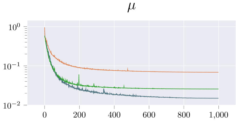
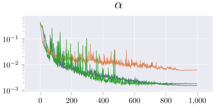
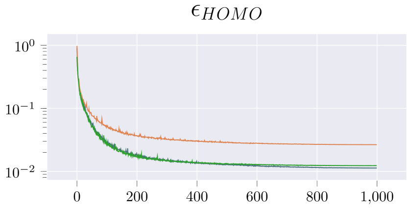
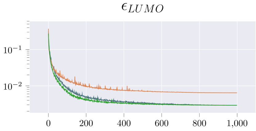
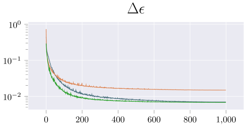
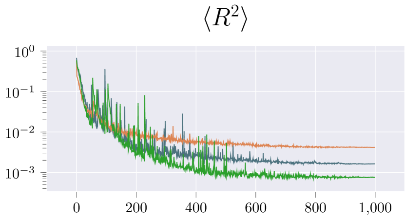
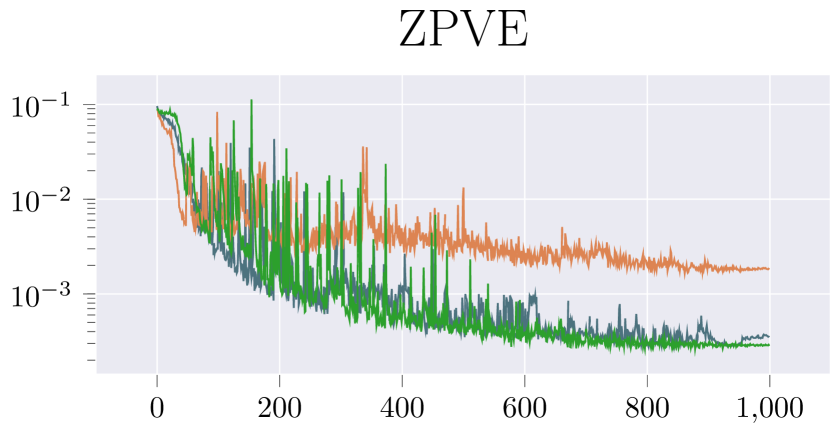
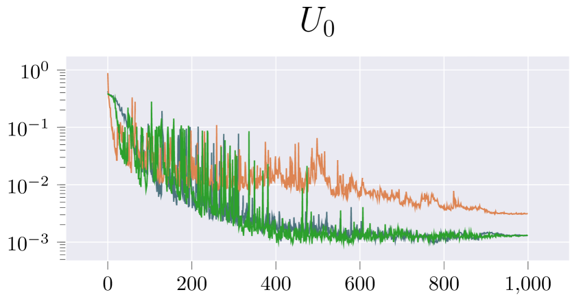
The QM9 dataset [Wu et al., 2017] is comprised of small molecules (hydrogen, carbon, nitrogen, oxygen, flourine) with the target properties being 12 chemical properties. As the target properties are equivariant to Euclidean transformations of the atoms’ coordinates, and also to the order in which atoms are processed, QM9 is an excellent benchmarking dataset for a GNN, especially if $E(n)$ equivariant. Indeed, state of the art results have been achieved on this dataset by EGCN and Dimenet [Satorras et al., 2021, Klicpera et al., 2020]. Here we show that, in addition to leading to better accuracy, employing equivariant networks give a significant improvement in convergence speed.

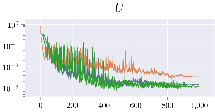
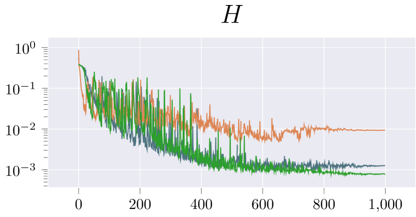
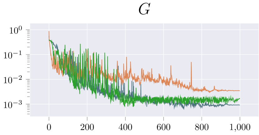
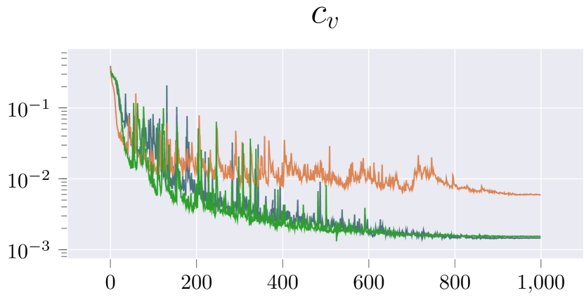
Figure 4 show the evolution of the mean squared error on the test set on all the target properties for both architectures. We see that both the AGN and DGN outperform the standard GN in two aspects; the model trains more rapidly, and also reaches a lower loss.

F.4.1 Specific implementation details

The QM9 dataset is composed of roughly 134k molecules: we used 100k for training and the remaining for testing. The AGN and DGN networks receive the embedding of the atomic properties as initial node features and the coordinates of each atom as coordinate features, while in the standard GNN they are stacked and provided as node features. Edge embeddings representing bond types are also provided.

The networks consist of 4 graph layers (3 for the AGN) with each MLP having 2 hidden layers of 128 nodes, swish activation function and dropout rate of 0.01. The node embeddings of the last graph layer are passed through an MLP, a global mean pooling layer and a last MLP to map them to the target chemical property. The last two MLPs each have a single hidden layer of 128 nodes, swish activation and dropout rate of 0.01. The target chemical properties are all standardised by subtracting the mean and dividing by the standard deviation for each target. The networks are trained for 1000 epochs using ADAM with a learning rate of $0.0005$ and mean squared error loss.

Figure 4: QM9: test MSE loss on the 12 target properties.

References

- Barenboim et al. [2021] Gabriela Barenboim, Johannes Hirn, and Veronica Sanz. Symmetry meets AI. arXiv preprint arXiv:2103.06115, 2021.
- Barnes et al. [1964] V. E. Barnes, P. L. Connolly, D. J. Crennell, B. B. Culwick, W. C. Delaney, W. B. Fowler, P. E. Hagerty, E. L. Hart, N. Horwitz, P. V. Hough, J. E. Jensen, J. K. Kopp, K. W. Lai, J. Leitner, J. L. Lloyd, G. W. London, T. W. Morris, Y. Oren, R. B. Palmer, A. G. Prodell, D. RadojičiĆ, D. C. Rahm, C. R. Richardson, N. P. Samios, J. R. Sanford, R. P. Shutt, J. R. Smith, D. L. Stonehill, R. C. Strand, A. M. Thorndike, M. S. Webster, W. J. Willis, and S. S. Yamamoto. Observation of a Hyperon with Strangeness Minus Three. Physical Review Letters, 12(8):204–206, 1964.
- Battaglia et al. [2018] Peter W. Battaglia, Jessica B. Hamrick, Victor Bapst, Alvaro Sanchez-Gonzalez, Vinicius Zambaldi, Mateusz Malinowski, Andrea Tacchetti, David Raposo, Adam Santoro, Ryan Faulkner, Caglar Gulcehre, Francis Song, Andrew Ballard, Justin Gilmer, George Dahl, Ashish Vaswani, Kelsey Allen, Charles Nash, Victoria Langston, Chris Dyer, Nicolas Heess, Daan Wierstra, Pushmeet Kohli, Matt Botvinick, Oriol Vinyals, Yujia Li, and Razvan Pascanu. Relational inductive biases, deep learning, and graph networks. 2018.
- Batzner et al. [2021] Simon Batzner, Tess E. Smidt, Lixin Sun, Jonathan P. Mailoa, Mordechai Kornbluth, Nicola Molinari, and Boris Kozinsky. Se(3)-equivariant graph neural networks for data-efficient and accurate interatomic potentials. 2021.
- Bekkers [2020] Erik J Bekkers. B-spline cnns on lie groups. In International Conference on Learning Representations, 2020.
- Bogatskiy et al. [2020] Alexander Bogatskiy, Brandon Anderson, Jan Offermann, Marwah Roussi, David Miller, and Risi Kondor. Lorentz group equivariant neural network for particle physics. In International Conference on Machine Learning, pages 992–1002. PMLR, 2020.
- Bronstein et al. [2021] Michael M Bronstein, Joan Bruna, Taco Cohen, and Petar Veličković. Geometric deep learning: Grids, groups, graphs, geodesics, and gauges. arXiv preprint arXiv:2104.13478, 2021.
- Cohen and Welling [2016] Taco Cohen and Max Welling. Group equivariant convolutional networks. In International conference on machine learning, pages 2990–2999. PMLR, 2016.
- Cranmer et al. [2020] Miles Cranmer, Alvaro Sanchez Gonzalez, Peter Battaglia, Rui Xu, Kyle Cranmer, David Spergel, and Shirley Ho. Discovering symbolic models from deep learning with inductive biases. In H. Larochelle, M. Ranzato, R. Hadsell, M. F. Balcan, and H. Lin, editors, Advances in Neural Information Processing Systems, volume 33, pages 17429–17442. Curran Associates, Inc., 2020.
- Dreyer and Qu [2021] Frédéric A. Dreyer and Huilin Qu. Jet tagging in the lund plane with graph networks, 2021.
- Dwivedi et al. [2020] Vijay Prakash Dwivedi, Chaitanya K Joshi, Thomas Laurent, Yoshua Bengio, and Xavier Bresson. Benchmarking graph neural networks. arXiv preprint arXiv:2003.00982, 2020.
- Finzi et al. [2020] Marc Finzi, Samuel Stanton, Pavel Izmailov, and Andrew Gordon Wilson. Generalizing convolutional neural networks for equivariance to lie groups on arbitrary continuous data. In International Conference on Machine Learning, pages 3165–3176. PMLR, 2020.
- Finzi et al. [2021] Marc Finzi, Max Welling, and Andrew Gordon Wilson. A practical method for constructing equivariant multilayer perceptrons for arbitrary matrix groups, 2021.
- Fuchs et al. [2020] Fabian Fuchs, Daniel Worrall, Volker Fischer, and Max Welling. Se(3)-transformers: 3d roto-translation equivariant attention networks. In H. Larochelle, M. Ranzato, R. Hadsell, M. F. Balcan, and H. Lin, editors, Advances in Neural Information Processing Systems, volume 33, pages 1970–1981. Curran Associates, Inc., 2020.
- Gell-Mann [1961] M Gell-Mann. The eightfold way: A theory of strong interaction symmetry. 3 1961.
- Gilmer et al. [2017] Justin Gilmer, Samuel S Schoenholz, Patrick F Riley, Oriol Vinyals, and George E Dahl. Neural message passing for quantum chemistry. In International Conference on Machine Learning, pages 1263–1272. PMLR, 2017.
- Gori et al. [2005] Marco Gori, Gabriele Monfardini, and Franco Scarselli. A new model for learning in graph domains. In Proceedings. 2005 IEEE International Joint Conference on Neural Networks, 2005., volume 2, pages 729–734. IEEE, 2005.
- Hamilton [2020] William L Hamilton. Graph representation learning. Synthesis Lectures on Artifical Intelligence and Machine Learning, 14(3):1–159, 2020.
- Horie et al. [2021] Masanobu Horie, Naoki Morita, Toshiaki Hishinuma, Yu Ihara, and Naoto Mitsume. Isometric transformation invariant and equivariant graph convolutional networks. In International Conference on Learning Representations, 2021.
- Kingma and Ba [2014] Diederik P. Kingma and Jimmy Ba. Adam: A method for stochastic optimization, 2014. cite arxiv:1412.6980Comment: Published as a conference paper at the 3rd International Conference for Learning Representations, San Diego, 2015.
- Kipf et al. [2018] Thomas Kipf, Ethan Fetaya, Kuan-Chieh Wang, Max Welling, and Richard Zemel. Neural relational inference for interacting systems. In International Conference on Machine Learning, pages 2688–2697. PMLR, 2018.
- Klicpera et al. [2020] Johannes Klicpera, Janek Groß, and Stephan Günnemann. Directional message passing for molecular graphs, 2020.
- Köhler et al. [2020] Jonas Köhler, Leon Klein, and Frank Noe. Equivariant flows: Exact likelihood generative learning for symmetric densities. In Hal Daumé III and Aarti Singh, editors, Proceedings of the 37th International Conference on Machine Learning, volume 119 of Proceedings of Machine Learning Research, pages 5361–5370. PMLR, 13–18 Jul 2020.
- LeCun et al. [1990] Yann LeCun, Bernhard E Boser, John S Denker, Donnie Henderson, Richard E Howard, Wayne E Hubbard, and Lawrence D Jackel. Handwritten digit recognition with a back-propagation network. In Advances in neural information processing systems, pages 396–404, 1990.
- Li et al. [2020] Yunzhu Li, Antonio Torralba, Anima Anandkumar, Dieter Fox, and Animesh Garg. Causal discovery in physical systems from videos. In H. Larochelle, M. Ranzato, R. Hadsell, M. F. Balcan, and H. Lin, editors, Advances in Neural Information Processing Systems, volume 33, pages 9180–9192. Curran Associates, Inc., 2020.
- Mattheakis et al. [2019] Marios Mattheakis, Pavlos Protopapas, David Sondak, Marco Di Giovanni, and Efthimios Kaxiras. Physical symmetries embedded in neural networks. arXiv preprint arXiv:1904.08991, 2019.
- Mei et al. [2021] Song Mei, Theodor Misiakiewicz, and Andrea Montanari. Learning with invariances in random features and kernel models. arXiv preprint arXiv:2102.13219, 2021.
- Peskin and Schroeder [1995] Michael E. Peskin and Daniel V. Schroeder. An Introduction to quantum field theory. Addison-Wesley, Reading, USA, 1995. ISBN 978-0-201-50397-5.
- Pfaff et al. [2021] Tobias Pfaff, Meire Fortunato, Alvaro Sanchez-Gonzalez, and Peter Battaglia. Learning mesh-based simulation with graph networks. In International Conference on Learning Representations, 2021.
- Romero and Cordonnier [2021] David W. Romero and Jean-Baptiste Cordonnier. Group equivariant stand-alone self-attention for vision. In International Conference on Learning Representations, 2021.
- Sanchez-Gonzalez et al. [2020] Alvaro Sanchez-Gonzalez, Jonathan Godwin, Tobias Pfaff, Rex Ying, Jure Leskovec, and Peter Battaglia. Learning to simulate complex physics with graph networks. In International Conference on Machine Learning, pages 8459–8468. PMLR, 2020.
- Satorras et al. [2021] Victor Garcia Satorras, Emiel Hoogeboom, and Max Welling. E(n) equivariant graph neural networks. 2021.
- Scarselli et al. [2008] Franco Scarselli, Marco Gori, Ah Chung Tsoi, Markus Hagenbuchner, and Gabriele Monfardini. The graph neural network model. IEEE transactions on neural networks, 20(1):61–80, 2008.
- Schütt et al. [2017] Kristof T Schütt, Farhad Arbabzadah, Stefan Chmiela, Klaus R Müller, and Alexandre Tkatchenko. Quantum-chemical insights from deep tensor neural networks. Nature communications, 8(1):1–8, 2017.
- Slade and Farina [2021] Emma Slade and Francesco Farina. Beyond permutation equivariance in graph networks, 2021.
- Smith et al. [2017] Justin S Smith, Olexandr Isayev, and Adrian E Roitberg. Ani-1: an extensible neural network potential with dft accuracy at force field computational cost. Chemical science, 8(4):3192–3203, 2017.
- Stokes et al. [2020] Jonathan M. Stokes, Kevin Yang, Kyle Swanson, Wengong Jin, Andres Cubillos-Ruiz, Nina M. Donghia, Craig R. MacNair, Shawn French, Lindsey A. Carfrae, Zohar Bloom-Ackermann, Victoria M. Tran, Anush Chiappino-Pepe, Ahmed H. Badran, Ian W. Andrews, Emma J. Chory, George M. Church, Eric D. Brown, Tommi S. Jaakkola, Regina Barzilay, and James J. Collins. A deep learning approach to antibiotic discovery. Cell, 180(4):688–702.e13, 2020.
- Thomas et al. [2018a] Nathaniel Thomas, Tess Smidt, Steven Kearnes, Lusann Yang, Li Li, Kai Kohlhoff, and Patrick Riley. Tensor field networks: Rotation- and translation-equivariant neural networks for 3d point clouds. 2018a.
- Thomas et al. [2018b] Nathaniel Thomas, Tess Smidt, Steven M. Kearnes, Lusann Yang, Li Li, Kai Kohlhoff, and Patrick Riley. Tensor field networks: Rotation- and translation-equivariant neural networks for 3d point clouds. CoRR, abs/1802.08219, 2018b.
- Wu et al. [2017] Zhenqin Wu, Bharath Ramsundar, Evan N. Feinberg, Joseph Gomes, Caleb Geniesse, Aneesh S. Pappu, Karl Leswing, and Vijay S. Pande. Moleculenet: A benchmark for molecular machine learning. CoRR, abs/1703.00564, 2017.
- Wu et al. [2020] Zonghan Wu, Shirui Pan, Fengwen Chen, Guodong Long, Chengqi Zhang, and S Yu Philip. A comprehensive survey on graph neural networks. IEEE transactions on neural networks and learning systems, 2020.
- Yang et al. [2020] Qin Yang, Chenglin Li, Wenrui Dai, Junni Zou, Guo-Jun Qi, and Hongkai Xiong. Rotation equivariant graph convolutional network for spherical image classification. In Proceedings of the IEEE/CVF Conference on Computer Vision and Pattern Recognition (CVPR), June 2020.
Appendix A equivariance of
To show that is equivariant under , it is sufficient to see that, under translation, one has