Existence and regularity for a system of porous medium equations with small cross-diffusion and nonlocal drifts

Abstract

We prove existence and Sobolev regularity of solutions of a nonlinear system of degenerate-parabolic PDEs with self- and cross-diffusion, transport/confinement and nonlocal interaction terms. The macroscopic system of PDEs is formally derived from a large particle system and models the evolution of an arbitrary number of species with quadratic porous-medium interactions in a bounded domain $\Omega$ in any spatial dimension. The cross interactions between different species are scaled by a parameter $\delta<1$, with the $\delta=0$ case corresponding to no interactions across species. A smallness condition on $\delta$ ensures existence of solutions up to an arbitrary time $T>0$ in a subspace of $L^{2}(0,T;H^{1}(\Omega))$. This is shown via a Schauder fixed point argument for a regularised system combined with a vanishing diffusivity approach. The behaviour of solutions for extreme values of $\delta$ is studied numerically.

1 Introduction, motivation and set-up

Partial differential equations involving nonlinear diffusion in combination with local or nonlocal transport are commonly used to model the macroscopic behaviour of a large number of agents or individuals in the natural, life, and social sciences. Systems involving many species or types of agents have been used to study multiple chemotactic populations in competition for nutrient [31, 38], tumour growth [32, 58, 61], pedestrian dynamics [7, 30], and opinion formation [37]. Further applications can be found in population biology [17, 29] and in semiconductor devices [28, 53].

In this paper we study a class of drift-diffusion systems taking the following form:

$$\partial_{t}u_{i}=\operatorname{div}\left[u_{i}(\nabla u_{i}+\nabla L_{i}(t,x,u_{i})+\delta F_{i}(t,x,u,\nabla u))\right],\qquad i=1,\dots,M,$$ (1)

where $u=(u_{1},\dots,u_{M})$ is a vector of non-negative functions defined on a bounded domain $Q_{T}=(0,T)\times\Omega$ describing the densities of $M$ subpopulations. The transport term $L_{i}$ models the presence of external forces and nonlocal self-interactions, $L_{i}(t,x,u_{i})=V_{i}(t,x)+\big{(}W_{i}*u_{i}(t,\cdot)\big{)}(x)$, while $F_{i}$ represents the interaction with the other species. The latter is of particular importance since it includes the contribution of cross-diffusion terms through the dependence on $\nabla u$.

One of the main features of (1) is that it can be used to describe cells sorting and the resulting pattern formation. This is a reorganisation process in which cells of different species—which in principle react differently to external forces such as chemical signal or attraction/repulsion with the other species—have the propensity to group together in a delimited region [46, 52, 63, 65]. This biological phenomenon can be also interpreted as the inhibition or activation of growth whenever two populations occupy the same habitat, which can be be attributed to volume or size constraints of the individual cells forming the different populations. In the seminal papers [9, 10, 11, 41] it was shown that segregation is induced by the presence of cross-diffusion terms. Nonlinear diffusion may also help in describing volume filling effects and in preventing blow-up in biological aggregation models, see [16, 21, 43, 57, 67].

The main goal of the present paper is to provide a well-posedness result for (1), which can be seen as a $\delta$-order perturbation of a set of $M$ decoupled drift-diffusion equations with degenerate diffusion of porous-media type and nonlocal interactions. One of the main difficulties for these systems is the lack of a suitable maximum principle, meaning that Sobolev estimates must be obtained in an alternative fashion. Under a smallness assumption on the perturbation parameter $\delta$, we are able to estimate each density in $L^{2}(0,T;H^{1}(\Omega))$, as well as the relative time derivatives in a dual Sobolev space. Such estimates allow us to show convergence of weak solutions for a proper regularised approximating sequence. The structure of the system and the numerical simulations indicate that the expected critical value for the $L^{2}(0,T;H^{1}(\Omega))$-framework is $\delta=1$. However, technical conditions impose a stricter bound on $\delta$. The $BV$ norm is the only norm expected to remain bounded as $\delta\to 1$.

The paper is organised as follows. In Section 1.1 we present a formal derivation of system (1) from a system of interacting particles. In Section 1.2 we provide the general set of assumptions and the statement of the main result, Theorem 1. We sketch the main steps in the strategy of the proof of the main result in Section 1.3, and we give a brief overview of different approaches and existing results in the literature in Section 1.4. Section 2 is devoted to the numerical investigation of a particular case of system (1), which helps to highlight the influence of the parameter $\delta$ in the time evolution of solutions and its norms. The remainder of the paper focuses on the proof of Theorem 1. In Section 3 we introduce a regularised system, providing existence, uniqueness and uniform estimates for these regularised solutions. In Section 4 we present a fixed point argument and show compactness properties for the solution map of the regularised system. Convergence of approximate solutions to weak solutions of system (1) is established in Section 5 through vanishing diffusivity. Appendix A collects some technical results used in the paper.

1.1 Model derivation

In this subsection we sketch a formal derivation of (1) starting from the interacting particle system with $M$ species, each composed of $N_{i}$ identical particles, $i=1,\dots,M$. To simplify the presentation, the derivation is shown for the case for $L_{i}(t,x,u_{i})\equiv V_{i}(x)$, that is, we drop the nonlocal interactions $W_{i}$ and the time-dependence, and a simple cross-diffusion term $F_{i}(t,x,u,\nabla u)\equiv\sum_{j=1,j\neq i}^{M}\nabla u_{j}$. The addition of nonlocal interactions and time is straightforward. We denote by $N$ the total number of particles, $N=\sum_{i}N_{i}$. We consider the following model:

$$\mathrm{d}X_{k}^{i}(t) =-\nabla V_{i}(X_{k}^{i})\mathrm{d}t-\sum_{j=1}^{M}\sum_{\begin{subarray}{c}\ell=1\\ (\ell,j)\neq(k,i)\end{subarray}}^{N_{i}}\nabla K_{ij}(X_{k}^{i}-X_{\ell}^{j})\mathrm{d}t,$$ (2a)

$$X_{k}^{i}(0) =\xi_{k}^{i},\qquad k=1,\dots,N_{i},$$ (2b)

where $$X_{k}^{i}(t) k i t \Omega\subset\mathbb{R}^{d} |\Omega|=1 \xi_{1}^{i},\dots,\xi_{N_{i}}^{i} u_{i,0}$$ is the position of the -th particle in the -th species at time , evolving in a bounded domain such that . Particles are initialised with independent and identically distributed random variables with the common probability density function .

Here $K_{ii}$ denotes the self-interaction potential in species $i$, and $K_{ij}$ denotes the cross-interaction potential between species $i$ and $j$. Note that $K_{ij}$ and $K_{ji}$ may differ to represent an asymmetric interaction between the two species. The potentials are assumed to be obtained from some fixed function $K_{0}$ by the scaling

$$K_{ij}(x)=\chi_{ij}K_{0}\left(\frac{|x|}{\varepsilon_{ij}}\right),$$ (3)

where the parameters $\chi_{ij}$ and $\varepsilon_{ij}$ represent the strength and the range of the interactions respectively, and depend on $N_{j}$ in a way that will be made specific later on. The scale-free potential $K_{0}:\mathbb{R}^{d}\to\mathbb{R}$ is a radial, nonnegative function whose gradient is locally Lipschitz outside the origin. Moreover, it is assumed that $\|K_{0}\|_{L^{1}}<\infty$. Without loss of generality, we set $\|K_{0}\|_{L^{1}}=1$.

Depending on $\chi$ and $\varepsilon$, one expects different limit equations [13]. For example, when the interactions are long range ($\varepsilon\sim 1$) and weak ($\chi\sim N^{-1}$), then one particle interacts on average with an order $N$ particles as $N\to\infty$ one recovers a mean-field limit for weakly interacting particles. In contrast, the case of moderately interacting particles corresponds to stronger but more localised interactions, so one particle interacts with fewer particles. As a result, one expects interactions to emerge as local terms in the limit equation.

We define the total interaction potential of the $i$-th species as

$$K_{i}(\vec{x})=\sum_{k=1}^{N_{i}}\bigg{[}\sum_{\ell>k}^{N_{i}}K_{ii}(x_{k}^{i}-x_{\ell}^{i})+\sum_{\begin{subarray}{c}j=1\\ j\neq i\end{subarray}}^{M}\sum_{\ell=1}^{N_{j}}K_{ij}(x_{k}^{i}-x_{\ell}^{j})\bigg{]}$$ (4)

where $\vec{x}=(x_{k}^{i})_{k=1,\dots,N_{i},i=1,\dots,M}$. Then the joint probability density $P_{N}(\vec{x},t)=\text{Prob}(X(t)=\vec{x})$ of $N$ particles evolving according to (2) satisfies the following equation

$$\partial_{t}P_{N}=\sum_{i=1}^{M}\sum_{k=1}^{N_{i}}\nabla_{x_{k}^{i}}\cdot\big{[}\nabla V_{i}(x_{k}^{i})P_{N}+\nabla_{x_{k}^{i}}K_{i}(\vec{x})P_{N}\big{]},\qquad\vec{x}\in\Omega^{N},t>0,$$ (5a)

together with boundary conditions

$$\nu\cdot\big{[}\nabla V_{i}(x_{k}^{i})P_{N}+\nabla_{x_{k}^{i}}K_{i}(\vec{x})P_{N}\big{]} =0,\qquad x_{k}^{i}\in\partial\Omega,t>0,$$ (5b)

for $$k=1,\dots,N_{i} i=1,\dots,M \nu \partial\Omega \Omega$$ and , where is the outward normal on and the other coordinates are in .

We consider the one-particle densities for each species as

$$u_{i}(x,t)=\int_{\Omega^{N}}P_{N}(\vec{x},t)\delta(x_{1}^{i}-x)\mathrm{d}\vec{x},$$ (6)

where we note that the choice of $x_{1}^{i}$ is unimportant (since within a subpopulation, particles are indistinguishable). To obtain the equation for $u_{1}(x)$, we integrate (5a) over all particle positions except one particle in the first species and use the boundary conditions (5b):

$$\partial_{t}u_{1}=\operatorname{div}\left[\nabla V_{1}(x)u_{1}+G_{1}(x,t)\right],$$ (7)

where

$$G_{1}(x,t) =\int_{\Omega^{N}}\nabla_{x_{1}^{1}}K_{1}(\vec{x})P_{N}\delta(x_{1}^{i}-x)\mathrm{d}\vec{x}$$

$$=\int_{\Omega^{N}}\bigg{[}\sum_{\ell=2}^{N_{1}}\nabla_{x}K_{11}(x-x_{\ell}^{1})P_{N}+\sum_{j=2}^{M}\sum_{\ell=1}^{N_{j}}\nabla_{x}K_{1j}(x-x_{\ell}^{j})P_{N}\bigg{]}\mathrm{d}\vec{x}$$

$$=(N_{1}-1)\int_{\Omega}\nabla_{x}K_{11}(x-y)P_{2}^{11}(x,y,t)\mathrm{d}y+\sum_{j=2}^{M}N_{j}\int_{\Omega}\nabla_{x}K_{1j}(x-y)P_{2}^{1j}(x,y,t)\mathrm{d}y.$$

Here $P_{2}^{1j},j=1,\dots,M$ stands for the following two-particle density

$$P_{2}^{1j}(x,y,t) =\int_{\Omega^{N}}P_{N}(\vec{x},t)\delta(x_{1}^{1}-x)\delta(x_{2}^{j}-y)\mathrm{d}\vec{x}.$$

Oelschläger [56] proved propagation of chaos (meaning that any fixed number of particles remains approximately independent in time despite the interaction) for the single-species cases similar to (2) under quite restrictive initial conditions. These conditions were relaxed by Philipowski [59] by means of using regularising Brownian motions, that is, adding terms $\epsilon\mathrm{d}B_{k}^{i}$ in (2a) and taking $\epsilon\to 0$ at a suitable rate depending on $N,\varepsilon$. So including such a term would make sense when considering a rigorous derivation. An alternative approach taken by [26] in the multiple species case is to include the interactions between particles in the diffusion term (note that, in their case, the mean-field limit model still contains linear diffusion terms). For our purposes, here we simply assume that an analogous propagation of chaos for $P_{N}$ exists. In particular, this means that the two-particle marginals may be approximated by

$$P_{2}^{11}(x,y,t)=u_{1}(x,t)u_{1}(y,t),\qquad P_{2}^{1j}(x,y,t)=u_{1}(x,t)u_{j}(y,t).$$

Using these expressions in $G_{1}$, it reduces to

$$G_{1}(x,t)=(N_{1}-1)u_{1}\nabla(K_{11}\ast u_{1})+\sum_{j=2}^{M}N_{j}u_{1}\nabla(K_{1j}\ast u_{j}).$$

Finally, if we consider the scaling (3) with $\varepsilon_{11},\varepsilon_{1j}\ll 1$, we can localise the convolution terms and arrive at

$$G_{1}(x,t)=(N_{1}-1)\varepsilon_{11}^{d}\chi_{11}u_{1}\nabla u_{1}+\sum_{j=2}^{M}N_{j}\varepsilon_{1j}^{d}\chi_{1j}u_{1}\nabla u_{j},$$ (8)

using that $\|K_{0}\|_{L^{1}}=1$. The analogous calculation can be done for any of the other species to obtain $G_{i}(x,t)$ for $i=1,\dots,M$. Now we can determine the suitable scaling for interactions that lead to the structure in (1). Namely, we set the strengths to be

$$\chi_{ii}=\frac{1}{(N_{i}-1)\varepsilon_{ii}^{d}},\qquad\chi_{ij}=\frac{\delta}{N_{j}\varepsilon_{ij}^{d}},$$

with $\delta\ll 1$, and we let $N_{i}\to\infty,\varepsilon_{ij}\to 0$ in such a way that $N_{j}\gg 1/\varepsilon_{ij}$. Using this and combining (7) and (8), we arrive at

$$\partial_{t}u_{i}=\operatorname{div}\big{[}u_{i}\big{(}\nabla u_{i}+\nabla V_{i}(x)+\delta\sum_{j=1,j\neq i}^{M}\nabla u_{j}\big{)}\big{]}.$$ (9)

1.2 Assumptions and notion of solution

Let $\Omega\subset\mathbb{R}^{d}$ be an open bounded domain of class $C^{2}$ with outward normal denoted by $\nu$, and let $T>0$. We denote the parabolic cylinder by $Q_{T}:=(0,T)\times\Omega$, the lateral boundary by $\Sigma_{T}:=(0,T)\times\partial\Omega$, and the closure by $\bar{Q}_{T}:=[0,T]\times\bar{\Omega}$. Consider also $M$ functions

$$F_{i}:\bar{Q}_{T}\times\mathbb{R}^{M}\times\mathbb{R}^{d\times M}\to\mathbb{R}^{d}$$

such that the dependence on the last argument is affine, namely

$$F_{i}(t,x,z,p)=G_{i}^{0}(t,x,z)+\sum_{j=1}^{M}G_{ij}^{1}(t,x,z)p_{j},\qquad\text{for }i\in\{1,\dots,M\},$$ (10)

where $\{G_{i}^{0}\}_{i=1}^{M}$ are vector functions with values in $\mathbb{R}^{d}$ and $\{G_{ij}^{1}\}_{i,j=1}^{M}$ take values in the space of $d\times d$ matrices; all of the functions above are assumed to be $C^{2}$-regular and uniformly bounded with respect their arguments. The assumption of regularity is not optimal and can be relaxed, but it avoids unpleasant technicalities in Section 3.1 (see also Remark A.1 in Appendix A.1). We emphasise that, in (10), for each $j\in\{1,\dots,M\}$, the quantity $p_{j}$ is a column vector in $\mathbb{R}^{d}$, while $p$ is a $d\times M$ matrix whose $j$-th column is the column vector $p_{j}$. We assume that there exists a positive constant $C_{F}=C_{F}(T,\Omega)$ such that

$$|F_{i}(t,x,z,p)|\leq C_{F}(1+|p|),\quad\forall(t,x,z,p)\in\bar{Q}_{T}\times\mathbb{R}^{M}\times\mathbb{R}^{d\times M}.$$ (11)

For $i\in\{1,\dots,M\}$ and $\delta\in\mathbb{R}$ some small constant to be made precise, consider the following system of equations:

$$\left\{\begin{aligned} &\partial_{t}u_{i}=\operatorname{div}\left[u_{i}(\nabla u_{i}+\nabla L_{i}(t,x,u_{i})+\delta F_{i}(t,x,u,\nabla u))\right]\qquad&&\text{in }Q_{T},\\ &0=\nu\cdot\left[u_{i}(\nabla u_{i}+\nabla L_{i}(t,x,u_{i})+\delta F_{i}(t,x,u,\nabla u))\right]\qquad&&\text{on }\Sigma_{T},\\ &u_{i}(0,\cdot)=u_{i,0}\qquad&&\text{on }\Omega,\end{aligned}\right.$$ (12)

where $u=(u_{i})_{i=1}^{M}$ is the unknown vector-valued function, and each $u_{i,0}$ is a given non-negative function in $L^{p}(\Omega)$ for $p>1$. The transport terms $\{L_{i}\}_{i=1}^{M}$ are prescribed by

$$L_{i}(t,x,u_{i})=V_{i}(t,x)+\big{(}W_{i}*u_{i}(t,\cdot)\big{)}(x),$$ (13)

where we assume $W_{i}$ to be radially symmetric for each $i\in\{1,\dots,M\}$, and the convolution to be only with respect to the space variable, i.e.,

$$\big{(}W_{i}*u_{i}(t,\cdot)\big{)}(x)=\int_{\Omega}W_{i}(x-y)u_{i}(t,y)\,\mathrm{d}y\qquad\text{a.e.~{}}(t,x)\in Q_{T}.$$

Again, in order to avoid unpleasant technicalities in Section 3.1, we assume $\{V_{i},W_{i}\}_{i=1}^{M}$ to be $C^{2}$-regular and uniformly bounded in all of their respective arguments. In particular, there exists a positive constant $C_{L}$ such that

$$\max_{i\in\{1,\dots,M\}}\|V_{i}\|_{C^{2}(\mathbb{R}^{d+1})}+\max_{i\in\{1,\dots,M\}}\|W_{i}\|_{C^{2}(\mathbb{R}^{d})}\leq C_{L}.$$ (14)

Remark 1.1.

We note that minor adaptations of our approach allow to treat additional cross-interaction terms of the form $\operatorname{div}\left(u_{i}\nabla\sum_{j,k=1}^{M}W_{j}*u_{k}(t,\cdot)(x)\right)$ in (12). However, in order to do this, cross-interaction terms must be included as part of the term $F_{i}$, i.e., they must be premultiplied by the small parameter $\delta$.

The definition of the function space that we use depends on the initial data as follows.

Definition 1.2 (Function space).

We define the following Banach space:

$$\Xi:=\bigg{\{}u:Q_{T}\to\mathbb{R}^{M}\big{|}u\in(L^{2}(0,T ;H^{1}(\Omega)))^{M}\text{, }\partial_{t}u\in(X^{\prime})^{M}\text{, and, for }i\in\{1,\dots,M\},$$

$$u_{i}\geq 0\text{ a.e.~{}in }Q_{T},\quad\int_{\Omega}u_{i}(t,x)\,\mathrm{d}x=\int_{\Omega}u_{i,0}(x)\,\mathrm{d}x\text{ a.e.~{}}t\in[0,T]\bigg{\}},$$

where

$$X:=L^{r}(0,T;W^{1,r}(\Omega)),\qquad X^{\prime}=L^{r^{\prime}}(0,T;(W^{1,r}(\Omega))^{\prime})$$

with $r:=2(d+1)$ and $r^{\prime}=(2d+2)/(2d+1)$.

Definition 1.3 (Weak solution).

Fix an arbitrary $T>0$. Given the non-negative functions $(u_{i,0})_{i=1}^{M}$ belonging to $L^{p}(\Omega)$ for $p>1$, we say that the vector-valued function $u=(u_{i})_{i=1}^{M}\in\Xi$ , is a weak solution of (12) if:

1. for any test function $\phi\in C^{1}(\bar{Q}_{T})$ and, for each $i\in\{1,\dots,M\}$, there holds

   $$\langle\partial_{t}u_{i},\phi\rangle_{X^{\prime}\times X}+\int_{Q_{T}}u_{i}(\nabla u_{i}+\nabla L_{i}(t,x,u_{i})+\delta F_{i}(t,x,u,\nabla u))\cdot\nabla\phi\,\mathrm{d}x\,\mathrm{d}t=0;$$ (15)

2. for each $i\in\{1,\dots,M\}$, the function $u_{i}$ is non-negative a.e. in $Q_{T}$ and conserves its initial mass, i.e.,

   $$\int_{\Omega}u_{i}(t,x)\,\mathrm{d}x=\int_{\Omega}u_{i,0}(x)\,\mathrm{d}x\qquad\text{a.e.~{}}t\in(0,T);$$ (16)

3. for each $i\in\{1,\dots,M\}$, we have $u_{i}\in C([0,T];(W^{1,r}(\Omega))^{\prime})$ (cf. Remark 1.5) and the initial datum is satisfied in the $(W^{1,r}(\Omega))^{\prime}$ sense, i.e., $\lim_{t\to 0^{+}}\|u_{i}(t,\cdot)-u_{i,0}\|_{(W^{1,r}(\Omega))^{\prime}}=0.$

Remark 1.4.

Observe that the second condition in Definition 1.3 implies that any weak solution $u=(u_{i})_{i=1}^{M}$, for $i\in\{1,\dots,M\}$, belongs to $L^{\infty}(0,T;L^{1}(\Omega))$ and $\|u_{i}(t,\cdot)\|_{L^{1}(\Omega)}=\int_{\Omega}u_{i}(t,x)\,\mathrm{d}x=\int_{\Omega}u_{i,0}(x)\,\mathrm{d}x$, $\forall t\in[0,T].$

Remark 1.5.

Observe that $\Xi\subset(C([0,T];(W^{1,r}(\Omega))^{\prime}))^{M}$. Indeed, let $u\in\Xi$ and $\varphi\in X$ with $\|\varphi\|_{X}\leq 1$ be arbitrary. Then, using the Hölder inequality, for any $i\in\{1,\dots,M\}$,

$$\left|\int_{Q_{T}}u_{i}\varphi\,\mathrm{d}x\,\mathrm{d}t\right|\leq\|u_{i}\|_{L^{2}(Q_{T})}(|\Omega|T)^{\frac{d}{r}}\|\varphi\|_{X}.$$

Thus, $\|u_{i}\|_{X^{\prime}}\leq\|u_{i}\|_{L^{2}(Q_{T})}(|\Omega|T)^{\frac{d}{r}}$. Meanwhile, we also have $\partial_{t}u_{i}\in X^{\prime}$ by the definition of $\Xi$, and it therefore follows that $u_{i}$ belongs to $W^{1,r^{\prime}}(0,T;(W^{1,r}(\Omega))^{\prime})$. By [39, Theorem 2 of Section 5.9.2], it follows that $u_{i}\in C([0,T];(W^{1,r}(\Omega))^{\prime})$ for every $i\in\{1,\dots,M\}$.

We identify

$$\langle\partial_{t}u_{i},\phi\rangle_{X^{\prime}\times X}=\int_{0}^{T}\langle\partial_{t}u_{i}(t,\cdot),\phi(t,\cdot)\rangle_{\Omega}\,\mathrm{d}t\qquad\forall\phi\in C^{1}(\bar{Q}_{T}),$$ (17)

where $\langle\cdot,\cdot\rangle_{\Omega}$ is the duality product of $W^{1,r}(\Omega)$. Moreover, given $u=(u_{i})_{i=1}^{M}\in\Xi$, the weak formulation (15) is equivalent to

$$\int_{Q_{T}}\big{(}-u_{i}\partial_{t}\phi+u_{i}(\nabla u_{i}+\nabla L_{i}(t,x,u_{i})+\delta F_{i}(t,x,u,\nabla u))\cdot\nabla\phi\big{)}\,\mathrm{d}x\,\mathrm{d}t=0,$$

for $i\in\{1,\dots,M\}$, for any $\phi\in C^{1}(\bar{Q}_{T})$ with $\phi(0,\cdot)=\phi(T,\cdot)=0$ in $\bar{\Omega}$; see Lemma 3.13.

Our main result is the following.

Theorem 1.

Let $(u_{i,0})_{i=1}^{M}$ be non-negative functions belonging to $L^{p}(\Omega)$ for $p>1$, and $\delta\in\mathbb{R}$ be such that

$$\alpha\delta^{2}C_{F}^{2}C_{\Omega}<1,$$ (18)

where $C_{F}$ is specified in (11), $\alpha$ depends only on $\Omega$ and the smoothing operator (117), and $C_{\Omega}$ is given in (34). Then there exists a weak solution $u=(u_{i})_{i=1}^{M}$ of (12), in the sense of Definition 1.3. Moreover, there exists a positive constant $C=C(\Omega,T,d,\delta)$, prescribed by

$$C=C_{\Omega}\big{(}1-\delta^{2}C_{F}^{2}C_{\Omega}\big{)}^{-1},$$ (19)

such that, for $i\in\{1,\dots,M\}$,

$$\|u_{i}\|_{L^{2}(0,T;H^{1}(\Omega))}^{2}\leq C\bigg{(}1+\|u_{i,0}\|_{L^{1}(\Omega)}^{2}+\int_{\Omega}u_{i,0}\log u_{i,0}\,\mathrm{d}x\bigg{)},$$ (20)

and there exists another positive constant $C^{\prime}=C^{\prime}(\Omega,T,d,\delta)$, such that, for $i\in\{1,\dots,M\}$,

$$\left\|\partial_{t}u_{i}\right\|_{X^{\prime}}\leq C^{\prime}\bigg{(}1+\|u_{i,0}\|_{L^{1}(\Omega)}^{2}+\int_{\Omega}u_{i,0}\log u_{i,0}\,\mathrm{d}x\bigg{)}.$$ (21)

1.3 Strategy

We summarise the strategy for the proof of Theorem 1 as follows:

• Weak solution for regularised frozen system [Subsection 3.1]: We consider a decoupled, regularised system with unknown $z$ instead of $u$ to distinguish it from the solution of the original coupled system. The decoupled system, namely (25), is obtained by “freezing” the cross-diffusion terms. In particular, we replace the unknown vector-valued function $z$ with a given function $\bar{z}$ and, eventually, we shall identify $z$ and $\bar{z}$ via a fixed point argument. We study solutions $z\in(C^{2,1}(\bar{Q}_{T}))^{M}$ according to Definition 3.3. Existence, uniqueness, non-negativity and mass preservation of the solutions are shown in Lemma 3.8.

• Uniform estimates and uniqueness for regularised frozen system [Subsections 3.2 & 3.3]: In Lemmas 3.9 and 3.11, we derive uniform estimates with respect to the regularisation parameters for solutions of the regularised system. We obtain $H^{1}$-type bounds for $z$ and bounds in a dual Sobolev space for $\partial_{t}z$. Uniqueness in $\Xi$ is obtained introducing a suitable dual problem.

• Weak compactness of the solution map [Subsection 4.1]: We construct a solution operator $S$ for the regularised system (25) associating $z$ to $\bar{z}$ as in (64). In Lemma 4.4, we show that the map $S$, composed with a suitable regularising operator (65), is sequentially weakly compact in a suitable Sobolev space.

• Strong compactness of the solution map [Subsection 4.2]: In Lemma 4.9 we improve the compactness result and show that the solution map is strongly compact in $\Xi$. To do this, we exploit the lower semicontinuity of the Fisher information and apply the div-curl Lemma.

• Vanishing diffusivity [Section 5]: Thanks to a variant of Schauder’s Fixed Point Theorem, in Proposition 4.10, we obtain existence of solutions of the coupled system (63), which corresponds to original system (12) with artificial diffusivity. Finally, we let the diffusivity vanish and prove Theorem 1.

1.4 Null results: what we tried and did not work

The one-species counterpart of system (1) has been largely studied in the literature, see for example [5, 8] and references therein. Nevertheless, a complete well-posedness theory for cross-diffusion systems in presence of transport term is not currently available.

Indeed, the separation process between species described at the beginning of this section may lead to discontinuities of the densities and in their derivatives at the interface between different species. These issues are also accentuated by the presence of degenerate diffusion terms that, on the one hand, determine finite speed of propagation in the supports of the solutions and, on the other hand, cause a possible loss of regularity at their boundary. In order to better explain the difficulties that cross-diffusion terms bring to the analysis, let us consider the following special case of (1) for $M=2$:

$$\partial_{t}u_{i}=\partial_{x}\left[u_{i}\partial_{x}(u_{i}+\delta u_{j})-u_{i}V_{i}^{\prime}(x)\right],\quad i,j=1,2,\,j\neq i.$$ (22)

Consider an abstract splitting scheme built as follows: given $\bar{u}_{i}$, $i=1,2$, we solve the decoupled equations

$$\begin{cases}\partial_{t}\rho_{i}=\partial_{x}\left[\rho_{i}\partial_{x}\rho_{i}-\rho_{i}V_{i}^{\prime}(x)\right],\\ \rho_{i}(t_{0},x)=\bar{u}_{i}(x),\end{cases}\quad i=1,2,\quad t\in[t_{0},t_{1}]$$

which can be done by means of several results in the literature for nonlinear-diffusion and transport equations, see [5, 48]. In the next step we use the densities $\rho_{i}$ obtained above and evaluated at time $t_{1}$ as initial data for the the following hyperbolic equations

$$\begin{cases}\partial_{t}w_{i}=\delta\partial_{x}\left[w_{i}\partial_{x}\rho_{j}\right],\\ w_{i}(t_{1},x)=\rho_{i},\end{cases}\quad i,j=1,2,\,j\neq i,\quad t\in[t_{1},t_{2}],$$

where $\partial_{x}\rho_{j}$ is given by the previous iteration and is frozen at time $t_{1}$. Each of these two steps is then iterated for a sequence of times $t_{0}<t_{1}<t_{2}<t_{3}<\dots<T$. The regularity of the first (diffusive) step, induced by the quadratic porous medium term (see [48, 66]), is insufficient to ensure well-posedness in the second step, see [3, Chap. 1, Sect. 2] and [4, 14]. This simple argument highlights how cross-diffusion models have a strongly hyperbolic nature.

According to the classical theory in [49], the well-posedness of (22) is related to positive definiteness of the diffusion matrix

$$D(u_{1},u_{2})=\begin{pmatrix}u_{1}&\delta u_{1}\\ \delta u_{2}&u_{2}\end{pmatrix}.$$

Since the matrix above is not symmetric we must consider its symmetric part $\frac{1}{2}(D+D^{T})$, which has determinant

$$\det\left(\frac{1}{2}(D+D^{T})\right)=\left(1-\frac{\delta^{2}}{2}\right)u_{1}u_{2}-\frac{\delta^{2}}{4}(u_{1}^{2}+u_{2}^{2}).$$

From the above it is clear that the presence of cross-diffusion may induce a negative quadratic form. The lack of uniform parabolicity (namely the failure of $D(u_{1},u_{2})\geq c\mathbb{I}$, for some $c>0$) is present in several applications such as [12, 64], and has attracted a lot of interest in recent years.

As pointed out in the splitting scheme sketched above, the main issue lies in the difficulty of providing a priori estimates for the single components $u_{1}$ and $u_{2}$ and on their space derivatives. Several attempts were made in this direction, even trying to extend the concepts of parabolicity, see the classical references [2, 51, 60].

In presence of reaction terms instead of the transport terms, an existence theory was obtained in a one-dimensional $BV$-setting for the case $\delta=1$ in [9, 10, 24]; see also [42] for a multi-dimensional result. The $BV$-setting is somehow natural since the emergence of “segregated solutions” is highlighted in several contexts [18, 20, 25], see also [3, Chap. 1, Sect. 4]. A general existence theory for systems with arbitrary cross-diffusion terms and local/nonlocal transport is far from being completed.

In order to achieve a satisfactory theory, many results in the literature have been inspired by the gradient flow structure that can be associated to systems in the form of (22). These can be split into two categories: formal gradient flow structure and a Wasserstein gradient flow theory. In the first group we mention the works [19, 27, 33, 44, 45], where a formal gradient flow formulation provides the estimates needed to prove global existence. The second approach concerns the many-species version of Wasserstein gradient flow theory of [5, 62]. Such an approach has been already successfully used in [40] for a system of nonlocal interaction equations with two species and non symmetric cross-interactions, and first used in a system with cross-diffusion terms but no transport terms in [50]. Other results, only apply to diagonal diffusion and in some cases only in bounded domains [22, 23], or with dominant diagonal parts [36], see also [1, 34]. In one space dimension, [47] provides an existence result for cross-diffusion systems with ordered external potentials.

2 Numerical investigation

In this section we present numerical simulations of (1) with two species ($M=2$) in one dimension ($d=1$). We consider the case with $L_{i}(t,x,u_{i})=V_{i}(x)$ and $F_{i}(t,x,u,\nabla u)\equiv u_{j}$, leading to the following system of equations:

$$\partial_{t}u_{1} =\operatorname{div}\left[u_{1}\left(\nabla u_{1}+\nabla V_{1}(x)+\delta\nabla u_{2}\right)\right],$$ (23a)

$$\partial_{t}u_{2} =\operatorname{div}\left[u_{2}\left(\nabla u_{2}+\nabla V_{2}(x)+\delta\nabla u_{1}\right)\right].$$ (23b)

Throughout this section we consider the domain $\Omega=[-1,1]$ with no-flux boundary conditions, and initial conditions $u_{1}(0,x)=u_{1,0}(x)$ and $u_{2}(0,x)=u_{2,0}(x)$ with unit mass. We solve (23) using the positivity-preserving finite-volume scheme presented in [25], which is first order in space and time. We use $J=64$ grid points in space and a fixed timestep $\Delta t=10^{-6}$.

We consider what the bound (18) on $\delta$ is for our particular examples. For our choice of cross-term $F_{i}$, we have that $C_{F}=1$ (see (11)) and $C_{\Omega}$ in (34) simplifies to

$$C_{\Omega}(T)=2\max\left\{(1+C_{P}),\frac{T}{2}+4(1+C_{P})\big{(}e^{-1}+2TC_{L}^{2}\big{)}\right\},$$

with Poincaré constant $C_{P}=(2/\pi)^{2}$ and $C_{L}=\max_{i}\|V_{i}\|_{L^{2}}$. For the purposes of the numerical simulation, it is convenient to consider $C_{\Omega}(\Delta t)$. In the limit of $\Delta t\to 0$, we have

$$C_{\Omega}(0)=8e^{-1}(1+C_{P})\approx 4.136,$$

independent of the external potentials $L_{i}$. Therefore, the upper bound on $\delta$ is given by

$$\delta<\delta_{\max}=1/\sqrt{C_{\Omega}(0)}\approx 0.492.$$

Below we numerically investigate the behaviour beyond such value, and close to the critical value $\delta=1$.

Example 1 (Left and right initial conditions).

In the first example we consider the initial conditions

$$u_{1,0}(x)=C_{1}[(x+0.5)(-0.9-x)]_{+},\qquad u_{2,0}(x)=C_{2}[(x-0.5)(0.9-x)]_{+},$$

where $C_{1},C_{2}$ are such that the initial densities are normalised to unit mass. We consider the external potentials $V_{1}=0$ and $V_{2}(x)=2x^{2}$, and four different values of $\delta=0.4,0.6,0.8,0.99$. For this choice of potentials, we have $C_{L}=6$ and

$$\delta_{\max}(T)=0.0203,\quad\delta_{\max}(\Delta t)=0.492,$$

where the upper bound on $\delta$ is $\delta_{\max}(t)=1/\sqrt{C_{\Omega}(t)}$.

In the left column of Fig. 1 we show the time evolution at ten equally spaced times $t_{k}$ between 0 and $T=3$ of $u_{1}$ and $u_{2}$ (solid blue and red lines, respectively) as well as the corresponding steady states $u_{1,\infty}(x)$ and $u_{2,\infty}(x)$ (dashed green and purple lines respectively), which are computed as the minimisers of the energy

$$E[u_{1},u_{2}](t)=\int_{\Omega}\left[\frac{1}{2}u_{1}^{2}+\frac{1}{2}u_{2}^{2}+\delta u_{1}u_{2}+V_{1}u_{1}+V_{2}u_{2}\right]\mathrm{d}x.$$ (24)

As we increase $\delta$ closer to one (the value at which $E$ stops being strictly convex), we observe the formation of sharper interface between the two components. For the smallest value of $\delta$, $\delta=0.5$, there is no “vacuum region” for $u_{1}$ due to $u_{2}$ (that is, $\operatorname{supp}u_{1}=\Omega$) and by $t=3$ the solution is very close to the steady state. Increasing $\delta$ changes this: for larger $\delta$, the stationary solution $u_{1}$ has a vacuum region in the middle of the domain in which $u_{1}=0$ to numerical precision (which grows closer to $\operatorname{supp}u_{2}$ as $\delta$ approaches one). This vacuum region implies that it takes much longer for half of the mass of $u_{1}$ to transfer from the left to the right on the domain, implying that the equilibration to the stationary state is much slower (this can be clearly seen in the bottom row, where the final time solution $u_{1}(T,x)$ is still very far from the steady state minimiser $u_{1,\infty}$).

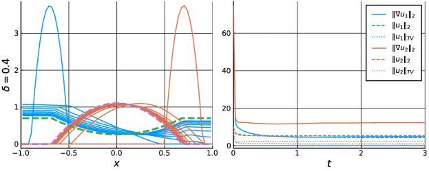
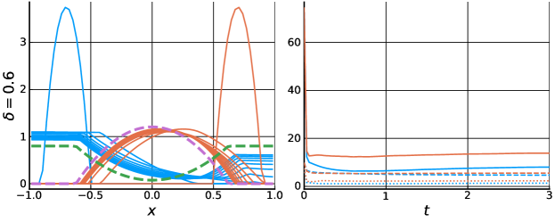
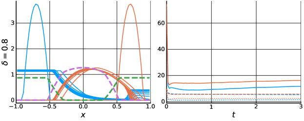
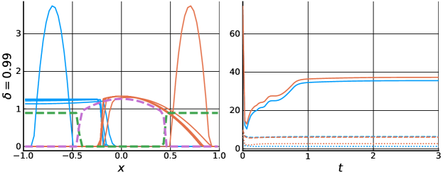
Figure 1: Time evolution with left and right initial conditions, $V_{1}=0$ and $V_{2}=2x^{2}$ and final time $T=3$, for various values of $\delta$ (Example 1). The left column shows ten equally spaced timepoints in $[0,T]$ in solid lines, and the stationary stated in dashed lines. The right column shows the temporal evolution of three norms.

In the right column of Fig. 1 we plot the time evolution of the spatial $L^{2}$ norms of $u_{i}$ and $\nabla u_{i}$, as well as the Total Variation (TV), all computed using the partition given by the spatial grid used in the finite-volume scheme. The key point to note is that the effect of increasing $\delta$ is noticed markedly by the semi-norm $\|\nabla u_{i}\|_{L^{2}}$, whereas the other two norms, $\|u_{i}\|_{L^{2}}$ and $\|u_{i}\|_{TV}$, remain mostly unchanged by $\delta$.

Example 2 (Uniform initial conditions).

Here we consider exactly the same set-up as in the previous example, except that now both components start with uniform initial conditions

$$u_{1,0}(x)=u_{2,0}(x)=1/|\Omega|.$$

Therefore, we expect the same stationary states (since for $\delta<1$, $E$ is strictly convex). We show the results of this example in Fig. 2. Because of the symmetry in the initial conditions, in this case the convergence to the steady state is much faster, as there is no mass that has to “cross” through the vacuum region as the latter is formed.

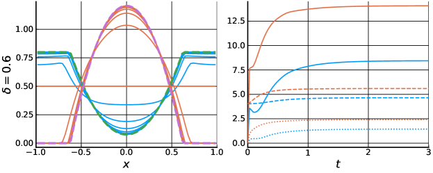
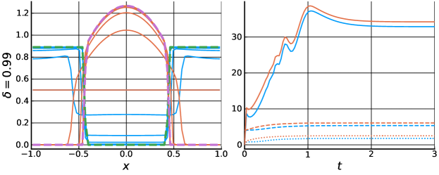
Figure 2: Time evolution with uniform initial conditions, $V_{1}=0$ and $V_{2}=2x^{2}$ and final time $T=3$, for various values of $\delta$ (Example 2). The left column shows ten equally spaced timepoints in $[0,T]$ in solid lines, and the stationary stated in dashed lines. The right column shows the temporal evolution of three norms.

Example 3 (Stronger external potentials).

We now consider the left and right initial conditions as in Example 1 while changing the external potentials to $V_{1}(x)=x^{2}/2$ and $V_{2}(x)=50x^{2}$. For this choice, we have that

$$\delta_{\max}(T)=0.00126,\quad\delta_{\max}(\Delta t)=0.480,$$

that is, a ten-fold reduction in $\delta_{\max}(T)$ with respect to Example 1 but a barely noticeable change in $\delta_{\max}(\Delta t)$ (as expected given that $\delta_{\max}$ is independent of $L_{i}$ in the small time limit). The stronger confinement potential in the second species leads to a vacuum region in the first species for smaller values of $\delta$ than in the previous examples, and the associated slower convergence (see Figure 3).

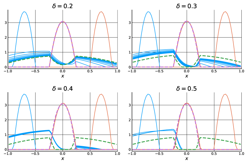
Figure 3: Time evolution with uniform initial conditions, $V_{1}(x)=x^{2}/2$ and $V_{2}(x)=50x^{2}$ and final time $T=3$, for various values of $\delta$ (Example 3). There are ten equally spaced timepoints in $[0,T]$ in solid lines, and stationary stated in dashed lines.

Example 4 (Evolution of norms in time and space as a function of $\delta$).

In this final example, we look at the evolution of the norms in $\delta$ instead of time. To this end, we consider the following integrated-in-time norms

$$\|u\|_{2,T} =\left\{\sum_{t_{k}=0}^{T}\left[\|u_{1}(t_{k},\cdot)\|_{L^{2}}^{2}+\|u_{2}(t_{k},\cdot)\|_{L^{2}}^{2}\right]\right\}^{1/2},$$

$$\|\nabla u\|_{2,T} =\left\{\sum_{t_{k}=0}^{T}\left[\|\nabla u_{1}(t_{k},\cdot)\|_{L^{2}}^{2}+\|\nabla u_{2}(t_{k},\cdot)\|_{L^{2}}^{2}\right]\right\}^{1/2},$$

$$\|u\|_{TV,T} =\left\{\sum_{t_{k}=0}^{T}\left[\|u_{1}(t_{k},\cdot)\|_{TV}+\|u_{2}(t_{k},\cdot)\|_{TV}\right]\right\}^{1/2}.$$

We use uniform initial conditions, a final time $T=5$, and values for $\delta=0,0.1,\dots,0.9,0.95,0.99$. We show the evolution of the three norms in Fig. 4 for two cases: first, for the potentials used in Examples 1 and 2, namely $V_{1}=0$ and $V_{2}=2x^{2}$; and second, for $V_{1}=x^{2}/2$ and $V_{2}=50x^{2}$. In the latter, the combination of external potentials makes the interface between the two components sharper (since the second component has a very strong confining potential, but also the first component now wants to concentrate around the origin). This fact is clearly visible in the trend of $\|\nabla u\|_{2,T}$ for increasing $\delta$. In contrast, the TV norm remains unchanged. As mentioned in the introduction, this observation indicates that a smallness assumption on $\delta$ is necessary in order to keep to the functional framework of $L^{2}(0,T;H^{1}(\Omega))$ for the analysis. The plot also illustrates that there is hope for a more general existence theory for solutions belonging to the space $BV$ when $\delta$ is close to $1$.

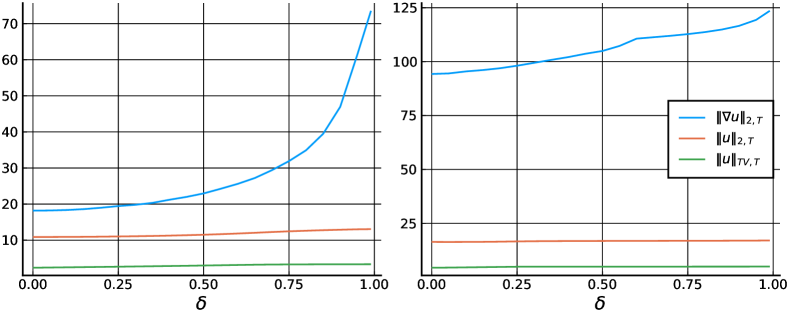
Figure 4: Norms (rescaled by $T|\Omega|$) in time and space as a function of $\delta$ with uniform initial conditions and final time $T=3$. (Left) $V_{1}=0$ and $V_{2}=2x^{2}$. (Right) $V_{1}=x^{2}/2$ and $V_{2}=50x^{2}$.

3 Regularised frozen system

We introduce below the regularised system with frozen cross-diffusion. Let $\bar{z}=(\bar{z}_{i})_{i=1}^{M}\in(C^{\infty}(\bar{Q}_{T}))^{M}$ be a given vector function. Throughout this section, we denote by $z=(z_{i})_{i=1}^{M}$ the solution of the regularised frozen system

$$\left\{\begin{aligned} &\partial_{t}z_{i}=\operatorname{div}[z_{i}(\nabla z_{i}+\nabla L_{i}(t,x,z_{i})+\delta F_{i}(t,x,\bar{z},\nabla\bar{z}))+\varepsilon\nabla z_{i}]\qquad&&\text{in }Q_{T},\\ &0=\nu\cdot[z_{i}(\nabla z_{i}+\nabla L_{i}(t,x,z_{i})+\delta F_{i}(t,x,\bar{z},\nabla\bar{z}))+\varepsilon\nabla z_{i}]\qquad&&\text{on }\Sigma_{T},\\ &z_{i}(0,\cdot)=z_{i,0}\qquad&&\text{on }\Omega.\end{aligned}\right.$$ (25)

Remark 3.1.

The constant $\varepsilon>0$ and the vector of non-negative functions $z_{0}=(z_{i,0})_{i=1}^{M}\in(C^{\infty}_{c}(\Omega))^{M}$ do not change throughout the present section and Section 4. The initial functions $z_{i,0}$ are chosen such that $\int_{\Omega}z_{i,0}\,\mathrm{d}x=\int_{\Omega}u_{i,0}\,\mathrm{d}x$ for $i\in\{1,\dots,M\}$.

In the next subsection we introduce the definition of weak solution to the above regularised frozen system, and show the mass conservation and non-negativity for such weak solutions. We then prove the existence of these solutions, and deduce from their regularity that they satisfy the system of equations in the classical sense. Then we prove some Sobolev estimates independent of $\varepsilon$, and conclude with a uniqueness result.

In what follows, we will sometimes use the shorthand $\bar{F}_{i}$ to refer to the function

$$\bar{F}_{i}(t,x):=F_{i}(t,x,\bar{z}(t,x),\nabla\bar{z}(t,x))\qquad\forall(t,x)\in\bar{Q}_{T}.$$ (26)

Remark 3.2.

In view of the condition that $\{G^{0}_{i}\}_{i=1}^{M}$ and $\{G^{1}_{ij}\}_{i,j=1}^{M}$ in (10) be $C^{2}$-regular and uniformly bounded with respect to all arguments (see Subsection 1.2), for each $\bar{z}=(\bar{z}_{i})_{i=1}^{M}\in(C^{\infty}(\bar{Q}_{T}))^{M}$ fixed, there exists a positive constant $\Lambda_{\bar{z}}$, where

$$\Lambda_{\bar{z}}=\Lambda_{\bar{z}}\left(\max_{1\leq i\leq M}\|\bar{z}_{i}\|_{C^{2}(\bar{Q}_{T})},\max_{1\leq i\leq M}\|F_{i}\|_{C^{2}(\bar{Q}_{T}\times\mathbb{R}^{M}\times\mathbb{R}^{Md})}\right),$$

such that, for all $(t,x)\in\bar{Q}_{T}$ and every $i\in\{1,\dots,M\}$,

$$|\bar{F}_{i}(t,x)|+\sum_{j=1}^{d}\left|\frac{\partial\bar{F}_{i}}{\partial x_{j}}(t,x)\right|+\left|\frac{\partial\bar{F}_{i}}{\partial t}(t,x)\right|+\sum_{j=1}^{d}\left|\frac{\partial^{2}\bar{F}_{i}}{\partial t\partial x_{j}}(t,x)\right|+\sum_{k=1}^{d}\sum_{j=1}^{d}\left|\frac{\partial^{2}\bar{F}_{i}}{\partial x_{k}\partial x_{j}}(t,x)\right|\leq\Lambda_{\bar{z}}.$$ (27)

Additionally, there exists a positive constant $\Lambda_{0}$ depending only on $(z_{i,0})_{i=1}^{M}$ such that

$$\|z_{i,0}\|_{C^{2}(\bar{\Omega})}\leq\Lambda_{0}.$$ (28)

3.1 Definition and existence of regularised solutions

In accordance with the definition of weak solution given in [49, Section 5.7], we provide the following notion of solution to the regularised frozen problem.

Definition 3.3 (Weak solution for regularised frozen system).

We say that $z\in(C^{2,1}(\bar{Q}_{T}))^{M}$ solves the weak form of (25) if, for any test function $\phi\in C^{1}(\bar{Q}_{T})$, for $i\in\{1,\dots,M\}$, for $t\in[0,T]$,

$$\int_{\Omega}z_{i}(t,x)\phi(t,x)\,\mathrm{d}x -\int_{\Omega}z_{i,0}(x)\phi(0,x)\,\mathrm{d}x-\int_{0}^{t}\int_{\Omega}z_{i}\partial_{t}\phi\,\mathrm{d}x\,\mathrm{d}t$$ (29)

$$+\int_{0}^{t}\int_{\Omega}\big{[}z_{i}(\nabla z_{i}+\nabla L_{i}(t,x,z_{i})+\delta F_{i}(t,x,\bar{z},\nabla\bar{z}))+\varepsilon\nabla z_{i}\big{]}\cdot\nabla\phi\,\mathrm{d}x\,\mathrm{d}t=0.$$

Correspondingly, we define $S_{\varepsilon}:\bar{z}\to z$ to be the solution operator, whose image is the weak solution of (25).

Remark 3.4.

Note that the following compatibility condition has been implicitly imposed in the previous weak formulation,

$$0=\nu\cdot\big{[}z_{i,0}(\nabla z_{i,0}+\nabla L_{i}(0,x,z_{i,0})+\delta F_{i}(0,x,\bar{z}(0,x),\nabla\bar{z}(0,x)))+\varepsilon\nabla z_{i,0}\big{]}\qquad\text{on }\partial\Omega,$$ (30)

which is manifestly satisfied for all choices of $\bar{z}\in(C^{\infty}(\bar{Q}_{T}))^{M}$, as the fixed initial data $z_{i,0}$ is identically zero on the boundary $\partial\Omega$ due to its compact support (see Remark 3.1).

Lemma 3.5 (Mass conservation for regularised frozen system).

Suppose there exists a weak solution $z$ of the problem (25) in the sense of Definition 3.3. Then, for $i\in\{1,\dots,M\}$,

$$\int_{\Omega}z_{i}(t,x)\,\mathrm{d}x=\int_{\Omega}z_{i,0}(x)\,\mathrm{d}x\qquad\forall t\in[0,T].$$

Proof.

The assertion is immediate from using the test function $\phi=1$ in Definition 3.3. ∎

Lemma 3.6 (Sign preservation for regularised frozen system).

Suppose there exists a weak solution $z$ of the problem (25) in the sense of Definition 3.3. Then, for $i\in\{1,\dots,M\}$,

$$z_{i}(t,x)\geq 0\qquad\text{for a.e. }(t,x)\in\bar{Q}_{T}.$$

Proof.

Define the function $\theta(t,x):=[z_{i}(t,x)]_{-}$ to be the negative part of the weak solution in question. Noting that $\theta=-z_{i}\mathds{1}_{z_{i}\leq 0}$, we observe that this function is non-negative and supported in the set $\{(t,x)\in\bar{Q}_{T}:z_{i}(t,x)\leq 0\}$. Moreover, we find that

$$\nabla\theta=-\nabla z_{i}\mathds{1}_{z_{i}\leq 0},\qquad\partial_{t}\theta=-\partial_{t}z_{i}\mathds{1}_{z_{i}\leq 0}$$

in the sense of distributions. It follows that $\theta\in L^{2}(0,T;H^{1}(\Omega))\cap L^{\infty}(0,T;L^{1}(\Omega))$ and $\partial_{t}\theta\in X^{\prime}\cap L^{2}(0,T;(H^{1}(\Omega))^{\prime})$. Using standard density arguments in Sobolev spaces, we may test against $\theta$ in the weak formulation of Definition 3.3. In turn, we obtain, for a.e. $t\in(0,T)$,

$$\frac{d}{dt}\int_{\Omega}\frac{1}{2}\theta^{2}(t,x)\,\mathrm{d}x+\int_{\Omega}\big{(}\theta|\nabla\theta|^{2}+\theta\nabla\theta\cdot\nabla L_{i}(t,x,z_{i})+\delta\theta\nabla\theta\cdot F_{i}(t,x,\bar{z},\nabla\bar{z})+\varepsilon|\nabla\theta|^{2}\big{)}\,\mathrm{d}x=0.$$ (31)

Given the form of the terms $\{L_{i}\}_{i=1}^{M}$ from (13), we have

$$\bigg{|}\int_{\Omega}\theta\nabla\theta\cdot\nabla L_{i}(t,x,z_{i})\,\mathrm{d}x\bigg{|}\leq\big{(}\|\nabla V_{i}(t,\cdot)\|_{L^{\infty}(\Omega)}+\|\nabla W_{i}*z_{i}(t,\cdot)\|_{L^{\infty}(\Omega)}\big{)}\int_{\Omega}\theta|\nabla\theta|\,\mathrm{d}x,$$

and

$$\|\nabla W_{i}*z_{i}(t,\cdot)\|_{L^{\infty}(\Omega)}\leq\|\nabla W_{i}\|_{L^{\infty}(\mathbb{R}^{d})}\|z_{i}(t,\cdot)\|_{L^{1}(\Omega)}\qquad\text{a.e.~{}}t\in(0,T).$$

It therefore follows, using the fact that $z_{i}\in L^{\infty}(0,T;L^{1}(\Omega))$ since $z_{i}\in C^{2,1}(\bar{Q}_{T})$ as per Definition 3.3, that

$$\bigg{|}\int_{\Omega}\theta\nabla\theta\cdot\nabla L_{i}(t,x,z_{i})\,\mathrm{d}x\bigg{|}\leq C_{L}\big{(}1+\|z_{i}\|_{L^{\infty}(0,T;L^{1}(\Omega))}\big{)}\int_{\Omega}\theta|\nabla\theta|\,\mathrm{d}x\qquad\text{a.e.~{}}t\in(0,T).$$

Meanwhile, using the boundedness of $\bar{z}$ and that of $F$ in $C^{2}$ to control $F_{i}(t,x,\bar{z},\nabla\bar{z})$ from (27) (see Remark 3.2), we obtain

$$\bigg{|}\int_{\Omega}\delta\theta\nabla\theta\cdot F_{i}(t,x,\bar{z},\nabla\bar{z})\,\mathrm{d}x\bigg{|}\leq|\delta|\Lambda_{\bar{z}}\int_{\Omega}\theta|\nabla\theta|\,\mathrm{d}x\qquad\text{a.e.~{}}t\in(0,T).$$

Integrating (31) with respect to the time variable, and using the previous estimates, we find

$$\int_{\Omega}\frac{1}{2}\theta^{2}(t,x)\,\mathrm{d}x+\int_{0}^{t}\int_{\Omega}\theta|\nabla\theta|^{2}\,\mathrm{d}x\,\mathrm{d}\tau+\varepsilon\int_{0}^{t}\int_{\Omega}|\nabla\theta|^{2}\,\mathrm{d}x\,\mathrm{d}\tau\leq \Lambda\int_{0}^{t}\int_{\Omega}\theta|\nabla\theta|\,\mathrm{d}x,$$

where the positive constant

$$\Lambda:=|\delta|\Lambda_{\bar{z}}+C_{L}\big{(}1+\|z_{i}\|_{L^{\infty}(0,T;L^{1}(\Omega))}\big{)}$$

is independent of time. An application of the Cauchy–Young inequality gives

$$\int_{\Omega}\frac{1}{2}\theta^{2}(t,x)\,\mathrm{d}x+\int_{0}^{t}\int_{\Omega}\theta|\nabla\theta|^{2}\,\mathrm{d}x\,\mathrm{d}\tau+\frac{\varepsilon}{2}\int_{0}^{t} \int_{\Omega}|\nabla\theta|^{2}\,\mathrm{d}x\,\mathrm{d}\tau\leq\frac{\Lambda^{2}}{\varepsilon}\int_{0}^{t}\int_{\Omega}\frac{1}{2}\theta^{2}\,\mathrm{d}x\,\mathrm{d}\tau.$$

Dropping the last two terms in the left-hand side of the inequality above, Grönwall’s Lemma yields

$$\int_{\Omega}\theta^{2}(t,x)\,\mathrm{d}x\leq\bigg{(}\int_{\Omega}\theta^{2}(0,x)\,\mathrm{d}x\bigg{)}e^{\frac{\Lambda^{2}}{\varepsilon}t}=0\qquad\text{for a.e. }t\in(0,T),$$

where the final equality follows from the non-negativity of the initial data $z_{i,0}$ (Remark 3.1). The result follows. ∎

Remark 3.7.

It is a priori not clear how to prove such a sign preservation result for the original system (12) directly from Definition 1.3, due to the presence of cross-terms of the form $\int_{\Omega}\nabla u_{j}(t,x)[u_{i}(t,x)]_{-}\,\mathrm{d}x$ with $i\neq j$. The non-negativity of the solution of the original system (12) will therefore be deduced via a limiting procedure from the non-negativity of the regularised solutions of (25).

In what follows, we apply the classical theory of Ladyzhenskaya, Solonnikov, and Uraltseva [49, Chap. 5, Sec. 7, Thm. 7.4] to deduce the existence and uniqueness of classical solutions to the regularised system (25). The proof is given in Appendix A.1.

Lemma 3.8 (Existence and uniqueness of regularised solutions).

There exists a unique $z=(z_{i})_{i=1}^{M}\in C^{2,1}(\bar{Q}_{T})$ solving (25) as a pointwise equality between continuous functions. Moreover, for $i\in\{1,\dots,M\}$,

$$z_{i}(t,x)\geq 0\quad\text{for }(t,x)\in\bar{Q}_{T},\quad z_{i}(0,x)=z_{i,0}(x)\quad\text{for }x\in\bar{\Omega},\quad\int_{\Omega}z_{i}(t,x)\,\mathrm{d}x=\int_{\Omega}z_{i,0}(x)\,\mathrm{d}x\quad\text{for }t\in[0,T].$$

3.2 Uniform estimates

In this subsection, we derive the uniform estimates on the solutions of the regularised frozen system by testing the equation against the logarithm of the solution.

Lemma 3.9 (Energy estimates).

Let $z=(z_{i})_{i=1}^{M}\in(C^{2,1}(\bar{Q}_{T}))^{M}$ be the solution of (25) provided by Lemma 3.8. Then, for any $t\in[0,T]$, there holds the estimate

$$\int_{\Omega}z_{i}(t)(\log z_{i}(t))_{+}\,\mathrm{d}x+\frac{1}{2}\int_{0}^{t}\int_{\Omega}|\nabla z_{i}|^{2}\,\mathrm{d}x\,\mathrm{d}\tau+\varepsilon\int_{0}^{t}\int_{\Omega}\frac{|\nabla z_{i}|^{2}}{z_{i}}\,\mathrm{d}x\,\mathrm{d}\tau\\ \leq(e^{-1}|\Omega|+2|\Omega|TC_{L}^{2})+\int_{\Omega}z_{i,0}\log z_{i,0}\,\mathrm{d}x+2|\Omega|TC_{L}^{2}\left(\int_{\Omega}z_{i,0}\,\mathrm{d}x\right)^{2}+\int_{0}^{T}\int_{\Omega}\delta^{2}|\bar{F}_{i}|^{2}\,\mathrm{d}x\,\mathrm{d}\tau,$$ (32)

for $i\in\{1,\dots,M\}$, along with the Sobolev estimate

$$\sup_{t\in[0,T]}\int_{\Omega}z_{i}(t)(\log z_{i}(t))_{+}\,\mathrm{d}x+\|z_{i} \|_{L^{2}(0,T;H^{1}(\Omega))}^{2}$$ (33)

$$\leq C_{\Omega}\bigg{(}1+\|z_{i,0}\|_{L^{1}(\Omega)}^{2}+\int_{\Omega}z_{i,0}\log z_{i,0}\,\mathrm{d}x+\int_{0}^{T}\int_{\Omega}\delta^{2}|\bar{F}_{i}|^{2}\,\mathrm{d}x\,\mathrm{d}t\bigg{)},$$

for $i\in\{1,\dots,M\}$. The positive constant $C_{\Omega}=C_{\Omega}(\Omega,T,d)$, which is independent of $\varepsilon$ and $z_{0}=(z_{i,0})_{i=1}^{M}$, is given by

$$C_{\Omega}=2\cdot\max\left\{(1+C_{P}),\frac{T}{|\Omega|}+2|\Omega|(1+C_{P})\big{(}e^{-1}+2TC_{L}^{2}\big{)}\right\},$$ (34)

where $C_{P}=C_{P}(\Omega,d)$ is the Poincaré constant.

Proof.

Begin by assuming that $z_{i}$ is strictly positive in $Q_{T}$ and multiply (25) by $\log z_{i}$. By rewriting the time derivative, we get

$$\partial_{t}(z_{i}\log z_{i})-\partial_{t}z_{i}=(\log z_{i})\operatorname{div}[z_{i}(\nabla z_{i}+\nabla L_{i}(t,x,z_{i})+\delta\bar{F}_{i})+\varepsilon\nabla z_{i}]\qquad\forall(t,x)\in Q_{T}.$$

Integrating in space and time then yields, for any $t\in[0,T]$,

$$\int_{0}^{t}\frac{d}{d\tau}\bigg{(}\int_{\Omega}z_{i}(\tau)\log z_{i}(\tau )\,\mathrm{d}x\bigg{)}\,\mathrm{d}\tau-\int_{0}^{t}\frac{d}{d\tau}\bigg{(}\int_{\Omega}z_{i}(\tau)\,\mathrm{d}x\bigg{)}\,\mathrm{d}\tau=$$ (35)

$$-\int_{0}^{t}\int_{\Omega}\left[\nabla z_{i}\cdot(\nabla z_{i}+\nabla L_{i}(t,x,z_{i})+\delta\bar{F}_{i})+\varepsilon\frac{|\nabla z_{i}|^{2}}{z_{i}}\right]\,\mathrm{d}x\,\mathrm{d}\tau,$$

where the no-flux boundary condition makes the boundary term vanish.

When $z_{i}$ is merely non-negative, we multiply by $\log(\beta+z_{i})$ for some $\beta>0$ and get

$$\partial_{t}(z_{i}\log(\beta+z_{i}))-(\partial_{t}z_{i})\frac{z_{i}}{\beta+z_{i}}=(\log(\beta+z_{i}))\operatorname{div}[z_{i}(\nabla z_{i}+\nabla L_{i}(t,x,z_{i})+\delta\bar{F}_{i})+\varepsilon\nabla z_{i}],\qquad\forall(t,x)\in Q_{T}.$$

Integrating in time and space, and using that $|\partial_{t}z_{i}|$ is integrable on $Q_{T}$ since $z_{i}$ is $C^{2,1}(\bar{Q}_{T})$, the Dominated Convergence Theorem implies

$$\lim_{\beta\to 0}\int_{0}^{t}\int_{\Omega}(\partial_{t}z_{i})\frac{z_{i}}{\beta+z_{i}}\,\mathrm{d}x\,\mathrm{d}\tau=\int_{0}^{t}\int_{\Omega}(\partial_{t}z_{i})\,\mathrm{d}x\,\mathrm{d}\tau.$$

All other terms may be treated similarly with the exception of the Fisher information, where one obtains

$$\lim_{\beta\to 0}\int_{0}^{t}\int_{\Omega}\frac{|\nabla z_{i}|^{2}}{\beta+z_{i}}\,\mathrm{d}x\,\mathrm{d}\tau=\int_{0}^{t}\int_{\Omega}\frac{|\nabla z_{i}|^{2}}{z_{i}}\,\mathrm{d}x\,\mathrm{d}\tau,$$

by the Monotone Convergence Theorem, since the sequence of integrands $\left\{|\nabla z_{i}|^{2}/(\beta+z_{i})\right\}_{\beta>0}$ is pointwise increasing as $\beta\to 0$ and non-negative by virtue of Lemma 3.8. In turn, we recover (35).

Recall from Lemma 3.8 that $\int_{\Omega}z_{i}(\tau)\,\mathrm{d}x$ is constant. Equation (35) therefore simplifies to

$$\int_{\Omega}z_{i}(t)\log z_{i}(t)\,\mathrm{d}x=\int_{\Omega}z_{i,0}\log z_{i,0}\,\mathrm{d}x-\delta\int_{0}^{t}\int_{\Omega}\nabla z_{i}\cdot\bar{F}_{i}\,\mathrm{d}x\,\mathrm{d}\tau -\int_{0}^{t}\int_{\Omega}|\nabla z_{i}|^{2}\,\mathrm{d}x\,\mathrm{d}\tau$$ (36)

$$-\int_{0}^{t}\int_{\Omega}\nabla z_{i}\cdot\nabla L_{i}(t,x,z_{i})\,\mathrm{d}x\,\mathrm{d}\tau -\varepsilon\int_{0}^{t}\int_{\Omega}\frac{|\nabla z_{i}|^{2}}{z_{i}}\,\mathrm{d}x\,\mathrm{d}\tau,$$

for any $t\in[0,T]$. Observe also that $z\log z=z\log z\mathds{1}_{\{z\geq 1\}}+z\log z\mathds{1}_{\{0\leq z<1\}}$, $\forall z\in[0,\infty),$ and, since $x\mapsto x\log x$ is non-positive over the interval $[0,1]$ and achieves its minimum (with value $-e^{-1}$) at the point $x=e^{-1}$, it follows that

$$z\log z\geq z\log z\mathds{1}_{\{z\geq 1\}}-e^{-1}\qquad\forall z\in[0,\infty).$$ (37)

Also, using (13), (14), and an application of the triangle inequality followed by Hölder’s inequality yields

$$\begin{aligned} \bigg{|}\int_{0}^{t}\int_{\Omega}\nabla z_{i}\cdot\nabla L_{i}(t,x,z_{i})\,\mathrm{d}x\,\mathrm{d}\tau\bigg{|}&\leq\|\nabla V_{i}\|_{L^{2}(Q_{T})}\|\nabla z_{i}\|_{L^{2}(Q_{T})}\\ &\qquad+\|\nabla z_{i}\|_{L^{2}(Q_{T})}\bigg{(}\int_{0}^{t}\int_{\Omega}|\nabla W_{i}*z_{i}(\tau,\cdot)(x)|^{2}\,\mathrm{d}x\,\mathrm{d}\tau\bigg{)}^{\frac{1}{2}}\\ &\leq(|\Omega|T)^{\frac{1}{2}}C_{L}\left(1+\int_{\Omega}z_{i,0}(y)\,\mathrm{d}y\right)\|\nabla z_{i}\|_{L^{2}(Q_{T})},\end{aligned}$$ (38)

where we bounded the convolution term as follows

$$\int_{0}^{t}\int_{\Omega}|\nabla W_{i}*z_{i}(\tau,\cdot)(x)|^{2}\,\mathrm{d}x\,\mathrm{d}\tau =\int_{0}^{t}\int_{\Omega}\bigg{|}\int_{\Omega}\nabla W_{i}(x-y)z_{i}(\tau,y)\,\mathrm{d}y\bigg{|}^{2}\,\mathrm{d}x\,\mathrm{d}\tau$$ (39)

$$\leq C_{L}^{2}\int_{0}^{t}\int_{\Omega}\bigg{(}\int_{\Omega}z_{i}(\tau,y)\,\mathrm{d}y\bigg{)}^{2}\,\mathrm{d}x\,\mathrm{d}\tau=C_{L}^{2}|\Omega|T\left(\int_{\Omega}z_{i,0}(y)\,\mathrm{d}y\right)^{2},$$

where we used the boundedness of $\{\nabla W_{i}\}_{i=1}^{M}$ inherited from (14), the non-negativity of $z_{i}$ due to Lemma 3.6, and the fact that $x\mapsto x^{2}$ is increasing on $[0,\infty)$ to obtain the inequality, and the mass conservation from Lemma 3.5 to obtain the final equality. Using estimates (37) and (38), along with an application of the weighted Cauchy–Young inequality to the terms on the right-hand side of (38) and to $\int_{0}^{t}\int_{\Omega}\nabla z_{i}\cdot\bar{F}_{i}\,\mathrm{d}x\,\mathrm{d}t$, we deduce the estimate (32) from (36).

The Poincaré–Wirtinger inequality

$$\int_{\Omega}\left(z_{i}-\frac{1}{|\Omega|}\int_{\Omega}z_{i}\,\mathrm{d}x\right)^{2}\,\mathrm{d}x\leq C_{P}\int_{\Omega}|\nabla z_{i}|^{2}\,\mathrm{d}x,$$

where $C_{P}=C_{P}(\Omega,d)$ is the Poincaré constant, implies

$$C_{P}\int_{\Omega}|\nabla z_{i}|^{2}\,\mathrm{d}x \geq\int_{\Omega}\left(z_{i}-\frac{1}{|\Omega|}\int_{\Omega}z_{i}\,\mathrm{d}x\right)^{2}\,\mathrm{d}x$$

$$=\int_{\Omega}\left[z_{i}^{2}-\frac{2}{|\Omega|}z_{i}\int_{\Omega}z_{i}\,\mathrm{d}x+\frac{1}{|\Omega|^{2}}\left(\int_{\Omega}z_{i}\,\mathrm{d}x\right)^{2}\right]\,\mathrm{d}x=\int_{\Omega}z_{i}^{2}\,\mathrm{d}x-\frac{1}{|\Omega|}\left(\int_{\Omega}z_{i,0}\,\mathrm{d}x\right)^{2},$$

where we used the conservation of mass in the final equality. Substituting back into (32), we get

$$\int_{0}^{T}\int_{\Omega}\frac{1}{2}z_{i}^{2}\,\mathrm{d}x\,\mathrm{d}t\leq\frac{T}{2|\Omega|}\left(\int_{\Omega}z_{i,0}\,\mathrm{d}x\right)^{2}+C_{P}(e^{-1}|\Omega|+2|\Omega|TC_{L}^{2})+C_{P}\int_{\Omega}z_{i,0}\log z_{i,0}\,\mathrm{d}x\\ +2C_{P}|\Omega|TC_{L}^{2}\left(\int_{\Omega}z_{i,0}\,\mathrm{d}x\right)^{2}+C_{P}\int_{0}^{T}\int_{\Omega}\delta^{2}|\bar{F}_{i}|^{2}\,\mathrm{d}x\,\mathrm{d}\tau.$$

Combining the above with (32), we obtain

$$\int_{0}^{T}\int_{\Omega}\frac{1}{2}(z_{i}^{2}+|\nabla z_{i}|^{2})\,\mathrm{d}x\,\mathrm{d}t\leq \left(\frac{T}{2|\Omega|}+2(1+C_{P})|\Omega|TC_{L}^{2}\right)\left(\int_{\Omega}z_{i,0}\,\mathrm{d}x\right)^{2}$$

$$+(1+C_{P})(e^{-1}|\Omega|+2|\Omega|TC_{L}^{2})+(1+C_{P})\int_{\Omega}z_{i,0}\log z_{i,0}\,\mathrm{d}x$$

$$+(1+C_{P})\int_{0}^{T}\int_{\Omega}\delta^{2}|\bar{F}_{i}|^{2}\,\mathrm{d}x\,\mathrm{d}t,$$

from which we recover (33) with the appropriate constant $C_{\Omega}$ given by (34). ∎

Before proceeding to the next lemma, which covers the uniform estimate for the time derivative of the regularised solutions, we recall the interpolation result of Di Benedetto.

Proposition 3.10 (Proposition 3.2 of [35]).

Let $m,p\geq 1$ and assume that $\partial\Omega$ is piecewise smooth. There exists a constant $\gamma$ depending only on $d,m,p$ and the structure of $\partial\Omega$ such that, for any $v\in V^{m.p}$, where

$$V^{m.p}:=L^{\infty}(0,T;L^{m}(\Omega))\cap L^{p}(0,T;W^{1,p}(\Omega)),$$ (40)

we have

$$\left\|v\right\|_{L^{q}(Q_{T})}\leq\gamma\left(1+\frac{T}{|\Omega|^{\frac{d(p-m)+pm}{dm}}}\right)\left\|v\right\|_{V^{m.p}},\qquad\text{where }q=p\frac{d+m}{d}.$$ (41)

Lemma 3.11 (Time derivative estimate of the regularised solutions).

Recall the space $X$ introduced in Definition 1.2. There holds the uniform estimate in the dual space

$$\left\|\partial_{t}z_{i}\right\|_{X^{\prime}}\leq C_{X^{\prime}}\bigg{(}1+\|z_{i,0}\|_{L^{1}(\Omega)}^{2}+\int_{\Omega}z_{i,0}\log z_{i,0}\,\,\mathrm{d}x+\delta^{2}\left\|\bar{F}_{i}\right\|_{L^{2}(Q_{T})}^{2}\bigg{)},$$ (42)

where the positive constant $C_{X^{\prime}}=C_{X^{\prime}}(\Omega,T,d)$, which is independent of $\varepsilon$ and $z_{0}=(z_{i,0})_{i=1}^{M}$, is given by

$$C_{X^{\prime}}=2\gamma\left[\left(1+\frac{T}{|\Omega|^{\frac{d+2}{d}}}\right)+(|\Omega|T)^{\frac{d}{r}}\right]\left(2+3C_{\Omega}+2|\Omega|TC_{L}^{2}\right).$$ (43)

Proof.

Applying Proposition 3.10 with $v=z_{i}$, $m=1$, and $p=2$ yields

$$\left\|z_{i}\right\|_{L^{q}(Q_{T})}\leq\gamma\left(1+\frac{T}{|\Omega|^{\frac{d+2}{d}}}\right)\left\|z_{i}\right\|_{V^{1.2}},\quad q=2\frac{d+1}{d},$$ (44)

where the space $V^{1,2}$ is defined in (40). Notice that $q>2$ for all choices of dimension $d$.

Fix $\eta\in C^{\infty}(\bar{Q}_{T})$. Going back to (25), writing $\langle\partial_{t}z_{i},\eta\rangle=\int_{0}^{T}\int_{\Omega}\partial_{t}z_{i}\eta\,\mathrm{d}x\,\mathrm{d}t$, and using the divergence theorem in conjunction with the no-flux boundary condition, we find

$$|\langle\partial_{t}z_{i},\eta\rangle|=\bigg{|}\int_{0}^{T}\int_{\Omega}\nabla\eta\cdot[z_{i}(\nabla z_{i}+\nabla L_{i}(t,x,z_{i})+\delta\bar{F}_{i})+\varepsilon\nabla z_{i}]\,\mathrm{d}x\,\mathrm{d}t\bigg{|},$$ (45)

from which we obtain, using the triangle inequality,

$$|\langle\partial_{t}z_{i},\eta\rangle|\leq\int_{0}^{T}\int_{\Omega}|\nabla\eta|z_{i}|\nabla z_{i}+\nabla L_{i}(t,x,z_{i})+\delta\bar{F}_{i}|\,\mathrm{d}x\,\mathrm{d}t+\varepsilon\int_{0}^{T}\int_{\Omega}|\nabla\eta||\nabla z_{i}|\,\mathrm{d}x\,\mathrm{d}t.$$

Then, using Hölder’s inequality, we get

$$|\langle\partial_{t}z_{i},\eta\rangle|\leq\left\|z_{i}\right\|_{L^{q}(Q_{T})} \left\|\nabla z_{i}+\nabla L_{i}(\cdot,\cdot,z_{i})+\delta\bar{F}_{i}\right\|_{L^{2}(Q_{T})}\left\|\nabla\eta\right\|_{L^{r}(Q_{T})}+\varepsilon\left\|\nabla\eta\right\|_{L^{2}(Q_{T})}\left\|\nabla z_{i}\right\|_{L^{2}(Q_{T})},$$ (46)

where $r$ satisfies $\frac{1}{q}+\frac{1}{r}=\frac{1}{2},$ and $q$ is as given in (44). Hence $r=2(d+1)>2$ and, since $Q_{T}=(0,T)\times\Omega$ is a bounded domain, an application of the Hölder inequality shows that

$$\left\|\nabla\eta\right\|_{L^{2}(Q_{T})} =\bigg{(}\int_{0}^{T}\int_{\Omega}|\nabla\eta|^{2}\,\mathrm{d}x\,\mathrm{d}t\bigg{)}^{\frac{1}{2}}$$

$$\leq\bigg{(}\int_{0}^{T}\int_{\Omega}|\nabla\eta|^{2(d+1)}\,\mathrm{d}x\,\mathrm{d}t\bigg{)}^{\frac{1}{2(d+1)}}\bigg{(}\int_{0}^{T}\int_{\Omega}1\,\mathrm{d}x\,\mathrm{d}t\bigg{)}^{\frac{d}{2(d+1)}}=(|\Omega|T)^{\frac{d}{r}}\left\|\nabla\eta\right\|_{L^{r}(Q_{T})}.$$

Combining the above with (44) and (46) shows that, with $C_{\gamma}=C_{\gamma}(\Omega,T,d)$ a positive constant given by

$$C_{\gamma}=\gamma\left(1+\frac{T}{|\Omega|^{\frac{d+2}{d}}}\right)+(|\Omega|T)^{\frac{d}{r}},$$

which is independent of $\varepsilon\in(0,1)$ and $z_{0}=(z_{i,0})_{i=1}^{M}$, there holds

$$|\langle\partial_{t}z_{i},\eta\rangle|\leq C_{\gamma}\left\|\nabla\eta\right\|_{L^{r}(Q_{T})}\bigg{(} \left\|z_{i}\right\|_{L^{2}(0,T;H^{1}(\Omega))}$$

$$+\left\|z_{i}\right\|_{V^{1,2}}\big{(}\left\|z_{i}\right\|_{L^{2}(0,T;H^{1}(\Omega))}+\|\nabla L_{i}(\cdot,\cdot,z_{i})\|_{L^{2}(Q_{T})}+\delta\left\|\bar{F}_{i}\right\|_{L^{2}(Q_{T})}\big{)}\bigg{)},$$

for any $\eta\in C^{\infty}(\bar{Q}_{T})$, where we also used Minkowski’s inequality. Using the Cauchy–Young inequality on both of the terms inside the large brackets gives

$$|\langle\partial_{t}z_{i},\eta\rangle|\leq 2C_{\gamma}\bigg{(}1+\left\|z_{i}\right\|_{V^{1,2}}^{2} +\left\|z_{i}\right\|_{L^{2}(0,T;H^{1}(\Omega))}^{2}+\|\nabla L_{i}(\cdot,\cdot,z_{i})\|_{L^{2}(Q_{T})}^{2}+\delta^{2}\left\|\bar{F}_{i}\right\|_{L^{2}(Q_{T})}^{2}\bigg{)}\left\|\nabla\eta\right\|_{L^{r}(Q_{T})},$$ (47)

for any $\eta\in C^{\infty}(\bar{Q}_{T})$. Observe then that

$$\|\nabla L_{i}(\cdot,\cdot,z_{i})\|_{L^{2}(Q_{T})}\leq\|\nabla V_{i}\|_{L^{2}(Q_{T})}+\bigg{(}\int_{0}^{T}\int_{\Omega}|\nabla W_{i}*z_{i}(t,\cdot)(x)|^{2}\,\mathrm{d}x\,\mathrm{d}t\bigg{)}^{\frac{1}{2}},$$

where we estimate the second term on the right-hand side in the same way as in (39). It follows that

$$\|\nabla L_{i}(\cdot,\cdot,z_{i})\|_{L^{2}(Q_{T})}\leq(|\Omega|T)^{\frac{1}{2}}C_{L}\left(1+\int_{\Omega}z_{i,0}\,\mathrm{d}x\right).$$ (48)

Note also that the mass conservation of Lemma 3.5 yields

$$\left\|z_{i}\right\|_{V^{1,2}}\leq\left\|z_{i,0}\right\|_{L^{1}(\Omega)}+\left\|z_{i}\right\|_{L^{2}(0,T;H^{1}(\Omega))}.$$

By combining the above with (47) along with (48), and with the estimate (33) of Lemma 3.9, we obtain

$$|\langle\partial_{t}z_{i},\eta\rangle|\leq C_{X^{\prime}}\bigg{(}1+\left\|z_{i,0}\right\|_{L^{1}(\Omega)}^{2}+\int_{\Omega}z_{i,0}\log z_{i,0}\,\mathrm{d}x+\delta^{2}\left\|\bar{F}_{i}\right\|_{L^{2}(Q_{T})}^{2}\bigg{)}\left\|\nabla\eta\right\|_{L^{r}(Q_{T})},$$

for any $\eta\in C^{\infty}(\bar{Q}_{T})$, with $C_{X^{\prime}}=2C_{\gamma}\big{(}2+3C_{\Omega}+2|\Omega|TC_{L}^{2}\big{)},$ i.e., as given in (43), which is independent of $\varepsilon$ and $z_{0}=(z_{i,0})_{i=1}^{M}$. Using the density of the smooth functions in the space $L^{r}(0,T;W^{1,r}(\Omega))$, we take the supremum over all test functions $\eta\in L^{r}(0,T;W^{1,r}(\Omega))$ in the previous estimate, and deduce the uniform estimate (42). ∎

We also make note of the following quantitative estimate on the second derivatives of the regularised solutions. The proof is contained in Appendix A.2.

Lemma 3.12 (Second derivative estimate).

For the regularised frozen system (25), there holds, for $i\in\{1,\dots,M\}$, the estimate

$$\|\Delta z_{i}\|_{L^{2}(Q_{T})}\leq C(\varepsilon,\delta,T,\Omega,C_{L},\|z_{i,0}\|_{C^{1}(\bar{\Omega})},\|\bar{F}_{i}\|_{L^{\infty}(0,T;W^{1,\infty}(\Omega))},\|\partial_{t}\bar{F}_{i}\|_{L^{1}(0,T;L^{2}(\Omega))}),$$ (49)

where the right-hand side is a positive quantity depending only on the parameters in its parentheses.

3.3 Uniqueness of weak solutions to the regularised frozen problem

The following result provides a correspondence between equivalent weak formulations of the regularised frozen problem (25). Note that the proof also holds for the weak formulation of the original problem, as mentioned in Remark 1.5.

Lemma 3.13 (Equivalence of weak formulations of (25)).

Let $z=(z_{i})_{i=1}^{M}\in\Xi$ and denote the flux by $\mathcal{F}_{i}:=z_{i}(\nabla z_{i}+\nabla L_{i}(t,x,z_{i})+\delta F_{i}(t,x,\bar{z},\nabla\bar{z}))+\varepsilon\nabla z_{i}$. The following formulations are equivalent:

1. for each $i\in\{1,\dots,M\}$, for every $\eta\in C^{1}(\bar{\Omega})$, for a.e. $t\in[0,T]$,

   $$\langle\partial_{t}z_{i}(t,\cdot),\eta\rangle_{\Omega}+\int_{\Omega}\mathcal{F}_{i}\cdot\nabla\eta\,\mathrm{d}x=0,$$ (50)

   where $\langle\cdot,\cdot\rangle_{\Omega}$ is the duality product of $W^{1,r}(\Omega)$;

2. for each $i\in\{1,\dots,M\}$, for every $\phi\in C^{1}(\bar{Q}_{T})$,

   $$\langle\partial_{t}z_{i},\phi\rangle_{X^{\prime}\times X}+\int_{Q_{T}}\mathcal{F}_{i}\cdot\nabla\phi\,\mathrm{d}x\,\mathrm{d}t=0;$$ (51)

3. for each $i\in\{1,\dots,M\}$, for every $\phi\in C^{1}(\bar{Q}_{T})$ with $\phi(0,\cdot)=\phi(T,\cdot)=0$ on $\bar{\Omega}$,

   $$\int_{Q_{T}}\big{(}-z_{i}\partial_{t}\phi+\mathcal{F}_{i}\cdot\nabla\phi\big{)}\,\mathrm{d}x\,\mathrm{d}t=0.$$ (52)

Proof.

Before proving the lemma, we recall some useful facts. Firstly, as already noted in Remark 1.5, the definition of the space $\Xi$ implies $z_{i}\in W^{1,r^{\prime}}(0,T;(W^{1,r}(\Omega))^{\prime})$. This implies, by [39, Theorem 2 of Section 5.9.2], that $z_{i}\in C([0,T];(W^{1,r}(\Omega))^{\prime})$ and

$$z_{i}(t_{2},\cdot)-z_{i}(t_{1},\cdot)=\int_{t_{1}}^{t_{2}}\partial_{t}z_{i}(t,\cdot)\,\mathrm{d}t\quad\text{in }(W^{1,r}(\Omega))^{\prime}\quad\forall 0\leq t_{1}<t_{2}\leq T,$$

and hence, given any $\eta\in C^{1}(\bar{\Omega})$, there holds

$$\int_{\Omega}z_{i}(t_{2},x)\eta(x)\,\mathrm{d}x-\int_{\Omega}z_{i}(t_{1},x)\eta(x)\,\mathrm{d}x=\int_{t_{1}}^{t_{2}}\langle\partial_{t}z_{i}(t,\cdot),\eta\rangle\,\mathrm{d}t\quad\forall 0\leq t_{1}<t_{2}\leq T,$$ (53)

where the order of Bochner integration and the duality product were interchanged, which is justified by [39, Appendix E.5, Theorem 8] and the summability

$$\int_{0}^{T}\|\partial_{t}z_{i}(t,\cdot)\|_{(W^{1,r}(\Omega))^{\prime}}\,\mathrm{d}t\leq T^{\frac{1}{r}}\|\partial_{t}z_{i}\|_{X^{\prime}}.$$ (54)

Recall also the definition of weak time derivative in terms of Bochner integration (cf. [39, Section 5.9.2]). That is, for $z_{i}\in L^{r^{\prime}}(0,T;(W^{1,r}(\Omega))^{\prime})$, the element $\partial_{t}z_{i}\in L^{r^{\prime}}(0,T;(W^{1,r^{\prime}}(\Omega)^{\prime})$ is such that

$$\int_{0}^{T}\theta^{\prime}(t)z_{i}(t,\cdot)\,\mathrm{d}t=-\int_{0}^{T}\theta(t)\partial_{t}z_{i}(t,\cdot)\,\mathrm{d}t\qquad\forall\theta\in C^{1}_{c}((0,T)),$$ (55)

where the equality holds in the sense of $(W^{1,r}(\Omega))^{\prime}$. We are now in a position to prove the lemma.

Step I [2.$\iff$1.]: Begin with the forward implication. Fix any $\eta\in C^{1}(\bar{\Omega})$ and subsequently choose $\phi(t,x):=\theta(t)\eta(x)$ where $\theta\in C^{1}([0,T])$ is arbitrarily chosen. Then, (51) and the identification (17) made in Remark 1.5 imply $\int_{0}^{t}\big{(}\langle\partial_{t}z_{i}(\tau,\cdot),\eta\rangle_{\Omega}+\int_{\Omega}\mathcal{F}_{i}\cdot\nabla\eta\,\mathrm{d}x\big{)}\theta(\tau)\,\mathrm{d}\tau=0$. We deduce (50), using the arbitrariness of $\theta$ and the Fundamental Lemma of Calculus of Variations.

The converse follows from the density in $C^{1}(\bar{Q}_{T})$ of the subalgebra $\{\theta(t)\eta(x):\theta\in C^{1}([0,T]),\eta\in C^{1}(\bar{\Omega})\}$, due to Nachbin’s version of the Weierstraß Approximation Theorem [55], using the continuity of $\partial_{t}z_{i}$ as an element of $X^{\prime}$ for the duality term (indeed, convergence in $C^{1}(\bar{Q}_{T})$ implies convergence in $X$) and the Dominated Convergence Theorem for the integral term.

Step II [2.$\iff$3.]: Testing (55) with $\eta\in C^{1}(\bar{\Omega})$, using the summability (54) to exchange the order of Bochner integration and the duality product in $W^{1,r}(\Omega)$, as well as the Tonelli–Fubini Theorem, we obtain

$$\int_{Q_{T}}z_{i}(t,x)\theta^{\prime}(t)\eta(x)\,\mathrm{d}x\,\mathrm{d}t=-\int_{0}^{T}\langle\partial_{t}z_{i}(t,\cdot),\theta(t)\eta(\cdot)\rangle_{\Omega}\,\mathrm{d}t\qquad\forall\theta\in C^{1}_{c}((0,T)),\forall\eta\in C^{1}(\bar{\Omega}).$$ (56)

Using the identification (17) from Remark 1.5, we recognise the right-hand side of the above as $\langle\partial_{t}z_{i},\theta\eta\rangle_{X^{\prime}\times X}$. Thus, from the above, we obtain the equivalence of (51) and (52) in the particular instance of test functions of the form $\phi(t,x)=\theta(t)\eta(x)$ with $\theta\in C^{1}_{c}((0,T))$ and $\eta\in C^{1}(\bar{\Omega})$. Note that this subset of functions is dense in $\{\phi\in C^{1}(\bar{Q}_{T}):\phi(0,\cdot)=\phi(T,\cdot)=0\text{ on }\bar{\Omega}\}$ endowed with the subspace topology of $C^{1}(\bar{Q}_{T})$. The result then follows from the continuity of $\partial_{t}z_{i}$ as an element of $X^{\prime}$ for the duality term, and the Dominated Convergence Theorem for all remaining terms. ∎

The next result is the focal point of this subsection, and is concerned with the uniqueness of solutions to the regularised frozen problem in the larger space $\Xi$.

Lemma 3.14 (Uniqueness for regularised frozen problem in $\Xi$).

There exists a unique $z=(z_{i})_{i=1}^{M}\in\Xi$ such that, for every $i\in\{1,\dots,M\}$, $\int_{\Omega}z_{i}(t,x)\,\mathrm{d}x=\int_{\Omega}z_{i,0}(x)\,\mathrm{d}x$, $z_{i}(0,\cdot)=z_{i,0}$ in $(W^{1,r}(\Omega))^{\prime}$ and, for every $\eta\in C^{1}(\bar{Q}_{T})$,

$$\langle\partial_{t}z_{i},\eta\rangle_{X^{\prime}\times X}+\int_{Q_{T}}\left[z_{i}(\nabla z_{i}+\nabla L_{i}(t,x,z_{i})+\delta F_{i}(t,x,\bar{z},\nabla\bar{z}))+\varepsilon\nabla z_{i}\right]\cdot\nabla\eta\,\mathrm{d}x\,\mathrm{d}t=0.$$ (57)

Proof.

Let $z$ and $z^{*}$ satisfy the hypotheses and let $w:=z_{i}-z_{i}^{*}$. Problem (57) is nonlinear, however we can formally derive a dual equation through integration by parts and properties of the convolution. Specifically, supposing that the convolution kernel $H$ is radially symmetric, and that the functions below are sufficiently integrable, we note the following property:

$$\int_{\Omega}f(x)(H*g)(x)\,\mathrm{d}x=\int_{\Omega\times\Omega}f(x)H(x-y)g(y)\,\mathrm{d}y\,\mathrm{d}x=\int_{\Omega}(H*f)(y)g(y)\,\mathrm{d}y,$$

which follows directly from the Tonelli–Fubini Theorem. In the sequel we use the notation $\bar{F}_{i}$ introduced in (26), and we drop the arguments of $\bar{F}_{i}$, $V_{i}$ and $W_{i}$. Define $\phi\in L^{2}(0,T;H^{2}(\Omega))\cap H^{1}(0,T;L^{2}(\Omega))$ as a strong solution of the following linear and strongly parabolic dual equation:

$$\partial_{t}\phi-(\varepsilon+a_{\kappa})\Delta\phi+(\nabla V_{i}+\delta\bar{F}_{i}+\nabla W_{i}*z_{i})\cdot\nabla\phi+\sum\nolimits_{k=1}^{d}(\partial_{x_{k}}W_{i})*(z_{i}^{*}\partial_{x_{k}}\phi) =-\xi \text{ in }Q_{T},$$ (58)

$$\nabla\phi\cdot\nu =0 \text{ on }\Sigma_{T},$$

$$\phi(0,\cdot) =0 \text{ on }\Omega,$$

where $\xi\in C_{c}^{\infty}(Q_{T})$ is arbitrary and $\{a_{\kappa}\}_{\kappa\in\mathbb{N}}$ is a monotone sequence of bounded functions that approximate $\frac{z_{i}+z_{i}^{*}}{2}$; in particular, we choose

$$a_{\kappa}:=\min\left\{\left(\frac{z_{i}+z_{i}^{*}}{2}\right),\kappa\right\}.$$

Note that $a_{\kappa}\geq 0$ belongs to $L^{\infty}(Q_{T})$ for every $\kappa\in\mathbb{N}$. Consider now the equation for the time-shifted function $\psi(t,x)=\phi(T-t,x)$:

$$\partial_{t}\psi+(\varepsilon+a_{\kappa})\Delta\psi-(\nabla V_{i}+\delta\bar{F}_{i}+\nabla W_{i}*z_{i})\cdot\nabla\psi-\sum\nolimits_{k=1}^{d}(\partial_{x_{k}}W_{i})*(z_{i}^{*}\partial_{x_{k}}\psi) =\xi \text{ in }Q_{T},$$ (59)

$$\nabla\psi\cdot\nu =0 \text{ on }\Sigma_{T},$$

$$\psi(T,\cdot) =0 \text{ on }\Omega,$$

and test against a bounded $C^{1}$ function $\theta:[0,T]\to[1,\infty)$ such that $\partial_{t}\theta\geq 1$. We have, for every $t\in[0,T]$,

$$\int_{t}^{T}\int_{\Omega}\partial_{t}\psi\,\theta\Delta\psi\,\mathrm{d}x\,\mathrm{d}\tau =-\int_{t}^{T}\int_{\Omega}\frac{\theta}{2}\partial_{t}\left(|\nabla\psi|^{2}\right)\,\mathrm{d}x\,\mathrm{d}\tau$$

$$=-\int_{\Omega}\frac{1}{2}\left(\theta(T)|\nabla\psi(T,x)|^{2}-\theta(t)|\nabla\psi(t,x)|^{2}\right)\,\mathrm{d}x+\int_{t}^{T}\int_{\Omega}|\nabla\psi|^{2}\partial_{t}\left(\frac{\theta}{2}\right)\,\mathrm{d}x\,\mathrm{d}\tau$$

$$\geq\int_{\Omega}\frac{1}{2}|\nabla\psi(t,x)|^{2}\,\mathrm{d}x+\int_{t}^{T}\int_{\Omega}\frac{1}{2}|\nabla\psi|^{2}\,\mathrm{d}x\,\mathrm{d}\tau,$$

where we used $\phi(0,\cdot)=\psi(T,\cdot)=0$ and the lower bound on $\theta$. On the other hand, we also have

$$\int_{t}^{T}\int_{\Omega}\partial_{t}\psi\,\theta\Delta\psi\,\mathrm{d}x\,\mathrm{d}\tau =\int_{t}^{T}\int_{\Omega}\theta\bigg{[}-(\varepsilon+a_{\kappa})|\Delta\psi|^{2}+(\nabla V_{i}+\delta\bar{F}_{i}+\nabla W_{i}*z_{i})\cdot\nabla\psi\Delta\psi$$ (60)

$$\qquad\qquad+\sum\nolimits_{k=1}^{d}(\partial_{x_{k}}W_{i})*(z_{i}^{*}\partial_{x_{k}}\psi)\Delta\psi+\xi\Delta\psi\bigg{]}\,\mathrm{d}x\,\mathrm{d}\tau.$$

Firstly, we estimate the drift terms: letting $\mathcal{G}:=\nabla V_{i}+\delta\bar{F}_{i}+\nabla W_{i}*z_{i}$,

$$\int_{t}^{T}\int_{\Omega}\theta\mathcal{G}\cdot\nabla\psi\,\Delta\psi\,\mathrm{d}x\,\mathrm{d}\tau =\int_{t}^{T}\int_{\Omega}\frac{\theta}{2}|\nabla\psi|^{2}\operatorname{div}\mathcal{G}\,\mathrm{d}x\,\mathrm{d}\tau-\int_{t}^{T}\int_{\Omega}\theta\sum\nolimits_{k,l}\partial_{x_{k}}\psi\,\partial_{x_{l}}\mathcal{G}_{k}\,\partial_{x_{l}}\psi\,\mathrm{d}x\,\mathrm{d}\tau$$

$$\leq\left(\frac{1}{2}+d^{2}\right)\|\theta\|_{L^{\infty}([0,T])}\|\nabla\mathcal{G}\|_{L^{\infty}(Q_{T})}\int_{Q_{T}}|\nabla\psi|^{2}\,\mathrm{d}x\,\mathrm{d}t,$$

where we used that $\mathcal{G}$ and its space derivative are bounded, since the nonlocal drift is bounded by $\|\nabla W_{i}*z_{i}\|_{L^{\infty}(Q_{T})}\leq\|W_{i}\|_{C^{1}(\mathbb{R}^{d})}\|z_{i,0}\|_{L^{1}(\Omega)}$. Secondly, we estimate the nonlocal term:

$$\bigg{|}\int_{t}^{T}\int_{\Omega}\theta\sum\nolimits_{k=1}^{d}(\partial_{x_{k}}W_{i})*(z_{i}^{*} \partial_{x_{k}}\psi)\Delta\psi\,\mathrm{d}x\,\mathrm{d}\tau\bigg{|}$$

$$=\bigg{|}\int_{t}^{T}\int_{\Omega}\theta\sum\nolimits_{k=1}^{d}(\nabla\partial_{x_{k}}W_{i})*(z_{i}^{*}\partial_{x_{k}}\psi)\cdot\nabla\psi\,\mathrm{d}x\,\mathrm{d}\tau\bigg{|}$$

$$\leq d\|\theta\|_{L^{\infty}([0,T])}\|W_{i}\|_{C^{2}(\mathbb{R}^{d})}\int_{t}^{T}\int_{\Omega}|\nabla\psi(\tau,x)|\bigg{(}\int_{\Omega}|z_{i}^{*}(\tau,y)\nabla\psi(\tau,y)|\,\mathrm{d}y\bigg{)}\,\mathrm{d}x\,\mathrm{d}\tau$$

$$\leq d|\Omega|^{\frac{1}{2}}\|\theta\|_{L^{\infty}([0,T])}\|W_{i}\|_{C^{2}(\mathbb{R}^{d})}\int_{t}^{T}\|z^{*}_{i}(\tau,\cdot)\|_{L^{2}(\Omega)}\|\nabla\psi(\tau,\cdot)\|^{2}_{L^{2}(\Omega)}\,\mathrm{d}\tau,$$

where we integrated by parts to obtain the first equality and used the Hölder inequality to obtain both the second and the final lines. By integrating the term in (60) involving $\xi\Delta\psi$ by parts, and then using the Cauchy–Schwarz integral inequality followed by the Young inequality, we have obtained

$$\frac{1}{2}\| \nabla\psi(t,\cdot)\|_{L^{2}(\Omega)}^{2}+\int_{t}^{T}\int_{\Omega}\big{(}\frac{1}{2}|\nabla\psi|^{2}+(\varepsilon+a_{\kappa})|\Delta\psi|^{2}\big{)}\,\mathrm{d}x\,\mathrm{d}\tau$$ (61)

$$\leq \frac{1}{2}\|\nabla\xi\|_{L^{2}(Q_{T})}^{2}+C(d,|\Omega|,\|\theta\|_{L^{\infty}},\|\nabla\mathcal{G}\|_{L^{\infty}},\|W_{i}\|_{C^{2}})\int_{t}^{T}(1+\|z^{*}_{i}(\tau,\cdot)\|_{L^{2}(\Omega)})\frac{1}{2}\|\nabla\psi(\tau,\cdot)\|^{2}_{L^{2}(\Omega)}\,\mathrm{d}x\,\mathrm{d}\tau.$$

From the above we deduce, by first estimating the integrand in the right-hand side by its supremum over $[\tau,T]$ and then bounding the left-hand side similarly, that for every $t\in[0,T]$ there holds

$$\frac{1}{2}\sup_{\tau\in[t,T]}\|\nabla\psi(\tau,\cdot)\|_{L^{2}(\Omega)}^{2}\leq \frac{1}{2}\|\nabla\xi\|_{L^{2}(Q_{T})}^{2}+C\int_{t}^{T}(1+\|z^{*}_{i}(\tau,\cdot)\|_{L^{2}(\Omega)})\frac{1}{2}\sup_{y\in[\tau,T]}\|\nabla\psi(y,\cdot)\|^{2}_{L^{2}(\Omega)}\,\mathrm{d}x\,\mathrm{d}\tau.$$

where we used the shorthand $C$ to denote the quantity with the same name appearing on the right-hand side of (61). Applying the Grönwall Lemma (starting from the initial point $t=T$, where $\psi(T,\cdot)=\phi(0,\cdot)=0$) to this latter inequality yields

$$\sup_{t\in[0,T]}\|\nabla\psi(t,\cdot)\|_{L^{2}(\Omega)}^{2}\leq\|\nabla\xi\|_{L^{2}(Q_{T})}^{2}\exp\left(C\int_{0}^{T}(1+\|z^{*}_{i}(\tau,\cdot)\|_{L^{2}(\Omega)})\,\mathrm{d}\tau\right),$$

Using the Hölder inequality, the integral inside the exponential is bounded by $T+T^{\frac{1}{2}}\|z^{*}_{i}\|_{L^{2}(Q_{T})}^{2}$. Hence, returning to (61) and using the previous estimate, we obtain

$$\int_{Q_{T}}(\varepsilon+a_{\kappa})|\Delta\psi|^{2}\,\mathrm{d}x\,\mathrm{d}t\leq C_{\xi},$$ (62)

where $C_{\xi}$ depends on $d$, $|\Omega|$, $T$, $\|\nabla\xi\|_{L^{2}(Q_{T})}$, $\|\theta\|_{L^{\infty}}$, $\|\nabla\mathcal{G}\|_{L^{\infty}}$, $\|W_{i}\|_{C^{2}}$, $\|z^{*}_{i}\|_{L^{2}(Q_{T})}$, and not on $\kappa$.

The regularity of $\phi$ implies that $\psi\in X$. Recalling that $w(0,\cdot)=\psi(T,\cdot)=0$, by proceeding as in the proof of Lemma 3.13, we obtain

$$\langle\partial_{t}w,\psi\rangle_{X^{\prime}\times X}=-\int_{Q_{T}}w\partial_{t}\psi\,\mathrm{d}x\,\mathrm{d}t =-\int_{Q_{T}}\left[\varepsilon\nabla w+z_{i}\nabla z_{i}-z_{i}^{*}\nabla z_{i}^{*}\right]\cdot\nabla\psi\,\mathrm{d}x\,\mathrm{d}t$$

$$\quad-\int_{Q_{T}}\left[w(\nabla V_{i}+\delta\bar{F}_{i})\cdot\nabla\psi+\left(z_{i}\nabla W_{i}*z_{i}-z_{i}^{*}\nabla W_{i}*z_{i}^{*}\right)\cdot\nabla\psi\right]\,\mathrm{d}x\,\mathrm{d}t.$$

Testing against the solution of the dual problem (59), we have

$$\int_{Q_{T}}w\bigg{[}\partial_{t}\psi+\left(\varepsilon+\frac{z_{i}+z_{i}^{*}}{2}\right)\Delta\psi -(\nabla V_{i}+\delta\bar{F}_{i}+\nabla W_{i}*z_{i})\cdot\nabla\psi$$

$$+\sum\nolimits_{k=1}^{d}(\partial_{x_{k}}W_{i})*(z_{i}^{*}\partial_{x_{k}}\psi)\bigg{]}\,\mathrm{d}x\,\mathrm{d}t=\int_{Q_{T}}w\,\xi\,\mathrm{d}x\,\mathrm{d}t.$$

It follows that

$$\int_{Q_{T}}w\,\xi\,\mathrm{d}x\,\mathrm{d}t =\int_{Q_{T}}w\left(\frac{z_{i}+z_{i}^{*}}{2}-a_{\kappa}\right)\Delta\psi\,\mathrm{d}x\,\mathrm{d}t$$

$$\leq\left(\int_{Q_{T}}(\varepsilon+a_{\kappa})|\Delta\psi|^{2}\,\mathrm{d}x\,\mathrm{d}t\right)^{\frac{1}{2}}\left(\int_{Q_{T}}\frac{w^{2}}{\varepsilon+a_{\kappa}}\left(\frac{z_{i}+z_{i}^{*}}{2}-a_{\kappa}\right)^{2}\,\mathrm{d}x\,\mathrm{d}t\right)^{\frac{1}{2}}.$$

Thus, using the non-negativity of $a_{\kappa}$ and the estimate (62), we have obtained

$$\int_{Q_{T}}w\,\xi\,\mathrm{d}x\,\mathrm{d}t\leq\varepsilon^{-1}C_{\xi}^{\frac{1}{2}}\left(\int_{Q_{T}}w^{2}\left(\frac{z_{i}+z_{i}^{*}}{2}-a_{\kappa}\right)^{2}\,\mathrm{d}x\,\mathrm{d}t\right)^{\frac{1}{2}},$$

and we recall that $C_{\xi}$ is independent of $\kappa$. Even if the integral on the right-hand side above may be infinite, since $a_{\kappa}\nearrow\frac{z_{i}+z_{i}^{*}}{2}$ a.e. monotonically as $\kappa\to\infty$, a direct application of the Monotone Convergence Theorem leads to

$$\int_{Q_{T}}w\,\xi\,\mathrm{d}x\,\mathrm{d}t\leq 0$$

for any $\xi\in C_{c}^{\infty}(Q_{T})$. In particular, we can choose $\xi$ to be strictly positive or strictly negative, so we must have $w=z_{i}-z^{*}_{i}=0$ a.e. in $Q_{T}$. ∎

4 Fixed point with diffusivity

In this section, we use a fixed point argument in order to go from the regularised frozen system (25) to the regularised coupled system

$$\left\{\begin{aligned} &\partial_{t}z_{i}=\operatorname{div}[z_{i}(\nabla z_{i}+\nabla L_{i}(t,x,z_{i})+\delta F_{i}(t,x,z,\nabla z))+\varepsilon\nabla z_{i}]\qquad&&\text{in }Q_{T},\\ &0=\nu\cdot[z_{i}(\nabla z_{i}+\nabla L_{i}(t,x,z_{i})+\delta F_{i}(t,x,z,\nabla z))+\varepsilon\nabla z_{i}]\qquad&&\text{on }\Sigma_{T},\\ &z_{i}(0,\cdot)=z_{i,0}\qquad&&\text{on }\Omega.\end{aligned}\right.$$ (63)

We begin by recalling the Leray–Schauder–Schaefer Fixed Point Theorem and its simple corollary.

Theorem (Leray–Schauder–Schaefer).

Let $S$ be a compact map from a Banach space $B$ into itself. Suppose that the set $\{\xi\in B:\xi=\lambda S(\xi)\text{ for some }\lambda\in[0,1]\}$ is bounded. Then $S$ has a fixed point.

Corollary 4.1.

Let $S$ be a compact map from a Banach space $B$ into itself. Suppose that there exist two constants $a\in[0,1)$ and $b>0$ such that $\left\|S(\xi)\right\|_{B}\leq a\left\|\xi\right\|_{B}+b$ for all $\xi\in B$. Then $S$ has a fixed point.

We emphasise that, throughout this entire section, $\varepsilon>0$ and the initial data $z_{0}=(z_{i,0})_{i=1}^{M}\in(C^{\infty}_{c}(\Omega))^{M}$ prescribed in Section 3 (cf. Remark 3.1) are fixed.

4.1 Weak compactness of the solution map

Recall the regularised frozen system (25) of Section 3, i.e.,

$$\left\{\begin{aligned} &\partial_{t}z_{i}=\operatorname{div}[z_{i}(\nabla z_{i}+\nabla L_{i}(t,x,z_{i})+\delta F_{i}(t,x,\bar{z},\nabla\bar{z}))+\varepsilon\nabla z_{i}]\qquad&&\text{in }Q_{T},\\ &0=\nu\cdot[z_{i}(\nabla z_{i}+\nabla L_{i}(t,x,z_{i})+\delta F_{i}(t,x,\bar{z},\nabla\bar{z}))+\varepsilon\nabla z_{i}]\qquad&&\text{on }\Sigma_{T},\\ &z_{i}(0,\cdot)=z_{i,0}\qquad&&\text{on }\Omega.\end{aligned}\right.$$

From Section 3 we know that the above admits a unique classical solution for each smooth vector function $\bar{z}$. We also recall the space $\Xi$ introduced in Definition 1.2, and note that, since it is a closed subspace of a Banach space, it is itself Banach.

Consider the solution operator $S_{\varepsilon}$ of Definition 3.3:

$$S_{\varepsilon}:(C^{\infty}(\bar{Q}_{T}))^{M} \to(C^{2,1}(\bar{Q}_{T}))^{M}\subset\Xi$$ (64)

$$\bar{z} \mapsto z,$$

where $z$ solves (25) and $(C^{\infty}(\bar{Q}_{T}))^{M}$ is equipped with the subspace topology of $\Xi$. Let us introduce, for every $\mu>0$, the following linear smoothing operator $R_{\mu}$ (which is defined by extension and mollification in Appendix A.4):

$$R_{\mu}:\Xi \to(C^{\infty}(\bar{Q}_{T}))^{M}$$ (65)

$$w \mapsto R_{\mu}(w),$$

with the property that $R_{\mu}(w)$ converges to $w$ strongly in $(L^{2}(0,T;H^{1}(\Omega)))^{M}$ as $\mu\to 0$, along with

$$\left\|R_{\mu}(w)\right\|_{(L^{2}(0,T;H^{1}(\Omega)))^{M}}\leq C_{reg}\left\|w\right\|_{(L^{2}(0,T;H^{1}(\Omega)))^{M}},$$ (66)

for some fixed constant $C_{reg}$ independent of $\mu$, and

$$\left\|R_{\mu}(w)\right\|_{(L^{\infty}(0,T;W^{2,\infty}(\Omega)))^{M}}+\left\|\partial_{t}R_{\mu}(w)\right\|_{(L^{\infty}(0,T;W^{1,\infty}(\Omega)))^{M}}\leq C_{\mu}\left\|w\right\|_{(L^{2}(0,T;H^{1}(\Omega)))^{M}},$$ (67)

for some positive constant $C_{\mu}$ depending on $\mu$ (cf. Lemma A.7 and Remark A.8). This constant explodes in the limit as $\mu\to 0$.

We will also repeatedly make use of the following two technical lemmas in later arguments. Their proofs are contained in Appendix A.3.

Lemma 4.2.

Let $\{\zeta^{n}\}_{n\in\mathbb{N}}$ be a sequence in $L^{2}(Q_{T})$ such that:

1. $\{\zeta^{n}\}_{n\in\mathbb{N}}$ converges weakly to $\zeta$ in $L^{2}(Q_{T})$;

2. $\zeta^{n}$ is non-negative a.e. in $Q_{T}$ for every $n\in\mathbb{N}$;

3. $\int_{Q_{T}}\zeta^{n}(t,x)\,\mathrm{d}x=\Lambda$ a.e. $t\in(0,T)$ for some non-negative constant $\Lambda$.

Then $\zeta\in L^{\infty}(0,T;L^{1}(\Omega))$, $\displaystyle\zeta\geq 0$ a.e. in $Q_{T}$, and $\displaystyle\int_{\Omega}\zeta(t,x)\,\mathrm{d}x=\Lambda.$

Lemma 4.3.

Let $\{\zeta^{n}\}_{n\in\mathbb{N}}$ be a sequence in $L^{2}(Q_{T})$ such that:

1. $\{\zeta^{n}\}_{n\in\mathbb{N}}$ converges weakly to $\zeta$ in $L^{2}(Q_{T})$;

2. For every $n\in\mathbb{N}$, $\zeta^{n}(0,\cdot)=\zeta_{0}$ in $(W^{1,r}(\Omega))^{\prime}$ for some fixed $\zeta_{0}\in L^{p}(\Omega)$;

3. $\{\partial_{t}\zeta^{n}\}_{n\in\mathbb{N}}$ converges weakly-* to $\partial_{t}\zeta$ in $X^{\prime}$.

Then, $\zeta\in C([0,T];(W^{1,r}(\Omega))^{\prime})$, and there exists a positive constant $\Lambda$, independent of $n$ such that, given any $\phi\in W^{1,r}(\Omega)$, there holds

$$\bigg{|}\int_{\Omega}\zeta(t,x)\phi(x)\,\mathrm{d}x-\int_{\Omega}\zeta(s,x)\phi(x)\,\mathrm{d}x\bigg{|}\leq(t-s)^{\frac{1}{r}}\Lambda\|\phi\|_{W^{1,r}(\Omega)}\quad\forall 0<s\leq t\leq T.$$ (68)

Moreover,

$$\|\zeta(t,\cdot)-\zeta_{0}\|_{(W^{1,r}(\Omega))^{\prime}}\leq t^{\frac{1}{r}}\Lambda\quad\forall 0\leq t\leq T,$$ (69)

so that $\zeta(0,\cdot)=\zeta_{0}$ in $(W^{1,r}(\Omega))^{\prime}$.

Lemma 4.4 (Weak compactness).

The map $S_{\varepsilon}\circ R_{\mu}$ from $\Xi$ into itself is weakly sequentially compact with respect to the subspace topology of $(L^{2}(0,T;H^{1}(\Omega))^{M}$.

Proof.

For $i\in\{1,\dots,M\}$, let $\{\bar{z}^{n}_{i}\}_{n\in\mathbb{N}}$ be a uniformly bounded sequence in $\Xi$, i.e., there exists $C_{i}>0$, independent of $n,\mu,\varepsilon$, such that

$$\left\|\bar{z}^{n}_{i}\right\|_{L^{2}(0,T;H^{1}(\Omega))}\leq C_{i},\qquad\left\|\partial_{t}\bar{z}^{n}_{i}\right\|_{X^{\prime}}\leq C_{i}\qquad\forall n\in\mathbb{N}.$$ (70)

Let us introduce

$$\hat{z}^{n}:=R_{\mu}(\bar{z}^{n}),\qquad z^{n}:=S_{\varepsilon}(\hat{z}^{n}),$$

and notice that by the estimate (67), up to the multiplicative constant $C_{reg}$, we have that $\bar{z}=(\bar{z}_{i})_{i=1}^{M}$ and $\hat{z}=(\hat{z}_{i})_{i=1}^{M}$ satisfy the same uniform bound (70). We also define

$$\hat{F}^{n}_{i}:=F_{i}(t,x,\hat{z}^{n},\nabla\hat{z}^{n}).$$

and notice that, due to (11) and (70), we have

$$\|\hat{F}^{n}_{i}\|_{L^{2}(Q_{T})}\leq C_{F}(1+C_{i})\qquad\forall n\in\mathbb{N},$$

where we omitted the $C_{reg}$ factor, for clarity of presentation. By Lemmas 3.8, 3.9, and 3.11, there exist a positive constants $C_{i}^{\prime}$ independent of $n,\mu,\varepsilon$ such that

$$\left\|z^{n}_{i}\right\|_{L^{2}(0,T;H^{1}(\Omega))}\leq C_{i}^{\prime},\qquad\left\|\partial_{t}z^{n}_{i}\right\|_{X^{\prime}}\leq C_{i}^{\prime},\qquad\forall n\in\mathbb{N}.$$

It follows that all of $\{\bar{z}_{i}^{n}\}_{n\in\mathbb{N}}$, $\{\hat{z}_{i}^{n}\}_{n\in\mathbb{N}}$, and $\{z_{i}^{n}\}_{n\in\mathbb{N}}$ are bounded sequences in $\Xi$. An application of the theorems of Banach–Alaoglu and Aubin–Lions [15, Theorem II.5.16] implies that there exists a common subsequence (still indexed by $n$) such that

$$\bar{z}_{i}^{n}\rightharpoonup\bar{z}_{i},\quad\hat{z}^{n}_{i}\rightharpoonup\hat{z}_{i}, {z}_{i}^{n}\rightharpoonup z_{i}\qquad \text{weakly in }L^{2}(0,T;H^{1}(\Omega)),$$

$$\hat{F}^{n}_{i}\rightharpoonup\hat{F}^{*}_{i}\qquad \text{weakly in }L^{2}(Q_{T}),$$

$$\bar{z}^{n}_{i}\to\bar{z}_{i}, z_{i}^{n}\to z_{i}\qquad \text{strongly in }L^{2}(Q_{T}),$$

$$\partial_{t}z^{n}_{i}\overset{*}{\rightharpoonup}v_{i}\qquad \text{weakly-* in }X^{\prime},$$

where $\bar{z}_{i},\hat{z}_{i},z_{i}\in L^{2}(0,T;H^{1}(\Omega))$, $\hat{F}^{*}_{i}\in L^{2}(Q_{T})$, and $v_{i}\in X^{\prime}$. From the linearity and the continuity property of the regularisation operator (cf. Corollary A.9),

$$\|\hat{z}^{n}_{i}-R_{\mu}\bar{z}_{i}\|_{L^{2}(Q_{T})}=\|R_{\mu}\bar{z}^{n}_{i}-R_{\mu}\bar{z}_{i}\|_{L^{2}(Q_{T})}\leq C\|\bar{z}^{n}_{i}-\bar{z}_{i}\|_{L^{2}(Q_{T})}\to 0\qquad\text{as }n\to\infty,$$

for some positive constant $C$, which, incidentally, does not depend on $\mu$. Hence it follows that $\hat{z}_{i}=R_{\mu}\bar{z}_{i}$ as elements of $L^{2}(Q_{T})$, and that, additionally, $\hat{z}^{n}_{i}\to\hat{z}_{i}$ strongly in $L^{2}(Q_{T})$. Moreover, given any $\Theta\in(C^{1}_{c}(Q_{T}))^{d}$, there holds, from the definition of weak derivative,

$$\bigg{|}\int_{Q_{T}}\Theta\cdot\nabla(R_{\mu}\bar{z}_{i}-\hat{z}_{i})\,\mathrm{d}x\,\mathrm{d}t\bigg{|}=\bigg{|}\int_{Q_{T}}\operatorname{div}\Theta(R_{\mu}\bar{z}_{i}-\hat{z}_{i})\,\mathrm{d}x\,\mathrm{d}t\bigg{|}\leq\|\operatorname{div}\Theta\|_{L^{2}(Q_{T})}\|R_{\mu}\bar{z}_{i}-\hat{z}_{i}\|_{L^{2}(Q_{T})},$$

from which we deduce that $\|\nabla(R_{\mu}\bar{z}_{i}-\hat{z}_{i})\|_{L^{2}(Q_{T})}=0$, due to the density of $C^{1}_{c}(Q_{T})$ in $L^{2}(Q_{T})$. Thus, $\hat{z}_{i}=R_{\mu}\bar{z}_{i}$ as elements of $L^{2}(0,T;H^{1}(\Omega))$.

Additionally, we note that, in view of Lemma 4.2, we have $z_{i}\geq 0$ a.e. in $Q_{T}$ and

$$\int_{\Omega}|z_{i}(t,x)|\,\mathrm{d}x=\int_{\Omega}z_{i}(t,x)\,\mathrm{d}x=\int_{\Omega}z_{i,0}\,\mathrm{d}x\qquad\text{a.e.~{}}t\in(0,T),$$

which fulfils the requirement for $z_{i}\in L^{\infty}(0,T;L^{1}(\Omega))$.

Furthermore, using the structure of $\hat{F}_{i}^{n}$ provided by (10), we know that

$$\hat{F}^{*}_{i}=F_{i}(t,x,\hat{z},\nabla\hat{z})=G^{0}_{i}(t,x,\hat{z})+\sum_{j=1}^{M}G^{1}_{ij}(t,x,\hat{z})\nabla\hat{z}_{j}.$$

Indeed, letting $\Theta\in(C^{1}_{c}(Q_{T}))^{d}$ be arbitrary, the structure (10) implies that

$$\int_{Q_{T}}\Theta\cdot\hat{F}^{n}_{i}\,\mathrm{d}x\,\mathrm{d}t=\int_{Q_{T}}\Theta\cdot G^{0}_{i}(t,x,\hat{z}^{n})\,\mathrm{d}x\,\mathrm{d}t+\sum_{j=1}^{M}\int_{Q_{T}}\Theta\cdot\nabla G^{1}_{ij}(t,x,\hat{z}^{n})\nabla\hat{z}_{j}\,\mathrm{d}x\,\mathrm{d}t.$$

Then, the fundamental theorem of calculus and the strong convergence in $L^{2}(Q_{T})$ yield

$$\|G^{0}_{i}(\cdot,\cdot,\hat{z}^{n})-G^{0}_{i}(\cdot,\cdot,\hat{z})\|_{L^{2}(Q_{T})}\leq\|\nabla_{z}G^{0}_{i}\|_{L^{\infty}(Q_{T}\times\mathbb{R}^{M})}\max_{i\in\{1,\dots,M\}}\|\hat{z}^{n}_{i}-\hat{z}_{i}\|_{L^{2}(Q_{T})}\to 0,$$ (71)

and similarly

$$\|G^{1}_{ij}(\cdot,\cdot,\hat{z}^{n})-G^{1}_{ij}(\cdot,\cdot,\hat{z})\|_{L^{2}(Q_{T})}\leq\|\nabla_{z}G^{1}_{ij}\|_{L^{\infty}(Q_{T}\times\mathbb{R}^{M})}\max_{i\in\{1,\dots,M\}}\|\hat{z}^{n}_{i}-\hat{z}_{i}\|_{L^{2}(Q_{T})}\to 0,$$ (72)

so that $G^{0}_{i}(\cdot,\cdot,\hat{z}^{n})\to G^{0}_{i}(\cdot,\cdot,\hat{z})$ and $G^{1}_{ij}(\cdot,\cdot,\hat{z}^{n})\to G^{1}_{ij}(\cdot,\cdot,\hat{z})$ strongly in $L^{2}(Q_{T})$. The weak convergence also implies $\nabla\hat{z}_{j}^{n}\rightharpoonup\nabla\hat{z}_{j}$ weakly in $L^{2}(Q_{T})$, so that, using the fact that the product of a strongly converging sequence with a weakly converging sequence converges itself in the weak sense,

$$\lim_{n\to\infty}\int_{Q_{T}}\Theta\cdot\hat{F}^{n}_{i}\,\mathrm{d}x\,\mathrm{d}t=\int_{Q_{T}}\Theta\cdot\hat{F}_{i}\,\mathrm{d}x\,\mathrm{d}t.$$

Similarly, with the term $L_{i}$, we have

$$\|L_{i}(t,x,z^{n}_{i})-L_{i}(t,x,z_{i})\|_{L^{2}(Q_{T})}^{2} =\int_{0}^{T}\int_{\Omega}\big{|}(W_{i}*(z^{n}_{i}(t,\cdot)-z_{i}(t,\cdot)))(x)\big{|}^{2}\,\mathrm{d}x\,\mathrm{d}t$$

$$=\int_{0}^{T}\int_{\Omega}\bigg{|}\int_{\Omega}W_{i}(x-y)(z^{n}_{i}(t,y)-z_{i}(t,y))\,\mathrm{d}y\bigg{|}^{2}\,\mathrm{d}x\,\mathrm{d}t$$

$$\leq|\Omega|C_{L}^{2}\int_{0}^{T}\int_{\Omega}\bigg{(}\int_{\Omega}|z^{n}_{i}(t,y)-z_{i}(t,y)|^{2}\,\mathrm{d}y\bigg{)}\,\mathrm{d}x\,\mathrm{d}t$$

$$=|\Omega|^{2}C_{L}^{2}\|z^{n}_{i}-z_{i}\|_{L^{2}(Q_{T})}^{2}\to 0,$$

where we applied Jensen’s inequality and used the boundedness (14) to obtain the third line, and the Tonelli–Fubini theorem to obtain the final line. An identical strategy yields

$$\|\nabla L_{i}(t,x,z^{n}_{i})-\nabla L_{i}(t,x,z_{i})\|_{L^{2}(Q_{T})}^{2} =\int_{0}^{T}\int_{\Omega}\big{|}(\nabla W_{i}*(z^{n}_{i}(t,\cdot)-z_{i}(t,\cdot)))(x)\big{|}^{2}\,\mathrm{d}x\,\mathrm{d}t$$

$$\leq|\Omega|^{2}C_{L}^{2}\|z^{n}_{i}-z_{i}\|_{L^{2}(Q_{T})}^{2}\to 0,$$

so that we obtain the convergence $L_{i}(\cdot,\cdot,z^{n}_{i})\to L(\cdot,\cdot,z_{i})$ strongly in $L^{2}(0,T;H^{1}(\Omega))$.

Furthermore, given any $\theta\in C^{1}_{c}(Q_{T})$, an integration by parts with respect to the time variable yields

$$\int_{Q_{T}}\theta\partial_{t}z^{n}_{i}\,\mathrm{d}x\,\mathrm{d}t=-\int_{Q_{T}}z^{n}_{i}\partial_{t}\theta\,\mathrm{d}x\,\mathrm{d}t.$$

By taking the weak limits on both sides, we get $\int_{Q_{T}}\theta v_{i}\,\mathrm{d}x\,\mathrm{d}t=-\int_{Q_{T}}z_{i}\partial_{t}\theta\,\mathrm{d}x\,\mathrm{d}t$ and deduce $v_{i}=\partial_{t}z_{i}$. Hence, since any weakly-* convergent sequence is bounded, we have that $\|\partial_{t}z_{i}\|_{X^{\prime}}<+\infty$, and the final requirement for $z_{i}$ belonging to $\Xi$ is fulfilled. We therefore have the following convergences for the subsequence:

$$\bar{z}^{n}_{i}\rightharpoonup\bar{z}_{i},\quad\hat{z}^{n}_{i}\rightharpoonup R_{\mu}\bar{z}_{i}, z^{n}_{i}\rightharpoonup z_{i}\qquad \text{weakly in }L^{2}(0,T;H^{1}(\Omega)),$$ (73)

$$\bar{z}^{n}_{i}\to\bar{z}_{i},\quad\hat{z}^{n}_{i}\to R_{\mu}\bar{z}_{i}, z^{n}_{i}\to z_{i}\qquad \text{strongly in }L^{2}(Q_{T}),$$

$$L_{i}(\cdot,\cdot,z^{n}_{i})\to L_{i}(\cdot,\cdot,z_{i})\qquad \text{strongly in }L^{2}(0,T;H^{1}(\Omega)),$$

$$\hat{F}^{n}_{i}\rightharpoonup F_{i}(\cdot,\cdot,R_{\mu}\bar{z},\nabla R_{\mu}\bar{z})\qquad \text{weakly in }L^{2}(Q_{T}),$$

$$\partial_{t}z^{n}_{i}\overset{*}{\rightharpoonup}\partial_{t}z_{i}\qquad \text{weakly-* in }X^{\prime},$$

with $z_{i}\in\Xi$, and the lemma is proved, since we have shown the weak convergence in $\Xi$ of a subsequence of $\{S_{\varepsilon}\circ R_{\mu}(\bar{z}^{n})\}_{n\in\mathbb{N}}$ towards $z=(z_{i})_{i=1}^{M}$ for any bounded sequence $\{\bar{z}_{n}\}_{n\in\mathbb{N}}$ in $\Xi$. ∎

Remark 4.5.

We emphasise that, in order to obtain (73), the Aubin–Lions Lemma (cf. [15, Theorem II.5.16]) was used to ensure the strong convergences $\bar{z}^{n}_{i}\to\bar{z}_{i}$ and $z^{n}_{i}\to z_{i}$ in $L^{2}(Q_{T})$. The application of [15, Theorem II.5.16] is justified due to the uniform bound in $L^{2}(0,T;H^{1}(\Omega))$ for the sequence of functions $\{\bar{z}^{n}_{i},z^{n}_{i}\}_{n\in\mathbb{N}}$ and the uniform bound in $X^{\prime}=L^{r^{\prime}}(0,T;(W^{1,r}(\Omega))^{\prime})$ for the corresponding sequence of derivatives $\{\partial_{t}\bar{z}^{n}_{i},\partial_{t}z^{n}_{i}\}_{n\in\mathbb{N}}$. The strong convergence $\hat{z}^{n}_{i}\to R_{\mu}\bar{z}_{i}$ in $L^{2}(Q_{T})$ was not deduced directly from the Aubin–Lions Lemma (though, alternatively, this can also be done) and was later obtained from properties of the regularisation operator $R_{\mu}$ and the strong convergence $\bar{z}^{n}_{i}\to\bar{z}_{i}$ in $L^{2}(Q_{T})$.

Remark 4.6.

As a consequence of (73), for any $\phi\in C^{1}(\bar{Q}_{T})$,

$$\int_{Q_{T}}z^{n}_{i}\nabla z^{n}_{i}\cdot\nabla\phi\,\mathrm{d}x\,\mathrm{d}t\to\int_{Q_{T}}z_{i}\nabla z_{i}\cdot\nabla\phi\,\mathrm{d}x\,\mathrm{d}t,$$

$$\int_{Q_{T}}z^{n}_{i}\nabla L_{i}(t,x,z^{n}_{i})\cdot\nabla\phi\,\mathrm{d}x\,\mathrm{d}t\to\int_{Q_{T}}z_{i}\nabla L_{i}(t,x,z_{i})\cdot\nabla\phi\,\mathrm{d}x\,\mathrm{d}t,$$

$$\int_{Q_{T}}z^{n}_{i}F_{i}(t,x,R_{\mu}\bar{z}^{n},\nabla R_{\mu}\bar{z}^{n})\cdot\nabla\phi\,\mathrm{d}x\,\mathrm{d}t\to\int_{Q_{T}}z_{i}F_{i}(t,x,R_{\mu}\bar{z},\nabla R_{\mu}\bar{z})\cdot\nabla\phi\,\mathrm{d}x\,\mathrm{d}t.$$

It is then clear that the limit function $z_{i}$ satisfies the following weak formulation:

$$\langle\partial_{t}z_{i},\phi\rangle_{X^{\prime}\times X}+\int_{Q_{T}}\nabla\phi\cdot\big{(}z_{i}(\nabla z_{i}+\nabla L_{i}(t,x,z_{i})+\delta F_{i}(t,x,R_{\mu}\bar{z},\nabla R_{\mu}\bar{z})+\varepsilon\nabla z_{i}\big{)}\,\mathrm{d}x\,\mathrm{d}t=0,$$

for every $\phi\in C^{1}(\bar{Q}_{T})$. Note the similarity between the no-flux weak formulation above and the formulation (51) in Lemma 3.13.

4.2 Strong compactness of the solution map

In this subsection, we improve the compactness result in Lemma 4.4 and show that the solution map is actually strongly compact from $\Xi$ to itself. To begin with, we recall the following result concerning semicontinuity properties of the Fisher information.

Lemma 4.7 (Properties of Fisher information, [6] Lemma 4.10).

Let $K$ be a closed subset of $\mathbb{R}^{d}$. The Fisher information, i.e., the functional

$$\mathcal{F}[w]:=\int_{\{x\in K|w(x)>0\}}\frac{|\nabla w|^{2}}{w}\,\mathrm{d}x,$$

is convex and sequentially lower semicontinuous with respect to the weak topology of $L^{1}(K)$.

As a consequence, we have the following lemma, the proof of which is contained in Appendix A.3.

Lemma 4.8.

Let $\{\zeta^{n}\}_{n\in\mathbb{N}}$ be a sequence of non-negative functions in $L^{1}(Q_{T})$, and suppose that $\zeta^{n}\to\zeta$ strongly in $L^{1}(Q_{T})$. Then there exists a subsequence of $\{\zeta^{n}\}_{n\in\mathbb{N}}$, still indexed by $n$, for which there holds

$$\int_{Q_{T}}\frac{|\nabla\zeta|^{2}}{\zeta}\,\mathrm{d}x\,\mathrm{d}t\leq\liminf_{n\to\infty}\int_{Q_{T}}\frac{|\nabla\zeta^{n}|^{2}}{\zeta^{n}}\,\mathrm{d}x\,\mathrm{d}t.$$

Lemma 4.9 (Strong compactness).

The map $S_{\varepsilon}\circ R_{\mu}$ from $\Xi$ into itself is strongly sequentially compact.

Proof.

We emphasise that $\varepsilon$ and $\mu$ are fixed throughout this proof. For $i\in\{1,\dots,M\}$, let $\{\bar{z}^{n}_{i}\}_{n\in\mathbb{N}}$ be a uniformly bounded sequence in $\Xi$. Arguing as in Lemma 4.4, we consider $\hat{z}^{n}=R_{\mu}\bar{z}^{n}$ and $z^{n}=S_{\varepsilon}\hat{z}^{n}=S_{\varepsilon}\circ R_{\mu}(\bar{z}^{n})$. Recalling (73), we have that, for a suitable subsequence (still indexed by $n$),

$$\bar{z}^{n}_{i}\rightharpoonup\bar{z}_{i},\quad\hat{z}^{n}_{i}\rightharpoonup R_{\mu}\bar{z}_{i}, z^{n}_{i}\rightharpoonup z_{i}\qquad \text{weakly in }L^{2}(0,T;H^{1}(\Omega)),$$

$$\bar{z}^{n}_{i}\to\bar{z}_{i},\quad\hat{z}^{n}_{i}\to R_{\mu}\bar{z}_{i}, z^{n}_{i}\to z_{i}\qquad \text{strongly in }L^{2}(Q_{T}),$$

$$L_{i}(\cdot,\cdot,z^{n}_{i})\to L_{i}(\cdot,\cdot,z_{i})\qquad \text{strongly in }L^{2}(0,T;H^{1}(\Omega)),$$

$$\hat{F}^{n}_{i}\rightharpoonup F_{i}(\cdot,\cdot,R_{\mu}\bar{z},\nabla R_{\mu}\bar{z})\qquad \text{weakly in }L^{2}(Q_{T}),$$

$$\partial_{t}z^{n}_{i}\overset{*}{\rightharpoonup}\partial_{t}z_{i}\qquad \text{weakly-* in }X^{\prime},$$

for some non-negative $z_{i}\in\Xi$, and we define $\hat{z}:=R_{\mu}\bar{z}$. By integrating the equality (35) from Lemma 3.9 over the time interval $[t_{0},t]\subsetneq[0,T]$, we obtain

$$\int_{\Omega}\big{[}z_{i}^{n}(t) \log z_{i}^{n}(t)-z_{i}^{n}(t_{0})\log z_{i}^{n}(t_{0})\big{]}\,\mathrm{d}x$$

$$=-\int_{t_{0}}^{t}\int_{\Omega}\left[\delta\nabla z_{i}^{n}\cdot F_{i}(t,x,\hat{z}^{n},\nabla\hat{z}^{n})+\nabla z_{i}^{n}\cdot\nabla L_{i}(t,x,z^{n}_{i})+|\nabla z_{i}^{n}|^{2}+\varepsilon\frac{|\nabla z_{i}^{n}|^{2}}{z_{i}^{n}}\right]\,\mathrm{d}x\,\mathrm{d}\tau,$$

for a.e. $t>t_{0}>0$. By Remark 4.6, the uniqueness in the space $\Xi$ due to Lemma 3.14, and the added regularity inherited from Lemma 3.8, we deduce that $z_{i}\in C^{2,1}(\bar{Q}_{T})$ satisfies (25) classically (with $\hat{z}=R_{\mu}\bar{z}$ featuring in the arguments of $F_{i}$). Then, similarly to what we had in Section 3.2, we also obtain

$$\int_{\Omega}\big{[}z_{i}(t) \log z_{i}(t)-z_{i}(t_{0})\log z_{i}(t_{0})\big{]}\,\mathrm{d}x$$

$$=-\int_{t_{0}}^{t}\int_{\Omega}\left[\nabla z_{i}\cdot\delta F_{i}(t,x,\hat{z},\nabla\hat{z})+\nabla z_{i}\cdot\nabla L_{i}(t,x,z_{i})+|\nabla z_{i}|^{2}+\varepsilon\frac{|\nabla z_{i}|^{2}}{z_{i}}\right]\,\mathrm{d}x\,\mathrm{d}\tau,$$

for a.e. $t>t_{0}>0$. Taking the difference of the two relations above we obtain

$$\int_{t_{0}}^{t}\int_{\Omega} \left[\left(1+\frac{\varepsilon}{z_{i}^{n}}\right)|\nabla z_{i}^{n}|^{2}-\left(1+\frac{\varepsilon}{z_{i}}\right)|\nabla z_{i}|^{2}\right]\,\mathrm{d}x\,\mathrm{d}\tau$$ (74)

$$=\int_{\Omega}\big{(}z_{i}(t_{0})\log z_{i}(t_{0})-z_{i}^{n}(t)\log z_{i}^{n}(t)-z_{i}(t_{0})\log z_{i}(t_{0})+z_{i}(t)\log z_{i}(t)\big{)}\,\mathrm{d}x$$

$$\quad-\int_{0}^{t}\int_{\Omega}\big{(}\nabla z^{n}_{i}\cdot\nabla L_{i}(t,x,z^{n}_{i})-\nabla z_{i}\cdot\nabla L_{i}(t,x,z_{i})\big{)}\,\mathrm{d}x\,\mathrm{d}\tau$$

$$\quad-\delta\int_{0}^{t}\int_{\Omega}\big{(}\nabla z_{i}^{n}\cdot F_{i}(t,x,\hat{z}^{n},\nabla\hat{z}^{n})-\nabla z_{i}\cdot F_{i}(t,x,\hat{z},\nabla\hat{z})\big{)}\,\mathrm{d}x\,\mathrm{d}\tau.$$

One can show, by following Step I of the proof of Lemma 4.8 (cf. Appendix A.3), that the strong convergence $z^{n}_{i}\to z_{i}$ in $L^{2}(Q_{T})$ implies that, for a subsequence, for a.e. $t\in(0,T)$, we have $\|z^{n}_{i}(t,\cdot)-z_{i}(t,\cdot)\|_{L^{2}(\Omega)}\to 0$. Then, defining $f:x\mapsto x(\log x)\mathds{1}_{[0,\infty)}(x)$, we note that $|f(x)|\leq C(1+x^{2})$ globally for some universal constant $C$. Using the Generalised Dominated Convergence Theorem, we deduce that $f$ maps $L^{2}(\Omega)$ continuously into $L^{1}(\Omega)$, whence the entire first term on the right-hand side of (74) vanishes for this subsequence. The second term on the right-hand side of (74) also vanishes, due to the strong convergence in $L^{2}(0,T;H^{1}(\Omega))$ of the terms involving $\nabla L_{i}$, cf. (73). On the other hand, the final term on the right-hand side of (74) requires additional work.

Recall that, due to the structure provided by (10),

$$F_{i}(t,x,\hat{z},\nabla\hat{z})=G^{0}_{i}(t,x,\hat{z})+\sum_{j=1}^{M}G^{1}_{ij}(t,x,\hat{z})\nabla\hat{z}_{j},$$

and we consider, in particular, the term

$$\int_{t_{0}}^{t}\int_{\Omega}\big{(}G^{1}_{ij}(\tau,x,\hat{z}^{n})\nabla\hat{z}_{j}^{n}\cdot\nabla z_{i}^{n}-G^{1}_{ij}(\tau,x,\hat{z})\nabla\hat{z}_{j}\cdot\nabla z_{i}\big{)}\,\mathrm{d}x\,\mathrm{d}\tau.$$ (75)

For what follows we define the $(d+1)$-dimensional vector fields

$$\hat{v}^{n}_{j}(\tau,x):=(0,G^{1}_{ij}(\tau,x,\hat{z}^{n}(\tau,x))\nabla\hat{z}_{j}^{n}(\tau,x)),\qquad v^{n}_{i}(\tau,x):=(0,\nabla z^{n}_{i}(\tau,x)).$$

Note that the strong convergence in $L^{2}(Q_{T})$ of the terms involving $G^{1}_{ij}$, cf. (72), and the weak convergences $\nabla\hat{z}^{n}_{j}\rightharpoonup\nabla\hat{z}_{j},\nabla z^{n}_{i}\rightharpoonup\nabla z_{i}$ in $L^{2}(Q_{T})$ implies that both sequences $\{\hat{v}^{n}_{j}\}_{n\in\mathbb{N}},\{v^{n}_{i}\}_{n\in\mathbb{N}}$ are weakly convergent in $(L^{2}(Q_{T}))^{d+1}$. In the next paragraph, we pass to the limit in (75) using the div-curl Lemma.

By Lemma 3.12, $\|\Delta z^{n}\|_{L^{2}(Q_{T})}$ is bounded by $\|R_{\mu}\bar{z}^{n}\|_{L^{\infty}(0,T;W^{2,\infty}(\Omega))}+\|\partial_{t}R_{\mu}\bar{z}^{n}\|_{L^{\infty}(0,T;W^{1,\infty}(\Omega))}$, which, from the estimate (67), is bounded by $\|\bar{z}^{n}\|_{L^{2}(0,T;H^{1}(\Omega))}$, and this is bounded independently of $n$. Therefore, for every $i\in\{1,\dots,M\}$,

$$\operatorname{div}_{t,x}v^{n}_{i}=\Delta z^{n}_{i}\qquad\text{is bounded in }L^{2}(Q_{T})\text{ independently of }n,$$

and thus, by the Rellich Theorem, the sequence $\{\operatorname{div}_{t,x}v^{n}_{i}\}_{n\in\mathbb{N}}$ is confined to a compact subset of $H^{-1}(Q_{T})$. Additionally, an explicit computation using the chain rule shows that, for every $j\in\{1,\dots,M\}$,

$$|\mathrm{curl}_{t,x}\hat{v}^{n}_{j}|\leq\max_{i,j\in\{1,\dots,M\}}\|G^{1}_{ij}\|_{C^{1}(\bar{Q}_{T}\times\mathbb{R}^{M})}\big{(}|\partial_{t}\nabla\hat{z}^{n}| +|\nabla^{2}\hat{z}^{n}|+|\nabla\hat{z}^{n}|+|\partial_{t}\hat{z}^{n}||\nabla\hat{z}^{n}|+|\nabla\hat{z}^{n}|^{2}\big{)}.$$

Recall that $\mu>0$ is fixed. Hence, estimate (67) shows that $\|\hat{z}^{n}_{i}\|_{L^{\infty}(0,T;W^{2,\infty}(\Omega))}=\|R_{\mu}\bar{z}^{n}_{i}\|_{L^{\infty}(0,T;W^{2,\infty}(\Omega))}$ is bounded independently of $n$ and likewise for $\|\partial_{t}\hat{z}^{n}_{i}\|_{L^{\infty}(0,T;W^{1,\infty}(\Omega))}=\|\partial_{t}R_{\mu}\bar{z}^{n}_{i}\|_{L^{\infty}(0,T;W^{1,\infty}(\Omega))}$. In turn, $\{\mathrm{curl}_{t,x}\hat{v}^{n}_{j}\}_{n\in\mathbb{N}}$ is bounded in $L^{\infty}(Q_{T})$ independently of $n$, and therefore also uniformly bounded in $L^{2}(Q_{T})$, whence the Rellich Theorem implies that this sequence is confined to a compact subset of $H^{-1}(Q_{T})$. A direct application of the $\operatorname{div}$-$\mathrm{curl}$ Lemma (cf. [54, Theorem 1]) to the product $\{\hat{v}^{n}_{j}\cdot v^{n}_{i}\}_{n\in\mathbb{N}}$ yields that

$$G^{1}_{ij}(t,x,\hat{z}^{n})\nabla\hat{z}_{j}^{n}\cdot\nabla z_{i}^{n}\to G^{1}_{ij}(t,x,\hat{z})\nabla\hat{z}_{j}\cdot\nabla z_{i}\qquad\text{in }\mathcal{D}^{\prime}(Q_{T}).$$

We conclude that the term in (75) vanishes in the as $n\to\infty$. Note that the term

$$\int_{t_{0}}^{t}\int_{\Omega}\big{(}G^{0}_{i}(t,x,\hat{z}^{n})\cdot\nabla z^{n}_{i}-G^{0}_{i}(t,x,\hat{z})\cdot\nabla z_{i}\big{)}\,\mathrm{d}x\,\mathrm{d}\tau$$

also vanishes in the limit as $n\to\infty$, since $\nabla z^{n}_{i}\rightharpoonup\nabla z_{i}$ weakly in $L^{2}(Q_{T})$ and $G^{0}_{i}(\cdot,\cdot,\hat{z}^{n})\to G^{0}_{i}(\cdot,\cdot,\hat{z})$ strongly in $L^{2}(Q_{T})$, as per the estimate (71).

Returning to (74) and using the fact that $0<t_{0}<t<T$ were arbitrary, it follows (by possibly taking a further subsequence to let $t_{0}\to 0$ and $t\to T$) that

$$\int_{0}^{T}\int_{\Omega}\left[\left(1+\frac{\varepsilon}{z_{i}^{n}}\right)|\nabla z_{i}^{n}|^{2}-\left(1+\frac{\varepsilon}{z_{i}}\right)|\nabla z_{i}|^{2}\right]\,\mathrm{d}x\,\mathrm{d}\tau\to 0\qquad\text{ as }n\to\infty.$$ (76)

Observe that the strong convergence $z^{n}_{i}\to z_{i}$ in $L^{2}(Q_{T})$ and the lower semicontinuity result Lemma 4.8 imply, after passing to a further subsequence if necessary,

$$\liminf_{n\to\infty}\int_{0}^{T}\int_{\Omega}\left[\frac{1}{z_{i}^{n}}|\nabla z_{i}^{n}|^{2}-\frac{1}{z_{i}}|\nabla z_{i}|^{2}\right]\,\mathrm{d}x\,\mathrm{d}\tau\geq 0,$$

which, combining with (76), implies

$$\limsup_{n\to\infty}\big{(}\left\|\nabla z_{i}^{n}\right\|_{L^{2}(Q_{T})}^{2}-\left\|\nabla z_{i}\right\|_{L^{2}(Q_{T})}^{2}\big{)}\leq 0.$$

Combining the above with $\left\|\nabla z_{i}\right\|_{L^{2}(Q_{T})}\leq\liminf_{n\to\infty}\left\|\nabla z_{i}^{n}\right\|_{L^{2}(Q_{T})}$, which holds true because of the weak lower semicontinuity of the norm and $\nabla z^{n}_{i}\rightharpoonup\nabla z_{i}$ weakly in $L^{2}(Q_{T})$, we deduce

$$\left\|\nabla z_{i}^{n}\right\|_{L^{2}(Q_{T})}\to\left\|\nabla z_{i}\right\|_{L^{2}(Q_{T})}\qquad\text{as }n\to\infty.$$ (77)

The combination of weak convergence of $\{z_{i}^{n}\}_{n\in\mathbb{N}}$ in $L^{2}(0,T;H^{1}(\Omega))$ with the convergence of the norm establishes strong convergence in $L^{2}(0,T;H^{1}(\Omega))$.

Finally, we verify the strong convergence in the dual space $X^{\prime}$ for the sequence of time derivative $\{\partial_{t}z^{n}_{i}\}_{n\in\mathbb{N}}$. Taking the difference of the weak formulations we obtain, for any $\theta\in C^{1}_{c}(Q_{T})$,

$$\langle\partial_{t}(z^{n}_{i}-z_{i}),\theta\rangle =-\int_{Q_{T}}\big{(}\varepsilon\nabla(z^{n}_{i}-z_{i})+z^{n}_{i}\nabla z^{n}_{i}-z_{i}\nabla z_{i}\big{)}\cdot\nabla\theta\,\mathrm{d}x\,\mathrm{d}t$$

$$\quad-\int_{Q_{T}}\big{(}z_{i}^{n}\nabla L_{i}(t,x,z^{n}_{i})-z_{i}\nabla L_{i}(t,x,z_{i})\big{)}\cdot\nabla\theta\,\mathrm{d}x\,\mathrm{d}t$$

$$\quad-\int_{Q_{T}}\delta\big{(}z^{n}_{i}F_{i}(t,x,\hat{z}^{n},\nabla\hat{z}^{n})-z_{i}F_{i}(t,x,\hat{z},\nabla\hat{z})\big{)}\cdot\nabla\theta\,\mathrm{d}x\,\mathrm{d}t,$$

and, as per the convergences identified in Remark 4.6, the right-hand side vanishes in the limit as $n\to\infty$. However, we must study this limit quantitatively. To this end, observe from this previous equation that

$$|\langle\partial_{t}(z^{n}_{i}-z_{i}),\theta\rangle|\leq\big{(}\varepsilon \|\nabla z^{n}_{i}-\nabla z_{i}\|_{L^{2}(Q_{T})}+\|z^{n}_{i}\nabla z^{n}_{i}-z_{i}\nabla z_{i}\|_{L^{2}(Q_{T})}$$

$$+\|z_{i}^{n}\nabla L_{i}(\cdot,\cdot,z^{n}_{i})-z_{i}\nabla L_{i}(\cdot,\cdot,z_{i})\|_{L^{2}(Q_{T})}$$

$$+|\delta|\|z_{i}^{n}F_{i}(\cdot,\cdot,\hat{z}^{n},\nabla\hat{z}^{n})-z_{i}F_{i}(\cdot,\cdot,\hat{z},\nabla\hat{z})\|_{L^{2}(Q_{T})}\big{)}\|\nabla\theta\|_{L^{2}(Q_{T})},$$

after which an application of the Hölder inequality yields

$$|\langle\partial_{t}(z^{n}_{i}-z_{i}),\theta\rangle|\leq\big{(}\varepsilon \|\nabla z^{n}_{i}-\nabla z_{i}\|_{L^{2}(Q_{T})}+\|z^{n}_{i}\nabla z^{n}_{i}-z_{i}\nabla z_{i}\|_{L^{2}(Q_{T})}$$

$$+\|z_{i}^{n}\nabla L_{i}(\cdot,\cdot,z^{n}_{i})-z_{i}\nabla L_{i}(\cdot,\cdot,z_{i})\|_{L^{2}(Q_{T})}$$

$$+|\delta|\|z_{i}^{n}F_{i}(\cdot,\cdot,\hat{z}^{n},\nabla\hat{z}^{n})-z_{i}F_{i}(\cdot,\cdot,\hat{z},\nabla\hat{z})\|_{L^{2}(Q_{T})}\big{)}(|\Omega|T)^{\frac{d}{2(d+1)}}\|\nabla\theta\|_{L^{r}(Q_{T})}.$$

Taking the supremum over all $\theta\in C^{1}_{c}(Q_{T})$ with $\|\theta\|_{X}\leq 1$ and using the density of $C^{1}_{c}(Q_{T})$ in $X$, we get

$$\|\partial_{t}(z^{n}_{i}-z_{i})\|_{X^{\prime}}\leq(|\Omega|T)^{\frac{d}{2(d+1)}}\big{(}\varepsilon \|\nabla z^{n}_{i}-\nabla z_{i}\|_{L^{2}(Q_{T})}+\|z^{n}_{i}\nabla z^{n}_{i}-z_{i}\nabla z_{i}\|_{L^{2}(Q_{T})}$$

$$+\|z_{i}^{n}\nabla L_{i}(\cdot,\cdot,z^{n}_{i})-z_{i}\nabla L_{i}(\cdot,\cdot,z_{i})\|_{L^{2}(Q_{T})}$$

$$+|\delta|\|z_{i}^{n}F_{i}(\cdot,\cdot,\hat{z}^{n},\nabla\hat{z}^{n})-z_{i}F_{i}(\cdot,\cdot,\hat{z},\nabla\hat{z})\|_{L^{2}(Q_{T})}\big{)}.$$

Using the strong convergence in $L^{2}(Q_{T})$ of $\nabla z^{n}_{i}\to\nabla z_{i}$, $z^{n}_{i}\to z_{i}$, and $\nabla L_{i}(\cdot,\cdot,z^{n}_{i})\to\nabla L_{i}(\cdot,\cdot,z_{i})$, we immediately deduce that the first three terms on the right-hand side of the previous equation vanish in the limit as $n\to\infty$, since the product of two strongly convergent sequences in $L^{2}(Q_{T})$ is itself strongly convergent in $L^{2}(Q_{T})$. Finally, recall that $\{\hat{z}^{n}\}_{n\in\mathbb{N}}$ is precisely the sequence $\{R_{\mu}\bar{z}^{n}\}_{n\in\mathbb{N}}$, and that the regularisation parameter $\mu>0$ is fixed throughout this procedure. Thus, since $\|\bar{z}^{n}_{i}\|_{L^{2}(0,T;H^{1}(\Omega))}$ is bounded independently of $n$, the estimate (67) gives the uniform boundedness in $L^{2}(Q_{T})$ of the sequences of higher derivatives $\{\partial_{t}\nabla\hat{z}^{n}_{i}\}_{n\in\mathbb{N}}$ and $\{\nabla^{2}\hat{z}^{n}_{i}\}_{n\in\mathbb{N}}$. It then follows from the the Aubin–Lions Lemma (cf. [15, Theorem II.5.16]) that $\nabla\hat{z}^{n}_{i}\to\nabla\hat{z}_{i}$ strongly in $L^{2}(Q_{T})$, since we already knew from (73) that the sequence converged weakly in $L^{2}(0,T;H^{1}(\Omega))$ to this same limit. Combining with the strong convergence $\hat{z}^{n}_{i}\to\hat{z}_{i}$, we get

$$\hat{z}^{n}_{i}\to\hat{z}_{i}\qquad\text{strongly in }L^{2}(0,T;H^{1}(\Omega)).$$

It is then immediate from the structure of $F_{i}$ given in (10) that we have the strong convergence

$$\|F_{i}(\cdot,\cdot,\hat{z}^{n},\nabla\hat{z}^{n})-F_{i}(\cdot,\cdot,\hat{z},\nabla\hat{z})\|_{L^{2}(Q_{T})}\to 0\qquad\text{as }n\to\infty,$$

whence $\|\partial_{t}(z^{n}_{i}-z_{i})\|_{X^{\prime}}$ vanishes in the limit as $n\to\infty$, again using the fact that the product of two sequences converging strongly in $L^{2}(Q_{T})$ is itself strongly convergent in $L^{2}(Q_{T})$. The proof is complete. ∎

We now arrive at the existence of solutions to the regularised coupled system (63).

Proposition 4.10 (Existence for regularised coupled system).

Fix $\varepsilon>0$ and $z_{i,0}\in C^{\infty}_{c}(\Omega)$ to be non-negative functions such that $\int_{\Omega}z_{i,0}\,\mathrm{d}x=\int_{\Omega}u_{i,0}\,\mathrm{d}x$ for $i\in\{1,\dots,M\}$. There exists $z=(z_{i})_{i=1}^{M}$, belonging to the space $\Xi$, which solves the regularised coupled system (63), i.e.,

$$\left\{\begin{aligned} &\partial_{t}z_{i}=\operatorname{div}[z_{i}(\nabla z_{i}+\nabla L_{i}(t,x,z_{i})+\delta F_{i}(t,x,z,\nabla z))+\varepsilon\nabla z_{i}]\qquad&&\text{in }Q_{T},\\ &0=\nu\cdot[z_{i}(\nabla z_{i}+\nabla L_{i}(t,x,z_{i})+\delta F_{i}(t,x,z,\nabla z))+\varepsilon\nabla z_{i}]\qquad&&\text{on }\Sigma_{T},\\ &z_{i}(0,\cdot)=z_{i,0}\qquad&&\text{on }\Omega,\end{aligned}\right.$$

in the weak sense: for any test function $\phi\in C^{1}(\bar{Q}_{T})$, for $i\in\{1,\dots,M\}$,

$$\langle\partial_{t}z_{i},\phi\rangle_{X^{\prime}\times X}+\int_{Q_{T}}\big{[}z_{i}(\nabla z_{i}+\nabla L_{i}(t,x,z_{i})+\delta F_{i}(t,x,z,\nabla z))+\varepsilon\nabla z_{i}\big{]}\cdot\nabla\phi\,\mathrm{d}x\,\mathrm{d}t=0,$$ (78)

with $z_{i}(0,\cdot)=z_{i,0}$ in $(W^{1,r}(\Omega))^{\prime}$. Moreover, each $z_{i}$ is non-negative and conserves its initial mass, and there exists a positive constant $C=C(\Omega,T,d,\delta)$, which is independent of $\varepsilon$ and $z_{0}=(z_{i,0})_{i=1}^{M}$, such that, for $i\in\{1,\dots,M\}$,

$$\|z_{i}\|_{L^{2}(0,T;H^{1}(\Omega))}^{2}+\left\|\partial_{t}z_{i}\right\|_{X^{\prime}}\leq C\bigg{(}1+\|z_{i,0}\|_{L^{1}(\Omega)}^{2}+\int_{\Omega}z_{i,0}\log z_{i,0}\,\mathrm{d}x\bigg{)}.$$ (79)

Proof.

Step I: Begin by showing that for each $\mu>0$, there exists $z=(z_{i})_{i=1}^{M}$, belonging to the space $C^{2,1}(\bar{Q}_{T})$, which solves the system

$$\left\{\begin{aligned} &\partial_{t}z_{i}=\operatorname{div}[z_{i}(\nabla z_{i}+L_{i}(t,x,z_{i})+\delta F_{i}(t,x,R_{\mu}z,\nabla R_{\mu}z))+\varepsilon\nabla z_{i}]\qquad&&\text{in }Q_{T},\\ &0=\nu\cdot[z_{i}(\nabla z_{i}+L_{i}(t,x,z_{i})+\delta F_{i}(t,x,R_{\mu}z,\nabla R_{\mu}z))+\varepsilon\nabla z_{i}]\qquad&&\text{on }\Sigma_{T},\\ &z_{i}(0,\cdot)=z_{i,0}\qquad&&\text{on }\Omega,\end{aligned}\right.$$ (80)

in the classical sense, and that there exists a positive constant $C=C(\Omega,T,d,C_{reg},\delta)$, independent of $\mu,\varepsilon$, and $z_{i,0}$, such that, for $i\in\{1,\dots,M\}$,

$$\|z_{i}\|_{L^{2}(0,T;H^{1}(\Omega))}^{2}+\left\|\partial_{t}z_{i}\right\|_{X^{\prime}}\leq C\bigg{(}1+\|z_{i,0}\|_{L^{1}(\Omega)}^{2}+\int_{\Omega}z_{i,0}\log z_{i,0}\,\mathrm{d}x\bigg{)}.$$ (81)

To this end, recall that $S_{\varepsilon}\circ R_{\mu}$ maps the Banach space $\Xi$ into itself compactly (cf. Lemmas 3.9 and 4.9, and (18) the smallness condition on $\delta$). Subsequently, an application of Corollary 4.1 shows that there exists $z\in\Xi$ which is a fixed point of $S_{\varepsilon}\circ R_{\mu}$. Since $S_{\varepsilon}\circ R_{\mu}$ maps $\Xi$ into $(C^{2,1}(\bar{Q}_{T}))^{M}$, the equality in $\Xi$ $z=S_{\varepsilon}(R_{\mu}(z))$ implies that there exists a representative of $z$ belonging to $(C^{2,1}(\bar{Q}_{T}))^{M}$ and, additionally, such representative solves (80) in the classical sense. In view of the definition of $\Xi$, we automatically obtain that, for $i\in\{1,\dots,M\}$, $z_{i}$ is non-negative and conserves its initial mass.

By integrating (80) against any test function $\phi\in C^{1}(\bar{Q}_{T})$, we get, for $i\in\{1,\dots,M\}$,

$$\langle\partial_{t}z_{i},\phi\rangle_{X^{\prime}\times X}+\int_{Q_{T}}\big{(}z_{i}(\nabla z_{i}+\nabla L_{i}(t,x,z_{i})+\delta F_{i}(t,x,R_{\mu}z,\nabla R_{\mu}z))+\varepsilon\nabla z_{i}\big{)}\cdot\nabla\phi\,\mathrm{d}x\,\mathrm{d}t=0,$$ (82)

and we also have $z_{i}(0,\cdot)=z_{i,0}$ in $(W^{1,r}(\Omega))^{\prime}$, since we already know that this latter equality holds in the pointwise sense.

Meanwhile, the estimate on $\|z_{i}\|_{L^{2}(0,T;H^{1}(\Omega))}^{2}$ in (81) follows from Lemma 3.9, using the smallness of $\delta$ along with the bound

$$|F_{i}(t,x,R_{\mu}z(t,x),\nabla R_{\mu}z(t,x)|\leq C_{F}(T,\Omega)(1+|\nabla R_{\mu}z(t,x)|),$$

due to (11), and the estimate (66) (cf. Lemma A.7). Using this latter bound and the one for $\|z_{i}\|_{L^{2}(0,T;H^{1}(\Omega))}^{2}$, we then obtain the estimate on $\left\|\partial_{t}z_{i}\right\|_{X^{\prime}}$ in (81) from Lemma 3.11.

Step II: For each $\mu>0$, define $z^{\mu}=(z^{\mu}_{i})_{i=1}^{M}$ to be the solution of (80) provided by Step I, and recall that (82) holds. Observe from the estimates (81) that $\{z^{\mu}\}_{\mu>0}$ is a bounded sequence in $(L^{2}(0,T;H^{1}(\Omega)))^{M}$, and this bound is independent of $\mu$. Hence, as in the proof of Lemma 4.4, an application of the theorem of Banach–Alaoglu for reflexive spaces and the Aubin–Lions Lemma (cf. [15, Theorem II.5.16]) implies the existence of a subsequence, which we still label as $\{z^{\mu}\}_{\mu>0}$, converging weakly in $(L^{2}(0,T;H^{1}(\Omega)))^{M}$ and strongly in $(L^{2}(Q_{T}))^{M}$ to some $z=(z_{i})_{i=1}^{M}\in(L^{2}(0,T;H^{1}(\Omega)))^{M}$, and such that $\partial_{t}z^{\mu}\overset{*}{\rightharpoonup}\partial_{t}z$ weakly-* in $(X^{\prime})^{M}$. This latter weak-* convergence in $(X^{\prime})^{M}$ is manifestly enough to pass to the limit in the first term of the weak formulation (82), i.e., the duality product, and for the final term, we have

$$I_{\mu}:=\bigg{|}\int_{Q_{T}}\big{[}z^{\mu}_{i}(\nabla z^{\mu}_{i} +\nabla L_{i}(t,x,z_{i}^{\mu})+\delta F_{i}(t,x,R_{\mu}z^{\mu},\nabla R_{\mu}z^{\mu}))+\varepsilon\nabla z^{\mu}_{i}\big{]}\cdot\nabla\phi\,\mathrm{d}x\,\mathrm{d}t$$

$$-\int_{Q_{T}}\big{[}z_{i}(\nabla z_{i}+\nabla L_{i}(t,x,z_{i})+\delta F_{i}(t,x,z,\nabla z))+\varepsilon\nabla z_{i}\big{]}\cdot\nabla\phi\,\mathrm{d}x\,\mathrm{d}t\bigg{|},$$

which can be expanded as $I_{\mu}\leq J_{\mu}+K_{1,\mu}+K_{2,\mu}$, where

$$J_{\mu}:=\bigg{|}\int_{Q_{T}}z^{\mu}_{i}(\nabla z^{\mu}_{i}+\delta F_{i} (t,x,R_{\mu}z^{\mu},\nabla R_{\mu}z^{\mu}))\cdot\nabla\phi\,\mathrm{d}x\,\mathrm{d}t-\int_{Q_{T}}z_{i}(\nabla z_{i}+\delta F_{i}(t,x,z,\nabla z))\cdot\nabla\phi\,\mathrm{d}x\,\mathrm{d}t\bigg{|},$$

while

$$K_{1,\mu}:=\bigg{|}\int_{Q_{T}}\varepsilon\nabla z^{\mu}_{i}\cdot\nabla\phi\,\mathrm{d}x\,\mathrm{d}t-\int_{Q_{T}}\varepsilon\nabla z_{i}\cdot\nabla\phi\,\mathrm{d}x\,\mathrm{d}t\bigg{|},$$

and

$$K_{2,\mu}:=\bigg{|}\int_{Q_{T}}z^{\mu}_{i}\nabla L_{i}(t,x,z^{\mu}_{i})\cdot\nabla\phi\,\mathrm{d}x\,\mathrm{d}t-\int_{Q_{T}}z_{i}\nabla L_{i}(t,x,z_{i})\cdot\nabla\phi\,\mathrm{d}x\,\mathrm{d}t\bigg{|}.$$

Observe that

$$K_{1,\mu}=\varepsilon\bigg{|}\int_{Q_{T}}(\nabla z^{\mu}_{i}-\nabla z_{i})\cdot\nabla\phi\,\mathrm{d}x\,\mathrm{d}t\bigg{|}\to 0,$$

in view of the weak convergence $z^{\mu}_{i}\rightharpoonup z_{i}$ in $L^{2}(0,T;H^{1}(\Omega))$, which naturally implies $\nabla z^{\mu}_{i}\rightharpoonup\nabla z_{i}$ weakly in $(L^{2}(Q_{T}))^{M}$. Additionally, observe that

$$K_{2,\mu}=\bigg{|}\int_{Q_{T}}(z^{\mu}_{i}\nabla L_{i}(t,x,z^{\mu}_{i})-z_{i}\nabla L_{i}(t,x,z_{i}))\cdot\nabla\phi\,\mathrm{d}x\,\mathrm{d}t\bigg{|},$$

and

$$\|\nabla L_{i}(\cdot,\cdot,z^{\mu}_{i})-\nabla L_{i}(\cdot,\cdot,z_{i})\|_{L^{2}(Q_{T})}^{2} =\int_{0}^{T}\int_{\Omega}|\nabla W_{i}*(z^{\mu}_{i}(t,\cdot)-z_{i}(t,\cdot))(x)|^{2}\,\mathrm{d}x\,\mathrm{d}t$$

$$=\int_{0}^{T}\int_{\Omega}\bigg{|}\int_{\Omega}\nabla W_{i}(x-y)(z^{\mu}_{i}(t,y)-z_{i}(t,y))\,\mathrm{d}y\bigg{|}^{2}\,\mathrm{d}x\,\mathrm{d}t$$

$$\leq|\Omega|C_{L}^{2}\int_{0}^{T}\int_{\Omega}\bigg{(}\int_{\Omega}|z^{\mu}_{i}(t,y)-z_{i}(t,y)|^{2}\,\mathrm{d}y\bigg{)}\,\mathrm{d}x\,\mathrm{d}t$$

$$=|\Omega|^{2}C_{L}^{2}\|z^{\mu}_{i}-z_{i}\|_{L^{2}(Q_{T})}^{2}\to 0\qquad\text{as }\mu\to 0,$$

where we used the boundedness from (14) and Jensen’s inequality to obtain the third line, and the Fubini–Tonelli theorem to obtain the final equality, and the strong convergence $z^{\mu}_{i}\to z_{i}$ in $L^{2}(Q_{T})$ to show that the limit vanishes. Thus,

$$\|\nabla L_{i}(\cdot,\cdot,z^{\mu}_{i})-\nabla L_{i}(\cdot,\cdot,z_{i})\|_{L^{2}(Q_{T})}\to 0\qquad\text{as }\mu\to 0,$$

and hence, being the product of two strongly convergent sequences, we get $z^{\mu}_{i}\nabla L_{i}(\cdot,\cdot,z^{\mu}_{i})\to z_{i}\nabla L_{i}(\cdot,\cdot,z_{i})$ strongly in $L^{2}(Q_{T})$, whence the Cauchy–Schwarz integral inequality yields that $K_{2,\mu}\to 0$ in the limit as $\mu\to 0$.

We return to $J_{\mu}$, which we write as $J_{\mu}\leq J_{1,\mu}+|\delta|J_{2,\mu}$, where

$$J_{1,\mu}:=\bigg{|}\int_{Q_{T}}(z^{\mu}_{i}\nabla z^{\mu}_{i}-z_{i}\nabla z_{i})\cdot\nabla\phi\,\mathrm{d}x\,\mathrm{d}t\bigg{|},$$

and

$$J_{2,\mu}:=\bigg{|}\int_{Q_{T}}\big{(}z^{\mu}_{i}F_{i}(t,x,R_{\mu}z^{\mu},\nabla R_{\mu}z^{\mu})-z_{i}F_{i}(t,x,z,\nabla z)\big{)}\cdot\nabla\phi\,\mathrm{d}x\,\mathrm{d}t\bigg{|}.$$

Recall that since $z^{\mu}_{i}\to z_{i}$ strongly in $L^{2}(Q_{T})$ and $\nabla z^{\mu}_{i}\rightharpoonup\nabla z_{i}$ weakly in $(L^{2}(Q_{T}))^{M}$, the product $z^{\mu}_{i}\nabla z^{\mu}_{i}$ converges weakly to $z_{i}\nabla z_{i}$ in $(L^{2}(Q_{T}))^{M}$, whence $J_{1,\mu}\to 0$ in the limit as $\mu$ vanishes. It remains to control $J_{2,\mu}$. Observe that an application of the triangle inequality yields

$$J_{2,\mu}\leq\bigg{|}\int_{Q_{T}} (z^{\mu}_{i}-z_{i})F_{i}(t,x,R_{\mu}z^{\mu},\nabla R_{\mu}z^{\mu})\cdot\nabla\phi\,\mathrm{d}x\,\mathrm{d}t\bigg{|}$$

$$+\bigg{|}\int_{Q_{T}}z_{i}\big{(}F_{i}(t,x,R_{\mu}z^{\mu},\nabla R_{\mu}z^{\mu})-F_{i}(t,x,z,\nabla z)\big{)}\cdot\nabla\phi\,\mathrm{d}x\,\mathrm{d}t\bigg{|}=:L_{1,\mu}+L_{2,\mu}.$$

Note that

$$L_{1,\mu} \leq\|\nabla\phi\|_{L^{\infty}(Q_{T})}\max_{i\in\{1,\dots,M\}}\|F_{i}(\cdot,\cdot,R_{\mu}z^{\mu},\nabla R_{\mu}z^{\mu})\|_{L^{2}(Q_{T})}\|z^{\mu}_{i}-z_{i}\|_{L^{2}(Q_{T})}$$

$$\leq\|\nabla\phi\|_{L^{\infty}(Q_{T})}C_{F}\big{(}1+\max_{i\in\{1,\dots,M\}}\|\nabla R_{\mu}z^{\mu}\|_{L^{2}(Q_{T})}\big{)}\|z^{\mu}_{i}-z_{i}\|_{L^{2}(Q_{T})},$$

where we used the usual bound (11) for $F_{i}$, and from which it follows, using the estimate (66), that

$$L_{1,\mu} \leq\|\nabla\phi\|_{L^{\infty}(Q_{T})}C_{F}\big{(}1+C_{reg}\max_{i\in\{1,\dots,M\}}\|z^{\mu}_{i}\|_{L^{2}(0,T;H^{1}(\Omega))}\big{)}\|z^{\mu}_{i}-z_{i}\|_{L^{2}(Q_{T})}.$$

Furthermore, due to the weak convergence $z^{\mu}_{i}\rightharpoonup z_{i}$ in $L^{2}(0,T;H^{1}(\Omega))$ for each $i\in\{1,\dots,M\}$, we know that for each $i\in\{1,\dots,M\}$ this sequence is bounded, i.e., there exists a positive constant $C_{seq}$ (independent of $\mu$) such that

$$\max_{i\in\{1,\dots,M\}}\|z^{\mu}_{i}\|_{L^{2}(0,T;H^{1}(\Omega))}\leq C_{seq}\qquad\forall\mu>0.$$

Thus, we obtain

$$L_{1,\mu} \leq\|\nabla\phi\|_{L^{\infty}(Q_{T})}C_{F}(1+C_{reg}C_{seq})\|z^{\mu}_{i}-z_{i}\|_{L^{2}(Q_{T})}\to 0\qquad\text{as }\mu\to 0.$$

The term $L_{2,\mu}$ is more delicate, and to study it we expand the terms in $F_{i}$. Indeed, an application of the triangle inequality yields

$$L_{2,\mu}\leq\bigg{|} \int_{Q_{T}}z_{i}\big{(}G_{i}^{0}(t,x,R_{\mu}z^{\mu})-G_{i}^{0}(t,x,z)\big{)}\cdot\nabla\phi\,\mathrm{d}x\,\mathrm{d}t\bigg{|}$$

$$+\sum_{j=1}^{M}\bigg{|}\int_{Q_{T}}z_{i}\big{(}G^{1}_{ij}(t,x,R_{\mu}z^{\mu})\nabla R_{\mu}z^{\mu}_{j}-G^{1}_{ij}(t,x,z)\nabla z_{j}\big{)}\cdot\nabla\phi\,\mathrm{d}x\,\mathrm{d}t\bigg{|}=:\Lambda_{1,\mu}+\Lambda_{2,\mu}.$$

Observe then that, using Hölder’s inequality along with the mean value inequality and the uniform boundedness of the derivatives of $(G^{0}_{i})_{i=1}^{M}$, we control the first term by

$$\Lambda_{1,\mu}\leq\|\nabla\phi\|_{L^{\infty}(Q_{T})}\|z_{i}\|_{L^{2}(Q_{T})}\|\nabla_{z}G^{0}_{i}\|_{L^{\infty}(Q_{T}\times\mathbb{R}^{M})}\max_{i\in\{1,\dots,M\}}\|R_{\mu}z^{\mu}_{i}-z_{i}\|_{L^{2}(Q_{T})}.$$ (83)

Then, for each fixed $i\in\{1,\dots,M\}$, we have

$$\|R_{\mu}z^{\mu}_{i}-z_{i}\|_{L^{2}(Q_{T})} \leq\|R_{\mu}z^{\mu}_{i}-R_{\mu}z_{i}\|_{L^{2}(Q_{T})}+\|R_{\mu}z_{i}-z_{i}\|_{L^{2}(Q_{T})}$$ (84)

$$\leq C_{reg}\|z^{\mu}_{i}-z_{i}\|_{L^{2}(Q_{T})}+\|R_{\mu}z_{i}-z_{i}\|_{L^{2}(Q_{T})}\to 0\qquad\text{as }\mu\to 0,$$

by virtue of the the strong convergence $z^{\mu}_{i}\to z_{i}$ in $L^{2}(Q_{T})$ and Corollary A.9, where we also used the linearity of the operator $R_{\mu}$ to obtain the second inequality. Thus, by returning to (83), we conclude that $\Lambda_{1,\mu}$ vanishes in the limit as $\mu\to 0$. For the term $\Lambda_{2,\mu}$, observe that, for each fixed $i,j\in\{1,\dots,M\}$, we have firstly that

$$\|G^{1}_{ij}(\cdot,\cdot,R_{\mu}z^{\mu})-G^{1}_{ij}(\cdot,\cdot,z)\|_{L^{2}(Q_{T})}\leq\|\nabla_{z}G^{1}_{ij}\|_{L^{\infty}(Q_{T}\times\mathbb{R}^{M})}\max_{i\in\{1,\dots,M\}}\|R_{\mu}z^{\mu}_{i}-z_{i}\|_{L^{2}(Q_{T})},$$

where, as before, we used the mean value inequality and the uniform boundedness of the derivatives of $(G^{1}_{ij})_{i,j=1}^{M}$, so that we deduce from (84) that

$$G^{1}_{ij}(\cdot,\cdot,R_{\mu}z^{\mu})\to G^{1}_{ij}(\cdot,\cdot,z)\qquad\text{strongly in }L^{2}(Q_{T}).$$ (85)

Meanwhile, for the first term, we have the following claim, to be proved later.

Claim 4.11.

$$\nabla R_{\mu}z^{\mu}_{j}\rightharpoonup\nabla z_{j}\qquad\text{weakly in }(L^{2}(Q_{T}))^{M}.$$

Using the above, we then deduce from (85) that we have the weak convergence of the product, i.e.,

$$G^{1}_{ij}(\cdot,\cdot,R_{\mu}z^{\mu})\nabla R_{\mu}z^{\mu}_{j}\rightharpoonup G^{1}_{ij}(\cdot,\cdot,z)\nabla z_{j}\qquad\text{weakly in }(L^{2}(Q_{T}))^{M}.$$ (86)

Thus, using the Hölder inequality to verify that $z_{i}\nabla\phi\in(L^{2}(Q_{T}))^{M}$, the weak convergence of (86) implies that $\Lambda_{2,\mu}\to 0$ in the limit as $\mu\to 0$. The limit function $z\in L^{2}(0,T;H^{1}(\Omega))$ thereby satisfies the weak formulation (78), and the estimates (79) follow from the weak (and weak-* for the bound in $X^{\prime}$) lower semi-continuity of the norms considered in the estimate (81). The non-negativity and mass conservation follow again directly from Lemma 4.2. The attainment of the initial data in the dual Sobolev space follows from a direct application of Lemma 4.3. The proof is complete. ∎

Proof of Claim 4.11.

Recall from (84) that we have

$$\|R_{\mu}z^{\mu}_{i}-z_{i}\|_{L^{2}(Q_{T})}\to 0\qquad\text{as }\mu\to 0.$$

It therefore follows that, given any test function $\psi\in(C^{\infty}_{c}(Q_{T}))^{d}$, by definition of weak derivative, there holds the integration by parts relation

$$\int_{Q_{T}}\nabla(R_{\mu}z^{\mu}_{i}-z_{i})\cdot\psi\,\mathrm{d}x\,\mathrm{d}t=-\int_{Q_{T}}(R_{\mu}z^{\mu}_{i}-z_{i})\operatorname{div}\psi\,\mathrm{d}x\,\mathrm{d}t,$$

where we note that there are no boundary terms due to the compact support of $\psi$. Thus, we get from the above, and the Hölder inequality, that

$$\bigg{|}\int_{Q_{T}}\nabla(R_{\mu}z^{\mu}_{i}-z_{i})\cdot\psi\,\mathrm{d}x\,\mathrm{d}t\bigg{|}\leq\|R_{\mu}z^{\mu}_{i}-z_{i}\|_{L^{2}(Q_{T})}\|\nabla\psi\|_{L^{2}(Q_{T})}\to 0\qquad\text{as }\mu\to 0.$$

Finally, due to the density of $C^{\infty}_{c}(Q_{T})$ in $L^{2}(Q_{T})$, it follows that given any $\psi\in(L^{2}(Q_{T}))^{d}$, there exists a sequence $\{\psi_{m}\}_{m\in\mathbb{N}}$ of elements of $C^{\infty}_{c}(Q_{T})$ such that $\|\psi_{m}-\psi\|_{L^{2}(Q_{T})}$ vanishes as $m\to\infty$. Then, we get

$$\bigg{|}\int_{Q_{T}}\nabla(R_{\mu}z^{\mu}_{i}-z_{i})\cdot\psi\,\mathrm{d}x\,\mathrm{d}t\bigg{|} \leq\bigg{|}\int_{Q_{T}}\nabla(R_{\mu}z^{\mu}_{i}-z_{i})\cdot(\psi-\psi_{m})\,\mathrm{d}x\,\mathrm{d}t\bigg{|}+\bigg{|}\int_{Q_{T}}\nabla(R_{\mu}z^{\mu}_{i}-z_{i})\cdot\psi_{m}\,\mathrm{d}x\,\mathrm{d}t\bigg{|}$$ (87)

$$\leq\|\nabla R_{\mu}z^{\mu}_{i}-\nabla z_{i}\|_{L^{2}(Q_{T})}\|\psi-\psi_{m}\|_{L^{2}(Q_{T})}+\|R_{\mu}z^{\mu}_{i}-z_{i}\|_{L^{2}(Q_{T})}\|\nabla\psi_{m}\|_{L^{2}(Q_{T})},$$

where, for the second term in the final line, we integrated by parts and then used the Hölder inequality. Now observe that, for the first term, the triangle inequality yields

$$\|\nabla R_{\mu}z^{\mu}_{i}-\nabla z_{i}\|_{L^{2}(Q_{T})} \leq\|\nabla R_{\mu}z^{\mu}_{i}\|_{L^{2}(Q_{T})}+\|\nabla z_{i}\|_{L^{2}(Q_{T})}$$

$$\leq\|R_{\mu}z^{\mu}_{i}\|_{L^{2}(0,T;H^{1}(\Omega))}+\|\nabla z_{i}\|_{L^{2}(0,T;H^{1}(\Omega))}.$$

However, since $z^{\mu}_{i}\in L^{2}(0,T;H^{1}(\Omega))$ for each fixed $\mu>0$, it follows from estimate (66) (cf. (118) of Lemma A.7) that, for each fixed $\mu>0$,

$$\|R_{\mu}z^{\mu}_{i}\|_{L^{2}(0,T;H^{1}(\Omega))}\leq C_{reg}\|z^{\mu}_{i}\|_{L^{2}(0,T;H^{1}(\Omega))},$$

whence, since $\{z^{\mu}_{i}\}_{\mu>0}$ is a bounded sequence in $L^{2}(0,T;H^{1}(\Omega))$ on account of being a weakly convergent sequence therein, there exists a positive constant $C_{seq}$ independent of $m$ and $\mu$, but depending on $\|\nabla z_{i}\|_{L^{2}(0,T;H^{1}(\Omega))}$, such that

$$\|\nabla R_{\mu}z^{\mu}_{i}-\nabla z_{i}\|_{L^{2}(Q_{T})}\leq C_{seq}\qquad\forall\mu>0.$$

In turn, by first taking the limit as $m\to\infty$ and then making $\mu$ vanish, it follows that the right-hand side of (87) tends to zero as $\mu\to 0$. To summarise, given any $\psi\in(L^{2}(Q_{T}))^{d}$,

$$\int_{Q_{T}}\nabla(R_{\mu}z^{\mu}_{i}-z_{i})\cdot\psi\,\mathrm{d}x\,\mathrm{d}t\to 0\qquad\text{as }\mu\to 0,$$

i.e., $\nabla R_{\mu}z^{\mu}_{i}\rightharpoonup\nabla z_{i}$ weakly in $L^{2}(Q_{T})$, as required. ∎

5 Vanishing diffusivity and proof of main result

In this section, we take the vanishing diffusivity limit as $\varepsilon\to 0$ in the regularised coupled system (63).

Lemma 5.1 (Existence for the degenerate system).

Fix $z_{i,0}\in C^{\infty}_{c}(\Omega)$, for $i\in\{1,\dots,M\}$, to be non-negative functions such that $\int_{\Omega}z_{i,0}\,\mathrm{d}x=\int_{\Omega}u_{i,0}\,\mathrm{d}x$ for $i\in\{1,\dots,M\}$. There exists $z=(z_{i})_{i=1}^{M}$, belonging to the space $\Xi$, which solves the system

$$\left\{\begin{aligned} &\partial_{t}z_{i}=\operatorname{div}[z_{i}(\nabla z_{i}+\nabla L_{i}(t,x,z_{i})+\delta F_{i}(t,x,z,\nabla z))]\qquad&&\text{in }Q_{T},\\ &0=\nu\cdot[z_{i}(\nabla z_{i}+\nabla L_{i}(t,x,z_{i})+\delta F_{i}(t,x,z,\nabla z))]\qquad&&\text{on }\Sigma_{T},\\ &z_{i}(0,\cdot)=z_{i,0}\qquad&&\text{on }\Omega,\end{aligned}\right.$$ (88)

in the weak sense prescribed by Definition 1.3, with $z_{i}(0,\cdot)=z_{i,0}$ in $(W^{1,r}(\Omega))^{\prime}$. Moreover, each $z_{i}$ is non-negative and conserves its initial mass, and there exists a positive constant $C=C(\Omega,T,d,\delta)$ such that, for $i\in\{1,\dots,M\}$,

$$\|z_{i}\|_{L^{2}(0,T;H^{1}(\Omega))}^{2}+\left\|\partial_{t}z_{i}\right\|_{X^{\prime}}\leq C\bigg{(}1+\|z_{i,0}\|_{L^{1}(\Omega)}^{2}+\int_{\Omega}z_{i,0}\log z_{i,0}\,\mathrm{d}x\bigg{)}.$$ (89)

Proof.

The proof is similar to that of Proposition 4.10. Recall the weak formulation prescribed by Definition 1.3, i.e., for any test function $\phi\in C^{1}(\bar{Q}_{T})$, for $i\in\{1,\dots,M\}$,

$$\langle\partial_{t}z_{i},\phi\rangle_{X^{\prime}\times X}+\int_{Q_{T}}\big{[}z_{i}(\nabla z_{i}+\nabla L_{i}(t,x,z_{i})+\delta F_{i}(t,x,z,\nabla z))\big{]}\cdot\nabla\phi\,\mathrm{d}x\,\mathrm{d}t=0.$$ (90)

For this proof, we define $z^{\varepsilon}=(z^{\varepsilon}_{i})_{i=1}^{M}$ to be the weak solution of (78) for each $\varepsilon>0$, provided by Proposition 4.10.

Observe from the estimates (79) that $\{z^{\varepsilon}\}_{\varepsilon>0}$ is a bounded sequence in $(L^{2}(0,T;H^{1}(\Omega)))^{M}$, and this bound is independent of $\varepsilon$. Hence, as in the proofs of Lemma 4.4 and Proposition 4.10, an application of the theorem of Banach–Alaoglu for reflexive spaces and the Aubin–Lions Lemma (cf. [15, Theorem II.5.16]) implies the existence of a subsequence, which we still label as $\{z^{\varepsilon}\}_{\varepsilon>0}$, converging weakly in $(L^{2}(0,T;H^{1}(\Omega)))^{M}$ and strongly in $(L^{2}(Q_{T}))^{M}$ to some $z=(z_{i})_{i=1}^{M}\in(L^{2}(0,T;H^{1}(\Omega)))^{M}$, and such that $\partial_{t}z^{\varepsilon}\overset{*}{\rightharpoonup}\partial_{t}z$ weakly-* in $(X^{\prime})^{M}$; see Lemma 3.11 for the estimate independent of $\varepsilon$. This latter weak-* convergence in $(X^{\prime})^{M}$ is manifestly enough to pass to the limit in the first term of the weak formulation (78), i.e., the duality product. For the remaining term we have

$$I_{\varepsilon}:=\bigg{|}\int_{Q_{T}}\big{[}z^{\varepsilon}_{i}(\nabla z^{\varepsilon}_{i}+\nabla L_{i}(t,x ,z^{\varepsilon}_{i})+\delta F_{i}(t,x,z^{\varepsilon},\nabla z^{\varepsilon}))+\varepsilon\nabla z^{\varepsilon}_{i}\big{]}\cdot\nabla\phi\,\mathrm{d}x\,\mathrm{d}t$$

$$-\int_{Q_{T}}\big{[}z_{i}(\nabla z_{i}+\nabla L_{i}(t,x,z_{i})+\delta F_{i}(t,x,z,\nabla z))\big{]}\cdot\nabla\phi\,\mathrm{d}x\,\mathrm{d}t\bigg{|},$$

which can be expanded as $I_{\varepsilon}\leq J_{\varepsilon}+K_{1,\varepsilon}+K_{2,\varepsilon}$, where

$$J_{\varepsilon}:=\bigg{|}\int_{Q_{T}}z^{\varepsilon}_{i}(\nabla z^{\varepsilon}_{i}+\delta F_{i} (t,x,z^{\varepsilon},\nabla z^{\varepsilon}))\cdot\nabla\phi\,\mathrm{d}x\,\mathrm{d}t-\int_{Q_{T}}z_{i}(\nabla z_{i}+\delta F_{i}(t,x,z,\nabla z))\cdot\nabla\phi\,\mathrm{d}x\,\mathrm{d}t\bigg{|},$$

while

$$K_{1,\varepsilon}:=\varepsilon\bigg{|}\int_{Q_{T}}\nabla z^{\varepsilon}_{i}\cdot\nabla\phi\,\mathrm{d}x\,\mathrm{d}t\bigg{|},$$

and

$$K_{2,\varepsilon}:=\bigg{|}\int_{Q_{T}}z^{\varepsilon}_{i}\nabla L_{i}(t,x,z^{\varepsilon}_{i})\cdot\nabla\phi\,\mathrm{d}x\,\mathrm{d}t-\int_{Q_{T}}z_{i}\nabla L_{i}(t,x,z_{i})\cdot\nabla\phi\,\mathrm{d}x\,\mathrm{d}t\bigg{|}.$$

Observe that, using Hölder’s inequality,

$$K_{1,\varepsilon}\leq\varepsilon\|\nabla z^{\varepsilon}_{i}\|_{L^{2}(Q_{T})}\|\nabla\phi\|_{L^{2}(Q_{T})},$$

and note that $\|\nabla z^{\varepsilon}_{i}\|_{L^{2}(Q_{T})}\leq\|z^{\varepsilon}_{i}\|_{L^{2}(0,T;H^{1}(\Omega))}$, which is uniformly bounded independently of $\varepsilon$ on account of $\{z^{\varepsilon}_{i}\}_{\varepsilon>0}$ being weakly convergent in the space $L^{2}(0,T;H^{1}(\Omega))$. It follows that there exists a positive constant $C$ independent of $\varepsilon$ such that

$$K_{1,\varepsilon}\leq\varepsilon C\|\nabla\phi\|_{L^{2}(Q_{T})}\to 0\qquad\text{as }\varepsilon\to 0.$$

As for $K_{2,\varepsilon}$, we estimate

$$\|\nabla L_{i}(\cdot,\cdot,z^{\varepsilon}_{i})-\nabla L_{i}(\cdot,\cdot,z_{i})\|_{L^{2}(Q_{T})}^{2} =\int_{0}^{T}\int_{\Omega}|\nabla W_{i}*(z^{\varepsilon}_{i}(t,\cdot)-z_{i}(t,\cdot))(x)|^{2}\,\mathrm{d}x\,\mathrm{d}t$$

$$=\int_{0}^{T}\int_{\Omega}\bigg{|}\int_{\Omega}\nabla W_{i}(x-y)(z^{\varepsilon}_{i}(t,y)-z_{i}(t,y))\,\mathrm{d}y\bigg{|}^{2}\,\mathrm{d}x\,\mathrm{d}t$$

$$\leq|\Omega|C_{L}^{2}\int_{0}^{T}\int_{\Omega}\bigg{(}\int_{\Omega}|z^{\varepsilon}_{i}(t,y)-z_{i}(t,y)|^{2}\,\mathrm{d}y\bigg{)}\,\mathrm{d}x\,\mathrm{d}t$$

$$=|\Omega|^{2}C_{L}^{2}\|z^{\varepsilon}_{i}-z_{i}\|_{L^{2}(Q_{T})}^{2}\to 0\qquad\text{as }\varepsilon\to 0,$$

where we used the boundedness from (14) and Jensen’s inequality to obtain the third line, and the Fubini–Tonelli theorem to obtain the final equality, and the strong convergence $z^{\varepsilon}_{i}\to z_{i}$ in $L^{2}(Q_{T})$ to show that the limit vanishes. Thus,

$$\|\nabla L_{i}(\cdot,\cdot,z^{\varepsilon}_{i})-\nabla L_{i}(\cdot,\cdot,z_{i})\|_{L^{2}(Q_{T})}\to 0\qquad\text{as }\varepsilon\to 0,$$

and hence, being the product of two strongly convergent sequences, we get $z^{\varepsilon}_{i}\nabla L_{i}(\cdot,\cdot,z^{\varepsilon}_{i})\to z_{i}\nabla L_{i}(\cdot,\cdot,z_{i})$ strongly in $L^{2}(Q_{T})$, whence the Cauchy–Schwarz integral inequality yields that $K_{2,\varepsilon}\to 0$ in the limit as $\varepsilon\to 0$.

We return to $J_{\varepsilon}$, which we write as $J_{\varepsilon}\leq J_{1,\varepsilon}+|\delta|J_{2,\varepsilon}$, where

$$J_{1,\varepsilon}:=\bigg{|}\int_{Q_{T}}(z^{\varepsilon}_{i}\nabla z^{\varepsilon}_{i}-z_{i}\nabla z_{i})\cdot\nabla\phi\,\mathrm{d}x\,\mathrm{d}t\bigg{|},$$

and

$$J_{2,\varepsilon}:=\bigg{|}\int_{Q_{T}}\big{(}z^{\varepsilon}_{i}F_{i}(t,x,z^{\varepsilon},\nabla z^{\varepsilon})-z_{i}F_{i}(t,x,z,\nabla z)\big{)}\cdot\nabla\phi\,\mathrm{d}x\,\mathrm{d}t\bigg{|}.$$

Recall that since $z^{\varepsilon}_{i}\to z_{i}$ strongly in $L^{2}(Q_{T})$ and $\nabla z^{\varepsilon}_{i}\rightharpoonup\nabla z_{i}$ weakly in $(L^{2}(Q_{T}))^{M}$, the product $z^{\varepsilon}_{i}\nabla z^{\varepsilon}_{i}$ converges weakly to $z_{i}\nabla z_{i}$ in $(L^{2}(Q_{T}))^{M}$, whence $J_{1,\varepsilon}\to 0$ in the limit as $\varepsilon$ vanishes. It remains to control $J_{2,\varepsilon}$. We already remarked that $z^{\varepsilon}_{i}\to z_{i}$ strongly in $L^{2}(Q_{T})$. It therefore suffices to show that

$$F_{i}(\cdot,\cdot,z^{\varepsilon},\nabla z^{\varepsilon})\rightharpoonup F_{i}(\cdot,\cdot,z,\nabla z)\qquad\text{weakly in }L^{2}(Q_{T}).$$ (91)

In order to verify this, we expand the above terms in $F_{i}$. Observe that

$$F_{i}(t,x,z^{\varepsilon},\nabla z^{\varepsilon})=G^{0}_{i}(t,x,z^{\varepsilon})+\sum_{j=1}^{M}G^{1}_{ij}(t,x,z^{\varepsilon})\nabla z^{\varepsilon}_{j},$$

and so, using the mean value theorem and the uniform boundedness of the derivatives of $(G_{i})_{i=1}^{M}$, we see that

$$\|G^{0}_{i}(\cdot,\cdot,z^{\varepsilon})-G^{0}_{i}(\cdot,\cdot,z)\|_{L^{2}(Q_{T})}\leq\|\nabla_{z}G^{0}_{i}\|_{L^{\infty}(Q_{T}\times\mathbb{R}^{M})}\max_{i\in\{1,\dots,M\}}\|z^{\varepsilon}_{i}-z_{i}\|_{L^{2}(Q_{T})},$$ (92)

and the right-hand side vanishes due to the strong convergence $z^{\varepsilon}_{i}\to z_{i}$ in $L^{2}(Q_{T})$. For the other term, we have the following claim, to be proved later.

Claim 5.2.

$$\sum_{j=1}^{M}G^{1}_{ij}(\cdot,\cdot,z^{\varepsilon})\nabla z^{\varepsilon}_{j}\rightharpoonup\sum_{j=1}^{M}G^{1}_{ij}(\cdot,\cdot,z)\nabla z_{j}\qquad\text{weakly in }L^{2}(Q_{T}).$$

It then follows immediately from the previous claim and (92) that we obtain the desired weak convergence (91). Now, due to the strong convergence $z^{\varepsilon}_{i}\to z_{i}$ strongly in $L^{2}(Q_{T})$, it follows that we have weak convergence of the product, i.e.,

$$z^{\varepsilon}_{i}F_{i}(\cdot,\cdot,z^{\varepsilon},\nabla z^{\varepsilon})\rightharpoonup z_{i}F_{i}(\cdot,\cdot,z,\nabla z)\qquad\text{weakly in }L^{2}(Q_{T}),$$

whence it follows that $J_{2,\varepsilon}\to 0$ as $\varepsilon\to 0$. The limit function $z\in L^{2}(0,T;H^{1}(\Omega))$ thereby satisfies the weak formulation (90), and the estimates (89) follow from the weak (and weak-* for the bound in $X^{\prime}$) lower semicontinuity of the norms considered in the estimate (79). The non-negativity and mass conservation follow again directly from Lemma 4.2, while the attainment of the initial data in the dual Sobolev space follows from a direct application of Lemma 4.3. ∎

Proof of Claim 5.2.

Fix $j\in\{1,\dots,M\}$ in the sum, and by testing against any $\psi\in(C^{\infty}_{c}(Q_{T}))^{d}$, we obtain

$$\bigg{|}\int_{Q_{T}}\big{(}G^{1}_{ij}(t,x,z^{\varepsilon})\nabla z^{\varepsilon}_{j}-G^{1}_{ij}(t,x,z)\nabla z_{j}\big{)}\cdot\psi\,\mathrm{d}x\,\mathrm{d}t\bigg{|}\leq\bigg{|}\int_{Q_{T}}\big{(}G^{1}_{ij}(t,x,z^{\varepsilon})-G^{1}_{ij}(t,x,z)\big{)}\nabla z^{\varepsilon}_{j}\cdot\psi\,\mathrm{d}x\,\mathrm{d}t\bigg{|}$$

$$+\bigg{|}\int_{Q_{T}}G^{1}_{ij}(t,x,z)(\nabla z^{\varepsilon}_{j}-\nabla z_{j})\cdot\psi\,\mathrm{d}x\,\mathrm{d}t\bigg{|}$$ ,

and the right-hand side of the above is bounded by

$$\|G^{0}_{i}(\cdot,\cdot,z^{\varepsilon})-G^{0}_{i}(\cdot,\cdot,z)\|_{L^{2}(Q_{T})}\|\nabla z^{\varepsilon}_{j}\|_{L^{2}(Q_{T})}\|\psi\|_{L^{\infty}(Q_{T})}+\bigg{|}\int_{Q_{T}}(\nabla z^{\varepsilon}_{j}-\nabla z_{j})\cdot(G^{1}_{ij})^{T}(t,x,z)\psi\,\mathrm{d}x\,\mathrm{d}t\bigg{|},$$

where $(G^{1}_{ij})^{T}$ is the transpose of the matrix $G^{1}_{ij}$. The first term on the right-hand side of the above vanishes as $\varepsilon\to 0$ using the strong convergence $z^{\varepsilon}_{i}\to z_{i}$ strongly in $L^{2}(Q_{T})$ and an estimate analogous to the one in (92) and the uniform boundedness of $\|\nabla z^{\varepsilon}_{j}\|_{L^{2}(Q_{T})}$ independently of $\varepsilon$, on account of the weak convergence $z^{\varepsilon}_{i}\rightharpoonup z_{i}$ in $L^{2}(0,T;H^{1}(\Omega))$. The second term on the right-hand side of the above also vanishes, on account of $(G^{1}_{ij})^{T}\psi\in L^{\infty}(Q_{T})\subset L^{2}(Q_{T})$ and the weak convergence $z^{\varepsilon}_{j}\rightharpoonup z_{j}$ in $L^{2}(0,T;H^{1}(\Omega))$.

We have therefore shown that, given any $\psi\in(C^{\infty}_{c}(Q_{T}))^{d}$, we have

$$\bigg{|}\int_{Q_{T}} \big{(}G^{1}_{ij}(t,x,z^{\varepsilon})\nabla z^{\varepsilon}_{j}-G^{1}_{ij}(t,x,z)\nabla z_{j}\big{)}\cdot\psi\,\mathrm{d}x\,\mathrm{d}t\bigg{|}\to 0\qquad\text{as }\varepsilon\to 0.$$ (93)

Now fix any $\psi\in(L^{2}(Q_{T}))^{d}$. By density of $C^{\infty}_{c}(Q_{T})$ in $L^{2}(Q_{T})$, there exists a sequence $(\psi_{m})_{m\in\mathbb{N}}$ of elements of $(C^{\infty}_{c}(Q_{T}))^{d}$ converging strongly to $\psi$ in the sense of $(L^{2}(Q_{T}))^{d}$. Then, by splitting the term $|\int_{Q_{T}}\big{(}G^{1}_{ij}(t,x,z^{\varepsilon})\nabla z^{\varepsilon}_{j}-G^{1}_{ij}(t,x,z)\nabla z_{j}\big{)}\cdot\psi\,\mathrm{d}x\,\mathrm{d}t|$ as

$$\bigg{|}\int_{Q_{T}}\big{(}G^{1}_{ij}(t,x,z^{\varepsilon})\nabla z^{\varepsilon}_{j} -G^{1}_{ij}(t,x,z)\nabla z_{j}\big{)}\cdot(\psi-\psi_{m})\,\mathrm{d}x\,\mathrm{d}t\bigg{|}$$

$$+\bigg{|}\int_{Q_{T}}\big{(}G^{1}_{ij}(t,x,z^{\varepsilon})\nabla z^{\varepsilon}_{j}-G^{1}_{ij}(t,x,z)\nabla z_{j}\big{)}\cdot\psi_{m}\,\mathrm{d}x\,\mathrm{d}t\bigg{|},$$

which is itself bounded by

$$\|G^{1}_{ij}\|_{L^{\infty}(Q_{T}\times\mathbb{R}^{M})}(\|\nabla z^{\varepsilon}_{j}\|_{L^{2}(Q_{T})} +\|\nabla z_{j}\|_{L^{2}(Q_{T})})\|\psi-\psi_{m}\|_{L^{2}(Q_{T})}$$

$$+\bigg{|}\int_{Q_{T}}\big{(}G^{1}_{ij}(t,x,z^{\varepsilon})\nabla z^{\varepsilon}_{j}-G^{1}_{ij}(t,x,z)\nabla z_{j}\big{)}\cdot\psi_{m}\,\mathrm{d}x\,\mathrm{d}t\bigg{|}.$$

Using the weak convergence in $L^{2}(0,T;H^{1}(\Omega))$ to deduce the boundedness of $\|\nabla z^{\varepsilon}_{j}\|_{L^{2}(Q_{T})}$, independently of $\varepsilon$, we now use an argument identical to the one in the proof of Claim 4.11 to deduce that

$$\bigg{|}\int_{Q_{T}} \big{(}G^{1}_{ij}(t,x,z^{\varepsilon})\nabla z^{\varepsilon}_{j}-G^{1}_{ij}(t,x,z)\nabla z_{j}\big{)}\cdot\psi\,\mathrm{d}x\,\mathrm{d}t\bigg{|}\to 0\qquad\text{as }\varepsilon\to 0,$$

for any $\psi\in(L^{2}(Q_{T}))^{d}$, as required. ∎

This completes the vanishing diffusivity procedure. It remains to relax the assumption on the initial data, which we also do by a limiting strategy. This is contained below, which is the proof of the main result.

Proof of Theorem 1.

Begin by assuming $p\in(1,\infty)$. In view of the density of $C^{\infty}_{c}(\Omega)$ in $L^{p}(\Omega)$, given $u_{i,0}\in L^{p}(\Omega)$ as in the statement of the theorem, there exists a sequence $\{z^{m}_{i,0}\}_{m\in\mathbb{N}}$ of elements of $C^{\infty}_{c}(\Omega)$, all of which are non-negative and satisfy the initial mass assumption $\int_{\Omega}z_{i,0}^{m}\,\mathrm{d}x=\int_{\Omega}u_{i,0}\,\mathrm{d}x$ as per Remark 3.1, such that

$$\|u_{i,0}-z^{m}_{i,0}\|_{L^{p}(\Omega)}\to 0\qquad\text{as }m\to\infty,$$

for each $i\in\{1,\dots,M\}$. An explicit construction for such an approximating sequence is to set

$$z_{i,0}^{m}(x):=\big{(}(u_{i,0}\mathds{1}_{\Omega})*\rho_{m}(x)\big{)}\eta_{\sigma(m)}(x)\frac{\|u_{i,0}\|_{L^{1}(\Omega)}}{\|\big{(}(u_{i,0}\mathds{1}_{\Omega})*\rho_{m}\big{)}\eta_{\sigma(m)}\|_{L^{1}(\Omega)}}\qquad\forall x\in\Omega,$$

where $\rho_{m}$ is the usual Friedrichs mollifier, $\eta_{m}$ is a smooth non-negative cutoff function chosen such that $\eta\equiv 1$ on $\{x\in\Omega:d(x,\partial\Omega)\geq 1/m\}$ and $\eta\equiv 0$ outside $\{x\in\Omega:d(x,\partial\Omega)\geq 1/2m\}$, and $\sigma$ is an appropriate scaling function depending on $p,d$ (i.e. $\sigma(m)=m^{q}$ for some exponent $q=q(p,d)$ suitably chosen).

For the rest of this proof, for each $m\in\mathbb{N}$, we define $z^{m}=(z^{m}_{i})_{i=1}^{M}$ to be the weak solution of (90) with initial data $z^{m}_{i,0}$, for $i\in\{1,\dots,M\}$, provided by Lemma 5.1. Observe from the estimates (89) that $\{z^{m}\}_{m\in\mathbb{N}}$ is a bounded sequence in $(L^{2}(0,T;H^{1}(\Omega)))^{M}$, and this bound is independent of $m$. Hence, as in the proofs of Lemma 4.4, Proposition 4.10, and Lemma 5.1, an application of the theorem of Banach–Alaoglu for reflexive spaces and the Aubin–Lions Lemma (cf. [15, Theorem II.5.16]) implies the existence of a subsequence, which we still label as $\{z^{m}\}_{m\in\mathbb{N}}$, converging weakly in $(L^{2}(0,T;H^{1}(\Omega)))^{M}$ and strongly in $(L^{2}(Q_{T}))^{M}$ to some $u=(u_{i})_{i=1}^{M}\in(L^{2}(0,T;H^{1}(\Omega)))^{M}$, and such that $\partial_{t}z^{m}\overset{*}{\rightharpoonup}\partial_{t}u$ weakly-* in $(X^{\prime})^{M}$. This latter weak-* convergence in $(X^{\prime})^{M}$ is manifestly enough to pass to the limit in the first term of the weak formulation (90), i.e., the duality product, and for the final term, we have

$$I_{m}:=\bigg{|}\int_{Q_{T}}\big{[}z^{m}_{i}(\nabla z^{m}_{i}+\nabla L_{i}(t,x ,z^{m}_{i})+\delta F_{i}(t,x,z^{m},\nabla z^{m}))\big{]}\cdot\nabla\phi\,\mathrm{d}x\,\mathrm{d}t$$

$$-\int_{Q_{T}}\big{[}u_{i}(\nabla u_{i}+\nabla L_{i}(t,x,z_{i})+\delta F_{i}(t,x,u,\nabla u))\big{]}\cdot\nabla\phi\,\mathrm{d}x\,\mathrm{d}t\bigg{|},$$

Following a procedure identical to that of the proof of Lemma 5.1, we deduce that $I_{m}\to 0$ as $m\to\infty$. It follows that the limit function $z\in(L^{2}(0,T;H^{1}(\Omega)))^{M}$ thereby satisfies the weak formulation (90).

The estimates (20)-(21) follow from the weak (and weak-* for the bound in $X^{\prime}$) lower semicontinuity of the norms considered in the estimate (89). Indeed, note that we chose $z^{m}_{i,0}$ at the start of the proof such that $\|z_{i,0}^{m}\|_{L^{1}(\Omega)}=\|u_{i,0}\|_{L^{1}(\Omega)}$ for all $m\in\mathbb{N}$. Meanwhile, the function $f:x\mapsto(x\log x)\mathds{1}_{[0,\infty)}(x)$ is continuous and satisfies the global bound $|f(x)|\leq C(1+|x|^{p})$ for some positive constant $C$ depending only on $p$. As a result, by a consequence of the Generalised Dominated Convergence Theorem, $f$ maps $L^{p}(\Omega)$ continuously into $L^{1}(\Omega)$. It therefore follows that, since $z^{m}_{i,0}\to u_{i,0}$ strongly in $L^{p}(\Omega)$,

$$z^{m}_{i,0}\log z^{m}_{i,0}\to u_{i,0}\log u_{i,0}\qquad\text{in }L^{1}(\Omega),$$

and hence $\lim_{m\to\infty}\int_{\Omega}z_{i,0}^{m}\log z_{i,0}^{m}\,\mathrm{d}x=\int_{\Omega}u_{i,0}\log u_{i,0}\,\mathrm{d}x$, as required.

The non-negativity and mass conservation follow again from Lemma 4.2. The convergence to the initial data in the sense of the third point of Definition 1.3 follows from a direct application of Lemma 4.3.

In the case $p=\infty$, we have $u_{i,0}\in L^{q}(\Omega)$ for any finite $q\in(1,\infty)$, and we can follow the same argument as before, approximating the initial data in $L^{q}(\Omega)$—as opposed to in $L^{\infty}(\Omega)$, which (in general) cannot be done using smooth compactly supported functions. The proof is complete. ∎

Appendix A Appendices

A.1 Proof of Lemma 3.8: Existence of solutions to the regularised frozen system

Proof of Lemma 3.8.

We begin by recasting the problem as one with homogeneous initial condition, i.e., defining $v_{i}(t,x):=z_{i}(t,x)-z_{i,0}(x)$ for each $i\in\{1,\dots,M\}$, problem (25) now reads as

$$\left\{\begin{aligned} &\partial_{t}v_{i}=\operatorname{div}\left[(v_{i}+z_{i,0})(\nabla(v_{i}+z_{i,0})+\nabla L_{i}(t,x,v_{i}+z_{i,0})+\delta\bar{F}_{i})+\varepsilon\nabla(v_{i}+z_{i,0})\right]\quad&&\text{in }Q_{T},\\ &0=\nu\cdot\left[(v_{i}+z_{i,0})(\nabla(v_{i}+z_{i,0})+\nabla L_{i}(t,x,v_{i}+z_{i,0})+\delta\bar{F}_{i})+\varepsilon\nabla(v_{i}+z_{i,0})\right]\quad&&\text{on }\Sigma_{T},\\ &v_{i}(0,\cdot)=0\quad&&\text{on }\Omega.\end{aligned}\right.$$ (94)

By expanding the flux term, the above system may be rewritten as

$$\left\{\begin{aligned} \partial_{t}v_{i}=\operatorname{div}\big{[}&(v_{i}+z_{i,0}+\varepsilon)\nabla v_{i}+(\nabla z_{i,0}+\nabla L_{i}(t,x,v_{i}+z_{i,0})+\delta\bar{F}_{i})v_{i}\\ &+[z_{i,0}(\nabla z_{i,0}+\nabla L_{i}(t,x,v_{i}+z_{i,0})+\delta\bar{F}_{i})+\varepsilon\nabla z_{i,0})]\big{]}\qquad&&\text{in }Q_{T},\\ 0=\nu\cdot\big{[}&(v_{i}+z_{i,0}+\varepsilon)\nabla v_{i}+(\nabla z_{i,0}+\nabla L_{i}(t,x,v_{i}+z_{i,0})+\delta\bar{F}_{i})v_{i}\\ &+[z_{i,0}(\nabla z_{i,0}+\nabla L_{i}(t,x,v_{i}+z_{i,0})+\delta\bar{F}_{i})+\varepsilon\nabla z_{i,0})]\big{]}\qquad&&\text{on }\Sigma_{T}\\ v_{i}(0,\cdot)=0&\qquad&&\text{on }\Omega,\end{aligned}\right.$$

from which the requirement of the compatibility condition (30) is apparent by considering the no-flux boundary condition at the initial time $t=0$.

Observe that the problem (94) may be rewritten in the prototypical diagonal non-divergence form

$$\left\{\begin{aligned} &\partial_{t}v_{i}+Lv_{i}=0\qquad&&\text{in }Q_{T},\\ &0=\nu\cdot\big{[}(v_{i}+z_{i,0}+\varepsilon)\nabla v_{i}+(\nabla z_{i,0}+\nabla L_{i}(t,x,v_{i}+z_{i,0})+\delta\bar{F}_{i})v_{i}\big{]}\qquad&&\text{on }\Sigma_{T},\\ &v_{i}(0,\cdot)=0\qquad&&\text{on }\Omega,\end{aligned}\right.$$ (95)

where we define the operator $L$ by

$$Lv=-\sum\nolimits_{j,k=1}^{d}a^{jk}(v)\partial^{2}_{jk}v+b(t,x,v,\nabla v),$$ (96)

with

$$\left\{\begin{aligned} a^{jk}(v)=&(v+z_{i,0}+\varepsilon)\delta^{jk},\\ b(t,x,v,p)=&-|p|^{2}-(2\nabla z_{i,0}+\nabla L_{i}(t,x,v+z_{i,0})+\delta\bar{F}_{i})\cdot p\\ &-\operatorname{div}[\nabla z_{i,0}+\nabla L_{i}(t,x,v+z_{i,0})+\delta\bar{F}_{i}]v-\operatorname{div}[z_{i,0}\nabla L_{i}(t,x,v+z_{i,0})]\\ &-\operatorname{div}[z_{i,0}(\nabla z_{i,0}+\delta\bar{F}_{i})+\varepsilon\nabla z_{i,0}].\end{aligned}\right.$$ (97)

We verify that the conditions (a), (b), and (c) of [49, Theorem 7.4 in Section 7 of Chapter 5] (which rely on estimates (7.4)–(7.6), (7.15), (7.34), and (7.36) therein) are satisfied by the scalar equation for each $i$ in question (since the system is diagonal) in the form with homogeneous initial condition.

To begin with, notice from Lemma 3.6 that the operator (96) is uniformly elliptic, since for $|v|\leq\Lambda$,

$$\varepsilon|\xi|^{2}\leq a^{jk}(v)\xi_{j}\xi_{k}\leq(\Lambda+\Lambda_{0}+\varepsilon)|\xi|^{2}\qquad\text{for }\xi\in\mathbb{R}^{d},$$ (98)

where $\Lambda_{0}$ was given in (28). Additionally, all derivatives of $a^{jk}$ are uniformly bounded and $b$ is subquadratic in its final argument, by which we mean: for $(t,x)\in\bar{Q}_{T}$ and $|v|\leq\Lambda$ and arbitrary $p\in\mathbb{R}$,

$$|\partial_{v}a^{jk}|+|\partial_{vv}a^{jk}|\leq 1,$$

and, using a combination of the Cauchy–Young inequality along with (27)-(28) and (14), along with (97) and $\varepsilon\in(0,1)$,

$$|b(t,x,v,p)|\leq C\big{(}1+|p|^{2}\big{)},$$

for some positive constant $C=C(\delta,C_{L},\Lambda,\Lambda_{0},\Lambda_{\bar{z}})$. Furthermore, making $C$ larger if necessary, we have, again for $|v|\leq\Lambda$,

$$|\partial_{p}b|(1+|p|)+|\partial_{v}b|\leq C|p|(1+|p|)+C(1+|p|)\leq C\big{(}1+|p|^{2}\big{)},$$

while, again using (27)-(28) and (14),

$$|\partial_{t}b|\leq C\big{(}1+|p|^{2}\big{)}.$$

In view of (27), for each fixed $(t,z,p)\in[0,T]\times\mathbb{R}^{M}\times\mathbb{R}^{d\times M}$, we have that $b(t,\cdot,z,p)\in C^{1}(\bar{\Omega})$, and so it is Lipschitz with respect to the spatial variable. Hence, all the conditions of [49, Theorem 7.4 in Section 7 of Chapter 5] are satisfied, and so there exists a unique weak solution (in the sense of Definition 3.3) of the no-flux problem with homogeneous initial condition (95), and thus also (94), living in the space of functions with continuous derivatives of the type $\partial_{t}^{n_{1}}\partial_{x_{j}}^{n_{2}}$ for $2n_{1}+n_{2}<3$; denoted by $H^{3,\frac{3}{2}}(\bar{Q}_{T})$ in [49]. Note in particular that this class of functions is contained in $C^{2,1}(\bar{Q}_{T})$. It therefore follows that there exists $v=(v_{i})_{i=1}^{M}\in C^{2,1}(\bar{Q}_{T})$ solving the no-flux problem with homogeneous initial condition (94) as a pointwise equality between continuous functions. Uniqueness in the class $C^{2,1}(\bar{Q}_{T})$ can be proved by standard methods. ∎

Remark A.1.

Notice that the requirement that $F_{i}$ be $C^{2}$ in each argument is clear from the previous estimates on the derivatives of $b$, since, for instance, one needs to bound $\partial_{t}\operatorname{div}\big{(}F_{i}(t,x,\bar{z}(t,x),\nabla\bar{z}(t,x))\big{)}$.

A.2 Proof of Lemma 3.12: Quantitative second derivative estimate for the regularised frozen system

Throughout this section, it will be used that the regularised frozen system (25) is diagonal. We therefore consider the single equation

$$\left\{\begin{aligned} &\partial_{t}w=\operatorname{div}\left[w(\nabla w+\nabla L+\delta\bar{F})+\varepsilon\nabla w\right]\qquad&&\text{in }Q_{T},\\ &0=\nu\cdot\left[w(\nabla w+\nabla L+\delta\bar{F})+\varepsilon\nabla w\right]\qquad&&\text{on }\Sigma_{T},\\ &w(0,\cdot)=w_{0}\qquad&&\text{on }\Omega,\end{aligned}\right.$$ (99)

where we omitted the $i$ subscripts for clarity of presentation, and use the notation established in (26). Recall that (as per Remark 3.2) $\bar{F}$ is bounded in $C^{2}$-norm and (as per Remark 3.1) $w_{0}\in C^{\infty}_{c}(\Omega)$. We already know from Lemmas 3.8 that there exists a non-negative $w\in C^{2,1}(\bar{Q}_{T})$ solving the above equation in the classical sense, which satisfies the estimates of Lemma 3.9.

To begin with, we prove a quantitative $L^{\infty}$-bound on the solution of the regularised frozen system (25).

Lemma A.2 ($L^{\infty}$-bound).

Suppose that $z=(z_{i})_{i=1}^{M}$ is a $C^{2,1}(\bar{Q}_{T})$ solution of the regularised frozen system (25). Then, there holds, for each $i\in\{1,\dots,M\}$,

$$\|z_{i}\|_{L^{\infty}(Q_{T})}\leq C(\varepsilon,\delta,T,\Omega,C_{L},\|z_{i,0}\|_{L^{\infty}(\Omega)},\|\bar{F}_{i}\|_{L^{\infty}(Q_{T})}),$$ (100)

where the right-hand side is a positive quantity depending only on the parameters in its parentheses.

Proof.

We only write the proof for $d\geq 2$. By multiplying (99) by the continuously differentiable function $qw^{q-1}$ (for any finite $q\geq 2$) and by closely following the argument in [48, Proof of Theorem 3.1], we obtain, for every $t\in[0,T]$,

$$\frac{d}{dt}\int_{\Omega}w^{q}\,\mathrm{d}x+\varepsilon\int_{\Omega}|\nabla(w^{q/2})|^{2}\,\mathrm{d}x \leq\frac{q(q-1)}{\varepsilon}\int_{\Omega}w^{q}(|\nabla L|^{2}+\delta^{2}|\bar{F}|^{2})\,\mathrm{d}x$$ (101)

$$\leq C(\varepsilon,\delta,C_{L},\|w_{0}\|_{L^{1}(\Omega)},\|\bar{F}\|_{L^{\infty}(Q_{T})})\bigg{(}q^{2}\int_{\Omega}w^{q}\,\mathrm{d}x\bigg{)},$$

where we used $|\nabla L(\cdot,\cdot,w)|\leq\|V\|_{C^{1}(\mathbb{R}^{d+1})}+|(\nabla W*w(t,\cdot))|\leq\|V\|_{C^{1}(\mathbb{R}^{d+1})}+\|W\|_{C^{1}(\mathbb{R}^{d})}\|w_{0}\|_{L^{1}(\Omega)}$, using Hölder’s inequality for the convolution, to get the bound $\|\nabla L\|_{L^{\infty}(Q_{T})}\leq C_{L}(1+\|w_{0}\|_{L^{1}(\Omega)})$. We now use the Gagliardo–Nirenberg inequality to write

$$\int_{\Omega}w^{q}\,\mathrm{d}x=\|w^{q/2}\|_{L^{2}(\Omega)}^{2}\leq C(\Omega)\big{(}\|\nabla(w^{q/2})\|_{L^{2}(\Omega)}^{2\gamma}\|w^{q/2}\|_{L^{1}(\Omega)}^{2(1-\gamma)}+\|w^{q/2}\|_{L^{1}(\Omega)}^{2}\big{)}$$

for $d\geq 3$, where $\gamma=d/(d+2)$. The case $d=2$ can be dealt with analogously using Ladyzhenskaya’s inequality. Then, using the above and the weighted Young inequality, the right-hand side of (101) is bounded by

$$\frac{\varepsilon}{2}\|\nabla(w^{q/2})\|_{L^{2}(\Omega)}^{2}+C(\varepsilon,\delta,\Omega,d,C_{L},\|w_{0}\|_{L^{1}(\Omega)},\|\bar{F}\|_{L^{\infty}(Q_{T})})q^{\frac{2\gamma}{1-\gamma}}\|w^{q/2}\|_{L^{1}(\Omega)}^{2}.$$

Using the Gagliardo–Nirenberg and weighted Young inequalities again to bound $\|\nabla(w^{q/2})\|_{L^{2}(\Omega)}$ from below by $C_{1}(\Omega,d)\|w^{q/2}\|_{L^{2}(\Omega)}^{2}-C_{2}(\Omega,d)\|w^{q/2}\|_{L^{1}(\Omega)}^{2}$ and returning to (101), we obtain, for every $t\in[0,T]$,

$$\frac{d}{dt}\int_{\Omega}w^{q}\,\mathrm{d}x+\int_{\Omega}w^{q}\,\mathrm{d}x \leq C(\varepsilon,\delta,\Omega,d,C_{L},\|w_{0}\|_{L^{1}(\Omega)},\|\bar{F}\|_{L^{\infty}(Q_{T})})\bigg{(}q^{2+\frac{2\gamma}{1-\gamma}}\bigg{(}\int_{\Omega}w^{q/2}\,\mathrm{d}x\bigg{)}^{2}+q^{2}\bigg{)},$$

and the above holds for every $q\in[2,\infty)$. We now conclude using the iterative result [48, Lemma 3.2], as per [48, Proof of Theorem 3.1]. ∎

With the previous estimate in hand, we proceed to the bound on the second derivative.

Proof of Lemma 3.12.

We neglect the drift terms for the time being, for clarity of presentation, though we show how to treat them at the end of the proof. Hence, we restrict our focus to the higher regularity of the single equation

$$\left\{\begin{aligned} &\partial_{t}w=\operatorname{div}\left[w(\nabla w+\delta\bar{F})+\varepsilon\nabla w\right]\qquad&&\text{in }Q_{T},\\ &0=\nu\cdot\left[w(\nabla w+\delta\bar{F})+\varepsilon\nabla w\right]\qquad&&\text{on }\Sigma_{T},\\ &w(0,\cdot)=w_{0}\qquad&&\text{on }\Omega,\end{aligned}\right.$$

Recall that, by Lemma 3.9, there holds

$$\|w\|^{2}_{L^{2}(0,T;H^{1}(\Omega))}\leq C(\delta,T,|\Omega|,\|w_{0}\|_{L^{\infty}(\Omega)},\|\bar{F}\|_{L^{\infty}(Q_{T})}),$$ (102)

where we bound the right-hand side of (33) using $\|\bar{F}\|^{2}_{L^{2}(Q_{T})}\leq T|\Omega|\|\bar{F}\|^{2}_{L^{\infty}(Q_{T})}$, $\|w_{0}\|_{L^{1}(\Omega)}\leq|\Omega|\|w_{0}\|_{L^{\infty}(\Omega)}$, and $\int_{\Omega}w_{0}\log w_{0}\,\mathrm{d}x\leq\int_{\Omega}w_{0}(\log w_{0})_{+}\,\mathrm{d}x\leq C|\Omega|(1+\|w_{0}\|_{L^{\infty}(\Omega)}^{2})$ for some universal constant $C$.

Step I: Define the new (non-negative) function

$$\psi(t,x):=\frac{1}{2}w(t,x)^{2}+\varepsilon w(t,x)\qquad\forall(t,x)\in\bar{Q}_{T},$$ (103)

from which it follows that we may write, since $w$ is non-negative itself,

$$w(t,x)=-\varepsilon+\sqrt{\varepsilon^{2}+2\psi(t,x)}\qquad\forall(t,x)\in\bar{Q}_{T},$$

and we note the formula

$$\partial_{t}w=\frac{\partial_{t}\psi}{\sqrt{\varepsilon^{2}+2\psi}}\qquad\text{in }\bar{Q}_{T}.$$ (104)

The evolution equation for $w$ may be rewritten as

$$\left\{\begin{aligned} &\partial_{t}\psi=(\varepsilon^{2}+2\psi)^{1/2}\operatorname{div}\left[\nabla\psi+\delta w\bar{F}\right]\qquad&&\text{in }Q_{T},\\ &0=\nu\cdot\left[\nabla\psi+\delta w\bar{F}\right]\qquad&&\text{on }\Sigma_{T},\\ &\psi(0,\cdot)=\frac{1}{2}w_{0}^{2}+\varepsilon w_{0}\qquad&&\text{on }\Omega.\end{aligned}\right.$$ (105)

We now test the above against $\operatorname{div}[\nabla\psi+\delta w\bar{F}]$. An integration by parts on the left-hand side (with no boundary terms because of the no-flux condition) yields

$$-\int_{\Omega}\partial_{t}\nabla\psi\cdot[\nabla\psi+\delta w\bar{F}]\,\mathrm{d}x=\int_{\Omega}(\varepsilon^{2}+2\psi)^{1/2}(\Delta\psi+\delta\operatorname{div}(w\bar{F}))^{2}\,\mathrm{d}x\geq\varepsilon\int_{\Omega}(\Delta\psi+\delta\operatorname{div}(w\bar{F}))^{2}\,\mathrm{d}x,$$

where the final inequality follows from the non-negativity of $\psi$. Thus,

$$\frac{1}{2}\frac{d}{dt}\int_{\Omega}|\nabla\psi+\delta w\bar{F}|^{2}\,\mathrm{d}x+\varepsilon\int_{\Omega}(\Delta\psi+\delta\operatorname{div}(w\bar{F}))^{2}\,\mathrm{d}x\leq-\delta\int_{\Omega}\partial_{t}(w\bar{F})\cdot[\nabla\psi+\delta w\bar{F}]\,\mathrm{d}x.$$ (106)

The right-hand side may be expanded as

$$-\delta\int_{\Omega} (\partial_{t}w)\bar{F}\cdot[\nabla\psi+\delta w\bar{F}]\,\mathrm{d}x-\delta\int_{\Omega}w(\partial_{t}\bar{F})\cdot[\nabla\psi+\delta w\bar{F}]\,\mathrm{d}x,$$ (107)

and, by the Cauchy–Schwarz integral inequality, the second term of the above is bounded above by

$$\delta^{2}|\Omega|^{1/2}\|w\|_{L^{\infty}({Q}_{T})}^{2}\|\partial_{t}\bar{F}\|_{L^{2}(\Omega)}\|\bar{F}\|_{L^{\infty}(Q_{T})}+\delta\|w\|_{L^{\infty}(\Omega)}\|\partial_{t}\bar{F}\|_{L^{2}(\Omega)}\|\nabla\psi\|_{L^{2}(\Omega)}.$$

The first term in (107) may be rewritten, using the formula (104) and the equation (105), as

$$-\delta\int_{\Omega} \operatorname{div}[\nabla\psi+\delta w\bar{F}]\bar{F}\cdot[\nabla\psi+\delta w\bar{F}]\,\mathrm{d}x=-\delta\int_{\Omega}(\Delta\psi+\delta\operatorname{div}(w\bar{F}))\bar{F}\cdot[\nabla\psi+\delta w\bar{F}]\,\mathrm{d}x.$$

Using the Cauchy–Schwartz integral inequality and the Young inequality, the right-hand side of the above is bounded above by

$$\frac{\varepsilon}{2}\int_{\Omega}(\Delta\psi+\delta\operatorname{div}(w\bar{F}))^{2}\,\mathrm{d}x+\frac{\delta^{2}}{2\varepsilon}\|\bar{F}\|^{2}_{L^{\infty}(Q_{T})}\int_{\Omega}|\nabla\psi+\delta w\bar{F}|^{2}\,\mathrm{d}x.$$

Returning to (106), we therefore have

$$\frac{1}{2}\frac{d}{dt}\int_{\Omega}|\nabla\psi+\delta w\bar{F}|^{2}\,\mathrm{d}x+\frac{\varepsilon}{2}\int_{\Omega} (\Delta\psi+\delta\operatorname{div}(w\bar{F}))^{2}\,\mathrm{d}x\leq\delta^{2}|\Omega|^{1/2}\|w\|_{L^{\infty}({Q}_{T})}^{2}\|\partial_{t}\bar{F}\|_{L^{2}(\Omega)}\|\bar{F}\|_{L^{\infty}(Q_{T})}$$

$$+\delta\|w\|_{L^{\infty}(Q_{T})}\|\partial_{t}\bar{F}\|_{L^{2}(\Omega)}\|\nabla\psi\|_{L^{2}(\Omega)}+\frac{\delta^{2}}{2\varepsilon}\|\bar{F}\|^{2}_{L^{\infty}(Q_{T})}\int_{\Omega}|\nabla\psi+\delta w\bar{F}|^{2}\,\mathrm{d}x.$$

Integrating in time and using the Hölder inequality in the second term on the right-hand side, we get, for every $t\in[0,T]$,

$$\frac{1}{2}\int_{\Omega}|\nabla \psi+\delta w\bar{F}|^{2}\,\mathrm{d}x+\frac{\varepsilon}{2}\int_{0}^{t}\int_{\Omega}(\Delta\psi+\delta\operatorname{div}(w\bar{F}))^{2}\,\mathrm{d}x\,\mathrm{d}t$$

$$\leq \frac{1}{2}\int_{\Omega}|\nabla\psi(0,x)+\delta w_{0}(x)\bar{F}(0,x)|^{2}\,\mathrm{d}x+\delta^{2}|\Omega|^{1/2}\|w\|_{L^{\infty}({Q}_{T})}^{2}\|\partial_{t}\bar{F}\|_{L^{1}(0,T;L^{2}(\Omega))}\|\bar{F}\|_{L^{\infty}(Q_{T})}$$

$$+\delta\|w\|_{L^{\infty}(Q_{T})}\|\partial_{t}\bar{F}\|_{L^{1}(0,T;L^{2}(\Omega))}\sup_{\tau\in[0,t]}\|\nabla\psi(\tau,\cdot)\|_{L^{2}(\Omega)}+\frac{\delta^{2}}{2\varepsilon}\|\bar{F}\|^{2}_{L^{\infty}(Q_{T})}\int_{0}^{t}\int_{\Omega}|\nabla\psi+\delta w\bar{F}|^{2}\,\mathrm{d}x.$$

By the triangle inequality, $\|\nabla\psi(\tau,\cdot)\|_{L^{2}(\Omega)}\leq\|\nabla\psi(\tau,\cdot)+\delta w(\tau,\cdot)\bar{F}(\tau,\cdot)\|_{L^{2}(\Omega)}+\|\delta w\bar{F}(\tau,\cdot)\|_{L^{2}(\Omega)}$, and using the Young inequality as well, we get, for every $t\in[0,T]$,

$$\frac{1}{2}\int_{\Omega}|\nabla\psi +\delta w\bar{F}|^{2}\,\mathrm{d}x+\frac{\varepsilon}{2}\int_{0}^{t}\int_{\Omega}(\Delta\psi+\delta\operatorname{div}(w\bar{F}))^{2}\,\mathrm{d}x\,\mathrm{d}t\leq\frac{1}{2}\int_{\Omega}|\nabla\psi(0,x)+\delta w_{0}(x)\bar{F}(0,x)|^{2}\,\mathrm{d}x$$

$$+\delta^{2}|\Omega|^{1/2}\|w\|_{L^{\infty}({Q}_{T})}^{2}\|\partial_{t}\bar{F}\|_{L^{1}(0,T;L^{2}(\Omega))}\|\bar{F}\|_{L^{\infty}(Q_{T})}+\frac{1}{4}\sup_{\tau\in[0,t]}\|\nabla\psi(\tau,\cdot)+\delta w(\tau,\cdot)\bar{F}(\tau,\cdot)\|_{L^{2}(\Omega)}^{2}$$

$$+\delta^{2}\|w\|_{L^{\infty}(Q_{T})}^{2}\|\partial_{t}\bar{F}\|_{L^{1}(0,T;L^{2}(\Omega))}^{2}+\delta^{2}|\Omega|T\|w\|_{L^{\infty}(Q_{T})}^{2}\|\partial_{t}\bar{F}\|_{L^{1}(0,T;L^{2}(\Omega))}\|\bar{F}\|_{L^{\infty}(Q_{T})}$$

$$+\frac{\delta^{2}}{2\varepsilon}\|\bar{F}\|^{2}_{L^{\infty}(Q_{T})}\int_{0}^{t}\int_{\Omega}|\nabla\psi+\delta w\bar{F}|^{2}\,\mathrm{d}x.$$

As a result, we write

$$\frac{1}{4}\sup_{\tau\in[0,t]}\| \nabla\psi(\tau,\cdot)+\delta w(\tau,\cdot)\bar{F}(\tau,\cdot)\|_{L^{2}(\Omega)}^{2}+\frac{\varepsilon}{2}\int_{0}^{t}\int_{\Omega}(\Delta\psi+\delta\operatorname{div}(w\bar{F}))^{2}\,\mathrm{d}x\,\mathrm{d}t\leq$$

$$\frac{1}{2}\int_{\Omega}|\nabla\psi(0,x)+\delta w_{0}(x)\bar{F}(0,x)|^{2}\,\mathrm{d}x+\delta^{2}|\Omega|^{1/2}\|w\|_{L^{\infty}({Q}_{T})}^{2}\|\partial_{t}\bar{F}\|_{L^{1}(0,T;L^{2}(\Omega))}\|\bar{F}\|_{L^{\infty}(Q_{T})}$$

$$+\delta^{2}|\Omega|T\|w\|_{L^{\infty}(Q_{T})}^{2}\|\partial_{t}\bar{F}\|_{L^{1}(0,T;L^{2}(\Omega))}\|\bar{F}\|_{L^{\infty}(Q_{T})}+\frac{\delta^{2}}{2}\|w\|_{L^{\infty}(Q_{T})}^{2}\|\partial_{t}\bar{F}\|_{L^{1}(0,T;L^{2}(\Omega))}^{2}$$

$$+\frac{\delta^{2}}{2\varepsilon}\|\bar{F}\|^{2}_{L^{\infty}(Q_{T})}\int_{0}^{t}\sup_{y\in[0,\tau]}\|\nabla\psi(y,\cdot)+\delta w(y,\cdot)\bar{F}(y,\cdot)\|_{L^{2}(\Omega)}^{2}\,\mathrm{d}\tau.$$

Using a combination of (100), the formula (103), and (102), we deduce from the previous inequality that, for every $t\in[0,T]$,

$$\sup_{\tau\in[0,t]}\|\nabla\psi(\tau,\cdot)+\delta w(\tau,\cdot) \bar{F}(\tau,\cdot)\|_{L^{2}(\Omega)}^{2}+\varepsilon\int_{0}^{t}\int_{\Omega}(\Delta\psi+\delta\operatorname{div}(w\bar{F}))^{2}\,\mathrm{d}x\,\mathrm{d}t$$ (108)

$$\leq C(\varepsilon,\delta,T,\Omega,\|w_{0}\|_{L^{\infty}(\Omega)},\|\nabla w_{0}\|_{L^{\infty}(\Omega)},\|\bar{F}\|_{L^{\infty}(Q_{T})},\|\partial_{t}\bar{F}\|_{L^{1}(0,T;L^{2}(\Omega))})\cdot$$

$$\qquad\bigg{(}1+\int_{0}^{t}\sup_{y\in[0,\tau]}\|\nabla\psi(y,\cdot)+\delta w(y,\cdot)\bar{F}(y,\cdot)\|_{L^{2}(\Omega)}^{2}\,\mathrm{d}\tau\bigg{)},$$

where $C$ on the right-hand side denotes a quantity depending only the parameters inside its brackets. Then, an application of Grönwall’s Lemma yields

$$\sup_{t\in[0,T]}\|\nabla\psi(t,\cdot) +\delta w(t,\cdot)\bar{F}(t,\cdot)\|_{L^{2}(\Omega)}^{2}\leq C(\varepsilon,\delta,T,\Omega,\|w_{0}\|_{C^{1}(\bar{\Omega})},\|\bar{F}\|_{L^{\infty}(Q_{T})},\|\partial_{t}\bar{F}\|_{L^{1}(0,T;L^{2}(\Omega))}).$$

Hence, returning to (108) and using (100), we have

$$\varepsilon\int_{Q_{T}}(\Delta\psi+\delta \operatorname{div}(w\bar{F}))^{2}\,\mathrm{d}x\,\mathrm{d}t\leq C(\varepsilon,\delta,T,\Omega,\|w_{0}\|_{C^{1}(\bar{\Omega})},\|\bar{F}\|_{L^{\infty}(Q_{T})},\|\partial_{t}\bar{F}\|_{L^{1}(0,T;L^{2}(\Omega))}).$$ (109)

Using $\int_{Q_{T}}(\operatorname{div}(w\bar{F}))^{2}\,\mathrm{d}x\,\mathrm{d}t\leq C(\|\bar{F}\|_{L^{\infty}(Q_{T})},\|\nabla\bar{F}\|_{L^{\infty}(Q_{T})})\|w\|^{2}_{L^{2}(0,T;H^{1}(\Omega)}$ along with the estimate (102), and using the triangle inequality, we obtain

$$\int_{Q_{T}}(\Delta\psi)^{2}\,\mathrm{d}x\,\mathrm{d}t\leq C(\varepsilon,\delta,T,\Omega,\|w_{0}\|_{C^{1}(\bar{\Omega})},\|\bar{F}\|_{L^{\infty}(Q_{T})},\|\partial_{t}\bar{F}\|_{L^{1}(0,T;L^{2}(\Omega))},\|\nabla\bar{F}\|_{L^{\infty}(Q_{T})}).$$

Note that $\Delta\psi=(\varepsilon+w)\Delta w+|\nabla w|^{2}$ and that $w$ is non-negative, whence the previous estimate and (102) yield the desired estimate (49).

Step II: We emphasise that the addition of drift terms changes nothing to this argument—and one would still define $\psi$ as per (103)—since, by (13), they can be bounded in $L^{\infty}$ as follows

$$\|\nabla L(\cdot,\cdot,w)\|_{L^{\infty}(Q_{T})} \leq\|V\|_{C^{1}(\mathbb{R}^{d+1})}+\|\nabla W*w(t,\cdot)\|_{L^{\infty}(Q_{T})}\leq\|V\|_{C^{1}(\mathbb{R}^{d+1})}+|\Omega|\|W\|_{C^{1}(\mathbb{R}^{d})}\|w\|_{L^{\infty}(Q_{T})},$$

in conjunction with (100), where we omitted the $i$ subscripts. Similarly, any additional space derivatives fall directly on $V$ and $W$, not on $w$, and so

$$\|\nabla^{2}L(\cdot,\cdot,w)\|_{L^{\infty}(Q_{T})} \leq\|V\|_{C^{2}(\mathbb{R}^{d})}+|\Omega|\|W\|_{C^{2}(\mathbb{R}^{d})}\|w\|_{L^{\infty}(Q_{T})}.$$

For an additional time derivative, we have

$$\|\partial_{t}\nabla L(\cdot,\cdot,w)\|_{L^{1}(0,T;L^{2}(\Omega))} \leq|\Omega|^{1/2}T\|V\|_{C^{2}(\mathbb{R}^{d+1})}+\|\nabla W*\partial_{t}w(t,\cdot)\|_{L^{1}(0,T;L^{2}(\Omega))},$$

and the second term on the right-hand side of the above is controlled—using (104), (105), the Cauchy–Schwartz integral inequality, and the Young inequality—as

$$\int_{0}^{T}\|\nabla W*\partial_{t}w(t,\cdot)\|_{L^{2}(\Omega)}\,\mathrm{d}t \leq\|W\|_{C^{1}(\mathbb{R}^{d})}T^{1/2}\|\partial_{t}w\|_{L^{2}(Q_{T})}$$

$$\leq\frac{\varepsilon}{4}\int_{Q_{T}}(\Delta\psi+\delta\operatorname{div}(w\bar{F}))^{2}\,\mathrm{d}x\,\mathrm{d}t+\frac{1}{\varepsilon}\|W\|_{C^{1}(\mathbb{R}^{d})}^{2}T,$$

and the first term on the right-hand side can be absorbed into the left-hand side of (109). Thus, we have shown that the term of the form $w\nabla L$ can be handled in exactly the same way as $\delta w\bar{F}$ — notice that we never make use of the $\delta$ smallness assumption. ∎

A.3 Proofs of Lemmas 4.2, 4.3, and 4.8: Quantities preserved under weak limit and lower semicontinuity

Proof of Lemma 4.2.

Given any non-negative test function $\theta\in C^{1}(\bar{Q}_{T})$, since from the first hypothesis $\zeta^{n}\geq 0$ a.e. in $Q_{T}$, the weak convergence implies

$$0\leq\int_{Q_{T}}\theta\zeta^{n}\,\mathrm{d}x\,\mathrm{d}t\to\int_{Q_{T}}\theta\zeta\,\mathrm{d}x\,\mathrm{d}t,$$ (110)

from which it follows that $\zeta\geq 0$ a.e. in $Q_{T}$. Similarly, given any $\eta\in C^{1}([0,T])$ and interpreting it as a function in $C^{1}(\bar{Q}_{T})$, using the second hypothesis, there holds

$$\int_{0}^{T}\eta(t)\Lambda\,\mathrm{d}t=\int_{0}^{T}\eta(t)\bigg{(}\int_{\Omega}\zeta^{n}\,\mathrm{d}x\bigg{)}\,\mathrm{d}t\to\int_{0}^{T}\eta(t)\bigg{(}\int_{\Omega}\zeta\,\mathrm{d}x\bigg{)}\,\mathrm{d}t,$$ (111)

by the weak convergence in $L^{2}(Q_{T})$ and the Tonelli–Fubini theorem. Thus, combining the above with the non-negativity of the limit $\zeta$,

$$\int_{\Omega}|\zeta(t,x)|\,\mathrm{d}x=\int_{\Omega}\zeta(t,x)\,\mathrm{d}x=\Lambda\qquad\text{a.e.~{}}t\in(0,T),$$ (112)

which fulfils the requirement for $\zeta\in L^{\infty}(0,T;L^{1}(\Omega))$. ∎

Proof of Lemma 4.3.

Following the computation in Remark 1.5, given $\varphi\in L^{r}(0,T;W^{1,r}(\Omega))=X$ with $\|\varphi\|_{X}\leq 1$, using the Hölder inequality,

$$\bigg{|}\int_{Q_{T}}\zeta^{n}\varphi\,\mathrm{d}x\,\mathrm{d}t\bigg{|}\leq\|\zeta^{n}\|_{L^{2}(Q_{T})}(|\Omega|T)^{\frac{d}{2(d+1)}}.$$

Thus, $\|\zeta^{n}\|_{X^{\prime}}\leq\|\zeta^{n}\|_{L^{2}(Q_{T})}(|\Omega|T)^{\frac{d}{2(d+1)}}$, where $X^{\prime}=L^{r^{\prime}}(0,T;(W^{1,r}(\Omega))^{\prime})$. Meanwhile, we also have $\partial_{t}\zeta^{n}\in X^{\prime}$ for each $n\in\mathbb{N}$, and it therefore follows that $\{\zeta^{n}\}_{n\in\mathbb{N}}$ is a sequence in $W^{1,r^{\prime}}(0,T;(W^{1,r}(\Omega))^{\prime})$; in fact, it is uniformly bounded therein. By [39, Theorem 2 of Section 5.9.2], it follows that $\zeta^{n}\in C([0,T];(W^{1,r}(\Omega))^{\prime})$ for each $n\in\mathbb{N}$, so that the evaluation of $\zeta^{n}$ at time zero is well-defined in assumption 2 of the lemma. By the same reasoning, $\zeta\in C([0,T];(W^{1,r}(\Omega))^{\prime})$. Moreover, [39, Theorem 2 of Section 5.9.2] implies that, for each $n\in\mathbb{N}$,

$$\zeta^{n}(t,\cdot)=\zeta^{n}(s,\cdot)+\int_{s}^{t}\partial_{t}\zeta^{n}(\tau,\cdot)\,\mathrm{d}\tau\qquad\forall 0\leq s\leq t\leq T,$$

where the equality holds in the sense of $(W^{1,r}(\Omega))^{\prime}$. That is, given any $\phi\in W^{1,r}(\Omega)$, there holds, for all $0\leq s\leq t\leq T$,

$$\int_{\Omega}\zeta^{n}(t,x)\phi(x)\,\mathrm{d}x=\int_{\Omega}\zeta^{n}(s,x)\phi(x)\,\mathrm{d}x+\int_{s}^{t}\langle\partial_{t}\zeta^{n}(\tau,\cdot),\phi\rangle_{\Omega}\,\mathrm{d}\tau,$$ (113)

where $\langle\cdot,\cdot\rangle_{\Omega}$ denotes the duality product between $W^{1,r}(\Omega)$ and its dual, and this duality product may be interchanged with the Bochner integral by virtue of [39, Theorem 8 of Appendix E.5] and the summability

$$\int_{s}^{t}\|\partial_{t}\zeta^{n}(\tau,\cdot)\|_{(W^{1,r}(\Omega))^{\prime}}\,\mathrm{d}\tau\leq\int_{0}^{T}\|\partial_{t}\zeta^{n}(\tau,\cdot)\|_{(W^{1,r}(\Omega))^{\prime}}\,\mathrm{d}\tau\leq T^{\frac{1}{r}}\|\partial_{t}\zeta^{n}\|_{X^{\prime}},$$

where we used the Hölder inequality to obtain the final inequality. We now use the same bounding strategy as in (113). We obtain that, given any any $\phi\in W^{1,r}(\Omega)$, there holds, for all $0\leq s\leq t\leq T$,

$$\bigg{|}\int_{\Omega}\zeta^{n}(t,x)\phi(x)\,\mathrm{d}x-\int_{\Omega}\zeta^{n}(s,x)\phi(x)\,\mathrm{d}x\bigg{|}\leq(t-s)^{\frac{1}{r}}\|\partial_{t}\zeta^{n}\|_{X^{\prime}}\|\phi\|_{W^{1,r}(\Omega)}.$$

Since $\{\partial_{t}\zeta^{n}\}_{n\in\mathbb{N}}$ is converging weakly-* in $X^{\prime}$, it follows that $\|\partial_{t}\zeta^{n}\|_{X^{\prime}}\leq\Lambda$ for some $\Lambda$ (though this need not be $\|\partial_{t}\zeta\|_{X^{\prime}}$), independent of $n$. Thus,

$$\bigg{|}\int_{\Omega}\zeta^{n}(t,x)\phi(x)\,\mathrm{d}x-\int_{\Omega}\zeta^{n}(s,x)\phi(x)\,\mathrm{d}x\bigg{|}\leq(t-s)^{\frac{1}{r}}\Lambda\|\phi\|_{W^{1,r}(\Omega)}\quad\forall\phi\in W^{1,r}(\Omega),$$ (114)

for all $0\leq s\leq t\leq T$. Passing to the limit weakly as $n\to\infty$ in the above, we obtain (68). Similarly, setting $s=0$ in (114), using assumption 2 of the lemma, and then passing to the limit weakly as $n\to\infty$, we obtain

$$\bigg{|}\int_{\Omega}\zeta(t,x)\phi(x)\,\mathrm{d}x-\int_{\Omega}\zeta_{0}(x)\phi(x)\,\mathrm{d}x\bigg{|}\leq t^{\frac{1}{r}}\Lambda\|\phi\|_{W^{1,r}(\Omega)}\quad\forall 0<t\leq T,$$

respectively. Taking the supremum over all $\phi\in W^{1,r}(\Omega)$ with unit norm then yields (69), which concludes the proof. ∎

Proof of Lemma 4.8.

Step I: To begin with, observe that since $\zeta^{n}\to\zeta$ strongly in $L^{1}(Q_{T})$, there exists a subsequence (still indexed by $n$) such that

$$\sum_{n\in\mathbb{N}}\|\zeta^{n}-\zeta\|_{L^{1}(Q_{T})}<+\infty.$$

From here until the end of this proof, we only consider this particular subsequence, and we never pass to further subsequences. In what follows we use the identification $L^{1}(Q_{T})=L^{1}(0,T;L^{1}(\Omega))$ and write $\boldsymbol{\zeta}^{n}(t)=\zeta^{n}(t,\cdot)$ and $\boldsymbol{\zeta}(t)=\zeta(t,\cdot)$. We consider, for a.e. $t\in(0,T)$, the convergence of $\boldsymbol{\zeta}^{n}(t)$ towards $\boldsymbol{\zeta}(t)$ in the norm of $L^{1}(\Omega)$. In particular, the Minkowski inequality for infinite sums in $L^{1}((0,T))$ yields

$$\bigg{\|}\sum_{n\in\mathbb{N}}\|\boldsymbol{\zeta}^{n}(\cdot)-\boldsymbol{\zeta}(\cdot)\|_{L^{1}(\Omega)}\bigg{\|}_{L^{1}((0,T))}\leq\sum_{n\in\mathbb{N}}\|{\zeta}^{n}-{\zeta}\|_{L^{1}(Q_{T})}<+\infty,$$

and hence the infinite series $\sum_{n\in\mathbb{N}}\|\boldsymbol{\zeta}^{n}(\cdot)-\boldsymbol{\zeta}(\cdot)\|_{L^{1}(\Omega)}$ is well-defined as an element of $L^{1}((0,T))$. Since any integrable function is finite almost everywhere, it follows that, for a.e. $t\in(0,T)$,

$$\sum_{n\in\mathbb{N}}\|\boldsymbol{\zeta}^{n}(t)-\boldsymbol{\zeta}(t)\|_{L^{1}(\Omega)}<+\infty,$$

and it immediately follows from the summability of this series that, for a.e. $t\in(0,T)$, we have $\|\boldsymbol{\zeta}^{n}(t)-\boldsymbol{\zeta}(t)\|_{L^{1}(\Omega)}\to 0$ as $n\to\infty$. Rewriting in terms of the original functions, we have shown that, for a.e. $t\in(0,T)$,

$$\lim_{n\to\infty}\|\zeta^{n}(t,\cdot)-\zeta(t,\cdot)\|_{L^{1}(\Omega)}=0.$$

Step II: Note that $\zeta$ is also non-negative from the assumption that $\zeta^{n}\to\zeta$ in $L^{1}(Q_{T})$. The convergence obtained at the end of Step I is sufficient to satisfy the hypothesis of Lemma 4.7. An application of this latter result gives, for a.e. $t\in(0,T)$,

$$\int_{\Omega}\frac{|\nabla\zeta(t,x)|^{2}}{\zeta(t,x)}\,\mathrm{d}x\leq\liminf_{n\to\infty}\int_{\Omega}\frac{|\nabla\zeta^{n}(t,x)|^{2}}{\zeta^{n}(t,x)}\,\mathrm{d}x.$$

By integrating the above inequality with respect to time and then applying the Fatou Lemma, we obtain

$$\int_{Q_{T}}\frac{|\nabla\zeta|^{2}}{\zeta}\,\mathrm{d}x\,\mathrm{d}t \leq\int_{0}^{T}\liminf_{n\to\infty}\bigg{(}\int_{\Omega}\frac{|\nabla\zeta^{n}(t,x)|^{2}}{\zeta^{n}(t,x)}\,\mathrm{d}x\bigg{)}\,\mathrm{d}t\leq\liminf_{n\to\infty}\int_{Q_{T}}\frac{|\nabla\zeta^{n}|^{2}}{\zeta^{n}}\,\mathrm{d}x\,\mathrm{d}t,$$

as required. ∎

A.4 Smoothing operator

The purpose of this appendix is to verify the properties of the smoothing operator $R_{\mu}$ in (65) stated in Section 4.1. To this end, we make the following definitions, and we note that, throughout this section only, $\phi$ refers to the Friedrichs bump function (see below) and not to a generic test function.

Definition A.3.

Define $\phi\in C^{\infty}_{c}(\mathbb{R})$ to be the standard Friedrichs bump function, i.e.,

$$\phi(y)=\left\{\begin{aligned} &\exp\left(-\frac{1}{1-|y|^{2}}\right)\qquad&&\text{for }|y|<1,\\ &0\qquad&&\text{for }|y|\geq 1,\end{aligned}\right.$$

and define, for $\mu>0$,

$$\phi_{\mu}(t,x):=c_{\phi}\mu^{-(d+1)}\phi\left(\frac{\sqrt{t^{2}+|x|^{2}}}{\mu}\right)\qquad\forall(t,x)\in\mathbb{R}^{d+1},$$ (115)

where the positive constant $c_{\phi}$ is chosen such that $\int_{\mathbb{R}^{d+1}}\phi_{1}(y)\,\mathrm{d}y=1$.

Note that $\|\phi\|_{L^{\infty}(\mathbb{R})}=1$ and

$$\operatorname{supp}\phi_{\mu}=\bar{B}(0,\mu),$$

where the latter is the closed ball of radius $\mu$, and $\int_{\mathbb{R}^{d+1}}\phi_{\mu}(y)\,\mathrm{d}y=1$ for every $\mu>0$.

Definition A.4.

We define the operator $A_{\mu}:L^{2}(\mathbb{R};H^{1}(\mathbb{R}^{d}))\to C^{\infty}(\bar{Q}_{T})$ to be the restriction of the mollification to the parabolic cylinder, i.e.,

$$A_{\mu}u:=\int_{\mathbb{R}}\int_{\mathbb{R}^{d}}\phi_{\mu}(\cdot-\tau,\cdot-y)u(\tau,y)\,\mathrm{d}y\,\mathrm{d}\tau\bigg{|}_{\bar{Q}_{T}}.$$

Lemma A.5 (Preliminary spatial extension).

There exists a bounded linear operator $E^{\prime}:L^{2}(0,T;H^{1}(\Omega))\to L^{2}(0,T;H^{1}(\mathbb{R}^{d}))$ such that

$$E^{\prime}f(t,x)=f(t,x)\qquad\text{a.e. }(t,x)\in Q_{T},$$

and, with $\Omega_{1}:=\{x\in\mathbb{R}^{d}:d(x,\Omega)\leq 1\}$, in which $\Omega$ is compactly contained,

$$\operatorname{supp}E^{\prime}f(t,\cdot)\subset\Omega_{1}\qquad\text{a.e. }t\in(0,T).$$

Moreover, there exists a constant $C>0$, depending only on $\Omega$, such that, given any $f\in L^{2}(0,T;H^{1}(\Omega))$,

$$\|E^{\prime}f\|_{L^{2}((0,T)\times\mathbb{R}^{d})}\leq C\|f\|_{L^{2}(Q_{T})}.$$ (116)

Proof.

By definition of $L^{2}(0,T;H^{1}(\Omega))\ni f$, we have that for a.e. $t\in(0,T)$, the element $f(t,\cdot)$ belongs to $H^{1}(\Omega)$. The result follows at once from repeating the argument of the proof Theorem 1 of [39, Section 5.4] on the function $f(t,\cdot)$, with the time coordinate kept fixed. ∎

Lemma A.6 (Sobolev extension for spaces involving time).

There exists a bounded linear operator $E:L^{2}(0,T;H^{1}(\Omega))\to L^{2}(\mathbb{R};H^{1}(\mathbb{R}^{d}))$ such that

$$Ef(t,x)=f(t,x)\qquad\text{a.e. }(t,x)\in Q_{T},$$

and, with $\Omega_{1}:=\{x\in\mathbb{R}^{d}:d(x,\Omega)\leq 1\}$, in which $\Omega$ is compactly contained,

$$\operatorname{supp}Ef\subset[0,T]\times\Omega_{1}.$$

Moreover, there exists a constant $C>0$, depending only on $\Omega$, such that, given any $u\in L^{2}(0,T;H^{1}(\Omega))$,

$$\|Eu\|_{L^{2}(\mathbb{R}^{d+1})}\leq C\|u\|_{L^{2}(Q_{T})}.$$

Proof.

Simply define $E$ via the explicit formula

$$Ef(t,x):=E^{\prime}f(t,x)\mathds{1}(t)_{[0,T]}\qquad\text{for a.e.~{}}(t,x)\in\mathbb{R}^{d+1},$$

where $E^{\prime}$ is the bounded linear operator of Lemma A.5. Indeed, then $E$ is manifestly linear and satisfies the equality

$$Ef(t,x)=f(t,x)\qquad\text{a.e. }(t,x)\in Q_{T},$$

and

$$\operatorname{supp}Ef\subset[0,T]\times\Omega_{1}.$$

Moreover, given any $u\in L^{2}(0,T;H^{1}(\Omega))$, we have

$$\|Eu\|_{L^{2}(\mathbb{R};H^{1}(\mathbb{R}^{d}))}^{2}=\int_{\mathbb{R}}\|Eu(t,\cdot)\|^{2}_{H^{1}(\mathbb{R}^{d})}\,\mathrm{d}t=\int_{0}^{T}\|E^{\prime}u(t,\cdot)\|^{2}_{H^{1}(\mathbb{R}^{d})}\,\mathrm{d}t=\|E^{\prime}u\|^{2}_{L^{2}(0,T;H^{1}(\mathbb{R}^{d}))},$$

and so the first result follows directly from the fact that $E^{\prime}:L^{2}(0,T;H^{1}(\Omega))\to L^{2}(0,T;H^{1}(\mathbb{R}^{d}))$ is a bounded linear operator (cf. Lemma A.5). Similarly,

$$\|Eu\|_{L^{2}(\mathbb{R}^{d+1}))}^{2}=\int_{\mathbb{R}}\|Eu(t,\cdot)\|^{2}_{L^{2}(\mathbb{R}^{d})}\,\mathrm{d}t=\int_{0}^{T}\|E^{\prime}u(t,\cdot)\|^{2}_{L^{2}(\mathbb{R}^{d})}\,\mathrm{d}t =\|E^{\prime}u\|^{2}_{L^{2}((0,T)\times\mathbb{R}^{d})}$$

$$\leq C\|u\|^{2}_{L^{2}(Q_{T})},$$

where we used (116) of Lemma A.5 for the final inequality. ∎

Lemma A.7 (Smoothing operator).

Fix $\mu>0$. The smoothing operator $R_{\mu}$, defined explicitly by

$$R_{\mu}:=A_{\mu}\circ E:L^{2}(0,T;H^{1}(\Omega))\to C^{\infty}(\bar{Q}_{T}),$$ (117)

admits, for some positive constant $C_{reg}$ independent of $\mu$, the estimate

$$\|R_{\mu}u\|_{L^{2}(0,T;H^{1}(\Omega))}\leq C_{reg}\|u\|_{L^{2}(0,T;H^{1}(\Omega))}\qquad\forall u\in L^{2}(0,T;H^{1}(\Omega)).$$ (118)

As such, it is a bounded linear operator from $L^{2}(0,T;H^{1}(\Omega))$ to $C^{\infty}(\bar{Q}_{T})$ equipped with the subspace norm-topology of $L^{2}(0,T;H^{1}(\Omega))$. Moreover, given any $u\in L^{2}(0,T;H^{1}(\Omega))$, we have the strong convergence

$$\|R_{\mu}u-u\|_{L^{2}(0,T;H^{1}(\Omega))}\to 0\qquad\text{as }\mu\to 0.$$ (119)

Also, for some positive constant $C_{\mu}$ depending on $\mu,\phi,\Omega,T$,

$$\|R_{\mu}u\|_{L^{\infty}(0,T;W^{2,\infty}(\Omega))}\leq C_{\mu}\|u\|_{L^{2}(0,T;H^{1}(\Omega))}\qquad\forall u\in L^{2}(0,T;H^{1}(\Omega)).$$ (120)

Proof.

Fix any $u\in L^{2}(0,T;H^{1}(\Omega))$. By Lemma A.6, we have that, for every $(t,x)\in\bar{Q}_{T}$ and every $\mu>0$, the integral

$$A_{\mu}(Eu)(t,x)=\int_{\mathbb{R}}\bigg{(}\int_{\mathbb{R}^{d}}\phi_{\mu}(t-\tau,x-y)Eu(\tau,y)\,\mathrm{d}y\bigg{)}\,\mathrm{d}\tau,$$ (121)

is well-defined, since the integrand

$$(\tau,y)\mapsto\phi_{\mu}(t-\tau,x-y)Eu(\tau,y)$$

is compactly supported for every choice of $(t,x)\in Q_{T}$. Similarly, given any $m\in\mathbb{N}$, we have that

$$\partial^{m}_{x}\phi_{\mu}(t-\tau,x-y)Eu(\tau,y)\qquad\text{and}\qquad\partial^{m}_{t}\phi_{\mu}(t-\tau,x-y)Eu(\tau,y)$$

are integrable over $(0,T)\times\mathbb{R}^{d}$ in view of the compact support. Moreover, using the shorthand $\bar{B}_{\mu}(t,x)$ to mean $\bar{B}((t,x),\mu)$, we have the uniform bounds

$$|\partial^{m}_{x}\phi_{\mu}(t-\tau,x-y)Eu(\tau,y)|\leq C_{m,\mu}\mathds{1}_{\bar{B}_{\mu}(t,x)}(\tau,y)|Eu(\tau,y)|,$$

and

$$|\partial^{m}_{t}\phi_{\mu}(t-\tau,x-y)Eu(\tau,y)|\leq\tilde{C}_{m,\mu}\mathds{1}_{\bar{B}_{\mu}(t,x)}(\tau,y)|Eu(\tau,y)|,$$

for positive constants $C_{m,\mu},\tilde{C}_{m,\mu}$ depending only on the supremum norms of the derivatives of $\phi_{\mu}$. By routine arguments involving the Dominated Convergence Theorem we justify differentiating under the integral in (121), and obtain the formulas

$$\partial_{t}^{(m)}A_{\mu}(Eu)(t,x)=\int_{\mathbb{R}}\int_{\mathbb{R}^{d}}\partial_{t}^{(m)}\phi_{\mu}(t-\tau,x-y)Eu(\tau,y)\,\mathrm{d}y\,\mathrm{d}\tau\qquad\forall(t,x)\in\bar{Q}_{T},$$ (122)

for any $m\in\mathbb{N}\cup\{0\}$, and

$$\partial_{x_{j}}^{(m)}A_{\mu}(Eu)(t,x)=\int_{\mathbb{R}}\int_{\mathbb{R}^{d}}\partial_{x_{j}}^{(m)}\phi_{\mu}(t-\tau,x-y)Eu(\tau,y)\,\mathrm{d}y\,\mathrm{d}\tau\quad\forall(t,x)\in\bar{Q}_{T},\text{ for }j\in\{1,\dots,M\}.$$ (123)

An identical calculation yields the analogous formula for any mixed derivatives. Thus, it follows that $A_{\mu}$ maps elements of $L^{2}(\mathbb{R};H^{1}(\mathbb{R}^{d}))$ to smooth functions in $\bar{Q}_{T}$, as stated.

In fact, in the case of one space derivative, we have that, for any $v\in L^{2}(\mathbb{R};H^{1}(\mathbb{R}^{d}))$,

$$\partial_{x_{j}}A_{\mu}v(t,x)=\int_{\mathbb{R}}\int_{\mathbb{R}^{d}}\phi_{\mu}(t-\tau,x-y)\partial_{x_{j}}v(\tau,y)\,\mathrm{d}\tau\,\mathrm{d}y\qquad\forall(t,x)\in\bar{Q}_{T},\text{ for }j\in\{1,\dots,M\},$$ (124)

where we directly used the definition of weak derivative for $\nabla v\in L^{2}(\mathbb{R}\times\mathbb{R}^{d})$, and there is no boundary term since we integrate over all of $\mathbb{R}^{d}$. Moreover, $A_{\mu}$ is linear, and for any $v\in L^{2}(\mathbb{R};H^{1}(\mathbb{R}^{d}))$,

$$\|A_{\mu}v\|_{L^{2}(0,T;H^{1}(\Omega))}^{2}=\int_{0}^{T}\bigg{(}\int_{\Omega}|A_{\mu}v(t,x)|^{2}+|\nabla A_{\mu}v(t,x)|^{2}\,\mathrm{d}x\bigg{)}\,\mathrm{d}t.$$

Observe that

$$\int_{0}^{T}\int_{\Omega}|A_{\mu}v(t,x)|^{2}\,\mathrm{d}x\,\mathrm{d}t \leq\int_{Q_{T}}\bigg{(}\int_{\mathbb{R}}\int_{\mathbb{R}^{d}}\phi_{\mu}(t-\tau,x-y)|v(\tau,y)|\,\mathrm{d}y\,\mathrm{d}\tau\bigg{)}^{2}\,\mathrm{d}x\,\mathrm{d}t$$

$$=\int_{Q_{T}}\bigg{(}\int_{\mathbb{R}}\int_{\mathbb{R}^{d}}\sqrt{\phi_{\mu}}(t-\tau,x-y)\sqrt{\phi_{\mu}}(t-\tau,x-y)|v(\tau,y)|\,\mathrm{d}y\,\mathrm{d}\tau\bigg{)}^{2}\,\mathrm{d}x\,\mathrm{d}t,$$

so that an application of the Cauchy–Schwarz integral inequality yields

$$\int_{0}^{T}\int_{\Omega}|A_{\mu}v(t,x)|^{2}\,\mathrm{d}x\,\mathrm{d}t \leq\int_{Q_{T}}\bigg{(}\int_{\mathbb{R}^{d+1}}\phi_{\mu}(t-\tau,x-y)\,\mathrm{d}y\,\mathrm{d}\tau\bigg{)}\bigg{(}\int_{\mathbb{R}^{d+1}}\phi_{\mu}(t-\tau,x-y)|v(\tau,y)|^{2}\,\mathrm{d}y\,\mathrm{d}\tau\bigg{)}\,\mathrm{d}x\,\mathrm{d}t$$

$$\leq\int_{Q_{T}}\bigg{(}\int_{\mathbb{R}^{d+1}}\phi_{\mu}(t-\tau,x-y)|v(\tau,y)|^{2}\,\mathrm{d}y\,\mathrm{d}\tau\bigg{)}\,\mathrm{d}x\,\mathrm{d}t,$$

where we used the translation invariance of Lebesgue measure and $\int_{\mathbb{R}^{d+1}}\phi_{\mu}(t,x)\,\mathrm{d}x\,\mathrm{d}t=1$. Then, an application of the Tonelli–Fubini theorem yields

$$\int_{Q_{T}}\bigg{(}\int_{\mathbb{R}^{d+1}}\phi_{\mu}(t-\tau,x-y)|v(\tau,y)|^{2}\,\mathrm{d}y\,\mathrm{d}\tau\bigg{)}\,\mathrm{d}x\,\mathrm{d}t =\int_{\mathbb{R}^{d+1}}|v(\tau,y)|^{2}\bigg{(}\int_{Q_{T}}\phi_{\mu}(t-\tau,x-y)\,\mathrm{d}x\,\mathrm{d}t\bigg{)}\,\mathrm{d}y\,\mathrm{d}\tau$$ (125)

$$\leq\int_{\mathbb{R}^{d+1}}|v(\tau,y)|^{2}\,\mathrm{d}y\,\mathrm{d}\tau=\|v\|^{2}_{L^{2}(\mathbb{R}^{d+1})}.$$

Similarly, an identical argument yields

$$\int_{0}^{T}\int_{\Omega}|\nabla A_{\mu}v(t,x)|^{2}\,\mathrm{d}x\,\mathrm{d}t \leq\int_{Q_{T}}\bigg{(}\int_{\mathbb{R}}\int_{\mathbb{R}^{d}}\phi_{\mu}(t-\tau,x-y)|\nabla v(\tau,y)|\,\mathrm{d}y\,\mathrm{d}\tau\bigg{)}^{2}\,\mathrm{d}x\,\mathrm{d}t\leq\|\nabla v\|^{2}_{L^{2}(\mathbb{R}^{d+1})},$$

so that

$$\|A_{\mu}v\|_{L^{2}(0,T;H^{1}(\Omega))}\leq\|v\|_{L^{2}(\mathbb{R};H^{1}(\mathbb{R}^{d}))}\qquad\forall v\in L^{2}(\mathbb{R};H^{1}(\mathbb{R}^{d})).$$

It follows that $A_{\mu}$ is a bounded linear operator from $L^{2}(\mathbb{R};H^{1}(\mathbb{R}^{d}))$ to $C^{\infty}(\bar{Q}_{T})$ endowed with the subspace norm-topology of $L^{2}(0,T;H^{1}(\Omega))$. Hence, in view of Lemma A.6, the composition $R_{\mu}$ is a bounded linear operator from $L^{2}(0,T;H^{1}(\Omega))$ to $C^{\infty}(\bar{Q}_{T})$ endowed with the subspace norm-topology of $L^{2}(0,T;H^{1}(\Omega))$, and (118) follows.

Returning to (121), a direct application of the Hölder inequality shows that

$$|A_{\mu}(Eu)(t,x)|\leq\|\phi_{\mu}\|_{L^{2}(\mathbb{R}^{d+1})}\|Eu\|_{L^{2}(\mathbb{R}^{d+1})}\leq C_{\mu}\|u\|_{L^{2}(Q_{T})},$$

where we used Lemma A.6 to obtain the final inequality, for some constant $C_{\mu}$ that also depends on $\mu$. Note in passing that $\|\phi_{\mu}\|_{L^{2}(\mathbb{R}^{d+1})}$ is well-defined for every $\mu>0$ due to the smoothness and compact support of $\phi_{\mu}$. Thus,

$$\|A_{\mu}(Eu)\|_{L^{\infty}(Q_{T})}\leq C_{\mu}\|u\|_{L^{2}(Q_{T})},$$

and an analogous computation using formula (123) yields the corresponding estimates for higher derivatives. We deduce that, for some positive constant $C_{\mu}$ depending on $\mu,\Omega,\phi,T$, the bound (120) holds.

Finally, we verify the strong convergence in $L^{2}(0,T;H^{1}(\Omega))$. Fix $u\in L^{2}(0,T;H^{1}(\Omega))$ and any Lebesgue point $(t,x)\in Q_{T}$. Since, by Lemma A.6, $Eu=u$ a.e. on $Q_{T}$ it follows that $Eu(t,x)=u(t,x)$ at this Lebesgue point. Using this latter fact and $\int_{\mathbb{R}^{d+1}}\phi_{\mu}(t,x)\,\mathrm{d}x\,\mathrm{d}t=1$, and since the Lebesgue point $(t,x)$ was chosen arbitrarily, it follows that there holds

$$R_{\mu}u(t,x)-u(t,x)=\int_{\mathbb{R}}\bigg{(}\int_{\mathbb{R}^{d}}\phi_{\mu}(t-\tau,x-y)\big{(}Eu(\tau,y)-Eu(t,x)\big{)}\,\mathrm{d}y\bigg{)}\,\mathrm{d}\tau\quad\text{a.e.~{}}(t,x)\in Q_{T}.$$ (126)

Similarly, using the definition of weak derivative in $\mathbb{R}^{d}$ to place the space derivatives on $Eu$ instead of $\phi_{\mu}$ without additional boundary term,

$$\nabla(R_{\mu}u-u)(t,x)=\int_{\mathbb{R}}\bigg{(}\int_{\mathbb{R}^{d}}\phi_{\mu}(t-\tau,x-y)\big{(}\nabla Eu(\tau,y)-\nabla Eu(t,x)\big{)}\,\mathrm{d}y\bigg{)}\,\mathrm{d}\tau\quad\text{a.e.~{}}(t,x)\in Q_{T}.$$ (127)

We now estimate, with respect to the norm on $L^{2}(Q_{T})$, the terms of (126) and (127). To begin with,

$$\|R_{\mu}u-u\|^{2}_{L^{2}(Q_{T})}=\int_{Q_{T}}\bigg{|}\int_{\mathbb{R}}\bigg{(}\int_{\mathbb{R}^{d}}\phi_{\mu}(t-\tau,x-y)\big{(}Eu(\tau,y)-Eu(t,x)\big{)}\,\mathrm{d}y\bigg{)}\,\mathrm{d}\tau\bigg{|}^{2}\,\mathrm{d}x\,\mathrm{d}t,$$

which, by writing $z=(t,x)$ and $\xi=(\tau,y)$, can be rewritten as

$$\|R_{\mu}u-u\|^{2}_{L^{2}(Q_{T})}=\int_{Q_{T}}\bigg{|}\int_{\mathbb{R}^{d+1}}\phi_{\mu}(z-\xi)\big{(}Eu(\xi)-Eu(z)\big{)}\,\mathrm{d}\xi\bigg{|}^{2}\,\mathrm{d}z.$$

An application of the Cauchy–Schwarz integral inequality then yields

$$\|R_{\mu}u-u\|^{2}_{L^{2}(Q_{T})} \leq\int_{Q_{T}}\bigg{(}\int_{\mathbb{R}^{d+1}}\phi_{\mu}(z-\xi)\,\mathrm{d}\xi\bigg{)}\bigg{(}\int_{\mathbb{R}^{d+1}}\phi_{\mu}(z-\xi)|Eu(\xi)-Eu(z)|^{2}\,\mathrm{d}\xi\bigg{)}\,\mathrm{d}z$$

$$=\int_{Q_{T}}\bigg{(}\int_{\mathbb{R}^{d+1}}\phi_{\mu}(\zeta)|Eu(z+\zeta)-Eu(z)|^{2}\,\mathrm{d}\zeta\bigg{)}\,\mathrm{d}z$$

$$=c_{\phi}\int_{Q_{T}}\bigg{(}\int_{B(0,1)}\phi(|\xi|)|Eu(z+\mu\xi)-Eu(z)|^{2}\,\mathrm{d}\xi\bigg{)}\,\mathrm{d}z,$$

where we used the evenness of $\phi$ in the penultimate line, and took into account the scaling with respect to $\mu$ explicitly in the final line. Hence, applying the Tonelli–Fubini theorem, we get

$$\|R_{\mu}u-u\|^{2}_{L^{2}(Q_{T})} \leq c_{\phi}\int_{Q_{T}}\bigg{(}\int_{B(0,1)}|Eu(z+\mu\xi)-Eu(z)|^{2}\,\mathrm{d}\xi\bigg{)}\,\mathrm{d}z$$

$$=c_{\phi}\int_{B(0,1)}\bigg{(}\int_{Q_{T}}|Eu(z+\mu\xi)-Eu(z)|^{2}\,\mathrm{d}z\bigg{)}\,\mathrm{d}\xi\leq c_{\phi}\int_{B(0,1)}\|\tau_{\mu\xi}Eu-Eu\|_{L^{2}(\mathbb{R}^{d+1})}^{2}\,\mathrm{d}\xi,$$

where, with slight abuse of notation, $\tau_{h}$ is the usual translation operator in the final line (and is no longer the coordinate with that same name). Observe that, for any $\mu>0$ and $\xi\in\mathbb{R}^{d+1}$,

$$\|\tau_{\mu\xi}Eu\|^{2}_{L^{2}(\mathbb{R}^{d+1})}=\int_{\mathbb{R}^{d+1}}|Eu(z+\mu\xi)|^{2}\,\mathrm{d}z=\int_{\mathbb{R}^{d+1}}|Eu(z)|^{2}\,\mathrm{d}z=\|Eu\|^{2}_{L^{2}(\mathbb{R}^{d+1})},$$ (128)

where we used the translation invariance of Lebesgue measure. Note that the latter is well-defined by virtue of Lemma A.6. Hence, we have the bound

$$\|\tau_{\mu\xi}Eu-Eu\|_{L^{2}(\mathbb{R}^{d+1})}^{2}\leq 4\|Eu\|^{2}_{L^{2}(\mathbb{R}^{d+1})}$$

which is uniform in $\mu$ and $\xi$ and is integrable on $B(0,1)$, along with, for a.e. fixed $\xi\in B(0,1)$,

$$\lim_{\mu\to 0}\|\tau_{\mu\xi}Eu-Eu\|_{L^{2}(\mathbb{R}^{d+1})}^{2}=0,$$

since the translation operator $\tau_{h}$ is a bounded linear operator from $L^{2}(\mathbb{R}^{d+1})$ to itself, and is therefore continuous. Thus, an application of the Dominated Convergence Theorem yields

$$\|R_{\mu}u-u\|^{2}_{L^{2}(Q_{T})} \leq c_{\phi}\int_{B(0,1)}\|\tau_{\mu\xi}Eu-Eu\|_{L^{2}(\mathbb{R}^{d+1})}^{2}\,\mathrm{d}\xi\to 0\qquad\text{as }\mu\to 0,$$ (129)

as required. Similarly, by writing $z=(t,x)$ and $\xi=(\tau,y)$, and letting $w(t,x):=\nabla Eu(t,x)$ (where we emphasize that the derivative is only taken with respect to the space coordinates, i.e., $\nabla Eu=\nabla_{x}Eu$),

$$\|\nabla(R_{\mu}u-u)\|^{2}_{L^{2}(Q_{T})}=\int_{Q_{T}}\bigg{|}\int_{\mathbb{R}^{d+1}}\phi_{\mu}(z-\xi)\big{(}w(\xi)-w(z)\big{)}\,\mathrm{d}\xi\bigg{|}^{2}\,\mathrm{d}z.$$

Following the previous argument to the letter, we find $\|\nabla(R_{\mu}u-u)\|^{2}_{L^{2}(Q_{T})}\leq c_{\phi}\int_{B(0,1)}\|\tau_{\mu\xi}w-w\|_{L^{2}(\mathbb{R}^{d+1})}^{2}\,\mathrm{d}\xi$. Noting that $w\in L^{2}(\mathbb{R}^{d+1})$ by virtue of Lemma A.6, we follow the same argument involving the Dominated Convergence Theorem to find that the latter integral vanishes, whence

$$\|R_{\mu}u-u\|^{2}_{L^{2}(Q_{T})}+\|\nabla(R_{\mu}u-u)\|^{2}_{L^{2}(Q_{T})}\to 0\qquad\text{as }\mu\to 0,$$

and (119) follows. The proof is complete. ∎

Remark A.8.

Note that, due to the formula (122), it follows that

$$|\partial_{t}R_{\mu}u(t,x)| =\bigg{|}\int_{\mathbb{R}}\int_{\mathbb{R}^{d}}\partial_{t}\phi_{\mu}(t-\tau,x-y)Eu(\tau,y)\,\mathrm{d}y\,\mathrm{d}\tau\bigg{|}\leq\|\partial_{t}\phi_{\mu}\|_{L^{2}(\mathbb{R}^{d+1})}\|Eu\|_{L^{2}(\mathbb{R}^{d+1})},$$

by the Hölder inequality, and from which it follows from Lemma A.6 that $\|\partial_{t}R_{\mu}u\|_{L^{\infty}(Q_{T})}\leq C_{\mu}\|u\|_{L^{2}(Q_{T})}$, where the finiteness of the constant $C_{\mu}$ follows from the smoothness and compact support of $\phi_{\mu}$. The same strategy with an additional space derivative yields $\|\partial_{t}\nabla R_{\mu}u\|_{L^{\infty}(Q_{T})}\leq\|\partial_{t}\nabla\phi_{\mu}\|_{L^{2}(\mathbb{R}^{d+1})}\|Eu\|_{L^{2}(Q_{T})}$. In view of this, relabelling $C_{\mu}$ as the relevant positive constant depending on $\mu,\Omega,T,$ (which, incidentally, will blow up in the limit as $\mu\to 0$), we have shown that there holds

$$\|\partial_{t}R_{\mu}u\|_{L^{\infty}(0,T;W^{1,\infty}(\Omega))}\leq C_{\mu}\|u\|^{2}_{L^{2}(Q_{T})}\qquad\forall u\in L^{2}(0,T;H^{1}(\Omega)).$$ (130)

The proof of the previous lemma also implies the following result.

Corollary A.9.

Fix $\mu>0$. The smoothing operator $R_{\mu}$ of Lemma A.7, defined explicitly by

$$R_{\mu}:=A_{\mu}\circ E:L^{2}(0,T;H^{1}(\Omega))\to C^{\infty}(\bar{Q}_{T}),$$ (131)

admits, for some positive constant $C$ independent of $\mu$, the estimate

$$\|R_{\mu}u\|_{L^{2}(Q_{T})}\leq C\|u\|_{L^{2}(Q_{T})}\qquad\forall u\in L^{2}(0,T;H^{1}(\Omega)).$$ (132)

As such, it is a bounded linear operator from $L^{2}(Q_{T})$ to $C^{\infty}(\bar{Q}_{T})$ equipped with the subspace norm-topology of $L^{2}(Q_{T})$. Moreover, given any $u\in L^{2}(0,T;H^{1}(\Omega))$, we have the strong convergence

$$\|R_{\mu}u-u\|_{L^{2}(Q_{T})}\to 0\qquad\text{as }\mu\to 0.$$ (133)

Proof.

Recall from the proof of Lemma A.7; in particular the estimates leading up to (129), that

$$\|R_{\mu}u-u\|_{L^{2}(Q_{T})}\to 0\qquad\text{as }\mu\to 0,$$

i.e., (133) holds. Similarly, recall from the estimates leading up to and including (125) that

$$\|R_{\mu}u\|_{L^{2}(Q_{T})}\leq\|Eu\|_{L^{2}(\mathbb{R}^{d+1})}.$$

The estimate (132) now follows immediately from the above and Lemma A.6. ∎

References

- [1] L. Alasio, M. Bruna, and Y. Capdeboscq. Stability estimates for systems with small cross-diffusion. ESAIM-Math. Mod. Num., 52(3):21109 – 1135, 2018.
- [2] H. Amann. Dynamic theory of quasilinear parabolic systems. Math. Z., 202(2):219–250, 1989.
- [3] L. Ambrosio. Transport equation and Cauchy problem for non-smooth vector fields. Lecture Notes in Mathematics “Calculus of Variations and Non-Linear Partial Differential Equations” (CIME Series, Cetraro, 2005), 2008.
- [4] L. Ambrosio and G. Crippa. Continuity equations and ode flows with non-smooth velocity. P. Roy. Soc. Edinb. A, 144(06):1191–1244, 2014.
- [5] L. Ambrosio, N. Gigli, and G. Savaré. Gradient flows: in metric spaces and in the space of probability measures. Springer Science & Business Media, 2008.
- [6] L. Ambrosio, N. Gigli, and G. Savaré. Calculus and heat flow in metric measure spaces and applications to spaces with Ricci bounds from below. Inventiones Mathematicae, 195(2):289–391, 2014.
- [7] C. Appert-Rolland, P. Degond, and S. Motsch. Two-way multi-lane traffic model for pedestrians in corridors. Netw. Heterog. Media, 6(3):351–381, 2011.
- [8] A. L. Bertozzi and D. Slepcev. Existence and uniqueness of solutions to an aggregation equation with degenerate diffusion. Commun. Pure Appl. Ana., 9(6):1617, 2009.
- [9] M. Bertsch, M. Gurtin, and D. Hilhorst. On a degenerate diffusion equation of the form with application to population dynamics. J. Differ. Equations, 67:56–89, 1987.
- [10] M. Bertsch, M. Gurtin, D. Hilhorst, and L. Peletier. On interacting populations that disperse to avoid crowding: Preservation of segregation. J. Math. Biol., 23(1-13), 1985.
- [11] M. Bertsch, R. Dal Passo, and M. Mimura. A free boundary problem arising in a simplified tumour growth model of contact inhibition. Interface. Free Bound., 12:235– 250, 2010.
- [12] A. Blanchet, J. Dolbeault, and B. Perthame. Two-dimensional Keller–Segel model: Optimal critical mass and qualitative properties of the solutions. Electron. J. Differ. Equations, 2006.
- [13] M. Bodnar and J. J. L. Velázquez. Derivation of macroscopic equations for individual cell-based models: a formal approach. Math. Meth. Appl. Sci., 28(15):1757–1779, 2005.
- [14] F. Bouchut and F. James. One-dimensional transport equations with discontinuous coefficients. Nonlinear Anal.-Theor., 32(7):891–933, 1998.
- [15] F. Boyer and P. Fabrie. Mathematical tools for the study of the incompressible Navier–Stokes equations and related models, volume 183. Springer Science & Business Media, 2012.
- [16] M. Bruna, M. Burger, H. Ranetbauer, and M.-T. Wolfram. Cross-diffusion systems with excluded-volume effects and asymptotic gradient flow structures. J. Nonlinear Sci., 27(2):687–719, 2017.
- [17] M. Bruna and S. J. Chapman. Diffusion of multiple species with excluded-volume effects. J. Chem. Phys., 137(20):204116, 2012.
- [18] M. Burger, J. A. Carrillo, J.-F. Pietschmann, and M. Schmidtchen. Segregation effects and gap formation in cross-diffusion models. Interface. Free Bound., 22(2):175–203, 2020.
- [19] M. Burger, M. Di Francesco, J.-F. Pietschmann, and B. Schlake. Nonlinear Cross-Diffusion with Size Exclusion. SIAM J. Math. Anal., 42(6):2842, 2010.
- [20] M. Burger, M. Di Francesco, S. Fagioli, and A. Stevens. Sorting phenomena in a mathematical model for two mutual attracting/repelling species. SIAM J. Math. Anal., 50(3):3210–3250, 2018.
- [21] V. Calvez and J. A. Carrillo. Volume effects in the Keller-Segel model: energy estimates preventing blow-up. J. Math. Pure. Appl., 86(2):155–175, 2006.
- [22] G. Carlier and M. Laborde. Remarks on continuity equations with nonlinear diffusion and nonlocal drifts. J. Math. Anal. Appl., 444(2):1690–1702, 2017.
- [23] G. Carlier and M. Laborde. A splitting method for nonlinear diffusions with nonlocal, nonpotential drifts. Nonlinear Anal., 150:1–18, 2017.
- [24] J.A. Carrillo, S. Fagioli, F. Santambrogio, and M. Schmidtchen. Splitting schemes and segregation in reaction cross-diffusion systems. SIAM J. Math. Anal., 50(5):5695–5718, 2018.
- [25] J.A. Carrillo, Y. Huang, and M. Schmidtchen. Zoology of a Nonlocal Cross-Diffusion Model for Two Species. SIAM J. Appl. Math., 78(2):1078–1104, 2018.
- [26] L. Chen, E.S. Daus, A. Holzinger, and A. Jüngel. Rigorous derivation of population cross-diffusion systems from moderately interacting particle systems. arXiv preprint arXiv:2010.12389.
- [27] L. Chen and A. Jüngel. Analysis of a parabolic cross-diffusion population model without self-diffusion. J. Differ. Equations, 224:39–59, 2006.
- [28] L. Chen and A. Jüngel. Analysis of a parabolic cross-diffusion semiconductor model with electron-hole scattering. Commun. Part. Diff. Eq., 32(1):127–148, 2007.
- [29] Y. Chen and T. Kolokolnikov. A minimal model of predator-swarm interactions. J. R. Soc. Interface, 11(94):20131208, 2014.
- [30] R. M. Colombo and M. Lécureux-Mercier. Nonlocal crowd dynamics models for several populations. Acta Math. Sci., 32(1):177–196, 2012.
- [31] C. Conca, E. Espejo, and K. Vilches. Remarks on the blowup and global existence for a two species chemotactic keller–segel system in . Eur. J. Appl. Math., 22(6):553–580, 2011.
- [32] V. Cristini and J. Lowengrub. Multiscale modeling of cancer: an integrated experimental and mathematical modeling approach. Cambridge University Press, 2010.
- [33] L. Desvillettes, T. Lepoutre, A. Moussa, and A. Trescases. On the entropic structure of reaction-cross diffusion systems. Commun. Part. Diff. Eq., 40(9):1705–1747, 2015.
- [34] L. Desvillettes and A. Trescases. New results for triangular reaction cross diffusion system. J. Math. Anal. Appl., 430(1):32–59, 2015.
- [35] E. Di Benedetto. Degenerate parabolic equations. Springer Science & Business Media, 2012.
- [36] M. Di Francesco, A. Esposito, and S. Fagioli. Nonlinear degenerate cross-diffusion systems with nonlocal interaction. Nonlinear Anal., 169:94–117, 2018.
- [37] B. Düring, P. Markowich, J.-F. Pietschmann, and M.-T. Wolfram. Boltzmann and Fokker-Planck equations modelling opinion formation in the presence of strong leaders. P. R. Soc. A, 465(2112):3687–3708, 2009.
- [38] E.E. Espejo, A. Stevens, and J.J.L. Velázquez. A note on non-simultaneous blow-up for a drift-diffusion model. Differential and Integral Equations, 23(5/6):451 – 462, 2010.
- [39] L.C. Evans. Partial Differential Equations. Graduate studies in mathematics. American Mathematical Society, 1998.
- [40] M. Di Francesco and S. Fagioli. Measure solutions for nonlocal interaction PDEs with two species. Nonlinearity, 26:2777–2808, 2013.
- [41] M. E. Gurtin and A. C. Pipkin. A note on interacting populations that disperse to avoid crowding. Quart. Appl. Math., 42:87–94, 1984.
- [42] P. Gwiazda, B. Perthame, and A. Swierczewska-Gwiazda. A two-species hyperbolic-parabolic model of tissue growth. Commun. Part. Diff. Eq., 44(12):1605–1618, 2019.
- [43] S. Hittmeir and A. Jüngel. Cross diffusion preventing blow-up in the two-dimensional keller–segel model. SIAM J. Math. Anal., 43(2):997–1022, 2011.
- [44] A. Jüngel. The boundedness-by-entropy method for cross-diffusion systems. Nonlinearity, 28(6):1963, 2015.
- [45] A. Jüngel and I. V. Stelzer. Entropy structure of a cross-diffusion tumor-growth model. Math. Mod. Meth. Appl. S., 22(07), 2012.
- [46] K. Kang, I. Primi, and J. Velazquez. A 2d-model of cell sorting induced by propagation of chemical signals along spiral waves. Commun. Part. Diff. Eq., 38:1069–1122, 2013.
- [47] I. Kim and A. Mészáros. On nonlinear cross-diffusion systems: an optimal transport approach. Calc. Var. Partial Diff., 57(3):79, 2018.
- [48] I. Kim and Y.P. Zhang. Regularity properties of degenerate diffusion equations with drift. SIAM J. Math. Anal., 50:4371–4406, 2018.
- [49] O. A. Ladyzhenskaia, V. A. Solonnikov, and N. N. Ural’tseva. Linear and quasi-linear equations of parabolic type, volume 23. American Mathematical Soc., 1988.
- [50] P. Laurencot and B. Matioc. A gradient flow approach to a thin film approximation of the muskat problem. Calc. Var. Partial Diff., 47(1):319–341, 2013.
- [51] D. Le and T. T. Nguyen. Everywhere regularity of solutions to a class of strongly coupled degenerate parabolic systems. Commun. Part. Diff. Eq., 31(2):307–324, 2006.
- [52] G. Lemon and J. R. King. A functional differential equation model for biological cell sorting due to differential adhesion. Mathematical Models and Methods in Applied Sciences, 23(01):93–126, 2013.
- [53] P. A. Markowich and P. Szmolyan. A system of convection–diffusion equations with small diffusion coefficient arising in semiconductor physics. J. Differ. Equations, 81(2):234 – 254, 1989.
- [54] F. Murat. Compacité par compensation. Ann. Sc. Norm. Super. Pisa, Cl. Sci.,, 4(5):489–507, 1978.
- [55] L Nachbin. Sur les algèbres denses de fonctions différentiables sur une varieté. C.R. de l’Académie des Sciences de Paris, 228:1549–1551, 1949.
- [56] K. Oelschläger. Large systems of interacting particles and the porous medium equation. J. Differ. Equations, 88(2):294–346, 1990.
- [57] K.J. Painter and T. Hillen. Volume-filling and quorum-sensing in models for chemosensitive movement. Can. Appl. Math. Q., 10:501–543, 2002.
- [58] B. Perthame. Some mathematical models of tumor growth. Université Pierre et Marie Curie, Paris (June 2014), pages 23–32, 2015.
- [59] Robert Philipowski. Interacting diffusions approximating the porous medium equation and propagation of chaos. Stoch. Proc. Appl., 117(4):526–538, April 2007.
- [60] M. Pierre and D. Schmitt. Blowup in reaction–diffusion systems with dissipation of mass. SIAM J. Math. Anal., 28:259–269, 1997.
- [61] L. Preziosi and L. Graziano. Multiphase models of tumor growth: General framework and particular cases. In V. Capasso, editor, Mathematical Modelling and Computing in Biology and Medicine, pages 622–628. Societa’ Editrice Esculapio, 2003.
- [62] F. Santambrogio. Optimal Transport for Applied Mathematicians. Springer Birkhäuser, 2015.
- [63] N. Shigesada, K. Kawasaki, and E. Teramoto. Spatial segregation of interacting species. J. Theor. Biol., 79(1):83–99, 1979.
- [64] J. Stará and O. John. Some (new) counterexamples of parabolic systems. Commentationes Mathematicae Universitatis Carolinae, 36(3):503–510, 1995.
- [65] B. Vasiev and C. Weijer. Modeling chemotactic cell sorting during dictyostelium discoideum mound formation. Biophys. J., 76:595–605, 1999.
- [66] J. L. Vázquez. The Porous Medium Equation: Mathematical Theory. Oxford University Press, 2007.
- [67] D. Wilson, H. Byrne, and M. Bruna. Reactions, diffusion and volume exclusion in a heterogeneous system of interacting particles. Phys. Rev. E, 97:062137, 2018.