Autonomous dissipative Maxwell’s demon in a diamond spin qutrit

Abstract

Engineered dynamical maps combining coherent and dissipative transformations of quantum states with quantum measurements, have demonstrated a number of technological applications, and promise to be a crucial tool in quantum thermodynamic processes. Here, we exploit the control on the effective open spin qutrit dynamics of an NV center, to experimentally realize an autonomous feedback process (Maxwell demon) with tunable dissipative strength. The feedback is enabled by random measurement events that condition the subsequent dissipative evolution of the qutrit. The efficacy of the autonomous Maxwell demon is quantified by experimentally characterizing the fluctuations of the energy exchanged by the system with the environment by means of a generalized Sagawa-Ueda-Tasaki relation for dissipative dynamics. This opens the way to the implementation of a new class of Maxwell demons, which could be useful for quantum sensing and quantum thermodynamic devices.

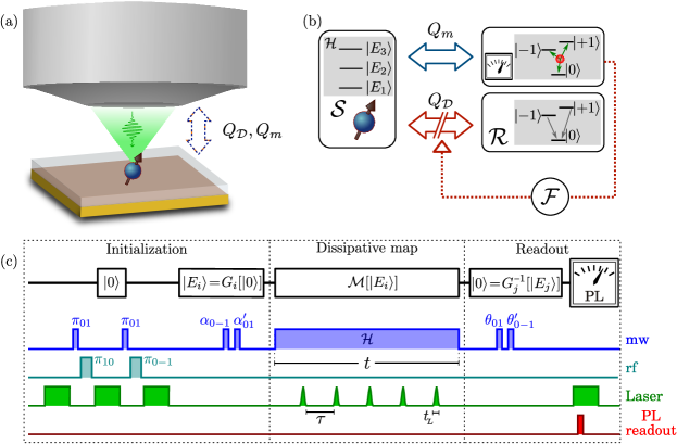
Figure 1: (a,b) Scheme of the spin system $\mathcal{S}$ in the presence of a green laser. Upon interaction with a laser pulse, the spin is subject to a quantum measurement ($Q_{m}$) of $S_{z}$, and dissipation ($Q_{\mathcal{D}}$) towards the $m_{S}=0$ spin projection. This irreversible dissipation is analogous to put the system in contact with an out-of-equilibrium reservoir $\mathcal{R}$. Since the interaction between the system and the reservoir is conditioned by the application of a quantum measurement, the dissipation acts as an intrinsic feedback mechanism. The unitary part of the dynamics is defined by the Hamiltonian $\mathcal{H}$, with eigenstates $\ket{E_{i}}$, $i=1,2,3$. (c) Scheme to measure energy conditional probabilities. The stochastic-dissipative map $\mathcal{M}$ is a combination of a train of $N_{\mathrm{L}}$ equidistant short laser pulses and a continuous driving under the Hamiltonian $\mathcal{H}$ that can be either $\mathcal{H}_{\mathrm{NV}}$ or $\mathcal{H}_{\mathrm{mw}}$ (see text). The total time of the experiment $t=N_{\mathrm{L}}\tau$ is defined in terms of the number of laser pulses and the time $\tau$ between them. The laser pulse duration $t_{\mathrm{L}}$ is negligible with respect to the continuous driving. The gates $G_{i}:\ket{0}\rightarrow\ket{E_{i}}$ and $G_{j}^{-1}:\ket{E_{j}}\rightarrow\ket{0}$ enable to prepare and readout the Hamiltonian eigenstates, respectively, by exploiting the optical properties of the NV center.

I Introduction

The Maxwell’s demon paradox, introduced by Maxwell in 1867 to discuss the validity of the second law of thermodynamics, has uncovered the relationship between thermodynamics and information, and still flourishes in modern physics Maruyama et al. (2009). The demon is an intelligent entity that uses the information resulting from the measurement of a system to condition the system dynamics, with results that may be in apparent contrast with the second law. One century later, Landauer and Bennett Bennett (1982), the fathers of so-called information thermodynamics, provided the solution of this paradox, by suggesting to consider in the thermodynamic balance also the information stored in the demon memory, which is erased in the process. The modern formulation of Maxwell’s demons is embodied by the combination of measurement and feedback control, a typical setting of information thermodynamics Funo et al. (2018); Koski et al. (2014); Naghiloo et al. (2018). The feedback mechanism can be either operated by an external agent or even performed internally, with no microscopic information exiting the system Mandal and Jarzynski (2012); Kutvonen et al. (2016). The demon can accomplish different tasks, e.g., acting to perform information heat engines, refrigerators, thermal accelerators, or heaters Buffoni et al. (2019). In quantum settings, projective measurements contribute as a purely quantum component to heat exchange Elouard et al. (2017a); Gherardini et al. (2018), and enable the feedback mechanism that the demon exploits to convert information into usable energy Toyabe et al. (2010); Masuyama et al. (2018). This feedback mechanism plays a crucial role in the investigation of quantum information thermodynamics and may find applications in information-powered quantum refrigerator or heat engine Koski et al. (2015); Elouard et al. (2017b), quantum heat transport Campisi et al. (2017), quantum computation and error correction Schindler et al. (2011), and metrology Hirose and Cappellaro (2016). Experimental implementations of Maxwell’s demons in the quantum regime have been carried out in NMR setup to compensate entropy production Camati et al. (2016), photonic platform working at the few-photons level Vidrighin et al. (2016), superconducting QED circuits Cottet et al. (2017); Naghiloo et al. (2018); Song et al. (2021), solid state spins Ji et al. (2022), and single Rydberg atoms Najera-Santos et al. (2020).

A Maxwell demon generally acts via unitary evolutions. However, a proper control and design of the system-environment coupling via the combination of coherent and non-unitary operations can be a fundamental resource for quantum information processing Verstraete et al. (2009); Pastawski et al. (2011) and thermodynamics Scarani et al. (2002); Nandkishore and Huse (2015); Strasberg et al. (2017), and more broadly for quantum simulation Barreiro et al. (2011) and sensing Do et al. (2019); Wolski et al. (2020); Xie et al. (2020). Dissipative operations can be used to produce quantum states of interest such as non-equilibrium steady states, strongly correlated states, or to prepare and stabilize robust phases and entanglement Lin et al. (2013); Barontini et al. (2015); Biella et al. (2017); Lu et al. (2017); Ma et al. (2019). A relevant feature of dissipative dynamics is the appearance of stationary states, non necessarily in thermal equilibrium Benatti and Floreanini (2003); Dutta and Cooper (2021), as a generalization of thermalization processes. Among dissipative processes, optical pumping exhibits the peculiar properties of leading the quantum system to a dissipated out-of-equilibrium state that does not depend on the system initialization. As we will show, repetitive system-environment interactions via optical pumping can be modelled as an autonomous Maxwell demon where dissipation is conditioned on the absorption of light.

Information and energy exchanges of an open quantum system with its environment inherently involve fluctuations. Quantum measurements, randomizing the system evolution, introduce quantum energy fluctuations, which impact the observable distribution obtained by averaging over many quantum trajectories Gisin (1984); Jacobs (2014). These fluctuations can drive the quantum system towards novel—often out-of-equilibrium—dynamical regimes that could not be otherwise achieved. Quantum fluctuation relations Esposito et al. (2009); Campisi et al. (2011) provide a powerful framework to characterize such energy fluctuations in thermodynamic processes. Experimental investigations of quantum fluctuation relations have been recently conducted on different platforms, including single trapped ions An et al. (2015); Smith et al. (2018), NMR systems Batalhão et al. (2014); Pal et al. (2019), atom chip Cerisola et al. (2017), superconducting qubits Zhang et al. (2018), Nitrogen-Vacancy (NV) centers in diamond Hernández-Gómez et al. (2020), and entangled photon pairs Ribeiro et al. (2020). These studies cover closed system dynamics An et al. (2015); Smith et al. (2018); Batalhão et al. (2014); Cerisola et al. (2017); Zhang et al. (2018), and certain open dynamics Smith et al. (2018); Pal et al. (2019); Hernández-Gómez et al. (2020); Ribeiro et al. (2020) where micro-reversibility may not be satisfied.

Here, we realize an autonomous dissipative Maxwell demon with a spin qutrit formed by a Nitrogen-Vacancy (NV) center in diamond at room temperature, and we investigate its purely quantum (non-Gibbsian) energy fluctuations through a generalized Sagawa-Ueda-Tasaki (SUT) quantum fluctuation relation. The intrinsic feedback mechanism acting on a dissipative dynamics is achieved by performing random projective measurements followed by conditioned and tunable optical pumping. The resulting dynamics generates non-thermal steady states in the energy basis, independent of the initial state. In the case of conditioned unitary evolution, the SUT relation establishes a fundamental connection between the thermodynamic properties of non-equilibrium quantum processes and information-theoretic quantities, evaluated by measuring and manipulating the system Sagawa and Ueda (2008); Morikuni and Tasaki (2011); Funo et al. (2013, 2015). The SUT relation has been generalized to completely positive trace-preserving (CPTP) maps Kafri and Deffner (2012); Rastegin (2013); Albash et al. (2013); Goold et al. (2015); Song et al. (2021). Our work formulates such relation in the case of conditioned dissipative dynamics and verifies it experimentally by measuring the energy change statistics of the spin qutrit. Interestingly, we find that expressing the SUT relation in the framework of the superoperators’ formalism Havel (2003) renders the computation of all the system trajectories unnecessary, drastically reducing the required computational resources. This is a relevant feature in protocols involving repeated measurements. We also measure the mean energy change of the qutrit and compare it with theoretical bounds. Finally, we find that the knowledge of the stationary state is sufficient to characterize the demon in terms of its capacity of energy extraction, without requiring any additional information on the map.

The paper is structured as follows: In Sec. II we introduce the experimental platform and the implementation of the intrinsic feedback dissipative mechanism for a spin qutrit. We discuss the formalism to model the dynamics of the qutrit as an autonomous Maxwell demon in Sec. III. Sec. IV contains a discussion about the SUT fluctuation relation and its extension beyond unitary dynamics. In Sec. V we present the experimental protocol to measure the energy variation of the spin qutrit due to the action of the dissipative-autonomous Maxwell demon. We also present and discuss our experimental results. A brief discussion about the energy extraction capability of dissipative demons is presented in Sec. VI. Conclusions and perspectives are summarized in Sec. VII.

II Feedback-controlled dissipative dynamics: Experiment

We now describe the intrinsic-feedback dissipative dynamics realized with a diamond spin qutrit.

The negatively-charged NV center, a quantum defect comprising a substitutional nitrogen atom next to a vacancy in the diamond lattice, forms an electronic spin triplet $S=1$ in its orbital ground state. The intrinsic electron spin-spin interaction separates in energy the state $\ket{m_{S}=0}$ from the degenerate $\ket{m_{S}=\pm 1}$ (where $\ket{m_{S}}$ are the eigenstates of the spin operator $S_{z}=\ket{+1}\!\!\bra{+1}-\ket{-1}\!\!\bra{-1}$ along the NV symmetry axis $z$), while an applied magnetic field $B$ aligned along $z$ removes the degeneracy of the electronic spin states $\ket{\pm 1}$, and leads to the formation of a three-level system. Each of the three states $\ket{m_{S}}$ is further split into hyperfine sublevels due to coupling to the NV ¹⁴N nuclear spin $I=1$ Steiner et al. (2010), however we restrict our analysis to the hyperfine subspace with nuclear spin projection $m_{I}=+1$, since the other states are depleted as a part of the initialization procedure and then are out of resonance in the following experiments, thus not contributing to the spin dynamics.

The spin qutrit is coherently driven by bichromatic on-resonant microwave radiation, with frequency components $\omega_{\pm 1}$. The spin dynamics under the continuous double driving is described by the Hamiltonian $H(t)=\mathcal{H}_{\mathrm{NV}}+\omega\left[\cos(\omega_{+1}t)\ket{+1}\!\!\bra{0}+\cos(\omega_{-1}t)\ket{-1}\!\!\bra{0}+h.c.\right]$, where $\omega$ is the driving Rabi frequency. When $\omega$ vanishes, this reduces to the intrinsic spin-1 Hamiltonian

$$\mathcal{H}_{\mathrm{NV}}=\Delta S_{z}^{2}+\gamma_{e}BS_{z}\,,$$ (1)

where $\Delta\simeq 2.87$ GHz is the zero-field-splitting, and $\gamma_{e}$ is the electron gyromagnetic ratio ($\hbar=1$ here and throughout this paper) . When the microwave (mw) driving is on, with $\omega_{\pm 1}=\Delta\pm\gamma_{e}B$, in the mw rotating frame and after applying the rotating-wave approximation the spin Hamiltonian simplifies as follows:

$$\mathcal{H}_{\mathrm{mw}}=\omega S_{x}.$$ (2)

We performed different experiments while using each of the two Hamiltonians [Eq. (1) and (2)] to determine the unitary part of dissipative maps, and the energy basis in which fluctuations are evaluated.

On top of the unitary evolution, the system is intermittently opened by means of its interaction with a train of short laser pulses. The pulse length $t_{\mathrm{L}}$ is negligible compared to the characteristic timescale of the spin dynamics ($t_{\mathrm{L}}\ll 2\pi/\omega$). Although the laser pulses are equidistant, photon absorption events follow a binomial random distribution in time, due to the finite photon absorption probability ($p_{\mathrm{a}}<1$). While a long laser pulse would produce a complete optical pumping in the $\ket{0}$ state Doherty et al. (2013), the interaction with a short laser pulse—as used here— has the following effect: If photons are not absorbed, the state of the system is unperturbed; if a photon is absorbed, the spin performs an optical transition to a short-lifetime orbital excited triplet state, loosing any coherence in the $S_{z}$-basis during the process Wolters et al. (2013), then it decays back to the orbital ground triplet state $\{\ket{\pm 1},\ket{0}\}$. The decay occurs through a direct spin-preserving radiative channel, or through spin-nonpreserving nonradiative paths involving intermediate metastable states. The different decay rates of radiative and nonradiative paths result in an optical-pump of the spin towards the state $\ket{0}$. Considering the reduced 3-level system formed by the spin levels of the orbital ground state, the photon absorption induces a loss of coherence and an irreversible dissipation, originated by optical pumping. Such a dissipation, conditioned by the absorption of a photon, constitutes the basis of the intrinsic-feedback dissipative dynamics, as schematized in Fig. 1(a-b). The mathematical model of these phenomena is described in Sec. III.

III Modelled dynamics: Autonomous-dissipative Maxwell demon

Here, we model the qutrit dynamics in terms of a Lindbladian master equation describing an autonomous-dissipative Maxwell’s demon. For this we use the formalism described in Ref. Havel (2003) for superoperators represented as $N^{2}\times N^{2}$ matrices, where $N=3$ is the dimension of the Hilbert space of the three-level system (3LS). According to this formalism, a given density matrix $\rho$ under unitary evolution $U\equiv e^{-i\tau\mathcal{H}}$ is transformed into

$$\operatorname{col}[U\rho U^{\dagger}]=\boldsymbol{U}\operatorname{col}[\rho]$$ (3)

where $\operatorname{col}[\rho]$ denotes the vectorization of $\rho$, obtained by stacking the columns of $\rho$ to form a ‘column’ vector, and $\boldsymbol{U}\equiv\exp(-i\tau(\mathcal{H}\otimes\mathbb{1}_{3\times 3}-\mathbb{1}_{3\times 3}\otimes\mathcal{H}^{*}))$ with $\otimes$ being the Kronecker product.

On the other hand, the interaction between the 3LS and a short laser pulse can be described by a positive operator-valued measure (POVM) followed by a dissipation operator conditioned on the POVM result. Specifically, the interaction with a single short laser pulse transforms a density matrix $\rho$ into

$$\operatorname{col}[\rho(t_{\mathrm{L}})]=\boldsymbol{\mathcal{A}}\operatorname{col}[\rho]$$ (4)

where the superoperator $\boldsymbol{\mathcal{A}}$ models the mean effect of the single short laser pulse. Taking into account all the possible outcomes of the 3LS-laser interaction, $\boldsymbol{\mathcal{A}}$ is written as

$$\boldsymbol{\mathcal{A}}\equiv\sum_{j=1}^{4}\boldsymbol{\mathcal{D}}_{j}\boldsymbol{m}_{j}$$ (5)

where $\boldsymbol{m}_{j}\equiv m_{j}\otimes m_{j}$ is one of the measurement super-operator associated with the POVM $m_{j}=\{m_{1},m_{2},m_{3},m_{4}\}$ with

$$m_{1} \equiv\sqrt{p_{\mathrm{a}}}\ket{-1}\!\!\bra{-1}$$ (6a)

$$m_{2} \equiv\sqrt{p_{\mathrm{a}}}\ket{0}\!\!\bra{0}$$ (6b)

$$m_{3} \equiv\sqrt{p_{\mathrm{a}}}\ket{+1}\!\!\bra{+1}$$ (6c)

$$m_{4} \equiv\sqrt{(1-p_{\mathrm{a}})}\mathbb{1}_{3\times 3},$$ (6d)

such that $\sum_{j=1}^{4}m_{j}m_{j}^{\dagger}=\mathbb{1}_{3\times 3}$, and $\boldsymbol{\mathcal{D}}_{j}$ represents the action of a superoperator conditioned to the result of the POVM:

$$\boldsymbol{\mathcal{D}}_{j}=\begin{cases}\boldsymbol{\mathbb{1}}_{9\times 9},&\text{if }j=4\\ \boldsymbol{\mathcal{L}},&\text{otherwise}\end{cases}$$ (7)

with

$$\boldsymbol{\mathcal{L}}\equiv\exp\left(t_{\mathrm{L}}\sum_{\ell=0}^{1}L^{*}_{\ell}\otimes L_{\ell}-\frac{1}{2}\mathbb{1}_{3\times 3}\otimes L^{\dagger}_{\ell}L_{\ell}\right.$$

$$\left.-\frac{1}{2}(L^{\dagger}_{\ell}L_{\ell})^{*}\otimes\mathbb{1}_{3\times 3}\right)$$ (8)

where $(\cdot)^{*}$ denotes complex conjugate, and $L_{\ell}$ are the Lindblad jump operators $\{L_{0},L_{1}\}\equiv\{\sqrt{\Gamma}\ket{0}\!\!\bra{+1},\sqrt{\Gamma}\ket{0}\!\!\bra{-1}\}$, describing the dissipation towards the state $\ket{0}$. In Eq. (5), the term for $j=4$ corresponds to the case where the laser pulse is not absorbed, while the other three terms model the absorption of a single laser pulse. The Lindblad dissipative super-operator $\boldsymbol{\mathcal{L}}$ is defined in terms of the product between the effective decay rate and the laser duration $\Gamma t_{\mathrm{L}}$, which dictates the strength of the dissipation that brings the system towards $\ket{0}$; the dissipation probability is $p_{\mathrm{d}}\equiv(1-e^{-\Gamma t_{\mathrm{L}}})$. The explicit expression of $\boldsymbol{\mathcal{L}}$ can be found in the Supplemental Material at [URL will be inserted by publisher]. Using short laser pulses with $t_{\mathrm{L}}=41$ ns, we experimentally characterized the strength of this decay rate resulting in a value such that $\Gamma t_{\mathrm{L}}\simeq 1/2$. Given the effective nature of this model, the value of $\Gamma$ might vary for different NV centers and under different experimental conditions. Notice that for a long laser pulse ($t_{\mathrm{L}}\Gamma\gg 1$) any given state $\rho$ is transformed into $\boldsymbol{\mathcal{L}}\operatorname{col}[\rho]=\operatorname{col}[\ket{0}\!\!\bra{0}]$, which is consistent with the usual protocol employed to optically initialize the electronic spin state. Note that, in the hypothetical limit where $p_{\mathrm{d}}=0$, then no dissipation will occur ($\boldsymbol{\mathcal{L}}=\boldsymbol{\mathbb{1}}_{9\times 9}$) and consequently $\boldsymbol{\mathcal{D}}_{j}=\boldsymbol{\mathbb{1}}_{9\times 9}$.

Here, the action of the dissipation operator is conditioned on the result of the previously-applied POVM. Thus, the combined effect of unitary evolution, POVMs, and dissipation results in an autonomous Maxwell’s demon, whose action is defined by the specific photodynamics of the NV center [see Fig. 1(b)]. Overall, the effect of this feedback-controlled dissipative map $\mathcal{M}$, after $N_{\mathrm{L}}$ laser pulses, is thus modeled as $\mathcal{M}[\rho]\rightarrow\boldsymbol{\mathcal{B}}^{N_{\mathrm{L}}}\operatorname{col}[\rho]$, where $\boldsymbol{\mathcal{B}}$ is the superoperator that describes a single block of the dynamics formed by unitary evolution followed by the interaction of the system with a short laser pulse

$$\boldsymbol{\mathcal{B}}\equiv\boldsymbol{\mathcal{A}}\,\boldsymbol{U}.$$ (9)

The study of energy variation fluctuations induced by this autonomous Maxwell demon is a central issue of this article.

IV Dissipative Sagawa-Ueda-Tasaki relation

In this context, quantum fluctuation relations (QFR) Campisi et al. (2011) provide a powerful framework to characterize fluctuations of energy by inspecting its characteristic function. The quantum fluctuation relation for dynamics under measurements and feedback control, also known as the quantum Sagawa-Ueda-Tasaki relation, was originally proposed for protocols where specific unitary operations are applied to the quantum system depending on the outcomes of a sequence of projective measurements Morikuni and Tasaki (2011); Funo et al. (2013). Later on it was extended to the more general case of non-unitary dynamics described by completely positive trace-preserving (CPTP) maps, subject to the result of the POVMs—which generalize the projective measurements Kafri and Deffner (2012); Rastegin (2013); Albash et al. (2013); Goold et al. (2015); Song et al. (2021). Here, we detail how to formulate such extension using the superoperator formalism, instead of the usual Kraus operators formalism.

A two-point measurement (TPM) scheme Talkner et al. (2007) is used to characterize the statistics of the energy variation: An initial energy measurement projects an initial thermal state $\rho^{\mathrm{th}}$ into one of the Hamiltonian eigenstates, which then evolves under the map we are studying, and a final energy measurement allows us to extract the energy difference. By repeating this process several times it is possible to reconstruct probability distribution of the energy variation

$$P_{\Delta E}\equiv{\rm Prob}(\Delta E)=\sum_{i,j}\delta(\Delta E-\Delta E_{j,i})P_{j|i}P_{i},$$ (10)

where $\Delta E_{j,i}\equiv E_{j}-E_{i}$, $P_{i}$ is the probability to obtain $E_{i}$ as a result of the first energy measurement of $\rho^{\mathrm{th}}$, and $P_{j|i}$ is the conditional probability to obtain $E_{j}$ as a result of the second energy measurement at the end of the TPM scheme. Once that the statistics of $\Delta E$ are known, the characteristic function $\mathcal{G}(\eta)\equiv\langle e^{iu\Delta E}\rangle_{u=i\eta}$ of $P_{\Delta E}$ can be experimentally computed as

$$\mathcal{G}(\eta)=\sum_{i,j}e^{-\eta\Delta E_{j,i}}P_{j|i}P_{i}\,.$$ (11)

The general protocol is the following. An $n$-dimensional quantum system (in our experiments, $n=3$) evolves under the Hamiltonian $H_{0}$; then, a POVM is performed on the system. The quantum measurement is defined by a set of positive semidefinite operators $\Pi_{1},...\Pi_{n^{\prime}}$ such that $\sum_{k=1}^{n^{\prime}}\Pi_{k}=\mathbb{1}_{n\times n}$. According to a feedback mechanism, the measurement outcome $k$ determines the CPTP map $\Phi_{k}$ under which the system continues to evolve. Since $\Phi_{k}$ is a CPTP map, we can define the superoperator propagator $\boldsymbol{\Phi}_{k}$ such that the evolution of a generic density matrix $\rho$ is described as $\operatorname{col}[\Phi_{k}[\rho]]=\boldsymbol{\Phi}_{k}\operatorname{col}{[\rho]}$ Havel (2003). Hence, the complete feedback map $\mathcal{M}_{\Phi}$ transforms the density matrix $\rho$ into

$$\operatorname{col}[\mathcal{M}_{\Phi}[\rho]]=\sum_{k=1}^{n^{\prime}}\boldsymbol{\Phi}_{k}\boldsymbol{\Pi}_{k}\boldsymbol{U}_{0}\operatorname{col}[\rho],$$ (12)

where $\boldsymbol{U}_{0}=\exp(-it(H_{0}\otimes\mathbb{1}_{n\times n}-\mathbb{1}_{n\times n}\otimes H_{0}^{*}))$ is the superoperator that describes the unitary evolution before the POVM, and $\boldsymbol{\Pi}_{k}\equiv\Pi_{k}\otimes\Pi_{k}$ represents the action of the measurement operators on the quantum system.

As a result, the characteristic function of the energy variation is equal to a parameter $\gamma$ that represents the efficacy of the feedback mechanism:

$$\mathcal{G}(\beta)=\gamma\equiv\sum_{k=1}^{n^{\prime}}\operatorname{Tr}_{n\times n}\left[\boldsymbol{\Pi}_{k}^{\dagger}\boldsymbol{\Phi}_{k}^{\dagger}\,\operatorname{col}[\rho^{\mathrm{th}}_{\mathrm{f}}]\right],$$ (13)

where $\beta$ is the inverse temperature of the initial thermal state, $\rho^{\mathrm{th}}_{\mathrm{f}}$ is a thermal state at the final time of the TPM scheme, the symbol $\dagger$ denotes conjugate-transpose, and $\operatorname{Tr}_{n\times n}[\operatorname{col}[\cdot]]\equiv\operatorname{Tr}[\cdot]$. The efficacy of the feedback mechanism, as measured by $-\ln\gamma$, determines a lower bound on the energy variation of the system, as we will discuss in Sec. VI. The mathematical proof of Eq. (13) can be found in Appendix A (see Corollary 1). The proof is based on the fact that the map $\mathcal{M}_{\Phi}$ is itself a CPTP map, meaning that Eq. (13) is a particular case of the general quantum fluctuation relation for CPTP maps Kafri and Deffner (2012); Rastegin (2013); Albash et al. (2013); Rastegin and Życzkowski (2014); Goold et al. (2015); Song et al. (2021). It is worth observing that Eq. (13) reduces to the original quantum SUT relation Morikuni and Tasaki (2011) in the particular case where the intermediate quantum measurements are projective and $\Phi_{k}$ are unitary evolution operators. Moreover, if $\Phi_{k}$ are unital CPTP maps, then $\boldsymbol{\Phi}_{k}^{\dagger}$ is trace preserving Havel (2003), hence $\gamma=1$ Kafri and Deffner (2012); Albash et al. (2013) for any time-independent Hamiltonian. In contrast, for non-unital maps where microreversibility is not satisfied, the value of $\gamma$ can be different from $1$ and, in general, involves non trace-preserving operators $\boldsymbol{\Phi}_{k}^{\dagger}$.

Equations (12) and (13) refer to a feedback operation on the quantum system enabled by applying a single POVM measurement, and they can be simplified by defining $\boldsymbol{\mathcal{B}}_{\Phi}\equiv\sum_{k=1}^{n^{\prime}}\boldsymbol{\Phi}_{k}\boldsymbol{\Pi}_{k}$ that leads to $\gamma=\operatorname{Tr}_{n\times n}[\boldsymbol{\mathcal{B}}_{\Phi}^{\dagger}\,\operatorname{col}[\rho^{\mathrm{th}}]]$. Therefore, extending the protocol to the scenario where measurements and feedback are applied repeatedly is quite straightforward: After $N$ repetitions $\gamma=\operatorname{Tr}_{n\times n}[(\boldsymbol{\mathcal{B}}_{\Phi}^{\dagger})^{N}\,\operatorname{col}[\rho^{\mathrm{th}}]]$. Expressing $\gamma$ in this way significantly simplifies its computation, because it removes the requirement to calculate every possible quantum trajectory originated by the system dynamics; compare for example with Refs. Morikuni and Tasaki (2011); Campisi et al. (2017). This advantage may be significant since the number of trajectories scales exponentially with the number of measurements. In addition, for any CPTP dissipative map, whereby the system asymptotically reaches the single steady state $\operatorname{col}[\rho^{\infty}]\equiv\lim_{N\rightarrow\infty}(\boldsymbol{\mathcal{B}}_{\Phi})^{N}\operatorname{col}[\rho]$, for a generic initial state $\rho$, we can write the asymptotic value of $\gamma$ as (see also Corollary 2 in Appendix A)

$$\gamma^{\infty}\equiv\lim_{t\rightarrow\infty}\gamma=n\langle\rho^{\infty},\rho^{\mathrm{th}}\rangle_{\mathrm{hs}}$$ (14)

where $\langle\rho_{1},\rho_{2}\rangle_{\mathrm{hs}}\equiv\operatorname{Tr}[\rho_{1}^{\dagger}\rho_{2}]$ denotes the Hilbert-Schmidt inner product, and $n$ is the dimension of the quantum system. Remarkably, the quantity in Eq. (14) can be measured experimentally, even for non-unital maps.

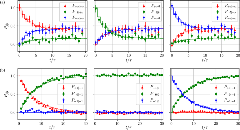
Figure 2: Dynamics of the spin qutrit under the autonomous-dissipative Maxwell demon. The probability $P_{j|i}$ of measuring the state $\ket{E_{j}}$ after applying the map $\mathcal{M}$ to the state $\ket{E_{i}}$ is shown as a function of the number of laser pulses $N_{\mathrm{L}}=t/\tau$, where $\ket{E_{i}}$ and $\ket{E_{j}}$ represent each of the eigenstates of the $3LS$ Hamiltonian (a) $\mathcal{H}_{\mathrm{mw}}$ and (b) $\mathcal{H}_{\mathrm{NV}}$. In both cases, the duration of the laser pulses is $t_{\mathrm{L}}=41$ ns, and the time between pulses is $\tau=424$ ns. Each panel corresponds to a different initial eigenstate: (a) $\{\ket{+\omega},\ket{\emptyset},\ket{-\omega}\}$ and (b) $\{\ket{+1},\ket{0},\ket{-1}\}$. The markers with errorbars represent the experimental data, and each solid line corresponds to the calculation performed with the theoretical model of the map $\mathcal{M}$, as described in Sec. III. Experimental error bars are mainly due to photon shot noise. Notice that these measurement stem from a comparison between the PL of the two reference states and the PL of the NV after the studied dynamics, which may result in values that are slightly outside the $[0,1]$ interval.

V Dynamics and thermodynamics of the demon

We have characterized the dynamics and the quantum (non-thermal) energy fluctuations of the 3-level spin system induced by non-unital quantum dissipative maps in two independent experiments:

1. Coherent double driving and short laser pulses. The unitary part of the map $\mathcal{M}$ is ruled by the Hamiltonian $\mathcal{H}_{\mathrm{mw}}$ defined in Eq. (2), with eigenstates $\ket{E_{1}}=\ket{-\omega}$, $\ket{E_{2}}=\ket{\emptyset}$, and $\ket{E_{3}}=\ket{+\omega}$, where $\ket{\pm\omega}\equiv\frac{1}{2}\left(\ket{-1}\pm\sqrt{2}\ket{0}+\ket{1}\right)$, and $\ket{\emptyset}\equiv\frac{1}{\sqrt{2}}\left(\ket{-1}-\ket{1}\right)$.

2. Undriven spin, subject to short laser pulses. The spin Hamiltonian is $\mathcal{H}_{\mathrm{NV}}$ with eigenstates $\ket{E_{1}}=\ket{0}$, $\ket{E_{2}}=\ket{-1}$, and $\ket{E_{3}}=\ket{+1}$.

The effect of the map $\mathcal{M}$ on the spin energy is characterized by measuring the energy jump probabilities, i.e., the conditional probabilities associated with the energy variation in a given time interval. The scheme used to measure conditional probabilities, as depicted in Fig. 1(c) consists in the following steps:

a) Initialize the system into one of the Hamiltonian eigenstates, say $\ket{E_{i}}$;

b) Evolve the system under the map $\mathcal{M}$ up to time $t$;

c) Read out the probability of the spin to be in the Hamiltonian eigenstate $\ket{E_{j}}$ at final time $t$;

d) Repeat the procedure for each initial and final Hamiltonian eigenstates.

V.1 Spin initialization and readout

The NV spin is initially prepared in the spin qutrit Hamitonian eigenstate $\ket{E_{i}}$. The starting point of the initialization is a thermal spin mixture $\overline{\rho}=\sum_{m_{S},m_{I}}\ket{m_{S},m_{I}}\!\!\bra{m_{S},m_{I}}$ within the $9\times 9$ space described by the hyperfine manifold within orbital ground state. The quantum gate $G_{0}$ prepares the hyperfine state $\ket{m_{S},m_{I}}\equiv\ket{0,1}$ (see Fig. 1). From now on we drop the hyperfine spin to simplify the notation, $\ket{m_{S},1}=\ket{m_{S}}$. The details about the nuclear spin initialization can be found in the Supplemental Material at [URL will be inserted by publisher]. Pure electron spin states in the energy basis ($\ket{E_{i}}$) are then prepared by applying opportune two-level-system quantum gates ($G_{i}$, in Fig. 1) realized by means of nuclear spin selective monochromatic microwave pulses resonant with the electronic transitions $\ket{0}\rightarrow\ket{+1}$ or $\ket{0}\rightarrow\ket{-1}$ as described in Appendix B.

After a spin evolution under the dissipative map $\mathcal{M}$, the spin state readout is performed by exploiting the difference in the NV center photoluminescence (PL) intensity, among state $\ket{0}$ and states $\ket{\pm 1}$, upon illumination with green laser light. To measure the probability of the spin state to be equal to each of the three Hamiltonian eigenstates $\ket{E_{j}}$ at the end of the protocol, that eigenstate is projected into the $S_{z}$ eigenstate $\ket{0}$ (quantum gate $G_{j}^{-1}$ in Fig. 1), then the PL intensity is recorded. The description of the gates $G_{i}$ and $G_{j}^{-1}$ for each of the initial and final eigenstates can be found in Appendix B. Since the readout process is destructive, each experiment is composed by three different runs, where the probability of each of the three eigenstates is recorded. Due to limited diamond PL collection efficiency and to photon shot noise, each experiment is repeated $\sim 10^{6}$ times.

Notice that the duration of each realization of the experiment is much shorter than the nuclear spin lifetime so that the three-dimensional hyperfine spin subspace is well defined for the whole experiment duration.

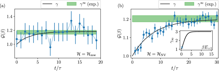
Figure 3: Experimental verification of the generalized quantum Sagawa-Ueda-Tasaki relation (13) for a 3LS controlled by an autonomous-dissipative Maxwell’s demon. The energy variation statistics are shown in terms of the total time of the experiment divided by the time between laser pulses, i.e. in terms of the number of laser pulses $N_{\mathrm{L}}=t/\tau$. (a) The continuous coherent driving of the 3LS is defined by the Hamiltonian $\mathcal{H}_{\mathrm{mw}}$ and the value of the inverse temperature of the initial state is $\beta=3/E_{+\omega}$. (b) Same as (a) but for a Hamiltonian $\mathcal{H}_{\mathrm{NV}}$, and an inverse temperature of the initial state $\beta=0.297/E_{+1}$. Blue circles represent the measured values of the characteristic function $\mathcal{G}(\beta)$, the black continuous line denotes the theoretical estimation of $\gamma$ [Eq. (15)], and the green area marks the experimental value of $\gamma^{\infty}$ [Eq. (14)], the asymptotic value of $\gamma$. Inset: theoretical value of $\gamma^{\infty}$ as a function of the initial inverse temperature $\beta$. The blue cross is associated with the value of $\beta$ used for the experimental data in (b).

V.2 Demon dynamics

We then reconstruct the dynamics of the spin qutrit under the autonomous-dissipative Maxwell’s demon. The conditional probabilities $P_{j|i}$ associated with energy jumps from the initial ($\ket{E_{i}}$) to the final ($\ket{E_{j}}$) eigenstates are shown in Fig. 2, as a function of the number of laser pulses applied before performing the readout. The experimental data are shown together with the theoretical model of the dynamics, described in Sec. III. The excellent agreement between experiment and theory leads us to conclude that the dynamics of the system is very well described by an autonomous feedback mechanism. The results show that the conditional probabilities $P_{j|i}$ tend to a single constant value in the long-time regime (large $N_{\mathrm{L}}$). In other words, the spin state asymptotically approaches a steady state in the energy basis (SSE) that does not depend on the initial state, thus confirming the dissipative nature of the map $\mathcal{M}$. In the case of $\mathcal{H}=\mathcal{H}_{\mathrm{NV}}$ [Fig. 2(b)], the asymptotic state is $\rho^{\infty}_{\mathrm{NV}}=\sum_{\ell=-1}^{+1}p^{\infty}_{\ell}\ket{\ell}\!\!\bra{\ell}$, with populations, obtained from the experimental data, $p^{\infty}_{+1}=(-0.01\pm 0.01)$, $p^{\infty}_{0}=(1.01\pm 0.01)$, and $p^{\infty}_{-1}=(0.00\pm 0.01)$. In such case the protocol is asymptotically equivalent to an initialization procedure into $\rho^{\infty}_{\mathrm{NV}}=\ket{0}\!\!\bra{0}$. On the other hand, if $\mathcal{H}=\mathcal{H}_{\mathrm{mw}}$ [Fig. 2(a)], the asymptotic state significantly differ from $\ket{0}=\frac{1}{\sqrt{2}}\left(\ket{+\omega}-\ket{-\omega}\right)$. Although the interaction with each laser pulse pushes the system towards $\ket{0}$, the unitary evolution modifies the density operator populations in the $S_{z}$ basis, thus changing the SSE at large times. In such case, the asymptotic state is $\rho^{\infty}_{\mathrm{mw}}=\sum_{\ell=-\omega}^{+\omega}p^{\infty}_{\ell}\ket{\ell}\!\!\bra{\ell}$, with populations, obtained from the experimental data, $p^{\infty}_{+\omega}=(0.41\pm 0.01)$, $p^{\infty}_{\emptyset}=(0.20\pm 0.02)$, and $p^{\infty}_{-\omega}=(0.40\pm 0.01)$, as shown in Fig. 2(a).

V.3 Energy variation distribution

Based on the formalism established in Sec. IV, here we study the statistics of the energy exchange fluctuations of the demon and we calculate the feedback efficacy for the specific map $\mathcal{M}$.

For an initial thermal state, measuring the conditional probabilities $P_{j|i}$ gives access to the probability distribution of the energy variation $P_{\Delta E}$, as defined in Eq. (10). We remind that in the usual two-point measurement (TPM) scheme Talkner et al. (2007), the probability $P_{i}$ is measured by performing an energy projective measurement on the initial state. Here, we initialize the spin into each of the eigenstates of the Hamiltonian [Sec. V], and we obtain mixed (equilibrium) states as statistical mixture of the eigenstates with probabilities $P_{i}$ as weight factors. Our scheme gives equivalent results to a TPM scheme, owing to the large number of experimental realizations Hernández-Gómez et al. (2020); Cimini et al. (2020), while overcoming the difficulties to prepare an initial thermal state. Moreover, our scheme removes possible experimental errors inherent in the first energy measurement, and allows to use one single set of measurements to study different initial states.

Once that we have measured the energy variation distribution $P_{\Delta E}$, we can experimentally compute the values of the characteristic function $\mathcal{G}(\eta)$ as in Eq. (11). In addition, as pointed out in Sec. IV, the value of $\gamma^{\infty}$ can be independently computed from the initial and asymptotic states of the map [Eq. (14)]. The measurements of $\mathcal{G}(\beta)$ and $\gamma^{\infty}$ are shown in Fig. 3. The agreement between the measured values of these two parameters represents the experimental verification of the generalized SUT fluctuation relation [Eq. (13)], in the SSE regime, for an open three-level system under quantum (non-thermalizing) dissipative dynamics conditioned by POVM quantum measurements. Let us observe that the theoretical model of the map $\mathcal{M}$ [Sec. III] allows us to calculate the efficacy $\gamma$ also in the transient regime, as

$$\gamma=\operatorname{Tr}_{3\times 3}\left[(\boldsymbol{\mathcal{B}}^{\dagger})^{N_{\mathrm{L}}}\,\operatorname{col}[\rho^{\mathrm{th}}]\right]$$ (15)

with $\boldsymbol{\mathcal{B}}$ defined in Eq. (9). Here, it is worth noting that the ‘backwards’ superoperator $\boldsymbol{\mathcal{B}}^{\dagger}$ is not trace preserving, a clear sign of the non-reversibility associated with the dissipative process Campisi et al. (2017). In the transient regime, the values of $\gamma$ [Eq. (15)] were compared with the experimental values of the characteristic function $\mathcal{G}(\beta)$, as a function of the number of laser pulses. As shown in Fig. 3(a-b), there is an excellent agreement between the two quantities.

In the specific case of $\mathcal{H}=\mathcal{H}_{\mathrm{NV}}$, where the Hamiltonian commutes with the POVM operators and with the dissipative operator, we can derive an analytic expression for the efficacy $\gamma$ defined in Eq. (15) as

$$\gamma=\mu^{N_{\mathrm{L}}}+3(1-\mu^{N_{\mathrm{L}}})e^{\beta F}$$ (16)

where $F\equiv-\beta^{-1}\ln Z$ is the initial free energy of the system, with $Z\equiv\sum_{k=-1}^{1}e^{-\beta E_{i}}$, and $\mu\equiv 1-p_{\mathrm{d}}p_{\mathrm{a}}\in[0,1]$ defines the probability for the system to not be subjected to feedback. We also recall that $p_{\mathrm{a}}$ denotes the laser pulse absorption probability, and $p_{\mathrm{d}}\equiv(1-e^{-t_{\mathrm{L}}\Gamma})$ is the dissipation probability for the interaction with a single laser pulse [Sec III]. The derivation of Eq. (16) is given in the Supplemental Material at [URL will be inserted by publisher]. As one would expect, $\gamma=1$ if $p_{\mathrm{a}}=0$ (closed quantum system), or in case of pure projective measurements without dissipation $e^{-t_{\mathrm{L}}\Gamma}=1$ (no feedback). In addition, since $Z<3$ for $\beta\neq 0$, Eq. (16) implies that $\gamma>1$, a necessary condition for energy extraction Campisi et al. (2017) (see also Sec. VI). As final remark, notice that $\gamma$ in Eq. (16) is defined in terms of macroscopic quantities – it does not depend on the trajectories followed by the system. In the inset of Fig. 3(b), we show the behavior of the asymptotic value of $\gamma^{\infty}=3\,e^{\beta F}$ obtained from Eq. (16) in the SSE regime, as a function of the inverse initial temperature $\beta$. This result is in agreement with Eq. (14) for the asymptotic state $\rho^{\infty}_{\mathrm{NV}}=\ket{0}\!\!\bra{0}$.

VI Extractable energy in autonomous-dissipative demons

In this section, we characterize the Maxwell’s demon in terms of its capability of energy extraction.

The mean energy variation originated by the demon is defined as $\langle\Delta E\rangle\equiv\int\Delta EP_{\Delta E}\,d\Delta E$, which can be rewritten as $\langle\Delta E\rangle=\sum_{i,j}(E_{j}-E_{i})P_{j|i}P_{i}$ using Eq. (10). Negative values of $\langle\Delta E\rangle$ denote the extraction of energy from the system. The maximal amount of extractable energy ($-\langle\Delta E\rangle$) is expected to be bounded from above Morikuni and Tasaki (2011); Campisi et al. (2017) by two fundamental quantities, $\ln\gamma$ and the classical mutual information $\mathcal{I}$ that measures the degree of correlation between the actual outcomes of the POVMs and the outcomes recorded by the demon. In the case of an autonomous demon – where no microscopic information needs to be read out by an external agent during the feedback process – no errors are associated with the intermediate measurements. In this error-free limit the mutual information $\mathcal{I}$ reduces to the Shannon entropy Morikuni and Tasaki (2011), i.e., the measurement of the degree of correlation between the trajectories of the system. For a quantum dynamics under the action of measurements and feedback, each sequence of measurements $(k_{1},\ldots,k_{N_{L}})$ corresponds to a different quantum trajectory. Thus, formally one has that in the error-free limit

$$\mathcal{I}\longrightarrow\langle S_{k_{1},\ldots,k_{N_{L}}}\rangle=$$

$$\displaystyle{-\sum_{k_{1},\ldots,k_{N_{L}}}p(k_{1},\ldots,k_{N_{L}})\ln p(k_{1},\ldots,k_{N_{L}})}$$ (17)

where $\langle S_{k_{1},\ldots,k_{N_{L}}}\rangle$ is the Shannon entropy, and $p(k_{1},\ldots,k_{N_{L}})$ is the probability for the system to follow the $(k_{1},\ldots,k_{N_{L}})$ trajectory. This probability is defined as

$$p(k_{1},\ldots,k_{N_{L}})=\operatorname{Tr}_{n\times n}[ \boldsymbol{m}_{k_{N_{L}}}\boldsymbol{U}\boldsymbol{\mathcal{D}}_{k_{N_{L}-1}}\boldsymbol{m}_{k_{N_{L}-1}}\boldsymbol{U}\cdots$$

$$\cdots\boldsymbol{\mathcal{D}}_{k_{1}}\boldsymbol{m}_{k_{1}}\boldsymbol{U}\,\operatorname{col}[\rho^{\mathrm{th}}]],$$ (18)

where each $k_{i}$ can take the values $\{1,2,3,4\}$ that indicate one of the results of the $i-$th POVM, as described by Eqs. (6).

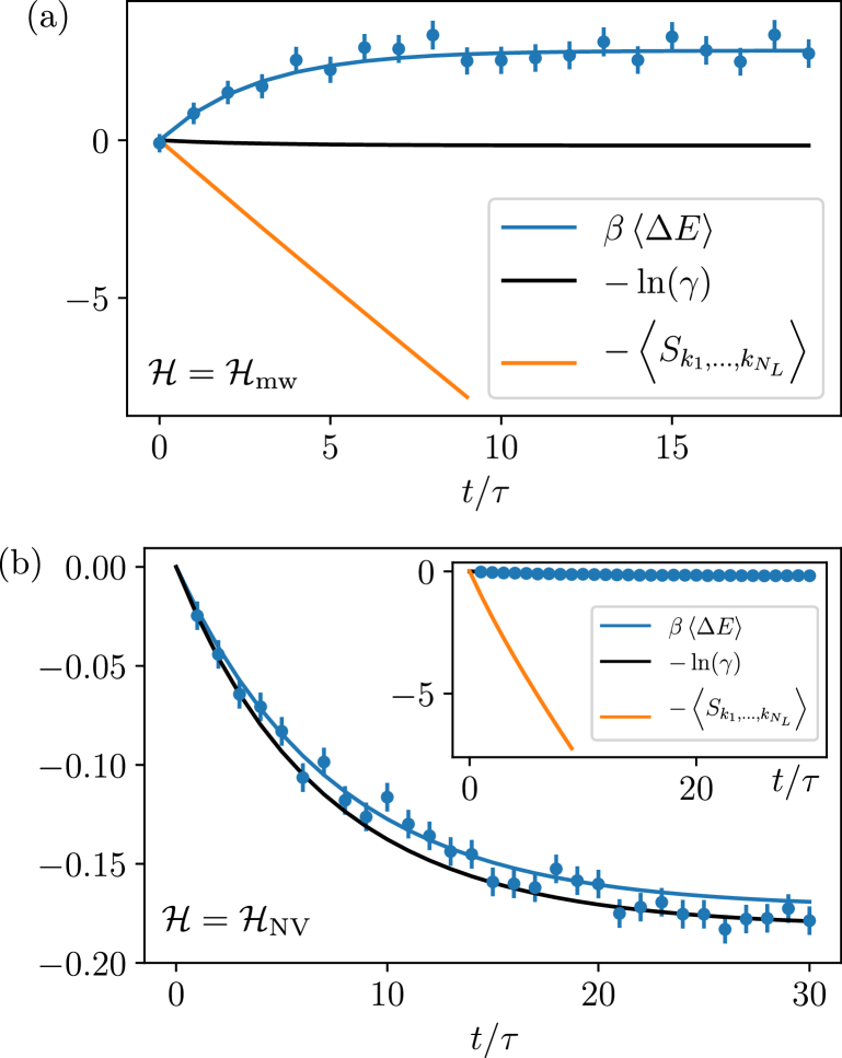
Figure 4: Experimental values of $\beta\langle\Delta E\rangle$ as a function of the number of laser pulses, for a 3LS with Hamiltonian operators $\mathcal{H}_{\mathrm{mw}}$ (a) and $\mathcal{H}_{\mathrm{NV}}$ (b). Negative values of $\beta\langle\Delta E\rangle$ (with $\beta>0$) may allow for energy extraction from the 3LS. The solid blue line corresponds to the values of $\beta\langle\Delta E\rangle$ as predicted by theory, while the theoretical bounds $-\ln\gamma$ and $-\langle S_{k_{1},\dots,k_{N_{L}}}\rangle$ are denoted by solid black and orange lines, respectively. The inset in (b) shows at the same time the tightness of $-\ln\gamma$ and the discrepancy of $-\langle S_{k_{1},\dots,k_{N_{L}}}\rangle$, both with respect to the mean energy variation $\beta\langle\Delta E\rangle$.

In Fig. 4 we compare the experimental values of $\beta\langle\Delta E\rangle$ (with fixed inverse temperature $\beta>0$) with the calculation of $-\ln\gamma$ and $-\mathcal{I}$, as a function of the number of laser pulses. Note that the number of trajectories grows as $4^{N_{\mathrm{L}}}$, therefore the exact estimation of $\mathcal{I}$ becomes impractical for large $N_{\mathrm{L}}$. In Fig. 4 we show the exact values of $-\mathcal{I}$ for $N_{\mathrm{L}}<10$ (up to $\sim 2.6\times 10^{5}$ trajectories). In contrast, $\langle\Delta E\rangle$ and $\gamma$ do not require the computation of single trajectories, since they are simply determined in terms of $\boldsymbol{\mathcal{B}}^{N_{\mathrm{L}}}$ and $(\boldsymbol{\mathcal{B}}^{\dagger})^{N_{\mathrm{L}}}$ respectively. In the case where $\mathcal{H}=\mathcal{H}_{\mathrm{mw}}$, energy extraction does not occur (indeed, $\beta\langle\Delta E\rangle>0$). In contrast, in the case $\mathcal{H}=\mathcal{H}_{\mathrm{NV}}$, $\beta\langle\Delta E\rangle<0$ for any time $t>0$. Moreover, one can observe that even experimentally the inequality

$$\beta\langle\Delta E\rangle\geq\max\left\{-\ln\gamma,-\langle S_{k_{1},\ldots,k_{N_{L}}}\rangle\right\}$$ (19)

is always validated for any value of $t$. However, in both experimental scenarios, the tightest bound is provided by $\ln\gamma$.

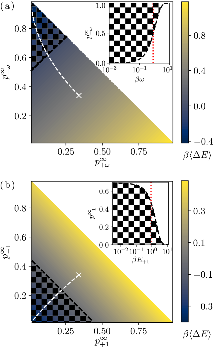
Figure 5: Values of $\beta\langle\Delta E\rangle$ as a function of the asymptotic state populations, for $\mathcal{H}=\mathcal{H}_{\mathrm{mw}}$ (a) and for $\mathcal{H}=\mathcal{H}_{\mathrm{NV}}$ (b). In these plots, each point represents a different asymptotic state of the generic quantum dissipative map $\Phi_{\mathrm{d}}$. The white cross represents a completely mixed asymptotic state for a 3LS, corresponding to the only case in which the map is unital. The subspace of thermalizing dynamics is indicated by the white dashed line, denoting that the asymptotic state is a thermal state with inverse temperature $\beta_{\infty}$. Instead, the black line corresponds to the subspace of states for which $\beta\langle\Delta E\rangle=0$. The squared-area corresponds to the cases where the energy of the system is reduced, $\beta\langle\Delta E\rangle<0$, i.e. the asymptotic states for which it is possible to extract energy from the system. Note that the inverse temperature of the initial state is fixed for each plot: (a) $\beta=0.8/E_{+\omega}$ and (b) $\beta=0.891/E_{+1}$. Insets: By fixing $p_{+\omega}^{\infty}=0$ (a) (respectively, $p_{+1}^{\infty}=0$ (b)) we are able to show the region where $\beta\langle\Delta E\rangle<0$ as a function of both, the asymptotic state populations and the initial inverse temperature $\beta$. Notice that $\beta$ (x-axis) is scaled with the highest Hamiltonian eigenvalue. The red dashed line corresponds to the value of $\beta$ in figures (a) and (b).

Let us now analyse the task of energy extraction in stationary conditions. Implementing the intrinsic feedback mechanism of the demon by means of dissipative operations implies that the quantum system asymptotically reaches a SSE, i.e., a state for which, on average, the open system does not exchange energy with the external environment, despite the active presence of interaction dynamics (indeed, the quantum system is not closed). In the SSE regime, the energy jump conditional probabilities are independent of the initial state, and this entails that $\lim_{t\rightarrow\infty}P_{j|i}(t)=p_{j}^{\infty}$ as shown in Sec. V.2. Therefore, in such a regime the mean energy variation is time independent and it only depends on the difference between the mean energy of the asymptotic and the initial states: $\langle\Delta E\rangle=\langle E\rangle_{\infty}-\langle E\rangle_{0}$, where $\langle E\rangle_{\infty}\equiv\operatorname{Tr}[\rho^{\infty}H]=\sum_{j}p_{j}^{\infty}E_{j}$ and $\langle E\rangle_{0}\equiv\operatorname{Tr}[\rho^{\mathrm{th}}H]$. This requires only the knowledge of the initial state, and the measurement of the stationary state $\rho^{\infty}$ induced by dissipation (or more precisely, the measurement of the stationary populations of the system, since the TPM scheme projects the final state into the energy basis of the 3LS). Notice that, although the SSE is independent of the initial state, it does depend on the parameters that determine the feedback-controlled quantum map. For example, for the demon that we realize, in the limit of vanishing dissipation ($p_{\mathrm{d}}\rightarrow 0$, i.e., unital dynamics) the SSE would be a completely mixed state, with no possibility to extract energy. More broadly, the sign and the value of the energy change might be arbitrarily tuned by a careful choice of the setup parameters.

In Fig. 5 we provide numerical simulations showing the values of $\beta\langle\Delta E\rangle$ ($\beta>0$) as a function of two populations of the asymptotic state for a 3LS. Notice that each point in these plots indicate a different asymptotic state, hence a different dissipative Maxwell’s demon. Depending on the specific Hamiltonian, a set of different asymptotic states may allow for energy extraction from the 3LS, as indicated by the triangular shaped squared-area. The black dashed line indicates the limit of such region, i.e., the SSE for which $\beta\langle\Delta E\rangle=0$. The slope of this dashed line depends on the specific Hamiltonian, and the y-intercept depends on the initial inverse temperature $\beta$. In the inset of Fig. 5, we show the value of the $y$-intercept for which the energy variation of the quantum system is zero (black dashed line) as a function of $\beta$. Thus, the squared-area represent the values of the asymptotic populations for which the energy variation of the system is negative. As expected, in the limit of low temperature ($\beta\rightarrow\infty)$ the energy extraction from the system is impossible, and the lowest energy Hamiltonian eigenstate is the only possible SSE for which the mean energy variation is zero. In contrast, when the initial inverse temperature $\beta$ approaches zero (infinite temperature limit), the number of asymptotic states that would permit the extraction of energy is maximized.

It is worth observing that for the considered example in Fig. 5 (but also for any dissipative quantum map with a unique fixed point), the non-unitality of the underlying quantum process is a necessary condition for energy extraction. When the Maxwell’s demon is responsible for unital dynamics, the value of the characteristic function $\mathcal{G}(\beta)$ [Eq. (13)] must be equal to $1$, for any time value and thus even asymptotically Rastegin (2013); Guarnieri et al. (2017); Campisi et al. (2017). Notice though that $\gamma=1$ does not necessarily imply that the system exhibits unital dynamics, as discussed in [Appendix C]. On the other hand, energy extraction is only possible when $\gamma>1$ Campisi et al. (2017), as a consequence of Eq. (13) and Jensen’s inequality. Therefore, energy extraction implies $\gamma>1$, which in turn implies non-unital dynamics. Finally, from Fig. 5, it is apparent that energy extraction is possible for thermal but also for non-thermal asymptotic states.

VII Conclusions

In this work, we use the electronic spin qutrit associated to an NV center in diamond at room temperature to realize an autonomous-dissipative quantum Maxwell demon. The interaction of the NV spin qutrit with short laser pulses, is effectively described as an intrinsic feedback process, where dissipative operations (optical pumping) are applied conditioned on the result of a POVM. The demon can be effectively considered as being autonomous, since the feedback mechanism is inherent in the laser-induced photodynamics of the NV spin. Hence no external agent exchanges information with the system.

We have theoretically and experimentally quantified the efficacy of the demon by measuring purely quantum (non-Gibbsian) energy fluctuations, which we have described by means of an appropriate extension of the Sagawa-Ueda-Tasaki formalism for non-unitary, and even non-unital, feedback processes. For non-unital dynamics it is not always possible to measure the efficacy, but the dissipative feature (stemming from optical pumping) of the autonomous demon allows us to measure its asymptotic value.

Finally, we also characterized the demon capability of extracting energy from the system by directly measuring the mean energy variation. We have found that the efficacy is indeed a tighter bound of the mean energy variation compared with the mutual information.

Our results pave the way for the use of NV centers in diamond to further investigate open quantum system dynamics and thermodynamics. In particular, by applying cyclic interactions with the non-thermal reservoir, it has been conjectured the possibility to create a non-Gibbsian quantum heat engine Gardas and Deffner (2015), where quantum correlations affect the total amount of heat during the interaction processes. More broadly, this work opens the possibility for reinterpreting dissipative phenomena, such as optical pumping, as Maxwell demons to shed light on energy-information relations. In addition, the proposed experimental scheme to measure energy variation statistics can be adjusted to one-time measurements schemes Gherardini et al. (2021); Micadei et al. (2020); Sone et al. (2020) or to quasi-probability measurements Levy and Lostaglio (2020) with the aim to investigate the role of coherence in energy exchange mechanisms, with the final goal of understanding the effects of genuine quantum features in thermodynamic variables. Moreover, other forms of quantum fluctuation relations based on observables that do not commute with the system Hamiltonian may be measured to explore quantum synchronization Roulet and Bruder (2018), and the relation of the latter with quantum mutual information and with entanglement between the quantum system and its dissipative environment. Such kind of studies could also be exploited to realize multipartite entangled systems Abobeih et al. (2019) formed by single NV electronic spins and nuclear spins inside the diamond. Indeed, the high degree of control and long coherence time for such complex spin systems would represent a very useful test-bed for the relation of quantum information and quantum thermodynamics at the nanoscale.

Appendix A Formal derivation of the dissipative SUT relation

In this Appendix, we first demonstrate the validity of the general QFR, for an $n$-level quantum system under a completely-positive trace-preserving (CPTP) map $\Phi$. Then we demonstrate the validity of Eq. (13), as a corollary of the previous proof. Finally, we demonstrate the validity of the dissipative SUT relation for a dissipative map with a unique fixed point. We recall that the validity of the general QFR for CPTP map has been proved before Kafri and Deffner (2012); Rastegin (2013); Albash et al. (2013); Goold et al. (2015).

Assuming a two-point-measurement scheme, the system energy is measured at the beginning of the protocol, then the system evolves under a CPTP map, and finally its energy is measured again. The Hamiltonian of the system can be decomposed in terms of the energy eigenstates that define the projectors $\mathcal{P}_{i}\equiv\ket{E_{i}}\!\!\bra{E_{i}}$. In agreement with the superoperator formalism Havel (2003) used in Sec. III, the state after an ideal energy measurement is given by $\operatorname{col}[\mathcal{P}_{i}\rho\mathcal{P}_{i}]=\boldsymbol{\mathcal{P}}_{i}\operatorname{col}[\rho]$, where $\boldsymbol{\mathcal{P}}_{i}\equiv\mathcal{P}_{i}\otimes\mathcal{P}_{i}$. Therefore, the joint probability to obtain $E_{i}$ in the first energy measurement, and $E_{f}$ in the final one, is written as

$$P_{f,i}=\operatorname{Tr}_{n\times n}[\boldsymbol{\mathcal{P}}_{f}\,\boldsymbol{\mathcal{J}}\,\boldsymbol{\mathcal{P}}_{i}\,\operatorname{col}[\rho^{\mathrm{th}}]]$$ (20)

where $\rho^{\mathrm{th}}$ is the initial thermal state, $\operatorname{Tr}_{n\times n}[\operatorname{col}[\cdot]]\equiv\operatorname{Tr}[\cdot]$, and $\boldsymbol{\mathcal{J}}$ is the superoperator propagator associated with the CPTP map $\Phi$. The characteristic function $\mathcal{G}(\beta)\equiv\langle e^{-\beta\Delta E}\rangle$ of the energy variation distribution can be then written as

$$\mathcal{G}(\beta)=\sum_{i,f=1}^{n}\;P_{f,i}e^{-\beta(E_{f}-E_{i})}.$$ (21)

By expressing the initial thermal state as $\rho^{\mathrm{th}}\equiv\sum_{k=1}^{n}\mathcal{P}_{k}e^{-\beta E_{k}}/Z$ with $Z\equiv\sum_{k=1}^{n}e^{-\beta E_{k}}$, we obtain the following:

$$\mathcal{G}(\beta) =\sum_{i,f=1}^{n}\;P_{f,i}e^{-\beta(E_{f}-E_{i})}$$

$$=\sum_{i,f,k=1}^{n}\;\operatorname{Tr}_{n\times n}[\boldsymbol{\mathcal{P}}_{f}\,\boldsymbol{\mathcal{J}}\,\boldsymbol{\mathcal{P}}_{i}\,\operatorname{col}[\mathcal{P}_{k}]]e^{-\beta(E_{f}-E_{i}+E_{k})}/Z$$

$$=\sum_{f,k=1}^{n}\;\operatorname{Tr}_{n\times n}[\boldsymbol{\mathcal{P}}_{f}\,\boldsymbol{\mathcal{J}}\,\operatorname{col}[\mathcal{P}_{k}]]e^{-\beta(E_{f})}/Z$$ (22)

where we have used the equality $\boldsymbol{\mathcal{P}}_{i}\,\operatorname{col}[\mathcal{P}_{k}]=\operatorname{col}[\mathcal{P}_{i}\,\mathcal{P}_{k}\,\mathcal{P}_{i}]=\operatorname{col}[\mathcal{P}_{k}]\delta_{k,i}$ with $\delta_{k,i}$ the Kronecker delta. On the other hand, we know that $\operatorname{Tr}_{n\times n}[\boldsymbol{\mathcal{P}}_{f}\,\operatorname{col}[\rho]]=(\operatorname{col}[\mathcal{P}_{f}])^{\dagger}\operatorname{col}[\rho]$, for any given density matrix $\rho$. Hence, from Eq. (22) we get

$$\mathcal{G}(\beta) =\sum_{f,k=1}^{n}\;(\operatorname{col}[\mathcal{P}_{f}])^{\dagger}\,\boldsymbol{\mathcal{J}}\,\operatorname{col}[\mathcal{P}_{k}]e^{-\beta(E_{f})}/Z$$

$$=\sum_{f,k=1}^{n}\;\left(\boldsymbol{\mathcal{J}}\,\operatorname{col}[\mathcal{P}_{k}]\right)^{\dagger}\,\operatorname{col}[\mathcal{P}_{f}]e^{-\beta(E_{f})}/Z$$

$$=\sum_{f,k=1}^{n}\;(\operatorname{col}[\mathcal{P}_{k}])^{\dagger}\,\boldsymbol{\mathcal{J}}^{\dagger}\,\operatorname{col}[\mathcal{P}_{f}]e^{-\beta(E_{f})}/Z$$

$$=\sum_{k=1}^{n}\;\operatorname{Tr}_{n\times n}[\boldsymbol{\mathcal{P}}_{k}\,\boldsymbol{\mathcal{J}}^{\dagger}\,\operatorname{col}[\rho^{\mathrm{th}}_{\mathrm{f}}]]$$ (23)

$$=\operatorname{Tr}_{n\times n}[\boldsymbol{\mathcal{J}}^{\dagger}\,\operatorname{col}[\rho^{\mathrm{th}}_{\mathrm{f}}]],$$ (24)

where $\rho^{\mathrm{th}}_{\mathrm{f}}$ denotes the thermal state at inverse temperature $\beta$ taking the system Hamiltonian at the time instant in which the second energy measurement of the TPM scheme is performed. In the case of a time invariant Hamiltonian (as in the experiment of the main text) $\rho^{\mathrm{th}}_{\mathrm{f}}$ coincides with the initial thermal state. Equation (24) concludes the proof.

Corollary 1: Let us assume that the quantum system is under the feedback map $\mathcal{M}_{\Phi}$ described in Sec. IV. Given the fact that $\mathcal{M}_{\Phi}$ is formed by a combination of a POVM followed by CPTP maps, it is easy to prove that the map $\mathcal{M}_{\Phi}$ is itself a CPTP map, such that $\operatorname{col}[\mathcal{M}_{\Phi}[\rho]]=\boldsymbol{\mathcal{J}}_{\Phi}\operatorname{col}[\rho]$, with $\boldsymbol{\mathcal{J}}_{\Phi}\equiv\sum_{k=1}^{n^{\prime}}\boldsymbol{\Phi}_{k}\boldsymbol{\Pi}_{k}\boldsymbol{U}_{0}$. Therefore, using Eq. (24) we obtain that $\mathcal{G}(\beta)=\gamma=\operatorname{Tr}_{n\times n}[\sum_{k=1}^{n^{\prime}}\boldsymbol{\Pi}_{k}^{\dagger}\boldsymbol{\Phi}_{k}^{\dagger}\,\operatorname{col}[\rho^{\mathrm{th}}]]$, hence proving the validity of Eq. (13).

Corollary 2: Assuming that the CPTP map is a dissipative map $\Phi_{\mathrm{d}}$ with a unique fixed point $\rho^{\infty}$, then we can write $\lim_{t\rightarrow\infty}\boldsymbol{\mathcal{J}}\operatorname{col}[\mathcal{P}_{k}]=\operatorname{col}[\rho^{\infty}]$, for every value of $k\in\{1,\dots,n\}$. Hence, from Eq. (23) one gets $\gamma^{\infty}\equiv\lim_{t\rightarrow\infty}\gamma=n\operatorname{Tr}[\rho^{\infty}\rho^{\mathrm{th}}]$.

In the particular case of the dissipative map $\mathcal{M}$ used in during our experiments, $\boldsymbol{\mathcal{J}}=\boldsymbol{\mathcal{B}}^{N_{\mathrm{L}}}$, which describes the effect of the dissipative map after $N_{\mathrm{L}}$ laser pulses.

Appendix B Hamiltonian eigenstate preparation and final readout gates

As shown in Fig. 1, the preparation of the Hamiltonian initial eigenstate requires the application of the quantum gate $G_{i}^{(i)}:\ket{0}\rightarrow\ket{E_{i}}$, while the readout of the eigenstate $\ket{E_{j}}$ requires a second quantum gate, i.e., $G_{j}^{-1}:\ket{E_{j}}\rightarrow\ket{0}$. In this section we describe these gates for each of the possible states $\ket{E_{i}}$ and $\ket{E_{j}}$.

There are two possibilities for preparing the Hamiltonian eigenstates. One is with a double-driving microwave (MW) gate driving transitions between $\ket{0}$ and $\ket{\pm 1}$, and the other is with two MW pulses applied subsequently to transfer parts of the population from $\ket{0}$ to $\ket{-1}$ and $\ket{+1}$ separately. In our experimental setup we have opted for the latter method due to easier handling of the MW operations. To induce the transition $\ket{0}\rightarrow\ket{\emptyset}\equiv\frac{1}{\sqrt{2}}\left(\ket{-1}-\ket{+1}\right)$, the population in $\ket{0}$ has to be transferred in equal parts to $\ket{\pm 1}$ where both parts have an opposite phase. This is achieved by applying a $\pi/2$-pulse that transfers half of the population to $\ket{-1}$, and subsequently applying a $\pi$-pulse to transfer the remaining population in $\ket{0}$ to $\ket{+1}$. To obtain the correct phase between the $\ket{\pm 1}$, it is required that the phase of both pulses is $\pi/2$ (or $-\pi/2$), as one can verify by calculation. Also the preparation of $\ket{\pm\omega}\equiv\frac{1}{2}\left(\ket{-1}\pm\sqrt{2}\ket{0}+\ket{+1}\right)$ works in a very similar way. A $\pi/3$-pulse has to be applied to transfer one quarter of the population to $\ket{-1}$ and, then, an $\arccos(1/3)$-pulse transfers another one quarter of population from $\ket{0}$ to $\ket{+1}$. Calculation shows that the microwave phases have to be $\mp\pi/2$ and $\pm\pi/2$, respectively for the first and second MW, if we aim to prepare $\ket{\pm\omega}$.

The second quantum gate $G_{j}^{-1}\equiv G_{j}^{\dagger}$ applies the reversed process with respect to the preparation one. Thus $G_{2}^{(j)}$ is obtained by performing the operations of the state preparation in reversed order and assigning to the implemented MW pulses an opposite phase.

Appendix C Efficacy of the demon & unitality witness of quantum dissipative maps

As mentioned in Sec. VI, $\gamma=1$ is a consequence of unital dynamics. The opposite is not necessarily true though. Here we show how $\gamma=1$ does not necessarily imply that the system is under unital dynamics. In order to do this, we will focus on the case of $\gamma^{\infty}$ [Eq. (14)], as it is a much simpler quantity than $\gamma$.

Let us take a generic $n$-dimensional quantum system. Notice that under the assumption that $\Phi_{\mathrm{d}}$ is a dissipative map with a unique fixed point $\rho^{\infty}$, which is reached asymptotically and does not depend on the initial state, then the formal definition of unitality, $\Phi_{\mathrm{d}}[\frac{\mathbb{1}}{n}]=\frac{\mathbb{1}}{n}$, is equivalent to

$$\Phi_{\mathrm{d}}\;\mathrm{unital}\Leftrightarrow\rho^{\infty}=\frac{\mathbb{1}}{n}.$$ (25)

On the other hand, we can write the asymptotic state after the second energy measurement, $\rho^{\infty}$, according to its spectral decomposition in the $H(t=0)$ basis, i.e., $\rho^{\infty}=\sum_{k=0}^{n-1}\ket{E_{k}}\!\!\bra{E_{k}}p_{k}^{\infty}+\xi$, where $\xi$ contains any coherent terms that may appear in the case of $[H(t=0),H(t)]\neq 0$. Using Eq. (14) it can be shown that

$$\gamma^{\infty}=1\Leftrightarrow\sum_{k=1}^{n-1}\left(p_{k}^{\infty}-\frac{1}{n}\right)\left(e^{-\beta E_{0}}-e^{-\beta E_{k}}\right)=0\,.$$ (26)

Clearly, the state $\rho^{\infty}=\frac{\mathbb{1}}{n}$ is a solution of equation (26), but it is not the only one. There is a whole family of solutions given by the condition

$$p_{n-1}^{\infty}=\frac{1}{n}-\sum_{k=1}^{n-2}\left(p_{k}^{\infty}-\frac{1}{n}\right)\left(\frac{e^{-\beta E_{0}}-e^{-\beta E_{k}}}{e^{-\beta E_{0}}-e^{-\beta E_{n-1}}}\right).$$ (27)

Notice though that if $\rho^{\infty}$ is constrained to be a thermal state (thermalizing dynamics), then the only solution is $\rho^{\infty}=\frac{\mathbb{1}}{n}$.

Supplemental Material

C.1 Nitrogen nuclear spin initialization

The electronic spin of the NV center is intrinsically coupled to the nuclear spin of the nitrogen atom. The NV center we work with is coupled to a ¹⁴N atom with nuclear spin $I=1$. For that reason each of the electronic spin levels is split into three hyperfine sub-levels for the nuclear spin projections $m_{I}=0,\pm 1$. In order to obtain a genuine three-level system of the electronic spin, we polarize the nuclear spin in the $m_{I}=-1$ projection. This is done with a sequence of selective microwave and radio-frequency $\pi$-pulses, as illustrated schematically in Figure 6. We assume to have as initial state a completely mixed state involving the nine hyperfine sublevels, although this polarizing protocol is adequate for any initial state. The NV center electronic spin is initialized into the $m_{S}=0$ state by means of a long laser pulse. The external magnetic field is far away from the excited-state level anti-crossing (ESLAC) Steiner et al. (2010); Poggiali et al. (2017), hence the nuclear spin is unaffected by the interaction with laser pulses. From now on we adopt the notation $\ket{m_{S},m_{I}}$ to describe a state of the joint system. In the first step, the population of $\ket{0,1}$ is transferred to $\ket{1,1}$ by a controlled-NOT operation on the electronic spin (selective MW $\pi$-pulse) and subsequently transferred to $\ket{1,0}$ by a controlled-NOT operation on the nuclear spin (selective RF $\pi$-pulse). Then a long laser pulse pumps the population to $\ket{0,0}$ while leaving unchanged the population that was already in the $m_{S}=0$ level. Analogously, in a second step the resulting population in $\ket{0,0}$ is transferred to $\ket{0,-1}$ passing through $\ket{1,0}$ and $\ket{1,-1}$. Among the possibilities of initializing a different $m_{I}$ using different controlled-NOT operations, we have chosen the described one as it gave the best polarization result. We have measured an initialization fidelity of $79\%$, measured with a standard electron spin resonance (ESR) experiment, Figure 7.

As a part of the nuclear spin remains in the undesired $m_{I}=0,+1$ a normalization of the measured fluorescence has to be done that is different from the standard references of $m_{S}=0$ and $m_{S}=\pm 1$ where the nuclear spin is not relevant. For that reason spin-lock measurements after the initialization gates for the Hamiltonian eigenstates (see Appendix B of the main text) have been done. In this way the correct function of the initialization gates is proven and the fluorescence references for the correct normalization are obtained.

Note that in the presence of a relatively weak magnetic bias field ($B\simeq 100$ MHz$/\gamma_{e}$), as used in our experiments, the nitrogen nuclear spin lifetime is expected to be of the order of milliseconds Bar-Gill et al. (2013); Balasubramanian et al. (2009), much longer than a single experimental realization ($\sim 10$ $\mu$s).

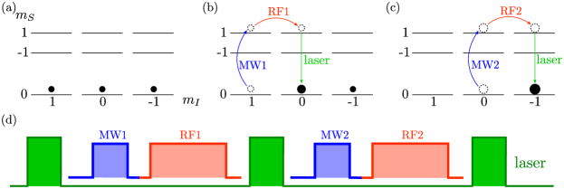
Figure 6: Scheme for nuclear spin initialization of the ¹⁴N nucleus. (a) Initially the population is distributed among the $m_{I}=0,\pm 1$. (b, c) With selective MW and RF pulses the population is first transferred from $m_{I}=+1$ to $m_{I}=0$ and then to $m_{I}=-1$ to initialize/polarize the nuclear spin. The laser is used to pump population in $m_{S}=1$ back to $m_{S}=0$. (d) Pulse protocol for the initialization process.

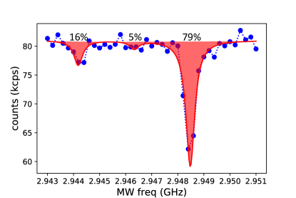
Figure 7: Nitrogen nuclear spin polarization. Results from an electron spin resonance (ESR) experiment performed immediately after the nuclear spin polarization protocol.

C.2 Lindbladian dissipation super-operator

As also described in the Appendix A of the main text, the interaction between the NV center and a green laser pulse can modeled as a POVM followed by a dissipation operator, and, overall, the dynamics of the open quantum system can be described by a master equation in Lindblad form. In this section, we will explicitly provide the expression of this Lindbladian dissipation operator.

For this purpose, from now on we will express operators in their matrix representation (with respect to the $S_{z}$-basis), such that

$$\ket{-1}\!\!\bra{-1}=\begin{pmatrix}0&0&0\\ 0&0&0\\ 0&0&1\end{pmatrix}\;;\;\ket{0}\!\!\bra{0}=\begin{pmatrix}0&0&0\\ 0&1&0\\ 0&0&0\end{pmatrix}\;;\;\ket{+1}\!\!\bra{+1}=\begin{pmatrix}1&0&0\\ 0&0&0\\ 0&0&0\end{pmatrix}.$$ (28)

In addition, we will use indistinguishably the term matrix or operator, unless otherwise specified, and we will adopt the formalism described in Ref. Havel (2003) for superoperators represented by $N^{2}\times N^{2}$ matrices, where $N=3$ is the dimension of the quantum system’s Hilbert space.

In this formalism, the Lindbladian dissipation super-operator (defined in Appendix A) is written as

$$\boldsymbol{\mathcal{L}}^{(t_{\mathrm{L}})}=\begin{pmatrix}e^{-t_{\mathrm{L}}\Gamma}&0&0&0&0&0&0&0&0\\ 0&e^{-t_{\mathrm{L}}\Gamma/2}&0&0&0&0&0&0&0\\ 0&0&e^{-t_{\mathrm{L}}\Gamma}&0&0&0&0&0&0\\ 0&0&0&e^{-t_{\mathrm{L}}\Gamma/2}&0&0&0&0&0\\ 1-e^{-t_{\mathrm{L}}\Gamma}&0&0&0&1&0&0&0&1-e^{-t_{\mathrm{L}}\Gamma}\\ 0&0&0&0&0&e^{-t_{\mathrm{L}}\Gamma/2}&0&0&0\\ 0&0&0&0&0&0&e^{-t_{\mathrm{L}}\Gamma}&0&0\\ 0&0&0&0&0&0&0&e^{-t_{\mathrm{L}}\Gamma/2}&0\\ 0&0&0&0&0&0&0&0&e^{-t_{\mathrm{L}}\Gamma}\end{pmatrix}$$ (29)

where $t_{\mathrm{L}}$ denotes the laser duration, and $\Gamma$ is an effective decay rate. Using laser pulses with $t_{\mathrm{L}}=41$ ns, we characterized that the effective decay rate equals $\Gamma\sim 12.2$ MHz.

C.3 Analytic $\gamma$ in the case of $\mathcal{H}=\mathcal{H}_{\mathrm{NV}}$

As explained in the main text, the effect of applying a single laser pulse can be described by the superoperator

$$\boldsymbol{\mathcal{A}}\equiv\sum_{j=1}^{4}\boldsymbol{\mathcal{D}}_{j}\boldsymbol{m}_{j}\,.$$ (30)

This superoperator can be computed explicitly from the definitions of $\boldsymbol{\mathcal{D}}_{j}$ and $\boldsymbol{m}_{j}$ [see also Appendix A in main text]. In this regard, by introducing the auxiliary matrices

$$\boldsymbol{A}_{1}\equiv\begin{pmatrix}1&0&0&0&0&0&0&0&0\\ 0&0&0&0&0&0&0&0&0\\ 0&0&0&0&0&0&0&0&0\\ 0&0&0&0&0&0&0&0&0\\ 0&0&0&0&1&0&0&0&0\\ 0&0&0&0&0&0&0&0&0\\ 0&0&0&0&0&0&0&0&0\\ 0&0&0&0&0&0&0&0&0\\ 0&0&0&0&0&0&0&0&1\end{pmatrix};\;\;\boldsymbol{A}_{2}\equiv\begin{pmatrix}0&0&0&0&0&0&0&0&0\\ 0&0&0&0&0&0&0&0&0\\ 0&0&0&0&0&0&0&0&0\\ 0&0&0&0&0&0&0&0&0\\ 1&0&0&0&1&0&0&0&1\\ 0&0&0&0&0&0&0&0&0\\ 0&0&0&0&0&0&0&0&0\\ 0&0&0&0&0&0&0&0&0\\ 0&0&0&0&0&0&0&0&0\end{pmatrix};\;\;\boldsymbol{A}_{3}\equiv\mathbb{1}_{9\times 9}-\boldsymbol{A}_{1}\,,$$

it holds that

$$\boldsymbol{\mathcal{A}}=\mu\boldsymbol{A}_{1}+(1-\mu)\boldsymbol{A}_{2}+\boldsymbol{A}_{3}(1-p_{\mathrm{abs}}),$$ (31)

where

$$\mu\equiv 1-(1-e^{-t_{\mathrm{L}}\Gamma})p_{\mathrm{abs}}\,.$$ (32)

It is no surprising that, if $p_{\mathrm{abs}}=0$, then $\boldsymbol{\mathcal{A}}_{(p_{\mathrm{abs}}=0)}=\mathbb{1}_{9\times 9}$. On the other hand, if $p_{\mathrm{abs}}=1$, then the POVM is actually a quantum projective measurement in the $S_{z}$-basis. This is the reason why $\boldsymbol{\mathcal{A}}_{(p_{\mathrm{abs}}=1)}=e^{-t_{\mathrm{L}}\Gamma}\boldsymbol{A}_{1}+(1-e^{-t_{\mathrm{L}}\Gamma})\boldsymbol{A}_{2}$ is practically equal to the Lindbladian dissipation super-operator $\boldsymbol{\mathcal{L}}$ [Eq. (29)], but without the terms involving coherences that is a signature of have applied a quantum projective measurement. Moreover, another special case occurs when $e^{-t_{\mathrm{L}}\Gamma}=1$, namely the case without dissipation, where Eq. (31) can be rewritten as $\boldsymbol{\mathcal{A}}=\boldsymbol{A}_{1}p_{\mathrm{abs}}+\mathbb{1}_{9\times 9}(1-p_{\mathrm{abs}})$ that identifies the mean effect of applying a quantum projective measurement of $S_{z}$ with probability $p_{\mathrm{abs}}$.

On the other hand, by taking $\mathcal{H}=\mathcal{H}_{\mathrm{NV}}$, the unitary evolution of the system is described by the following superoperator:

$$\boldsymbol{U}(\tau) \equiv\exp(-i\tau(\mathcal{H}\otimes\mathbb{1}_{3\times 3}-\mathbb{1}_{3\times 3}\otimes\mathcal{H}))$$

$$=\begin{pmatrix}1&0&0&0&0&0&0&0&0\\ 0&e_{+}&0&0&0&0&0&0&0\\ 0&0&\frac{e_{+}}{e_{-}}&0&0&0&0&0&0\\ 0&0&0&\frac{1}{e_{+}}&0&0&0&0&0\\ 0&0&0&0&1&0&0&0&0\\ 0&0&0&0&0&\frac{1}{e_{-}}&0&0&0\\ 0&0&0&0&0&0&\frac{e_{-}}{e_{+}}&0&0\\ 0&0&0&0&0&0&0&e_{-}&0\\ 0&0&0&0&0&0&0&0&1\end{pmatrix},$$

where $e_{\pm}\equiv e^{-i\tau E_{\pm 1}}$. Therefore, $\boldsymbol{\mathcal{B}}\equiv\boldsymbol{\mathcal{A}}\boldsymbol{U}$ can be written as

$$\boldsymbol{\mathcal{B}}=\mu\boldsymbol{A}_{1}+(1-\mu)\boldsymbol{A}_{2}+\boldsymbol{U}_{1}(\tau)(1-p_{\mathrm{abs}})$$ (33)

with $\boldsymbol{U}_{1}(\tau)\equiv\boldsymbol{U}(\tau)-\boldsymbol{A}_{1}$. Writing $\boldsymbol{\mathcal{B}}$ as in Eq. (33) is very useful, because the following properties hold:

$$\boldsymbol{A}_{i}^{2} =\boldsymbol{A}_{i}\;\;\mathrm{for}\;i\in\{1,2,3\}$$

$$\boldsymbol{A}_{1}\boldsymbol{A}_{3} =\boldsymbol{A}_{3}\boldsymbol{A}_{1}=\boldsymbol{A}_{2}\boldsymbol{A}_{3}=\boldsymbol{A}_{3}\boldsymbol{A}_{2}=\mathbb{0}_{9\times 9}$$

$$\boldsymbol{A}_{1}\boldsymbol{A}_{2} =\boldsymbol{A}_{2}\boldsymbol{A}_{1}=\boldsymbol{A}_{2}$$

$$(\boldsymbol{U}_{1}(\tau))^{n} =\boldsymbol{U}_{1}(n\tau)$$

$$\boldsymbol{A}_{i}\boldsymbol{U}_{1}(\tau) =\boldsymbol{U}_{1}(\tau)\boldsymbol{A}_{i}=\mathbb{0}_{9\times 9}\;\;\mathrm{for}\;i\in\{1,2\},$$

thus implying that

$$\boldsymbol{\mathcal{B}}^{N_{\mathrm{L}}}=\mu^{N_{\mathrm{L}}}\boldsymbol{A}_{1}+(1-\mu^{N_{\mathrm{L}}})\boldsymbol{A}_{2}+\boldsymbol{U}_{1}(N_{\mathrm{L}}\tau)(1-p_{\mathrm{abs}})^{N_{\mathrm{L}}}\,.$$ (34)

Moreover, being in the case of $\mathcal{H}=\mathcal{H}_{\mathrm{NV}}$, a thermal state $\rho^{\mathrm{th}}$ can be written according to the superoperators formalism Havel (2003) in the following way:

$$\operatorname{col}(\rho^{\mathrm{th}})=\frac{1}{Z}\operatorname{col}\left(\begin{bmatrix}e^{-\beta E_{+1}}&0&0\\ 0&1&0\\ 0&0&e^{-\beta E_{-1}}\end{bmatrix}\right)=\frac{1}{Z}\begin{pmatrix}e^{-\beta E_{+1}}\\ 0\\ 0\\ 0\\ 1\\ 0\\ 0\\ 0\\ e^{-\beta E_{-1}}\end{pmatrix}$$

where $Z\equiv\sum_{k=-1}^{1}e^{-\beta E_{i}}$. Hence, as final calculation, by exploiting that $\boldsymbol{A}_{1}^{\dagger}\operatorname{col}(\rho^{\mathrm{th}})=(\boldsymbol{U}_{1}(N_{\mathrm{L}}\tau))^{\dagger}\operatorname{col}(\rho^{\mathrm{th}})=\operatorname{col}(\rho^{\mathrm{th}})$, and $\boldsymbol{A}_{2}^{\dagger}\operatorname{col}(\rho^{\mathrm{th}})=\operatorname{col}(\mathbb{1}_{3\times 3})/Z$, the use of Eq. (34) allows us to obtain an analytic expression for $\gamma$, namely

$$\gamma =\operatorname{Tr}_{3\times 3}[(\boldsymbol{\mathcal{B}}^{\dagger})^{N_{\mathrm{L}}}\,\operatorname{col}[\rho^{\mathrm{th}}]]$$

$$=\mu^{N_{\mathrm{L}}}+\frac{3}{Z}(1-\mu^{N_{\mathrm{L}}})\,.$$ (35)

Let us observe that, apart the special cases mentioned before,

$$\lim_{N_{\mathrm{L}}\rightarrow\infty}\mu^{N_{\mathrm{L}}}=0\,,$$

meaning that

$$\lim_{N_{\mathrm{L}}\rightarrow\infty}\gamma=\frac{3}{Z}.$$ (36)

C.4 A method to extract $\eta^{*}$ from experimental data

Let us consider a 3LS initialized in the thermal state $\rho^{\mathrm{th}}\equiv\exp(-\beta H)/Z_{\beta}$ with $Z_{\beta}\equiv{\rm Tr}[\exp(-\beta H)]$. By diagonalizing the system Hamiltonian as $H=\sum_{i}E_{i}|E_{i}\rangle\!\langle E_{i}|$, the initial thermal initial state is equal to

$$\rho^{\mathrm{th}}=\sum_{i}\frac{e^{-\beta E_{i}}}{Z_{\beta}}|E_{i}\rangle\!\langle E_{i}|=\sum_{i}P_{i}|E_{i}\rangle\!\langle E_{i}|$$

where $P_{i}\equiv\exp(-\beta E_{i})/Z_{\beta}$.

Then, let us introduce the mean value of the exponentiated energy variation $\Delta E$, i.e.,

$$\langle\exp(-\eta\Delta E)\rangle=\sum_{i,j}P_{i}P_{j|i}e^{-\eta(E_{j}-E_{i})},$$ (37)

which strictly depends on the energy scaling factor $\eta$. Note that the average $\langle\exp(-\eta\Delta E)\rangle$ is defined by the sets $\{P_{i}\}$ and $\{P_{j|i}\}$, corresponding respectively to the probabilities to measure the initial energies of the system and the conditional probabilities to get $E_{j}$ at the end of the procedure after have measured $E_{i}$.

In the SSE regime, as described in the main text, the conditional probabilities $P_{j|i}$ does not depend upon the initially measured energies $E_{i}$. This entails that

$$P_{j|1}=P_{j|2}=P_{j|3}\equiv\widetilde{P}_{j}$$ (38)

for any $j$ such that

$$\langle\exp(-\eta\Delta E)\rangle=\sum_{i,j}P_{i}\widetilde{P}_{j}e^{-\eta(E_{j}-E_{i})}\,,$$ (39)

whereby the quantum state $\rho_{\rm fin}$ after the application of the 2nd energy projective measurement of the TPM measurement protocol is a mixed state, not necessarily thermal but completely described by the probabilities $\widetilde{P}_{j}$, namely

$$\rho_{\rm fin}=\sum_{j}\widetilde{P}_{j}|E_{j}\rangle\!\langle E_{j}|.$$

Now, to make our derivation compatible with the experimental setup and in particular with the case of $\mathcal{H}=\mathcal{H}_{\mathrm{mw}}$, we assume that the energy values are symmetric around zero, and, for the sake of brevity, we call $E_{1}=-\overline{E}$, $E_{2}=0$ and $E_{3}=\overline{E}$, with $\overline{E}$ constant value (in the experiment $\overline{E}=\hbar\omega/2$). In this way, by means of the substitution

$$x\equiv e^{\eta^{*}\overline{E}}\Longleftrightarrow\eta^{*}=\frac{1}{\overline{E}}\ln x\,,$$ (40)

the equation

$$\sum_{i,j}P_{i}\widetilde{P}_{j}e^{-\eta^{*}(E_{j}-E_{i})}=1$$

can be rewritten as the following polynomial equation:

$$(x-1)\left(P_{1}\widetilde{P}_{3}\,x^{3}+(P_{1}\widetilde{P}_{2}+P_{1}\widetilde{P}_{3}+P_{2}\widetilde{P}_{3})x^{2}-(P_{2}\widetilde{P}_{1}+P_{3}\widetilde{P}_{1}+P_{3}\widetilde{P}_{2})x-P_{3}\widetilde{P}_{1}\right)=0$$ (41)

Clearly, Eq. (41) contains the trivial solution $x=1$, i.e., $\eta^{*}=0$, while solving the third-order algebraic equation

$$P_{1}\widetilde{P}_{3}\,x^{3}+(P_{1}\widetilde{P}_{2}+P_{1}\widetilde{P}_{3}+P_{2}\widetilde{P}_{3})x^{2}-(P_{2}\widetilde{P}_{1}+P_{3}\widetilde{P}_{1}+P_{3}\widetilde{P}_{2})x=P_{3}\widetilde{P}_{1}$$ (42)

provides us the other value of $\eta^{*}\neq 0$ that obeys the fluctuation relation $\mathcal{G}(\eta^{*})=1$. In this regard, it is worth noting that, by applying the well-known Routh-Hurwitz criterion to the polynomial (42), we can also prove that just only root of Eq. (42) has positive real part. Indeed, according to the Routh-Hurwitz criterion, we recall that to each variation (permanence) of the sign of the coefficients of the first column of the Routh table corresponds to a root of the polynomial with a positive (negative) real part. In our case, there are always $2$ sign-permanences and only $1$ variation, for any possible value of the probabilities $P_{i}$ and $\widetilde{P}_{j}$. Being $\eta^{*}\propto\ln x$, only the unique solution $x\neq 0$ with positive real part is physical, thus providing us the (unique) non-trivial energy scaling factor $\eta^{*}$ such that $\mathcal{G}(\eta^{*})=1$.

Non-equilibrium steady-state condition fulfilled by $\eta^{*}$

Here, let us provide some more insights on the interpretation of $\eta^{*}$, and the condition that it has to fulfill by imposing the validity of the equality $\mathcal{G}(\eta^{*})=1$.

For this purpose, each probability $\widetilde{P}_{j}$ is decomposed in the product of two contributions: One is thermal and is associated to the inverse temperature $\beta_{\rm fin}$, while the other is a correction term that accounts for the (geometric) distance $\lambda$ concerning $\rho_{\rm fin}$ from being thermal Giachetti et al. (2020). Specifically, given the set $\{E_{j}\}$ of the system energies after the application of the measurement protocol, $\widetilde{P}_{j}$ can be written as

$$\widetilde{P}_{1}=\frac{e^{-\beta_{\rm fin}E_{1}}e^{\lambda(E_{2}-E_{3})^{2}}}{Z_{\beta_{\rm fin}}(\lambda)};\,\,\,\,\,\,\widetilde{P}_{2}=\frac{e^{-\beta_{\rm fin}E_{2}}e^{\lambda(E_{3}-E_{1})^{2}}}{Z_{\beta_{\rm fin}}(\lambda)};\,\,\,\,\,\,\widetilde{P}_{3}=\frac{e^{-\beta_{\rm fin}E_{3}}e^{\lambda(E_{1}-E_{2})^{2}}}{Z_{\beta_{\rm fin}}(\lambda)}\,,$$ (43)

where

$$Z_{\beta_{\rm fin}}(\lambda)=\exp(-\beta_{\rm fin}A+2\lambda B),\,\,\,\,\text{with}\,\,\,\,A=\sum_{j}E_{j}\,\,\,\,\text{and}\,\,\,\,B=\sum_{j}E_{j}^{2}-E_{1}E_{2}-E_{2}E_{3}-E_{3}E_{1},$$

denotes the corresponding discrete partition function. It is worth noting that the probabilities $\widetilde{P}_{1}$, $\widetilde{P}_{2}$ and $\widetilde{P}_{3}=1-\widetilde{P}_{1}-\widetilde{P}_{2}$ are written as a function of two free-parameters. Thus, known the energies $E_{j}$ and experimentally obtained the values of the probabilities $\widetilde{P}_{j}$ with $j=1,2,3$, $\beta_{\rm fin}$ and $\lambda$ can be derived by means of standard non-linear regression techniques.

Now, let us consider that $\mathcal{H}=\mathcal{H}_{\mathrm{mw}}$, which is the more involved one among the cases we have analyzed so far. In accordance with the experimental setup, the energies can be assumed symmetric around zero, as even shown above. In this way, by substituting the relations of Eq. (43) into Eq. (39) and imposing $\mathcal{G}(\eta^{*})=1$, after simple calculations we can end up in the following equality that corresponds to a non-equilibrium steady-state condition for the analysed open 3LS:

$$Z_{\beta}Z_{\beta_{\rm fin}}+C(\lambda)\left(3-Z_{\beta+\beta_{\rm fin}}\right)=C(\lambda)\left(Z_{(\beta-\beta_{\rm fin})-2\eta^{*}}+Z_{\beta_{\rm fin}+\eta^{*}}\right)+C(\lambda)^{4}Z_{\beta-\eta^{*}}$$ (44)

where

$$C(\lambda)=e^{\lambda\overline{E}^{2}};\,\,\,\,\,\,Z_{\beta-\eta^{*}}=\displaystyle{\sum_{k=-1}^{1}e^{-k\overline{E}(\beta-\eta^{*})}};$$

$$Z_{\beta_{\rm fin}+\eta^{*}}=\displaystyle{\sum_{k=-1}^{1}e^{-k\overline{E}(\beta_{\rm fin}+\eta^{*})}};\,\,\,\,\,\,Z_{(\beta-\beta_{\rm fin})-2\eta^{*}}=\displaystyle{\sum_{k=-1}^{1}e^{-k\overline{E}((\beta-\beta_{\rm fin})-2\eta^{*})}}.$$

Let us observe that $\eta^{*}=0$ is always solution of Eq. (44) for any value of $\lambda$, while for $\lambda=0$ the non-trivial solution $\eta^{*}$ of Eq. (44) is $\eta^{*}=\beta-\beta_{\rm fin}$ in perfect agreement with the Jarzynski-Wójcik relation Jarzynski and Wójcik (2004). Instead, for a value of $\lambda\neq 0$, Eq. (44) is numerically solved as a function of $\eta$, whereby the non-trivial solution $\eta^{*}$ is provided by the real and positive value of $\eta$ obeying the energy exchange fluctuation relation $\langle\exp(-\eta^{*}\Delta E)\rangle=1$.

References

- Maruyama et al. (2009) K. Maruyama, F. Nori, and V. Vedral, Rev. Mod. Phys. 81, 1 (2009).
- Bennett (1982) C. Bennett, Int. J. Theor. Phys. 21, 905 (1982).
- Funo et al. (2018) K. Funo, M. Ueda, and T. Sagawa, Thermodynamics in the quantum regime - Fundamental Aspects and New Directions (Springer International Publishing, 2018) pp. 249–273.
- Koski et al. (2014) J. V. Koski, V. F. Maisi, T. Sagawa, and J. P. Pekola, Phys. Rev. Lett. 113, 030601 (2014).
- Naghiloo et al. (2018) M. Naghiloo, J. J. Alonso, A. Romito, E. Lutz, and K. W. Murch, Phys. Rev. Lett. 121, 030604 (2018).
- Mandal and Jarzynski (2012) D. Mandal and C. Jarzynski, Proc. Nat. Acad. Sc. 109, 1 (2012).
- Kutvonen et al. (2016) A. Kutvonen, J. Koski, and T. Ala-Nissila, Scientific Reports , 1 (2016).
- Buffoni et al. (2019) L. Buffoni, A. Solfanelli, P. Verrucchi, A. Cuccoli, and M. Campisi, Phys. Rev. Lett. 122, 070603 (2019).
- Elouard et al. (2017a) C. Elouard, D. A. Herrera-Martí, M. Clusel, and A. Auffeves, npj Quantum Information 3 (2017a), 10.1038/s41534-017-0008-4.
- Gherardini et al. (2018) S. Gherardini, L. Buffoni, M. M. Müller, F. Caruso, M. Campisi, A. Trombettoni, and S. Ruffo, Phys. Rev. E 98, 032108 (2018).
- Toyabe et al. (2010) S. Toyabe, T. Sagawa, M. Ueda, E. Muneyuki, and M. Sano, Nat. Phys. 6, 988 (2010).
- Masuyama et al. (2018) Y. Masuyama, K. Funo, Y. Murashita, A. Noguchi, S. Kono, Y. Tabuchi, R. Yamazaki, M. Ueda, and Y. Nakamura, Nature Communications 9, 1291 (2018).
- Koski et al. (2015) J. V. Koski, A. Kutvonen, I. M. Khaymovich, T. Ala-Nissila, and J. P. Pekola, Phys. Rev. Lett. 115, 260602 (2015).
- Elouard et al. (2017b) C. Elouard, D. Herrera-Martí, B. Huard, and A. Auffèves, Phys. Rev. Lett. 118, 260603 (2017b).
- Campisi et al. (2017) M. Campisi, J. Pekola, and R. Fazio, New Journal of Physics 19, 053027 (2017).
- Schindler et al. (2011) P. Schindler, J. T. Barreiro, T. Monz, V. Nebendahl, D. Nigg, M. Chwalla, M. Hennrich, and R. Blatt, Science 332, 1059 (2011).
- Hirose and Cappellaro (2016) M. Hirose and P. Cappellaro, Nature 532, 77 (2016).
- Camati et al. (2016) P. A. Camati, J. P. S. Peterson, T. B. Batalhão, K. Micadei, A. M. Souza, R. S. Sarthour, I. S. Oliveira, and R. M. Serra, Phys. Rev. Lett. 117, 240502 (2016).
- Vidrighin et al. (2016) M. D. Vidrighin, O. Dahlsten, M. Barbieri, M. S. Kim, V. Vedral, and I. A. Walmsley, Phys. Rev. Lett. 116, 050401 (2016).
- Cottet et al. (2017) N. Cottet, S. Jezouin, L. Bretheau, P. Campagne-Ibarcq, Q. Ficheux, J. Anders, A. Auffèves, R. Azouit, P. Rouchon, and B. Huard, PNAS 114, 7561 (2017).
- Song et al. (2021) X. Song, M. Naghiloo, and K. Murch, Phys. Rev. A 104, 022211 (2021).
- Ji et al. (2022) W. Ji, Z. Chai, M. Wang, Y. Guo, X. Rong, F. Shi, C. Ren, Y. Wang, and J. Du, Phys. Rev. Lett. 128, 090602 (2022).
- Najera-Santos et al. (2020) B.-L. Najera-Santos, P. A. Camati, V. Métillon, M. Brune, J.-M. Raimond, A. Auffèves, and I. Dotsenko, Phys. Rev. Research 2, 032025 (2020).
- Verstraete et al. (2009) F. Verstraete, M. M. Wolf, and J. Ignacio Cirac, Nature Physics 5, 633 (2009).
- Pastawski et al. (2011) F. Pastawski, L. Clemente, and J. I. Cirac, Phys. Rev. A 83, 012304 (2011).
- Scarani et al. (2002) V. Scarani, M. Ziman, P. Štelmachovič, N. Gisin, and V. Bužek, Phys. Rev. Lett. 88, 097905 (2002).
- Nandkishore and Huse (2015) R. Nandkishore and D. A. Huse, Annual Review of Condensed Matter Physics 6, 15 (2015).
- Strasberg et al. (2017) P. Strasberg, G. Schaller, T. Brandes, and M. Esposito, Phys. Rev. X 7, 021003 (2017).
- Barreiro et al. (2011) J. T. Barreiro, M. Müller, P. Schindler, D. Nigg, T. Monz, M. Chwalla, M. Hennrich, C. F. Roos, P. Zoller, and R. Blatt, Nature 470, 486 (2011).
- Do et al. (2019) H.-V. Do, C. Lovecchio, I. Mastroserio, N. Fabbri, F. S. Cataliotti, S. Gherardini, M. M. Müller, N. Dalla Pozza, and F. Caruso, New Journal of Physics 21, 113056 (2019).
- Wolski et al. (2020) S. P. Wolski, D. Lachance-Quirion, Y. Tabuchi, S. Kono, A. Noguchi, K. Usami, and Y. Nakamura, Phys. Rev. Lett. 125, 117701 (2020).
- Xie et al. (2020) Y. Xie, J. Geng, H. Yu, X. Rong, Y. Wang, and J. Du, Phys. Rev. Applied 14, 014013 (2020).
- Lin et al. (2013) Y. Lin, J. P. Gaebler, F. Reiter, T. R. Tan, R. Bowler, A. S. Sørensen, D. Leibfried, and D. J. Wineland, Nature 504, 415 (2013).
- Barontini et al. (2015) G. Barontini, L. Hohmann, F. Haas, J. Estève, and J. Reichel, Science 349, 1317 (2015).
- Biella et al. (2017) A. Biella, F. Storme, J. Lebreuilly, D. Rossini, R. Fazio, I. Carusotto, and C. Ciuti, Phys. Rev. A 96, 023839 (2017).
- Lu et al. (2017) Y. Lu, S. Chakram, N. Leung, N. Earnest, R. K. Naik, Z. Huang, P. Groszkowski, E. Kapit, J. Koch, and D. I. Schuster, Phys. Rev. Lett. 119, 150502 (2017).
- Ma et al. (2019) R. Ma, B. Saxberg, C. Owens, N. Leung, Y. Lu, J. Simon, and D. I. Schuster, Nature 566, 51 (2019).
- Benatti and Floreanini (2003) F. Benatti and R. Floreanini, Irreversible quantum dynamics, Vol. 622 (Springer Science & Business Media, 2003).
- Dutta and Cooper (2021) S. Dutta and N. R. Cooper, Phys. Rev. Research 3, L012016 (2021).
- Gisin (1984) N. Gisin, Phys. Rev. Lett. 52, 1657 (1984).
- Jacobs (2014) K. Jacobs, Quantum measurement theory and its applications (Cambridge University Press, 2014).
- Esposito et al. (2009) M. Esposito, U. Harbola, and S. Mukamel, Rev. Mod. Phys. 81, 1665 (2009).
- Campisi et al. (2011) M. Campisi, P. Hänggi, and P. Talkner, Rev. Mod. Phys. 83, 771 (2011).
- An et al. (2015) S. An, J.-N. Zhang, M. Um, D. Lv, Y. Lu, J. Zhang, Z.-Q. Yin, H. T. Quan, and K. Kim, Nat. Phys. 11, 193 (2015).
- Smith et al. (2018) A. Smith, Y. Lu, S. An, X. Zhang, J.-N. Zhang, Z. Gong, H. T. Quan, C. Jarzynski, and K. Kim, New J. Phys. 20, 013008 (2018).
- Batalhão et al. (2014) T. B. Batalhão, A. M. Souza, L. Mazzola, R. Auccaise, R. S. Sarthour, I. S. Oliveira, J. Goold, G. De Chiara, M. Paternostro, and R. M. Serra, Phys. Rev. Lett. 113, 140601 (2014).
- Pal et al. (2019) S. Pal, T. S. Mahesh, and B. K. Agarwalla, Phys. Rev. A 100, 042119 (2019).
- Cerisola et al. (2017) F. Cerisola, Y. Margalit, S. Machluf, A. Roncaglia, J. Paz, and R. Folman, Nat. Comm. 8, 1241 (2017).
- Zhang et al. (2018) Z. Zhang, T. Wang, L. Xiang, Z. Jia, P. Duan, W. Cai, Z. Zhan, Z. Zong, J. Wu, L. Sun, Y. Yin, and G. Guo, New J. Phys. 20, 085001 (2018).
- Hernández-Gómez et al. (2020) S. Hernández-Gómez, S. Gherardini, F. Poggiali, F. S. Cataliotti, A. Trombettoni, P. Cappellaro, and N. Fabbri, Phys. Rev. Research 2, 023327 (2020).
- Ribeiro et al. (2020) P. H. S. Ribeiro, T. Häffner, G. L. Zanin, N. R. da Silva, R. M. de Araújo, W. C. Soares, R. J. de Assis, L. C. Céleri, and A. Forbes, Phys. Rev. A 101, 052113 (2020).
- Sagawa and Ueda (2008) T. Sagawa and M. Ueda, Phys. Rev. Lett. 100, 080403 (2008).
- Morikuni and Tasaki (2011) Y. Morikuni and H. Tasaki, Journal of Statistical Physics 143, 1 (2011).
- Funo et al. (2013) K. Funo, Y. Watanabe, and M. Ueda, Phys. Rev. E 88, 052121 (2013).
- Funo et al. (2015) K. Funo, Y. Murashita, and M. Ueda, New J. Phys. 17, 075005 (2015).
- Kafri and Deffner (2012) D. Kafri and S. Deffner, Phys. Rev. A 86, 044302 (2012).
- Rastegin (2013) A. E. Rastegin, J. Stat. Mech. 2013, P06016 (2013).
- Albash et al. (2013) T. Albash, D. A. Lidar, M. Marvian, and P. Zanardi, Phys. Rev. E 88, 032146 (2013).
- Goold et al. (2015) J. Goold, M. Paternostro, and K. Modi, Phys. Rev. Lett. 114, 060602 (2015).
- Havel (2003) T. F. Havel, Journal of Mathematical Physics 44, 534 (2003).
- Steiner et al. (2010) M. Steiner, P. Neumann, J. Beck, F. Jelezko, and J. Wrachtrup, Phys. Rev. B 81, 035205 (2010).
- Doherty et al. (2013) M. W. Doherty, N. B. Manson, P. Delaney, F. Jelezko, J. Wrachtrup, and L. C. L. Hollenberg, Phys. Rep. 528, 1 (2013).
- Wolters et al. (2013) J. Wolters, M. Strauß, R. S. Schoenfeld, and O. Benson, Phys. Rev. A 88, 020101 (2013).
- Talkner et al. (2007) P. Talkner, E. Lutz, and P. Hänggi, Phys. Rev. E 75, 050102 (2007).
- Rastegin and Życzkowski (2014) A. E. Rastegin and K. Życzkowski, Phys. Rev. E 89, 012127 (2014).
- Cimini et al. (2020) V. Cimini, S. Gherardini, M. Barbieri, I. Gianani, M. Sbroscia, L. Buffoni, M. Paternostro, and F. Caruso, npj Quantum Information 6, 96 (2020).
- Guarnieri et al. (2017) G. Guarnieri, S. Campbell, J. Goold, S. Pigeon, B. Vacchini, and M. Paternostro, New Journal of Physics 19, 103038 (2017).
- Gardas and Deffner (2015) B. Gardas and S. Deffner, Phys. Rev. E 92, 042126 (2015).
- Gherardini et al. (2021) S. Gherardini, A. Belenchia, M. Paternostro, and A. Trombettoni, Phys. Rev. A 104, L050203 (2021).
- Micadei et al. (2020) K. Micadei, G. T. Landi, and E. Lutz, Phys. Rev. Lett. 124, 090602 (2020).
- Sone et al. (2020) A. Sone, Y.-X. Liu, and P. Cappellaro, Phys. Rev. Lett. 125, 060602 (2020).
- Levy and Lostaglio (2020) A. Levy and M. Lostaglio, PRX Quantum 1, 010309 (2020).
- Roulet and Bruder (2018) A. Roulet and C. Bruder, Phys. Rev. Lett. 121, 063601 (2018).
- Abobeih et al. (2019) M. H. Abobeih, J. Randall, C. E. Bradley, H. P. Bartling, M. A. Bakker, M. J. Degen, M. Markham, D. J. Twitchen, and T. H. Taminiau, Nature 576, 411 (2019).
- Poggiali et al. (2017) F. Poggiali, P. Cappellaro, and N. Fabbri, Phys. Rev. B 95, 195308 (2017).
- Bar-Gill et al. (2013) N. Bar-Gill, L. M. Pham, A. Jarmola, D. Budker, and R. L. Walsworth, Nat. Commun. 4, 1743 (2013).
- Balasubramanian et al. (2009) G. Balasubramanian, P. Neumann, D. Twitchen, M. Markham, R. Kolesov, N. Mizuochi, J. Isoya, J. Achard, J. Beck, J. Tissler, V. Jacques, P. R. Hemmer, F. Jelezko, and J. Wrachtrup, Nature Materials 8, 383 (2009).
- Giachetti et al. (2020) G. Giachetti, S. Gherardini, A. Trombettoni, and S. Ruffo, Condensed Matter 5, 17 (2020).
- Jarzynski and Wójcik (2004) C. Jarzynski and D. K. Wójcik, Phys. Rev. Lett. 92, 230602 (2004).