1 Introduction

The recent measurement of the muon anomalous magnetic moment, $a_{\mu}\equiv(g_{\mu}-2)/2$, by the E989 experiment at Fermilab [1], in agreement with the previous BNL E821 result [2], implies a 4.2$\sigma$ discrepancy from the Standard Model (SM)

$$\Delta a_{\mu}\equiv a_{\mu}(\text{Exp})-a_{\mu}(\text{SM})=(251\pm 59)\times 10^{-11}\,,$$ (1.1)

following the Muon $g-2$ Theory Initiative recommended value for the SM theory prediction [3]. Although a recent lattice determination of the SM hadron vacuum polarization contribution to $a_{\mu}$ claims no sizeable deviation from the SM [4], we will work here under the hypothesis that $\Delta a_{\mu}$ is due to new physics. In particular, we will focus on the case in which new physics states are so heavy that their effects can be parameterized via the so-called SM Effective Field Theory (SMEFT) and ask the following question: What is the scale of new physics behind $\Delta a_{\mu}$?

This question is of practical relevance, given the futuristic possibility of resolving the new physics origin of $\Delta a_{\mu}$ via direct searches at high-energy particle colliders. As explored recently in [5, 6, 7], a muon collider seems to be the best option for this goal. However, while the very existence of the SMEFT operators contributing to $\Delta a_{\mu}$ could be tested via processes like $\mu^{+}\mu^{-}\to Z(\gamma)h$ or $\mu^{+}\mu^{-}\to t\overline{t}$ at a multi-TeV-scale muon collider [6], it is less clear whether the origin of the muon $g-2$ SMEFT operators can be resolved via the direct production of new on-shell states responsible for $\Delta a_{\mu}$. This is the question that we want to address in the present work, using the tools of perturbative unitarity. Unitarity bounds on the new physics interpretation of $\Delta a_{\mu}$ were previously considered in [5, 7] focusing however on a specific class of renormalizable models. Here, we will consider instead the most conservative case in which unitarity limits are obtained within the SMEFT and reach a more pessimistic conclusion about the possibility of establishing a no-lose theorem for testing the origin of $\Delta a_{\mu}$ at a future high-energy particle collider.

Generally speaking, given a low-energy determination of an EFT coefficient, unitarity methods can be used either within an EFT approach, in order to infer an upper bound on the scale of new physics unitarizing EFT scattering amplitudes, or within explicit new physics (renormalizable) models. In the latter case, one obtains a perturbativity bound on certain renormalizable couplings that can be translated into an upper bound on the mass of new on-shell degrees of freedom. In the present work we will be interested in both these approaches. First, we will consider a SMEFT analysis in which $\Delta a_{\mu}$ is explained in terms of a set of Wilson coefficients normalized to some cut-off scale², $C_{i}/\Lambda^{2}$, and later deal with renormalizable models featuring new heavy mediators that can be matched onto the SMEFT. Schematically,

$$\Delta a_{\mu}\sim\frac{C_{i}}{\Lambda^{2}}=\frac{\text{(loops)}\times\text{(couplings)}}{M^{2}_{\rm on-shell}}\,,$$ (1.2)

where $M_{\rm on-shell}$ denote the mass of new on-shell states and we included possible loop factors in the matching between the new physics model and the SMEFT operators. Hence, by fixing the value of the SMEFT coefficients $C_{i}/\Lambda^{2}$ in terms of $\Delta a_{\mu}$, we will consider high-energy scatterings sourced by the associated effective operators, determine the $\sqrt{s}$ that saturates perturbative unitarity (according to a standard criterium to be specified in Sect. 2) and interpret the latter as an upper bound on the scale of new physics responsible for the muon $g-2$ anomaly. Analogously, in the case of new physics models, we will use the unitarity tool in order to set perturbativity bounds on the new physics couplings and in turn (given Eq. (1.2)) an upper limit on $M_{\rm on-shell}$. While the first approach is model-independent (barring possible degeneracies in the choice of the effective operators) and yields the most conservative bound on the scale of new physics, the second approach relies on further assumptions, but it directly connects to new on-shell degrees of freedom which are the prime targets of direct searches at high-energy particle colliders.

The paper is structured as follows. We start in Sect. 2 with a brief review of partial wave unitarity, in order to set notations and clarify the physical interpretation of unitarity bounds. Next, we consider unitarity bounds within a SMEFT approach (Sect. 3) and within renormalizable models matching onto the SMEFT operators (Sect. 4). Finally, we comment in Sect. 5 on non-renormalizable realizations which can saturate the unitarity bounds obtained in the SMEFT. Our main findings and implications for the direct resolution of the muon $g-2$ anomaly at high-energy particle colliders are summarized in the conclusions (Sect. 6). Technical aspects of partial wave unitarity calculations, both in the SMEFT and in renormalizable setups, are deferred to Apps. A–B.

2 Partial wave unitarity

We start with an instant review of partial wave unitarity, which will serve to set notations and discuss the physical significance of unitarity bounds.

The key point of our analysis is the study of scattering amplitudes with fixed total angular momentum $J$, the so-called partial waves. Here we focus only on the case of $2\to 2$ partial waves (while the $2\to 3$ scattering is discussed in App. A.2) defined as

$$a^{J}_{fi}=\frac{1}{32\pi}\int_{-1}^{1}\mathrm{d}\cos\theta\,d^{J}_{\mu_{i}\mu_{f}}(\theta)\,\mathcal{T}_{fi}(\sqrt{s},\cos\theta)\,,$$ (2.1)

with $\theta$ the scattering angle in the centre-of-mass frame, $(2\pi)^{4}\delta^{(4)}(P_{i}-P_{f})i\mathcal{T}_{fi}(\sqrt{s},\cos\theta)=\bra{f}S-1\ket{i}$ and $S$ the $S$-matrix. Here, $d^{J}_{\mu_{i}\mu_{f}}$ is Wigner’s $d$-function that arises in the construction of the two-particle incoming (outcoming) state of helicities $\mu_{i}$ ($\mu_{f}$) onto angular momentum $J$ [8]. The $S$-matrix unitarity condition $S^{\dagger}S=1$ then yields the relation

$$\frac{1}{2i}(a^{J}_{fi}-a^{J^{*}}_{if})=\sum_{h}a^{J^{*}}_{hf}a^{J}_{hi}\qquad\Longrightarrow\qquad\mbox{Im}\,(a_{ii}^{J})=\sum_{h}|a^{J}_{hi}|^{2}\geq|a^{J}_{ii}|^{2}\,,$$ (2.2)

where we have restricted ourselves to the elastic channel $h=i=f$. The equation on the right hand side of (2.2) defines a circle in the complex plane inside which the amplitude must lie at all orders,

$$\Big{(}\mbox{Re}\,a^{J}_{ii}\Big{)}^{2}+\Big{(}\mbox{Im}\,a^{J}_{ii}-\frac{1}{2}\Big{)}^{2}\leq\frac{1}{4}\,,$$ (2.3)

suggesting the following bound, under the assumption of real tree-level amplitudes:

$$|\mbox{Re}\,a^{J}_{ii}|\leq\frac{1}{2}\,.$$ (2.4)

Hence, in order to extract the bound, one needs to fully diagonalize the matrix $a^{J}$. Once this is achieved, every eigenvalue will give an independent constraint. In the presence of multiple scattering channels, it follows from Eq. (2.4) that the strongest bound arises from the largest eigenvalue of $a^{J}$. When the latter bound is saturated, it basically means that one needs a correction of at least $40$% from higher orders to get back inside the unitarity circle, thus signaling the breakdown of perturbation theory (see e.g. [9, 10]). Here, $a^{J}$ stands for the leading order expansion of the partial wave, both in the coupling constants and in external momenta over cut-off scale for the case of an EFT.

Although the criterium is somewhat arbitrary, and hence Eq. (2.4) should not be understood as a strict bound, we stick to that for historical reasons [11]. Strictly speaking, a violation of the perturbative unitarity criterium in Eq. (2.4) should be conservatively interpreted as the onset of a regime of incalculability due to the breakdown of the perturbative expansion either in couplings or external momenta. More specifically, in the case of an EFT (where scattering amplitudes grow with energy) the scale of unitarity violation, hereafter denoted as

$$\sqrt{s}=\Lambda_{U}\qquad\Longrightarrow\qquad|\mbox{Re}\,a^{J}_{ii}|=\frac{1}{2}\,,$$ (2.5)

can be associated with the onset of “new physics”, where on-shell new degrees of freedom should manifest themselves and be kinematically accessible. Although one can conceive exotic UV completions where this is not the case [12], well-known physical systems behave in this way. Unitarity methods can be employed in renormalizable setups as well. In this case, the unitarity limit corresponds to the failure of the coupling expansion and hence the bound on the renormalizable coupling can be understood as a perturbativity constraint.

3 SMEFT

In this section we present the unitarity bounds for the new physics interpretation of the muon $g-2$ anomaly within a SMEFT approach. The strategy consists in fixing the Wilson coefficients ($C_{i}/\Lambda^{2}$) in terms of the observable $\Delta a_{\mu}$ and determine next the energy scale $\sqrt{s}$ that saturates the unitarity bounds derived from the tree-level scattering amplitudes sourced by the effective operator. The shorthand $1/\Lambda_{i}^{2}\equiv C_{i}/\Lambda^{2}$ is understood in the following.

3.1 SMEFT approach to $\Delta a_{\mu}$

Assuming a short-distance new physics origin of $\Delta a_{\mu}$, the leading SMEFT operators contributing up to one-loop order are (see Refs. [6, 13] for a more systematic discussion)

$$\mathscr{L}_{g-2}^{\rm SMEFT} =\frac{C^{\ell}_{eB}}{\Lambda^{2}}(\overline{\ell}_{L}\sigma^{\mu\nu}e_{R})HB_{\mu\nu}+\frac{C^{\ell}_{eW}}{\Lambda^{2}}(\overline{\ell}_{L}\sigma^{\mu\nu}e_{R})\tau^{I}HW^{I}_{\mu\nu}$$

$$+\frac{C^{\ell q}_{T}}{\Lambda^{2}}(\overline{\ell}^{a}_{L}\sigma_{\mu\nu}e_{R})\varepsilon_{ab}(\overline{Q}^{b}_{L}\sigma^{\mu\nu}u_{R})+\text{h.c.}\,,$$ (3.1)

which results in [6]

$$\Delta a_{\ell}\simeq\frac{4m_{\ell}v}{e\sqrt{2}\Lambda^{2}}\left(\mbox{Re}\,C^{\ell}_{e\gamma}-\frac{3\alpha}{2\pi}\frac{c^{2}_{W}-s^{2}_{W}}{s_{W}c_{W}}\mbox{Re}\,C^{\ell}_{eZ}\log\frac{\Lambda}{m_{Z}}\right)-\sum_{q=t,c,u}\frac{4m_{\ell}m_{q}}{\pi^{2}}\frac{\mbox{Re}\,C^{\ell q}_{T}}{\Lambda^{2}}\log\frac{\Lambda}{m_{q}}\,,$$ (3.2)

where $C_{e\gamma}=c_{W}C_{eB}-s_{W}C_{eW}$ and $C_{eZ}=-s_{W}C_{eB}-c_{W}C_{eW}$, in terms of the weak mixing angle. For the Wilson coefficients of the dipole operators that contribute at tree level to $\Delta a_{\ell}$, one can consistently include one-loop running, obtaining [14, 15]

$$C^{\ell}_{e\gamma}(m_{\ell})\simeq C^{\ell}_{e\gamma}(\Lambda)\left(1-\frac{3y^{2}_{t}}{16\pi^{2}}\log\frac{\Lambda}{m_{t}}-\frac{4\alpha}{\pi}\log\frac{\Lambda}{m_{\ell}}\right)\,.$$ (3.3)

A convenient numerical parameterization reads

$$\Delta a_{\mu}\simeq 2.5\times 10^{-9}\left(\frac{277\ \text{TeV}}{\Lambda}\right)^{2}\left(\mbox{Re}\,C^{\mu}_{e\gamma}(\Lambda)-0.28\,\mbox{Re}\,C^{\mu t}_{T}(\Lambda)-0.047\,\mbox{Re}\,C^{\mu}_{eZ}(\Lambda)\right)\,,$$ (3.4)

where we have kept only the leading top-quark contribution for $C_{T}$ (since we are interested on scenarios which maximize the scale of new physics) and the logs have been evaluated for $\Lambda=277$ TeV. Note, however, that the full log dependence will be retained in the numerical analysis below. In the following, we will drop the scale dependence of the Wilson coefficients, which are understood to be evaluated at the scale $\Lambda$.

3.2 Unitarity bounds

Given Eq. (3.1), we can compute the scale of unitarity violation $\Lambda_{U}$ (defined via Eq. (2.5)) associated with each of the dimension-6 operators involved. To do so, we consider here only $2\to 2$ scattering processes, since the $2\to 3$ processes (mediated by $\mathcal{O}_{eW}$) turn out to be suppressed by the weak gauge coupling and the 3-particle phase space, as shown in Appendix A.2. The results obtained by switching one operator per time are collected in Table 1, where the bound in correspondence of different initial and final states ($i\neq f$) comes from the diagonalization of the scattering matrix (cf. discussion below Eq. (2.4)). In App. A we present the full calculation of the unitarity bounds stemming from the ${\rm SU}(2)_{L}$ dipole operator, which presents several non-trivial aspects, like the presence of higher than $J=0$ partial waves, the multiplicity in ${\rm SU}(2)_{L}$ space and the possibility of $2\to 3$ scatterings.

Operator	$\Lambda_{U}$	$i\to f$ Channels	$J$
$\frac{1}{\Lambda^{2}_{eB}}(\overline{\ell}_{L}\sigma^{\mu\nu}e_{R})HB_{\mu\nu}$	$2\sqrt{\pi}|\Lambda_{eB}|$	$Be_{R}\to H^{\dagger}\ell_{L}$	$1/2$
$\frac{1}{\Lambda^{2}_{eW}}(\overline{\ell}_{L}\sigma^{\mu\nu}e_{R})\tau^{I}HW^{I}_{\mu\nu}$	$2\sqrt{\pi}\left(\frac{2}{3}\right)^{1/4}|\Lambda_{eW}|$	$W\overline{\ell}_{L}\to H^{\dagger}\overline{e}_{R}$	$1/2$
$\frac{1}{\Lambda^{2}_{T,\ell}}(\overline{\ell}^{a}_{L}\sigma_{\mu\nu}e_{R})\varepsilon_{ab}(\overline{Q}^{b}_{L}\sigma^{\mu\nu}u_{R})$	$2\sqrt{\frac{\pi}{3\sqrt{2}}}|\Lambda_{T,\ell}|$	$e_{R}u_{R}\to Q_{L}\ell_{L}$	$0$

Table 1: Unitarity violation scale for the SMEFT operators contributing to $\Delta a_{\mu}$.

We next make contact with the physical observable $\Delta a_{\mu}$, whose dependence from the Wilson coefficients can be read off Eq. (3.4). Turning on one operator per time, we find the following numerical values for the unitarity violation scales:

• $\mathcal{O}^{\mu}_{eB}\equiv(\overline{\ell}_{L}\sigma^{\mu\nu}e_{R})HB_{\mu\nu}$

  $$\Lambda_{U}\simeq 277\ \text{TeV}\ 2\sqrt{\pi}\sqrt{c_{W}+0.047s_{W}}\simeq 930\ \text{TeV}\,.$$ (3.5)

• $\mathcal{O}^{\mu}_{eW}\equiv(\overline{\ell}_{L}\sigma^{\mu\nu}e_{R})\tau^{I}HW^{I}_{\mu\nu}$

  $$\Lambda_{U}\simeq 277\ \text{TeV}\ 2\sqrt{\pi}\left(\frac{2}{3}\right)^{1/4}\sqrt{s_{W}-0.047c_{W}}\simeq 590\ \text{TeV}\,.$$ (3.6)

• $\mathcal{O}^{\mu t}_{T}\equiv(\overline{\ell}^{a}_{L}\sigma_{\mu\nu}e_{R})\varepsilon_{ab}(\overline{Q}^{b}_{L}\sigma^{\mu\nu}u_{R})$

  $$\Lambda_{U}\simeq 277\ \text{TeV}\ 2\sqrt{\frac{\pi}{3\sqrt{2}}}\sqrt{0.28}\simeq 240\ \text{TeV}\,.$$ (3.7)

Hence, the scale of new physics is maximized if the origin of $\Delta a_{\mu}$ stems from a dipole operator oriented in the ${\rm U}(1)_{Y}$ direction.

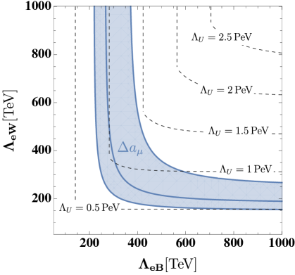
Figure 1: In blue, the region in the ($\Lambda_{eB}$, $\Lambda_{eW}$) plane that is needed to reproduce the experimental value of $\Delta a_{\mu}$ at the $2\sigma$ level (with the central line corresponding to the central value of $\Delta a_{\mu}$). The dashed iso-lines represent the unitarity bound $\Lambda_{U}$, defined according to Eq. (A.13).

If more than one operator is switched on, correlations can arise between the Wilson coefficients whenever they couple same sectors of the theory. For instance, in the case in which both the dipole operators $\mathcal{O}^{\mu}_{eW}$ and $\mathcal{O}^{\mu}_{eB}$ are present one can derive a combined bound (see Eq. (A.13)) which leads to the region displayed in Fig. 1. Note that for $\Lambda_{eB}\to\infty$ ($\Lambda_{eW}\to\infty$) we reproduce the bound with $\mathcal{O}^{\mu}_{eW}$ ($\mathcal{O}^{\mu}_{eB}$) only. However, if both operators contribute sizeably to $\Delta a_{\mu}$, the unitarity bound can be slightly relaxed above the PeV scale.

4 Renormalizable models

We next consider simplified models featuring new heavy states, which after being integrated out match onto the dipole and tensor SMEFT operators contributing to $\Delta a_{\mu}$ (cf. Eq. (3.4)). We will then use unitarity methods to set perturbativity limits on renormalizable couplings and in turn set an upper bound on the mass of the new on-shell physics states. To maximize the scale of new physics, we will focus on two renormalizable setups based scalar-fermion Yukawa theories, allowing for a left-right chirality flip that is either entirely due to new physics (Sect. 4.1) or with a top Yukawa insertion (Sect. 4.2).

4.1 One-loop matching onto the dipole operator

In order to match onto the dipole operator at one loop we consider a simplified model with a new complex scalar $S=(1,1,Y+1)$ and two vector-like fermions $F_{\ell}=(1,2,Y+\frac{1}{2})$ and $F_{e}=(1,1,Y)$ allowing for a mixing via the SM Higgs (see e.g. [16, 17, 5, 7])

$$\mathscr{L}^{g-2}_{\rm FFS} =\lambda_{L}\overline{F}_{\ell}\ell_{L}S+\lambda_{R}\overline{F}_{e}e_{R}S+\overline{F}_{\ell}(y_{L}P_{L}+y_{R}P_{R})F_{e}H+\rm{h.c.}$$

$$-M_{\ell}\overline{F}_{\ell}F_{\ell}-M_{e}\overline{F}_{e}F_{e}-m_{S}^{2}|S|^{2}-\kappa\,|H|^{2}\,|S|^{2}-\lambda_{S}|S|^{4}\,.$$ (4.1)

The FFS model allows for a chirality flip of the external leptons via the product of couplings $\lambda^{*}_{L}y_{L,R}\lambda_{R}$ (cf. Fig. 2), which can be used to maximize the scale of new physics. For $vy_{L,R}\ll M_{\ell},M_{e},m_{S}$, we can integrate out the new physics states and find at one loop

$$\dfrac{C^{\mu}_{e\gamma}}{\Lambda^{2}} =-\dfrac{e\lambda_{L}^{*}\lambda_{R}}{32\pi^{2}m_{S}^{2}}\dfrac{\sqrt{x_{\ell}x_{e}}}{(x_{\ell}-x_{e})}\,\Bigg{\{}Q_{S}\left[y_{R}\left(g_{S}(x_{\ell})-g_{S}(x_{e})\right)+y_{L}\left(\sqrt{\dfrac{x_{\ell}}{x_{e}}}g_{S}(x_{\ell})-\sqrt{\dfrac{x_{e}}{x_{\ell}}}g_{S}(x_{e})\right)\right]$$

$$+Q_{F}\left[y_{R}\left(g_{F}(x_{\ell})-g_{F}(x_{e})\right)+y_{L}\left(\sqrt{\dfrac{x_{\ell}}{x_{e}}}g_{F}(x_{\ell})-\sqrt{\dfrac{x_{e}}{x_{\ell}}}g_{F}(x_{e})\right)\right]\Bigg{\}}\,,$$ (4.2)

where $Q_{S}=Y+1$, $Q_{F}=Y$, $x_{\ell,e}=M^{2}_{\ell,e}/m^{2}_{S}$ and the loop functions are given by

$$g_{F}(x)=\dfrac{x^{2}-4x+3+2\log x}{2(x-1)^{3}}\,,\qquad g_{S}(x)=\frac{x^{2}-2x\log x-1}{2(x-1)^{3}}\,.$$ (4.3)

This result agrees with Ref. [18] in which the special case $y_{L}=y_{R}$ was considered. Note that in Eq. (4.1) we already matched onto the photon dipole operator at the scale $\Lambda$, while the connection with the low-energy observable $\Delta a_{\mu}$ is given in Eq. (3.4).

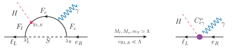
Figure 2: Sample diagram of the FFS model matching onto $C^{\mu}_{e\gamma}$ at the scale $\Lambda$.

Our goal is to maximize the mass of the lightest new physics state for a fixed value of the Wilson coefficient. This is achieved in the degenerate limit $m_{S}=M_{\ell}=M_{e}$, yielding

$$\dfrac{C^{\mu}_{e\gamma}}{\Lambda^{2}}=-\dfrac{e\lambda_{L}^{*}\lambda_{R}}{384\pi^{2}m_{S}^{2}}\left[\left(1+2Y\right)y_{L}-\left(1+4Y\right)y_{R}\right]\,\simeq\dfrac{eY\lambda_{L}^{*}\lambda_{R}}{192\pi^{2}m_{S}^{2}}\left(2y_{R}-y_{L}\right)\,,$$ (4.4)

where in the last expression we took $Y\gg 1$.

The unitarity bounds for the FFS model are summarized in Table 2, where in the case of multiple scattering channels the bound corresponds to the highest eigenvalue of $a^{J}$. We refer to App. B for further details on their derivation. Applying these bounds, the maximum value of the combination $|\mbox{Re}\,(\lambda_{L}^{*}\lambda_{R}(2y_{R}-y_{L}))|$ entering Eq. (4.4) is $\approx 121$, while $|eY|\lesssim 3.5$. Hence, we obtain

$$\Delta a_{\mu}\simeq 2.5\times 10^{-9}\left(\frac{131\ \text{TeV}}{m_{S}}\right)^{2}\left(\dfrac{eY}{3.5}\right)\left(\dfrac{\mbox{Re}\,\left(\lambda_{L}^{*}\lambda_{R}(2y_{R}-y_{L})\right)}{121}\right)\,,$$ (4.5)

which shows that the $\Delta a_{\mu}$ explanation in the FFS model requires an upper bound on the mass of the new on-shell states of about 130 TeV. On the other hand, due to the extra loop suppression, it is not possible to saturate the unitarity bound that was obtained within the SMEFT (see Eq. (3.5)).

Unitarity bound	$i\to f$ Channels	$J$
$\left|\mbox{Re}\,(\lambda_{L}^{*}\lambda_{R})\right|<8\pi$	$e_{R}F_{\ell_{R}}\to e_{R}F_{\ell_{R}}$	$0$
$\left|\mbox{Re}\,(y_{L}^{*}y_{R})\right|<{8\pi}/{\sqrt{2}}$	$F_{e_{R}}\overline{F}_{e_{L}}\to F_{e_{R}}\overline{F}_{e_{L}}$	$0$
$\left|\mbox{Re}\,(y_{L}^{*}y_{R})\pm\sqrt{4|\lambda_{L}|^{2}|\lambda_{R}|^{2}+(y_{L}^{*})^{2}y_{R}^{2}}\right|<16\pi$	$i,f=F_{\ell_{R}}\overline{F}_{e_{L}},e_{R}\overline{\ell}_{L}$	$0$
$2|\lambda_{L}|^{2}+|\lambda_{R}|^{2}<8\pi$	$i,f=F_{\ell_{R}}\overline{\ell}_{L},F_{e_{L}}\overline{e}_{R}$	$0$
$|y_{R}|<\sqrt{8\pi}$	$HF_{\ell_{L}}\to HF_{\ell_{L}}$	$1/2$
$|\lambda_{R}|^{2}+2|y_{L}|^{2}<16\pi$	$i,f=Se_{R},H^{\dagger}F_{\ell,R}$	$1/2$
$\left|\mbox{Re}\,(y_{L}\lambda_{L}^{*})\right|<{8\pi}/{\sqrt{2}}$	$i,f=F_{e_{R}}S^{\dagger},e_{R}H$	$1/2$
$|\lambda_{R}|^{2}+\sqrt{32|y_{L}|^{2}|\lambda_{R}|^{2}+|\lambda_{R}|^{4}}<32\pi$	$i,f=S\overline{F}_{e_{L}},H^{\dagger}\ell_{L}$	$1/2$
$\left|\mbox{Re}\,(\lambda_{L}y_{L})\right|<{16\pi}/{\sqrt{2}}$	$\ell_{L}\overline{F}_{e_{L}}\to SH^{\dagger}$	$1$
$\left|\mbox{Re}\,(y_{L}^{*}\lambda_{R})\right|<{16\pi}/{\sqrt{2}}$	$F_{\ell_{R}}\overline{e}_{R}\to HS$	$1$
$|\kappa|<{8\pi}/{\sqrt{2}}$	$HH^{\dagger}\to SS^{\dagger}$	$0$
$|g_{Y}(Y+1)|<\sqrt{6\pi}$	$SB_{\mu}\to SB_{\mu}$	$1/2$

Table 2: Unitarity bounds for the FFS model.

4.2 Tree-level matching onto the tensor operator

We now consider a simplified model that matches onto the tensor operator $\mathcal{O}^{\mu q}_{T}$. The scalar leptoquarks $R_{2}=(3,2,\tfrac{7}{6})$ and $S_{1}=(3,1,-\tfrac{1}{3})$ allow for a coupling to the top-quark with both chiralities (see e.g. [19]), thus maximizing the effect on $\Delta a_{\mu}$ via a top-mass insertion. Massive vectors can also lead to renormalizable extensions, but they result at least into a $m_{b}/m_{t}$ suppression compared to scalar extensions (see e.g. [20]).

Let us focus for definiteness on the $R_{2}$ case (similar conclusions apply to $S_{1}$). The relevant interaction Lagrangian reads

$$\mathscr{L}^{g-2}_{R_{2}}\supset\lambda_{L}\,\overline{t}_{R}\ell_{L}^{a}\,\varepsilon_{ab}R_{2}^{b}+\lambda_{R}\,\overline{q}_{L}^{a}\,\mu_{R}R_{2a}+\text{h.c.}$$ (4.6)

where $a$ and $b$ are ${\rm SU}(2)_{L}$ indices and $\varepsilon=i\sigma_{2}$. Upon integrating out the leptoquark with mass $m_{R_{2}}\gg v$ (cf. Fig. 3), one obtains [21, 13]

$$\dfrac{C^{\mu t}_{T}}{\Lambda^{2}}=-\dfrac{\lambda^{*}_{L}\lambda_{R}}{8m_{R_{2}}^{2}}\,.$$ (4.7)

The unitarity bounds for the $R_{2}$ model (see App. B for details) are collected in Table 3 and they imply $|\mbox{Re}\,(\lambda^{*}_{L}\lambda_{R})|\lesssim 12$. Hence, we can recast the contribution to $\Delta a_{\mu}$ via Eq. (3.4) as

$$\Delta a_{\mu}\simeq 2.5\times 10^{-9}\left(\frac{180\ \text{TeV}}{m_{R_{2}}}\right)^{2}\left(\dfrac{\mbox{Re}\,(\lambda^{*}_{L}\lambda_{R})}{12}\right)\,.$$ (4.8)

Hence, we conclude that in the leptoquark model one expects $m_{R_{2}}\lesssim 180\ \text{TeV}$ (the same numerical result is obtained for $S_{1}$), thus providing the largest new physics scale among the renormalizable extensions responsible for $\Delta a_{\mu}$. Moreover, since the matching with the tensor operator is at tree level, the leptoquark model fairly reproduces the unitarity bound from the SMEFT operator (see Eq. (3.7)).

Figure 3: Sample diagram of the leptoquark model matching onto $C^{\mu t}_{T}$ at the scale $\Lambda$.

Unitarity bound	$i\to f$ Channels	$J$
$|\lambda_{L}|^{2}+|\lambda_{R}|^{2}<8\pi$	$i,f=t_{R}\overline{\ell}_{L},q_{L}\overline{\mu}_{R}$	$0$
$\left|\mbox{Re}\,(\lambda_{R}\lambda_{L}^{*})\right|<{8\pi}/{\sqrt{3}}$	$\mu_{R}\overline{\ell}_{L}\to q_{L}\overline{t}_{R}$	$0$
$|\lambda_{R}|^{2}<{8\pi}/{3}$	$q_{L}R_{2}^{*}\to q_{L}R_{2}^{*}$	$1/2$
$|\lambda_{L}|^{2}<{16\pi}/{3}$	$t_{R}R_{2}^{*}\to t_{R}R_{2}^{*}$	$1/2$

Table 3: Unitarity bounds for the couplings of the leptoquark model defined in Eq. (4.6).

4.3 Raising the scale of new physics via multiplicity?

Naively, one could be tempted to increase the upper limit on the scale of new physics by adding ${\cal N}$ copies of new physics states contributing to $\Delta a_{\mu}$. However, while both $C_{e\gamma}$ and $C_{T}$ increase by a factor of ${\cal N}$, the unitarity bounds on the couplings gets also stronger due to the correlation of the scattering channels, so that larger new physics scales cannot be reached.

In order to see this, consider e.g. the FFS model with ${\cal N}$ copies of $F_{\ell}$, $F_{e}$ and $S$. The scaling of the unitarity bounds is most easily seen in processes where the SM states are exchanged in the $s$-channel, for example $S^{i}F_{\ell_{R}}^{i}\to S^{j}F_{\ell_{R}}^{j}$. Since $\ell_{L}$ is coupled to all copies in the same way, the $\mathcal{T}$-matrix can be written as

$$\mathcal{T}^{J=1/2}=\frac{1}{32\pi}|\lambda_{L}|^{2}J_{\cal N}\,,$$ (4.9)

where $J_{\cal N}$ is a ${\cal N}\times{\cal N}$ matrix filled with 1. Given that the largest eigenvalue of $J_{\cal N}$ is ${\cal N}$, the unitarity bound on $\lambda_{L}$ reads

$$|\lambda_{L}|<\sqrt{\frac{16\pi}{{\cal N}}}\,.$$ (4.10)

Similar processes can be considered for all the couplings in Eq. (4.1), leading to a $1/\sqrt{{\cal N}}$ scaling for each Yukawa coupling. Hence, the overall ${\cal N}$ contribution to $\Delta a_{\mu}\propto{\cal N}\,\mbox{Re}\,(\lambda_{L}^{*}\lambda_{R}y_{L,R})/m^{2}_{S}$ is compensated by the $1/\sqrt{{\cal N}}$ scaling of the unitarity bounds on the couplings and, for fixed $\Delta a_{\mu}$, the mass of extra states gets even lowered at large ${\cal N}$. In this respect, we reach a different conclusion from the analysis in Ref. [7].

The same considerations apply if we consider just one new scalar and ${\cal N}$ new fermions. The situation is different with ${\cal N}$ scalars and just one family of fermions, since $S$ does not couple directly to the Higgs (barring the portal coupling $\kappa$ in Eq. (4.1), which however does not contribute to $\Delta a_{\mu}$). This implies that only $\lambda_{L}$ and $\lambda_{R}$ will scale as $1/\sqrt{{\cal N}}$, which in turn means that $\Delta a_{\mu}$ does not change. Similar arguments apply when considering larger ${\rm SU}(2)_{L}$ representations, thus implying that the minimal choice we made for the FFS model ensures that $m_{S}$ is maximized. The case of the leptoquark $R_{2}$ is analogous to what we have just described for ${\cal N}$ new scalars, with the new fermions of the FFS model replaced by SM fields. Given that $\lambda_{L}$ and $\lambda_{R}$ would scale as $1/\sqrt{{\cal N}}$, there is no gain in taking ${\cal N}$ copies of leptoquarks.

5 Non-renormalizable models

Till now we focused on renormalizable extensions of the SM addressing $\Delta a_{\mu}$ and showed that they predict on-shell new physics states well below the unitarity bound obtained from the SMEFT dipole operators, suggesting instead that new physics can hide up to the PeV scale. Nonetheless, the SMEFT bound should be understood as the most conservative one and applies if the origin of $\Delta a_{\mu}$ can be for instance traced back to a strongly-coupled dynamics. While such a scenario could have calculability issues, we want to provide here an intermediate step in which the SMEFT dipole operators are generated via a tree-level exchange of a new vector resonance from a strongly-coupled sector taking inspiration from the case of the $\rho$ meson in QCD, but whose UV origin we leave unspecified.

Spin-1 vector resonances are conveniently described via the two-index anti-symmetric tensor field ${\cal V}_{\mu\nu}$, following the formalism of Ref. [22]. In particular, we consider a composite spin-1 state featuring the same gauge quantum numbers of the SM Higgs doublet and described via the effective Lagrangian

$$\mathcal{L}_{{\cal V}} =-{\cal D}^{\mu}{\cal V}_{\mu\nu}^{\dagger}{\cal D}_{\rho}{\cal V}^{\rho\nu}+\dfrac{1}{2}m^{2}_{{\cal V}}{\cal V}_{\mu\nu}^{\dagger}{\cal V}^{\mu\nu}$$

$$+c_{HB}{\cal V}_{\mu\nu}^{\dagger}HB^{\mu\nu}+{c}_{HW}{\cal V}_{\mu\nu}^{\dagger}\tau^{I}HW^{I,\mu\nu}+c_{\ell e}{\cal V}_{\mu\nu}(\overline{\ell}_{L}\sigma^{\mu\nu}e_{R})+\ldots\,,$$ (5.1)

where we neglected ${\cal V}_{\mu\nu}$ self-interactions as well as other higher-dimensional operators. In fact, Eq. (5) should be understood as the leading term of an effective non-renormalizable Lagrangian, with cut-off scale $\Lambda_{{\cal V}}$ above $m_{{\cal V}}$. The free Lagrangian of Eq. (5) propagates three degrees of freedom describing a free spin-1 particle of mass $m_{{\cal V}}$, with propagator [22, 23, 24]

$$i\Delta_{\mu\nu;\rho\sigma}(q) =\frac{2i}{m^{2}_{\cal V}-q^{2}}\left[{\cal I}_{\mu\nu;\rho\sigma}(q)-\dfrac{q^{2}}{m^{2}_{\cal V}}{\cal P}_{\mu\nu;\rho\sigma}(q)\right]\,,$$ (5.2)

where ${\cal I}_{\mu\nu;\rho\sigma}=\left(g_{\mu\rho}g_{\nu\sigma}-g_{\mu\sigma}g_{\nu\rho}\right)/2$ and ${\cal P}^{\mu\nu;\rho\sigma}=\left(P_{T}^{\mu\rho}P_{T}^{\nu\sigma}-P_{T}^{\mu\sigma}P_{T}^{\nu\rho}\right)/2$ with $P_{T}^{\mu\nu}=g^{\mu\nu}-q^{\mu}q^{\nu}/q^{2}$. Assuming that there is a calculable regime where one can parametrically keep $m_{{\cal V}}\lesssim\Lambda_{{\cal V}}$ (in analogy to the chiral approach to the $\rho$ meson in QCD, for which $m_{\rho}\lesssim\Lambda_{\chi}\sim 1$ GeV) we can integrate ${\cal V}_{\mu\nu}$ out and get the following tree-level matching contribution with the photon dipole operator (cf. also Fig. 4)

$$\frac{C^{\mu}_{e\gamma}}{\Lambda^{2}}=-\frac{2\left(c_{W}c_{HB}-s_{W}{c}_{HW}\right)c_{\ell e}}{m^{2}_{\cal V}}\,.$$ (5.3)

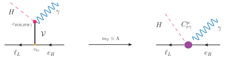
Figure 4: Tree-level matching onto the photon dipole operator via the exchange of a spin-1 vector resonance.

Hence, we obtain

$$\Delta a_{\mu}\simeq 2.5\times 10^{-9}\left(\frac{1\ \text{PeV}}{m_{\cal V}}\right)^{2}\left(\frac{\mbox{Re}\,\left(\left(-c_{W}c_{HB}+s_{W}{c}_{HW}\right)c_{\ell e}\right)}{7.5}\right)\,,$$ (5.4)

where we normalized $m_{\cal V}$ at the PeV scale, that is in the ballpark of the unitarity bound obtained from the SMEFT dipole operators. It should be noted that although the operators in the second line of Eq. (5) have canonical dimension equal to 4, scattering amplitudes involving the $c_{HB,HW,\ell e}$ couplings, as e.g. $HB\to e_{R}\overline{\ell}_{L}$, grow like $s/m^{2}_{\cal V}$ due to the high-energy behaviour of the propagator in Eq. (5.2). Hence, the effective description of the vector resonance breaks down not far above $m_{\cal V}$, being the theory non-renormalizable.

6 Conclusions

Unitarity bounds are a useful tool in order to infer the regime of validity of a given physical description. In EFT approaches, the energy scale at which unitarity is violated in tree-level scattering amplitudes can be often associated to the onset of the new physics completing the effective description. Instead, within renormalizable setups unitarity bounds are a synonym of perturbativity bounds on the size of the adimensional couplings. In this work we have investigated unitarity constraints on the new physics interpretation of the muon $g-2$ anomaly. Assuming a short-distance SMEFT origin of the latter, we have first computed unitarity bounds considering a set of leading (dipole and tensor) operators contributing to $\Delta a_{\mu}$. It turns out that the scale of tree-level unitarity violation is maximized in the case of dipole operators and reaches the PeV scale when both ${\rm U}(1)_{Y}$ and ${\rm SU}(2)_{L}$ dipoles are switched on (cf. Fig. 1). Hence, most conservatively, in order to resolve the new physics origin of the SMEFT operators behind $\Delta a_{\mu}$ one would need to probe high-energy scales up to the PeV. This most pessimistic scenario, clearly outside from the direct reach of next-generation high-energy particle colliders, can be understood as a no-lose theorem for the muon $g-2$ puzzle. Of course, the new physics origin of $\Delta a_{\mu}$ might reside well below the PeV scale, as it is indeed suggested by simplified models based on renormalizable scalar-Yukawa theories. In the latter case we have considered a couple of well-known scenarios matching either on the tensor (at tree level) or the dipole (at one loop) operators of the SMEFT analysis. In both cases, we have computed unitarity bounds on renormalizable couplings, thus allowing the mass of the new on-shell states to be maximized. The latter are found to be $M_{\rm on-shell}\lesssim 130$ TeV and $\lesssim 180$ TeV, respectively for the dipole and the tensor operators. Moreover, we have shown that multiplicity does not help to relax those bound because unitarity limits scale as well with the number of species.

Since the bound obtained within renormalizable models is well below the SMEFT bound, it is fair to ask which UV completions could lead to a new physics resolution of the muon $g-2$ puzzle hidden at the PeV scale. In fact, one could imagine a strongly-coupled dynamics at the PeV scale that is equivalent to writing the SMEFT Lagrangian. Here, we have provided instead an intermediate step in which the SMEFT dipole operators are generated via the tree-level exchange of a new spin-1 vector resonance described by a two-index anti-symmetric tensor field ${\cal V}_{\mu\nu}$ with the same quantum numbers of the SM Higgs and whose origin should be traced back to the dynamics of a strongly-coupled sector. This effective scenario provides a non-trivial example in which the dipole effective operators are generated via tree-level matching, thus suggesting that the SMEFT unitarity bound can be saturated with new on-shell states hidden at the PeV scale. It would be interesting to investigate whether a UV dynamics leading to such effective scenario can be explicitly realized.

Appendix A Unitarity bounds in the SMEFT

In this Appendix we expand on some aspects of the calculation of unitarity bounds in the SMEFT. The case of the operator $\mathcal{O}_{eW}=(\overline{\ell}_{L}\sigma^{\mu\nu}e_{R})\tau^{I}HW^{I}_{\mu\nu}$ is analyzed in detail, since it offers the possibility of discussing several non-trivial aspects, like the multiplicity of the scattering amplitude in ${\rm SU}(2)_{L}$ space, the contribution of higher-partial waves and that of $2\to 3$ scatterings. The calculations of the unitarity bounds for $\mathcal{O}_{eB}$ and $\mathcal{O}_{T}$ follow in close analogy and are not reported here.

A.1 $2\to 2$ scattering

Consider the $2\to 2$ scattering $W^{I}\overline{\ell}_{L}^{a}\to H^{\dagger,b}\overline{e}_{R}$ sourced by $\mathcal{O}_{eW}$, where we have explicitly written the ${\rm SU}(2)_{L}$ indices ($I=1,2,3$ in the adjoint and $a,b=1,2$ in the fundamental). Taking a $W$ with positive helicity, the lowest partial wave is $J=1/2$. The only possible source for a multiplicity of states in this sector is given by ${\rm SU}(2)_{L}$, giving a total of $3\times 2+2=8$ states, so the $J=1/2$ sector is a $8\times 8$ matrix, with entries given by $(\tau^{I})^{ab}$. Ordering the states as $\{W^{1}\overline{\ell}_{L}^{1},W^{1}\overline{\ell}_{L}^{2},W^{2}\overline{\ell}_{L}^{1},W^{2}\overline{\ell}_{L}^{2},W^{3}\overline{\ell}_{L}^{1},W^{3}\overline{\ell}_{L}^{2},H^{\dagger,1}\overline{e}_{R},H^{\dagger,2}\overline{e}_{R}\}$, we have

$$a^{J=1/2}_{fi}=a_{1/2}\begin{pmatrix}0&0&0&\tau^{1}\\ 0&0&0&\tau^{2}\\ 0&0&0&\tau^{3}\\ \tau^{1}&\tau^{2}&\tau^{3}&0\end{pmatrix}\,,$$ (A.1)

where $a_{1/2}=\frac{\sqrt{2}}{16\pi}\frac{s}{\Lambda^{2}_{eW}}$ encodes the result of Eq. (2.1) (and whose calculation is reported below). The largest eigenvalue of this matrix is $a^{J=1/2}_{ii}=\sqrt{3}a_{1/2}$, leading to the bound

$$\sqrt{s}<\Lambda_{U}=2\sqrt{\pi}\left(\frac{2}{3}\right)^{1/4}|\Lambda_{eW}|\,.$$ (A.2)

We now report the computation of the amplitude $a_{1/2}$ of Eq. (A.1). The process is

$$W(p,+)+\overline{\ell}_{L}(k)\to H(p^{\prime})+\overline{e}_{R}(k^{\prime})\,,$$ (A.3)

with $\vec{p}$ chosen along the $\hat{z}$ direction and the scattering angle $\theta$ the one formed by $\vec{p}$ and $\vec{p}^{\prime}$, and we have suppressed ${\rm SU}(2)_{L}$ indices. The $\mathcal{T}$-matrix element is

$$\mathcal{T}_{fi}=\frac{1}{\Lambda^{2}_{eW}}(p_{\mu}\varepsilon_{\nu}^{(+)}(\vec{p})-p_{\nu}\varepsilon_{\mu}^{(+)}(\vec{p}))({\overline{v}}^{(R)}(\vec{k})\sigma^{\mu\nu}v^{(L)}(\vec{k}^{\prime}))=2\sqrt{2}\frac{s}{\Lambda^{2}_{eW}}\cos\frac{\theta}{2}\,.$$ (A.4)

Since the lowest partial wave is $J=1/2$, and $\mu_{i}=\mu_{f}=1/2$, we need the $d$-function $d^{1/2}_{1/2,1/2}(\theta)=\cos\frac{\theta}{2}$. Plugging this into Eq. (2.1) gives

$$a_{1/2}=\frac{1}{32\pi}2\sqrt{2}\frac{s}{\Lambda^{2}_{eW}}\int_{-1}^{1}\mathrm{d}\cos\theta\cos^{2}\frac{\theta}{2}=\frac{\sqrt{2}}{16\pi}\frac{s}{\Lambda^{2}_{eW}}\,.$$ (A.5)

A.2 $2\to 3$ scattering

Here we show how the unitarity bound for the $2\to 3$ scattering is weaker than the one obtained for $2\to 2$ processes, in the special case of the operator $\mathcal{O}_{eW}$. This is due to the presence of the weak gauge coupling $g_{2}\simeq 0.6$, in addition to the phase-space suppression of the 3-particle final state. Extracting the $2\to 3$ partial wave is slightly more involved, since one needs to construct the three-particle states at fixed total $J$, which in the centre-of-mass frame have five degrees of freedom we have to integrate over, instead of the only two polar angles of the two-particle case. In particular, a convenient set of variables is the one obtained by combining 2 particles together (as it is done e.g. for semi-leptonic hadron decays, in which one usually considers the lepton pair). Fixing their mass $m_{R}^{2}$, and boosting to the frame in which these are back-to back, one can construct a state with fixed $J_{R}$ (and helicity $\lambda_{R}$) out of the two-particles, and then combine this with the third to form the eigenstates of the total angular momentum $J$. The explicit expression is given by

$$\ket{\sqrt{s},m_{R}^{2};JM;\vec{\lambda}} =N_{J}^{(3)}(\vec{\lambda})\sum_{J_{R},\lambda_{R}}\int\mathrm{d}\Omega_{1}\mathrm{d}\Omega_{R}\mathcal{D}^{J^{*}}_{M,\lambda_{R}-\lambda_{3}}(\phi_{R},\theta_{R},-\phi_{R})$$

$$\times\mathcal{D}^{J_{R}^{*}}_{\lambda_{R},\lambda_{1}-\lambda_{2}}(\phi_{1},\theta_{1},-\phi_{1})\ket{\sqrt{s},m_{R}^{2};\theta_{R}\phi_{R};\theta_{1}\phi_{1};\vec{\lambda}}\,,$$ (A.6)

where $\mathcal{D}_{MM^{\prime}}(\alpha,\beta,\gamma)$ are Wigner’s $\mathcal{D}$-matrices, with $\alpha$, $\beta$, $\gamma$ Euler angles in the $z$-$y$-$z$ convention and

$$N_{J}^{(3)}(\vec{\lambda})=\frac{\sqrt{2J+1}}{4\pi}\left(\sum_{J_{R},\lambda_{R}}\frac{1}{2J_{R}+1}\right)^{-1/2}$$ (A.7)

is a normalisation factor, the angles $\theta_{1}$ and $\phi_{1}$ are the polar angles of particle 1 in the centre-of-mass of particles 1 and 2, $\theta_{R}$ and $\phi_{R}$ the polar angles of $\vec{p}_{1}+\vec{p}_{2}$ in the centre-of-mass of the three particles (i.e. $\vec{p}_{1}+\vec{p}_{2}+\vec{p}_{3}=0$), and $\vec{\lambda}=(\lambda_{1},\lambda_{2},\lambda_{3})$ are the helicities. The dependence on $\vec{\lambda}$ in the normalization factor is implicit, since the helicities determine over which values the sum over $J_{R}$, $\lambda_{R}$ runs. This will have to be considered case by case, depending on the type of particles involved and the partial wave one wants to obtain. With these states, we can extract the $2\to 3$ partial wave at fixed $m_{R}^{2}$, in the case of massless particles, as follows:

$$a^{J}_{fi} =\frac{\sqrt{s-m_{R}^{2}}}{256\pi^{2}\sqrt{s}}\left(\sum_{J_{R}}\frac{1}{2J_{R}+1}\right)^{-1/2}\sum_{J_{R}}\int\mathrm{d}\cos{\theta_{1}}\mathrm{d}\cos{\theta_{R}}$$

$$\times d^{J}_{\mu_{i},\mu_{i}}(\theta_{R})d^{J_{R}}_{\mu_{i}+\lambda_{3},\lambda_{1}-\lambda_{2}}(\theta_{1})\mathcal{M}_{fi}(\sqrt{s},m_{R}^{2};\theta_{1},\theta_{R};r,s,\vec{\lambda})\,,$$ (A.8)

where $r,s$ are the helicities of the incoming particles, and $\mu_{i}$ is their sum. The largest eigenvalue is then given by

$$\xi=\sqrt{\int_{0}^{s}\mathrm{d}m_{R}^{2}\left[a^{J}_{fi}(2\to 3;m_{R}^{2})\right]^{2}}\,.$$ (A.9)

Finally, the full diagonalisation of the $\mathcal{T}$-matrix is then achieved by considering the multiplicities in helicity and gauge space, which can lead to further enhancements.

In the case of the operator $\mathcal{O}_{eW}$, the largest channel is the $J=1/2$ scattering $He_{R}\to\ell_{L}WW$, yielding the bound

$$\sqrt{s}<\Lambda_{U}^{2\to 3}=\frac{32\pi}{\sqrt{g_{2}}}\sqrt{\frac{1}{8+\pi^{2}}\frac{1}{\sqrt{3}}}\,\Lambda_{eW}\,.$$ (A.10)

Comparing this with the $2\to 2$ bound in Eq. (A.2), $\Lambda_{U}^{2\to 2}=2\sqrt{\pi}\Lambda_{eW}$, one finds

$$\frac{\Lambda_{U}^{2\to 2}}{\Lambda_{U}^{2\to 3}}\simeq 0.3\sqrt{g_{2}}\,.$$ (A.11)

A.3 A combined bound with $\mathcal{O}_{eW}$ and $\mathcal{O}_{eB}$

Let us examine now the case in which both the operators $\mathcal{O}_{eW}$ and $\mathcal{O}_{eB}$ are switched on. Consider again the scattering $W\overline{\ell}_{L}\to H^{\dagger}\overline{e}_{R}$ mediated by $\mathcal{O}_{eW}$. From the point of view of SM gauge symmetry, the final state forces the process to occur in the (1,2,1/2) representation. The same applies to the process $B\overline{\ell}_{L}\to H^{\dagger}\overline{e}_{R}$. We can therefore construct the $\mathcal{T}$-matrix in a similar manner as above. Now ordering the states as $\{W\overline{\ell}_{L},B\overline{\ell}_{L},H^{\dagger}e_{R}\}$, we find

$$a^{J=1/2}_{fi}=\tilde{a}_{1/2}\begin{pmatrix}0&0&\frac{1}{\Lambda^{2}_{eW}}A\\ 0&0&\frac{1}{\Lambda^{2}_{eB}}\mathbf{1}_{2\times 2}\\ \frac{1}{\Lambda^{2}_{eW}}A^{\dagger}&\frac{1}{\Lambda^{2}_{eB}}\mathbf{1}_{2\times 2}&0\end{pmatrix}\qquad A=\begin{pmatrix}\tau^{1}\\ \tau^{2}\\ \tau^{3}\end{pmatrix}\,,$$ (A.12)

with $\tilde{a}_{1/2}=\frac{s\sqrt{2}}{16\pi}$. The largest eigenvalue is $a^{J=1/2}_{ii}=\tilde{a}_{1/2}\sqrt{\frac{3}{\Lambda^{4}_{eW}}+\frac{1}{\Lambda^{4}_{eB}}}$, thus we find

$$\sqrt{s}<\Lambda_{U}=\text{min}\left[2\sqrt{\sqrt{2}\pi}\left(\frac{3}{\Lambda^{4}_{eW}}+\frac{1}{\Lambda^{4}_{eB}}\right)^{-1/4},\ 2\sqrt{\pi}|\Lambda_{eB}|\right]\,.$$ (A.13)

Hence, as shown in Fig. 1, we can constrain simultaneously $C_{eB}$ and $C_{eW}$. It is worth noticing that, following the same procedure with the scattering $Be_{R}\to H^{\dagger}\ell_{L}$ (which minimizes the bound for $\mathcal{O}_{eB}$), i.e. considering also $We_{R}\to H^{\dagger}\ell_{L}$, we would still find two independent bounds for the two operators. This is due to the fact that the state $We_{R}$ transforms as $(1,3,-1)$, which cannot mix into the ${\rm SU}(2)_{L}$ singlet configuration formed by $Be_{R}$.

Appendix B Unitarity bounds in renormalizable models

In this section we provide some details about the computation of the unitarity bounds for the simplified models of Sect. 4. Staring from the case of the $R_{2}$ leptoquark, whose interactions relevant for the anomalous magnetic moment are described by the lagrangian (4.6),

$$\mathscr{L}^{g-2}_{R_{2}}\supset\lambda_{L}\,\overline{t}_{R}\ell_{L}^{a}\,\varepsilon_{ab}R_{2}^{b}+\lambda_{R}\,\overline{q}_{L}^{a}\,\mu_{R}R_{2a}+\text{h.c.}\,,$$ (B.1)

one can see that several $2\to 2$ scattering processes can be considered, both scalar and fermion mediated. The goal is therefore to analyse all of them, in order to identify which channel gives the strongest bound. In general, since there is more than one coupling (two in this case), the different channels will yield independent (combined in general) bounds, as in Table 3. The overall bound on the couplings $\lambda_{L}$ and $\lambda_{R}$ can then be visualised as the region defined by the intersection of all the individual constraints. In particular, if the interest lies in one specific combination of said couplings, as for example in Eq. (4.7), one can maximise the function over this region.

The best way to proceed in order to compute the unitarity bounds is to classify the possible scattering sectors according to their quantum numbers under the SM gauge symmetry, exploiting the fact that different sectors cannot mix due to gauge invariance. As an example, we show here how the bound is obtained when the leptoquark $R_{2}$ is exchanged in the $s$-channel, i.e. the gauge quantum numbers are $(3,2,\frac{7}{6})$. The lowest partial wave, giving the strongest bound, is $J=0$ in this case, and the $\mathcal{T}$-matrix takes the form

$$\mathcal{T}^{J=0}_{(3,2,7/6)}=\frac{1}{16\pi}\begin{pmatrix}|\lambda_{L}|^{2}&\lambda_{L}^{*}\lambda_{R}^{*}\\ \lambda_{L}\lambda_{R}&|\lambda_{R}|^{2}\end{pmatrix}\,,$$ (B.2)

where we have ordered the incoming and outgoing states as $\{t_{R}\overline{\ell}_{L},q_{L}\overline{\mu}_{R}\}$ and we have taken the high-energy limit. Diagonalising, the unitarity bound for the highest eigenvalue reads

$$|\lambda_{L}|^{2}+|\lambda_{R}|^{2}<8\pi\,.$$ (B.3)

All other bounds in Table 3 are obtained in a similar way.

The case of the simplified models with one extra scalar and two extra fermions (FFS) is very similar to the case just described, with some complication due to the presence of more fields and couplings, which increases the number of channels one needs to consider. The philosophy, however, is the same: consider all possible processes and identify the strongest independent bounds (the results are in Table 2). Once this is done, one can extract a bound on the specific combination of the couplings entering the formula for $\Delta a_{\mu}$. Finally, the bounds on the parameter $Y$ entering the hypercharges of the fields $F_{e}$, $F_{\ell}$ and $S$ have been obtained by considering scattering channels that are completely separated from the ones where the new Yukawa couplings are involved, i.e. considering initial and final states containing the $B$ boson. This has the twofold advantage of giving an independent bound on $Y$ while also avoiding issues of unphysical singularities arising in the exchange of a massless vector boson.

References

- [1] Muon g-2 Collaboration, B. Abi et al., “Measurement of the Positive Muon Anomalous Magnetic Moment to 0.46 ppm,” Phys. Rev. Lett. 126 no. 14, (2021) 141801, arXiv:2104.03281 [hep-ex].
- [2] Muon g-2 Collaboration, G. W. Bennett et al., “Final Report of the Muon E821 Anomalous Magnetic Moment Measurement at BNL,” Phys. Rev. D 73 (2006) 072003, arXiv:hep-ex/0602035.
- [3] T. Aoyama et al., “The anomalous magnetic moment of the muon in the Standard Model,” Phys. Rept. 887 (2020) 1–166, arXiv:2006.04822 [hep-ph].
- [4] S. Borsanyi et al., “Leading hadronic contribution to the muon 2 magnetic moment from lattice QCD,” arXiv:2002.12347 [hep-lat].
- [5] R. Capdevilla, D. Curtin, Y. Kahn, and G. Krnjaic, “A Guaranteed Discovery at Future Muon Colliders,” Phys. Rev. D 103 no. 7, (2021) 075028, arXiv:2006.16277 [hep-ph].
- [6] D. Buttazzo and P. Paradisi, “Probing the muon g-2 anomaly at a Muon Collider,” arXiv:2012.02769 [hep-ph].
- [7] R. Capdevilla, D. Curtin, Y. Kahn, and G. Krnjaic, “A No-Lose Theorem for Discovering the New Physics of at Muon Colliders,” arXiv:2101.10334 [hep-ph].
- [8] M. Jacob and G. C. Wick, “On the General Theory of Collisions for Particles with Spin,” Annals Phys. 7 (1959) 404–428.
- [9] L. Di Luzio, J. F. Kamenik, and M. Nardecchia, “Implications of perturbative unitarity for scalar di-boson resonance searches at LHC,” Eur. Phys. J. C 77 no. 1, (2017) 30, arXiv:1604.05746 [hep-ph].
- [10] L. Di Luzio and M. Nardecchia, “What is the scale of new physics behind the -flavour anomalies?,” Eur. Phys. J. C 77 no. 8, (2017) 536, arXiv:1706.01868 [hep-ph].
- [11] B. W. Lee, C. Quigg, and H. B. Thacker, “Weak Interactions at Very High-Energies: The Role of the Higgs Boson Mass,” Phys. Rev. D 16 (1977) 1519.
- [12] G. Dvali, G. F. Giudice, C. Gomez, and A. Kehagias, “UV-Completion by Classicalization,” JHEP 08 (2011) 108, arXiv:1010.1415 [hep-ph].
- [13] J. Aebischer, W. Dekens, E. E. Jenkins, A. V. Manohar, D. Sengupta, and P. Stoffer, “Effective field theory interpretation of lepton magnetic and electric dipole moments,” arXiv:2102.08954 [hep-ph].
- [14] G. Degrassi and G. F. Giudice, “QED logarithms in the electroweak corrections to the muon anomalous magnetic moment,” Phys. Rev. D 58 (1998) 053007, arXiv:hep-ph/9803384.
- [15] R. Alonso, E. E. Jenkins, A. V. Manohar, and M. Trott, “Renormalization Group Evolution of the Standard Model Dimension Six Operators III: Gauge Coupling Dependence and Phenomenology,” JHEP 04 (2014) 159, arXiv:1312.2014 [hep-ph].
- [16] L. Calibbi, R. Ziegler, and J. Zupan, “Minimal models for dark matter and the muon g2 anomaly,” JHEP 07 (2018) 046, arXiv:1804.00009 [hep-ph].
- [17] P. Arnan, A. Crivellin, M. Fedele, and F. Mescia, “Generic Loop Effects of New Scalars and Fermions in , and a Vector-like Generation,” JHEP 06 (2019) 118, arXiv:1904.05890 [hep-ph].
- [18] A. Crivellin and M. Hoferichter, “Consequences of chirally enhanced explanations of for and ,” arXiv:2104.03202 [hep-ph].
- [19] I. Doršner, S. Fajfer, A. Greljo, J. F. Kamenik, and N. Košnik, “Physics of leptoquarks in precision experiments and at particle colliders,” Phys. Rept. 641 (2016) 1–68, arXiv:1603.04993 [hep-ph].
- [20] C. Biggio, M. Bordone, L. Di Luzio, and G. Ridolfi, “Massive vectors and loop observables: the case,” JHEP 10 (2016) 002, arXiv:1607.07621 [hep-ph].
- [21] F. Feruglio, P. Paradisi, and O. Sumensari, “Implications of scalar and tensor explanations of ,” JHEP 11 (2018) 191, arXiv:1806.10155 [hep-ph].
- [22] G. Ecker, J. Gasser, A. Pich, and E. de Rafael, “The Role of Resonances in Chiral Perturbation Theory,” Nucl. Phys. B 321 (1989) 311–342.
- [23] O. Catà, “Lurking pseudovectors below the TeV scale,” Eur. Phys. J. C 74 no. 8, (2014) 2991, arXiv:1402.4990 [hep-ph].
- [24] A. Pich, I. Rosell, J. Santos, and J. J. Sanz-Cillero, “Fingerprints of heavy scales in electroweak effective Lagrangians,” JHEP 04 (2017) 012, arXiv:1609.06659 [hep-ph].
- [25] J. de Blas, J. C. Criado, M. Perez-Victoria, and J. Santiago, “Effective description of general extensions of the Standard Model: the complete tree-level dictionary,” JHEP 03 (2018) 109, arXiv:1711.10391 [hep-ph].