Relation Matters in Sampling: A Scalable Multi-Relational Graph Neural Network for Drug-Drug Interaction Prediction

Abstract

Sampling is an established technique to scale graph neural networks to large graphs. Current approaches however assume the graphs to be homogeneous in terms of relations and ignore relation types, critically important in biomedical graphs. Multi-relational graphs contain various types of relations that usually come with variable frequency and have different importance for the problem at hand. We propose an approach to modeling the importance of relation types for neighborhood sampling in graph neural networks and show that we can learn the right balance: relation-type probabilities that reflect both frequency and importance. Our experiments on drug-drug interaction prediction show that state-of-the-art graph neural networks profit from relation-dependent sampling in terms of both accuracy and efficiency.

1 Introduction

Pharmacological interactions between drugs can cause serious adverse effects. Hence, predicting drug-drug-interactions (DDIs) is a task important for both drug development and medical practice: on the one hand, some diseases are best treated by combinations of drugs (e.g., antiviral drugs are typically administered as cocktails), on the other hand, one has to know about critical side effects between new molecules and existing drugs. Considering the drugs as nodes and interactions as edges, DDI prediction can be considered as a link prediction task in DDI graphs. There has been some recent progress based on deep learning tailored to DDI prediction Ryu et al. (2018); Huang et al. (2019), and especially graph neural networks (GNNs) show good performance Zitnik et al. (2018); Xu et al. (2019); Ma et al. (2019).

A well-known challenge of applying GNNs is scalability. For example, in the graph convolutional network (GCN) Kipf and Welling (2017), the number of nodes considered grows exponentially as the GCN goes deep. The special nature of biomedical graphs makes this problem even more serious: In contrast to the kinds of sparse graphs in focus of AI research on link prediction (e.g., knowledge graphs (KGs) or citation networks), biomedical molecular interaction networks (e.g., containing drugs, proteins) are particularly dense; they also have large numbers of edges; various types of relations, many of which are undirected (i.e., symmetric); and often several relations between two nodes.

In order to increase the efficiency of GNNs on large graphs, sampling methods have been proposed. However, these only focus on a general setting, that is, without considering the multi-relational nature of many graphs. Existing works include sampling random neighborhoods for individual nodes Hamilton et al. (2017); Chen et al. (2018a); Ying et al. (2018), input for entire layers of the graph neural networks Chen et al. (2018b); Huang et al. (2018), or subgraphs as batches Zeng et al. (2020). While some of these techniques are adaptive in that they learn to sample based on the problem at hand (vs. randomly) Huang et al. (2018); Zeng et al. (2020), existing sampling methods usually focus on sampling nodes, while relation types are not regarded specifically. This may lead to unintended effects in the distribution of relations in the samples.

Figure 1: Visualization of the edge sampling in RS-GCN, which is based on the sampling probability $p_{r,k}$ for edge type $r$ (depicted by different colors) in the $k^{th}$ hop. Since we focus on the link prediction task, we do sampling around both nodes in the given target edge (dotted).

In this paper, we study how to conduct sampling in multi-relational graph neural networks for DDI prediction. Specifically, we consider an extension of the relational graph convolutional network (R-GCN) Schlichtkrull et al. (2018) and propose the relation-dependent sampling-based graph convolutional network (RS-GCN). The core of our approach is to assign a learnable probability to each relation type and update it by a REINFORCE-based approach. The idea is outlined in Figure 1. We conducted experiments on two real-world DDI datasets and show that our models outperform state-of-the-art approaches in terms of both prediction performance and runtime efficiency. In addition, we investigate how the relation type impacts the sampling. The results show that our model can learn the right balance: relation-type probabilities that reflect both frequency and importance, and also offer some kind of explanation. In summary, our contributions are as follows:

• We propose a new sampling model for modeling relation-specific probabilities which particularly fits biomedical interaction networks (large, dense, heterogeneous). To the best of our knowledge, RS-GCN is the first model for sampling in multi-relational graphs.

• We demonstrate that our model yields state-of-the-art performance for DDI prediction on real-world datasets, while considerably improving efficiency.

• We show that relation-specific sampling specifically benefits imbalanced data, and give examples of how the learned relation probabilities can support explainability.

2 Related Work

Drug-drug interaction prediction models can be divided into three categories: (1) similarity-based approaches are based on the assumption that drug pairs have similar interaction patterns to drug pairs that are similar, and often compute concrete similarity metrics Vilar et al. (2014); Ma et al. (2018); (2) structural representation learning computes an embedding for a drug by focusing on its molecule graph Xu et al. (2019); (3) network relational learning focuses on the overall structure of the DDI network (though may include node and edge features) and essentially regards the task as link prediction Zitnik et al. (2018); Ma et al. (2019). Learning approaches are of course generally based on similarity, but models in the latter categories usually model the information they focus on more faithfully than by simple distance metrics. Our approach belongs to Category (3). We do not intend to provide a full overview of the literature in DDI prediction since our focus is on the technical aspects of the problem in the context of graph neural networks. As mentioned above, GNNs have turned out as the type of AI technology best fitting biomedical graphs, due to their dense nature. Our work solves one challenge that is specific to the application of GNNs in the biomedical setting: dealing with graphs that are very dense and where edge types are critical.

Link prediction approaches are actively studied for diverse applications and the variety of approaches is similarly large: tensor factorization Bordes et al. (2013), heuristic models Lu and Zhou (2011), (bi)linear models Yang et al. (2015), and more complex neural networks Ryu et al. (2018) have been investigated in great number and depth. Also several graph neural networks have been developed for that task and proven effective Zitnik et al. (2018); Ma et al. (2019); Shang et al. (2019); Vashishth et al. (2020). Most of these models work for multi-relational graphs, but little attention has been given to the edge types specifically so far. Relational graph convolutional networks Schlichtkrull et al. (2018) learn one matrix of weight parameters per edge type, and have shown to outperform graph convolutional networks on multi-relational graphs. However, entire matrices can hardly be compared and hence serve less in terms of interpretability. In a similar vein, edge embeddings are considered in some graph neural networks Vashishth et al. (2020); Gilmer et al. (2017). A single weight parameter per edge type is integrated into a GCN in Shang et al. (2019). We will consider a similar approach as preliminary study to investigate how and what kind of edge-type probabilities are learned within GCNs. So far, the challenges provided by biomedical networks have been mostly neglected in the very active research on link prediction, the most popular benchmark datasets are of very different nature. Our experiments will show that typical traditional and state-of-the-art link prediction approaches in KGs (non-GNNs) turn out disappointing for DDI prediction. Therefore, we focus on R-GCN and make it both more efficient and effective by using sampling based on edge-type probabilities.

Sampling for Graph Representation Learning has been extensively studied as a way to improve the computing time and memory use of GNNs, which become difficult to deploy as graph size increases. A commonly used method is GraphSAGE Hamilton et al. (2017), which extracts a random, fixed-size sample from the $k$-hop neighborhood around a target node. Layer-wise sampling approaches extract a fixed number of nodes per layer Chen et al. (2018b); Huang et al. (2018). Some of them are adaptive Huang et al. (2018) in that they learn node-specific sampling probabilities but, to the best of our knowledge, edges have been not considered yet. Most recent works have suggested the graph sampling method, which learn to sample entire subgraphs in the form of mini-batches Zeng et al. (2020) or as coarsened network input Xu et al. (2020). But the former only consider probabilities for nodes and edges, not for edge types, and the latter sample based on node-specific attention scores. In short, existing sampling approaches focus on dealing with large node numbers but do not consider the edge types. We propose edge-type-specific neighborhood sampling (of edges) and show that it is beneficial in biomedical networks, with might have many nodes too, but there the edge numbers are specifically challenging.

3 Preliminaries

Multi-Relational graphs and DDI graphs.

Multi-relational graphs are of form $G=(V,E,\mathcal{R})$ with nodes (entities) $V$ and labeled edges (relations) $E\subseteq V\times\mathcal{R}\times V$, where $\mathcal{R}$ is a set of relation types. In this paper, we focus on DDI graphs containing drugs as nodes and various types of drug interactions as edges.

DDI prediction.

DDI prediction can be regarded as link prediction task in a DDI graph. Given two drug nodes, the task is to predict whether there is an interaction between them and which interaction types we have for a given interaction (multi-label classification).

Relational graph convolutional network.

Relational graph convolutional network (R-GCN) Schlichtkrull et al. (2018) is one of most commonly used multi-relational graph neural networks. It extends the classical graph convolutional network Kipf and Welling (2017) to multi-relational graphs. GCNs update node embeddings by iteratively aggregating the embeddings of neighbor nodes. R-GCN includes an additional weight matrix $W_{r}$ for each edge type $r$ and update the node embeddings in the $l^{th}$ layer as follows.

$$h_{u}^{l+1}=\phi\left(W_{0}^{l}h_{u}^{l}+\sum_{r\in\mathcal{R}}\sum_{v\in\mathcal{N}_{u,r}}{c_{u,r}}W_{r}^{l}h_{v}^{l}\right)$$ (1)

Here, $\mathcal{N}_{u,r}$ is the set of neighbors connected to node $u$ through edge type $r$; $c_{u,r}$ is a normalization constant, usually $\frac{1}{|\mathcal{N}_{u,r}|}$; $W_{r}^{l}$ are learnable weight matrices, one per $r\in\mathcal{R}$; and $\phi$ is a non-linear activation function. Obviously, in R-GCN, when the graph is dense and has a large number of relation types, the computational complexity of Equation (1) is high. Our sampling approach is tailored to R-GCN, yet other multi-relational graph neural networks have the very same computational issues. An extension to those is left as future work.

4 Modeling Edge-Type Probabilities

Graph neural networks have proven successful in various tasks, such as for link prediction, and they have been successfully extended to multi-relational graphs. However, the computational complexity of these models is too high for very large graphs. Motivated by the solutions in homogeneous graphs, we propose a new sampling technique tailored to multi-relational graphs, based on probabilities for edge types.

4.1 Relation Sampling in Multi-Relational Message Passing

In some previous sampling approaches for GCNs Chen et al. (2018b); Huang et al. (2018), the message-passing schema of GCN is rewritten to an expectation form over the prior distribution of all nodes. Reconsidering the formulation of R-GCN (1), we can similarly reformulate it into an expectation form. However, instead of using the node distribution, we rather focus on the distribution of relations. When $c_{u,r}=\frac{1}{|\mathcal{N}_{u,r}|}$, the R-GCN Equation (1) can be rewritten in the following expectation form.

$$h_{u}^{l+1} = \phi\left(W_{0}^{l}h_{u}^{l}+|\mathcal{R}|\mathbb{E}_{p(r|u)}\mathbb{E}_{p(v|u,r)}(W_{r}^{l}h_{v}^{l})\right)$$

$$= \phi\left(W_{0}^{l}h_{u}^{l}+|\mathcal{R}|\mathbb{E}_{p(r,v|u)}(W_{r}^{l}h_{v}^{l})\right)$$ (2)

where $p(r|u)=\frac{1}{|\mathcal{R}|}$ defines the probability of relation type $r$ conditioned on the node $u$ ($|\mathcal{R}|$ is the number of relation types, and the probability for each $r$ is the same); $p(v|u,r)=c_{u,r}=\frac{1}{|\mathcal{N}_{u,r}|}$ indicates a uniform distribution of neighbor nodes connecting to $u$ through relation $r$; and $p(r,v|u)=p(r|u)p(v|u,r)$ indicates the joint distribution of $r$ and $v$ given $u$, i.e., the probability of an edge $(u,r,v)$.

To speed up message passing in a large, dense graph with many different relation types, a natural solution is to approximate the expectation component in Equation (2) by Monte Carlo sampling. For each node $u$, we can sample a set of $m$ edges in its neighborhood, approximating Equation (2):

$$h_{u}^{l+1}\simeq\phi\left(W_{0}^{l}h_{u}^{l}+\frac{|\mathcal{R}|}{m}\sum_{r,v\sim p(r,v|u)}W_{r}^{l}h_{v}^{l}\right)$$ (3)

4.2 RS-GCN: Relation Sampling based on Learned Probabilities

In the R-GCN model, each relation type $r$ has the same node-dependent weight $c_{u,r}$ in the aggregation function, a simple normalization constant. However, we argue that the relation types matter. Different relation types occur with different frequency and have different semantics. Since these factors should largely impact the importance of relations, we posit that modeling relation-dependent probabilities is beneficial and propose to automatically learn them.

A straightforward idea to incorporate edge-type importance into R-GCN is to extend Equation (1) by regarding $c_{u,r}$ as a learnable, normalized parameter. Specifically, we consider an additional, learnable parameter $l_{r}$ for each edge type $r\in\mathcal{R}$, and define the weight for each neighborhood as:

$$c_{u,r} =\frac{e^{l_{r}}}{\sum_{r^{\prime}\in\mathcal{R}}{|\mathcal{N}_{u,r^{\prime}}|}e^{l_{r^{\prime}}}}$$ (4)

We call this variant of R-GCN relation-weighted GCN (RW-GCN). To obtain scalability, we could use random sampling with RW-GCN. However, in such a setting, the sampling process is completely independent of edge types and the latter come only into play when computing the node embeddings, based on what was sampled randomly.

Therefore we develop the relation-dependent sampling-based graph convolutional network (RS-GCN) that learns sampling probabilities for each edge type during training.

First, we derive an expectation form that is an alternative to the one from Equation (2), by regarding a $c_{u,r}$ as in Equation (4) and taking it as the probability $p(r,v|u)$ of an edge $(u,r,v)$ given $u$. Note that this is valid because, for a fixed $u$, $\sum_{r\in\mathcal{R},v\in\mathcal{N}_{u,r}}c_{u,r}=1$; and, similar to the original R-GCN in Equation (1), $c_{u,r}$ is the same for all neighbors $v$ for fixed $u$ and $r$. Thus Equation (1) can be rewritten as follows:

$$h_{u}^{l+1} = \phi\left(W_{0}^{l}h_{u}^{l}+\sum_{r\in\mathcal{R},v\in\mathcal{N}_{u,r}}p(v,r|u)W_{r}^{l}h_{v}^{l}\right)$$

$$= \phi\left(W_{0}^{l}h_{u}^{l}+\mathbb{E}_{p(r,v|u)}(W_{r}^{l}h_{v}^{l})\right)$$

Based on this expectation form, a message passing scheme for sampling $m$ nodes in the neighborhood of a node $u$ following the distribution of $p(r,v|u)$ is described by:

$$h_{u}^{l+1}\simeq\phi\left(W_{0}^{l}h_{u}^{l}+\frac{1}{m}\sum_{r,v\sim p(r,v|u)}W_{r}^{l}h_{v}^{l}\right)$$ (5)

where $p(r,v|u)$ equals the $c_{u,r}$ defined in Equation (4). As a last step, we will next refine the definition of $p(r,v|u)$.

The idea is to learn how to retain a useful neighborhood around an edge without compromising scalability, while tightly coupling message passing and sampling through the parameters. Similar to RW-GCN, RS-GCN uses latent parameters $l_{r}$; they are initialized with elements $l_{r}\sim\mathcal{N}(0,1)$. In each hop $k$ during sampling, we use the edge-type parameters $l_{r}$ to generate a distribution over all the edges in that hop and sample $n_{k}=s_{k}*|\mathcal{N}_{k-1}|$ edges with replacement; here $s_{k}$ is the number of edges to sample in hop $k$ for each node in hop $k-1$, $\mathcal{N}_{k-1}$ is the set of nodes sampled in hop $k-1$. The sampling probability for an edge with type $r$ in hop $k$ is:

$$p_{r,k} =\frac{e^{l_{r}}}{\sum_{r^{\prime}\in\mathcal{R}}{|\mathcal{E}_{k,r^{\prime}}|}e^{l_{r^{\prime}}}}$$

$\mathcal{E}_{k,r^{\prime}}$ is the set of edges of relation type $r^{\prime}$ in hop $k$. This $p_{r,k}$ is used as $p(r,v|u)$ in Equation (5).

We implement the sampling process using a method similar to GraphSAGE Hamilton et al. (2017). As shown in Figure 1, for each target edge (prediction), we sample a fixed-sized $k$-hop neighborhood for both nodes in it iteratively (i.e., for $k=1,2,\dots$), and then perform message passing using Equation (5). The main difference to GraphSAGE is that our method samples edges, not nodes, and that it learns sampling probabilities for each relation type during training instead of using uniform sampling.

4.3 Learning Relation Probabilities

As there are difficulties in backpropagating through the sampled subgraph, we use the score function estimator REINFORCE Williams (1992). For a loss function $L$ and sampled subgraph $g$, to estimate the gradient of the loss with respect to the latent parameters $l=(l_{0},\dots,l_{|\mathcal{R}|})$, we compute $p_{l}(g)$, the probability of sampling $g$ given $l$:

$$\nabla_{l}\mathop{{}\mathbb{E}_{g}}[L(g)]=\mathop{{}\mathbb{E}_{g}}[L(g)\nabla_{l}\log p_{l}(g)]$$

In this way, REINFORCE does not require backpropagation through the message passing layers or the sampled subgraph if we can compute $\nabla_{l}\log p_{l}(g)$. We observe that this can be achieved easily by computing $\log p_{l}(g)$ as below and backpropagating the gradient; $r_{i}$ is the edge type of the $i^{th}$ edge sample:

$$\log p_{l}(g) =\sum_{k}\sum_{i=1}^{n_{k}}\log p_{r_{i},k}$$

$$=\sum_{k}\sum_{i=1}^{n_{k}}\log{\frac{e^{l_{r_{i}}}}{\sum_{r^{\prime}\in\mathcal{R}}{|\mathcal{E}_{k,r^{\prime}}|}e^{l_{r^{\prime}}}}}$$

Note that REINFORCE gives an unbiased estimator but may incur high variance. The variance can be reduced by using control variate based variants of REINFORCE which is left as future work.

Discussion

Learning edge probabilities has been explored in different contexts. Huang et al. (2018) proposed a neural network to learn the optimum probability for importance sampling of the nodes in each layer. However, they focus on approximation of the homogeneous GCN model and their objective for optimum sampling is to reduce the variance. Franceschi et al. (2019) incorporate a Bernoulli distribution for sampling the latent graph structures and, at the same time, automatically learn the hyperparameters of the distribution. In our case the graph structure is already given and our edge probability is assigned to known edges. Moreover, our sampling method is different form importance sampling Chen et al. (2018b). For importance sampling, we have the fixed prior $p(r,v|u)$ and use another sampling probability $q(r,v)$ to approximate the expectation; but in our model we directly make $p(r,v|u)$ learnable and infer it from the model.

5 Evaluation

Out evaluation focuses on the following questions:

Q1 Does the incorporation of edge-type probabilities improve DDI prediction accuracy and efficiency?

Q2 Do learned probabilities offer improvement beyond fixed probabilities?

Q3 How do the learned probabilities distribute, and can we get any insights from them?

5.1 Datasets

We use the following two common DDI prediction datasets:

Drugbank Ryu et al. (2018) contains drug-drug interactions extracted from Drugbank which can be either synergistic or antagonistic. For 99.87% of the drug pairs, there is only a single interaction type, thus we have nearly a multi-class classification problem (vs. multi-label).

Twosides Tatonetti et al. (2012) is a database of drug-drug interaction side effects. 73.27% of the drug pairs have more than one type of side effect. In our experiments, we take a random sample of 100 side effect types and the corresponding data from Twosides (Twosides100).

Table 1 shows statistics about the datasets. Also note that both of them have high average node degrees (Drugbank: 206.6, Twosides100: 32.3), meaning they are very dense – as it is typical for molecular interaction networks.

	# Nodes	# Edge Types	# Edges
Drugbank	1,861	86	192,284
Twosides100	1,918	100	30,979

Table 1: Overview of datasets.

5.2 Baselines

We compare our model with state-of-the-art algorithms for DDI prediction as well as for knowledge graph completion.

DistMult Yang et al. (2015) is a common tensor factorization baseline for link prediction in knowledge graphs.

DeepDDI Ryu et al. (2018) is a recent neural network for DDI prediction. It basically uses a feedforward neural network which takes the concatenation of two drug embeddings as input and predicts their interaction types.

Message-passing neural network (MPNN) Gilmer et al. (2017) is a basic GNN architecture that uses message passing to update the node embeddings. The messages can include edge attributes (e.g., embeddings based on the edge types), thus it works well for multi-relational graphs. The final link prediction is done on node-pair embeddings.

CompGCN Vashishth et al. (2020) is a state-of-the-art model for link prediction in KGs combining traditional, translation-based link prediction with GNN-based reasoning.

R-GAE Schlichtkrull et al. (2018) is a relational graph autoencoder that has shown to perform well for DDI prediction Zitnik et al. (2018). The encoder is an R-GCN for node embedding, and the decoder is a tensor factorization model which does link prediction based on the learned embeddings of a node pair.

IFR-GAE is a baseline in our ablation study. It differs from R-GAE in that it applies a fixed sampling probability for each edge type based on the inverse frequency in the training data, assuming this balances type imbalance during sampling.

For a fair comparison of the GNNs, we use random neighborhood sampling together with R-GAE and RW-GCN.

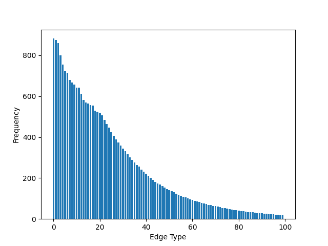
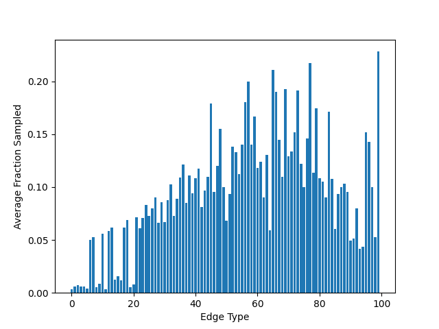
Figure 2: Distribution of edge types in the data (left) and average fraction of edge types sampled in the evaluation (right) for Twosides100.

5.3 Model Configurations and Training

We implemented our proposed approaches on top of R-GAE. Specifically, we introduce learnable edge-type probabilities into the message-passing stage in the R-GCN encoder (RW-GCN) and similar for the probabilistic sampling based on REINFORCE (RS-GCN) (see Section 4.2). We implemented our models in PyTorch and PyTorch Geometric Fey and Lenssen (2019). We use a standard 2-layer R-GCN with hidden dimension of size 128.

We use similar settings for all models and datasets. For Drugbank we use a random 60/20/20 split as suggested in Ryu et al. (2018), and similar for Twosides100. For Drugbank, we use the initial node features from Ryu et al. (2018), where the structural similarity profile of each drug is reduced in its dimension using PCA and then taken as node embedding. For Twosides100, we use one-hot encodings.

We process the target edges in batches using a batch size $b$ of 2000 for Drugbank and of 100 for Twosides100. For each edge in the batch, we sample a fixed size $k$-hop neighborhood around that edge using the sampling procedure described in Section 4.2 with $k=2,s_{1}=7,s_{2}=3$. Additionally, during training, we sample random negative edges for each batch. The amount that we sample is equal to the batch size $b$. We use Adam optimizer with a learning rate of either $0.01$ or $0.001$, train with a patience of 100 epochs, and use binary cross entropy loss.

	Drugbank		Twosides100
Model	PR-AUC	ROC-AUC	PR-AUC	ROC-AUC
DistMult	61.3	96.5	18.5	50.8
DeepDDI	75.0	98.7	28.6	60.7
MPNN	79.1	99.0	36.5	71.0
CompGCN	84.3	98.7	34.0	67.6
R-GAE	80.6	98.9	35.3	67.1
IFR-GAE	81.5	98.9	37.3	71.3
RW-GCN	82.8	99.2	35.7	68.0
RS-GCN	85.6	99.3	39.8	73.3

Table 2: DDI prediction results.

5.4 Results and Discussion

We report our results in Table 2. As commonZitnik et al. (2018), we consider PR-AUC and ROC-AUC as metrics. PR-AUC captures the area under the plot of the precision rate against recall rate at various thresholds. ROC-AUC quantifies the area under the plot of the true positive rate against the false positive rate at various thresholds.

We observe that GNN-based baselines outperform both MLP (DeepDDI) and the tensor factorization based models. This means that the information about the local neighborhood the GNNs encode is indeed useful. The generally lower numbers of Twosides100 can be explained by the fact that it is less dense that Drugbank and it also has a much larger percentage of drug pairs with more than one relation type. In particular, note that the state-of-the-art KG model CompGCN does not always outperform the rather basic R-GAE. That may be due to fact that the properties of DDI graphs are very different from the ones of typical knowledge graphs.

A1 Our incorporation of edge-type probabilities improves prediction accuracy and efficiency.

From Table 2, we observe that RW-GCN and RS-GCN perform overall better than all baselines on both datasets. This shows that giving different importance to different edge types based on the local neighborhood during message passing or neighbor sampling is useful in learning node representations in R-GCN. RS-GCN has an added advantage over RW-GCN since it learns to ignore the less informative neighborhood during the sampling stage only and does not need to take less important edges into account during message passing.

RS-GCN specifically provides an advantage in scalability as shown in Figure 3. Specifically, compared to standard R-GAE (a version without sampling), we obtain an improvement during both training (2.47x) and inference at test time (1.92x); recall that RS-GCN did sampling in both training and inference. PR-AUC is not compromised but even better.

Figure 3: Runtime comparison of RS-GCN to R-GAE with and without random sampling, on Twosides100 validation set. Our RS-GCN converges faster and reaches highest performance.

A2 Learned probabilities offer improvement beyond fixed probabilities based on inverse frequencies.

In order to show that it is indeed beneficial to learn edge-type probabilities, we compare RS-GCN to IFR-GAE. As it is shown in Table 2, on both datasets, IFR-GAE outperforms the other baselines. This is likely due to the fact that both datasets are indeed imbalanced regarding edge types and shows that relation-dependent sampling is an effective means to deal with imbalanced data in general. The distribution of edge types in Twosides100 is depicted in Figure 2 (left). For Drugbank, see Appendix A.

Nevertheless, IFR-GAE does not achieve the performance of our models. One of the reasons behind this is that, even though IFR-GAE takes class imbalance into account during sampling, the sampling probabilities are fixed globally and thus irrespective of the local neighborhoods. On the other hand, the sampling probabilities assigned to different edge types in RS-GCN are calculated adaptively based on the distribution of edge types in the local neighborhood of the target edge. We visualize the assigned probabilities in the $1$-hop neighborhood of a specific edge, whose edge type is to be predicted, in Appendix B. For demonstration purposes, we chose a neighborhood where all edge types occur exactly once. Especially for Twosides100, we can see that, for that particular neighborhood, our model learns probabilities that are different from the ones of IFR-GAE, since they do not reflect the inverse frequency of Twosides100. Apart from capturing and resolving the imbalance of edge types in the data by assigning more weights to rare edge types, our model also learns to assign high weights to some more commonly occurring edge types based on their importance for the current task. Hence, specific, learned probabilities generally reflect importance of edge types better. For Drugbank, the probabilities are similar to the ones learned by IFR-GAE, which means that most edge types are probably of similar importance for this specific example task. However, since the performance of RS-GCN on Drugbank is better than the one of IFR-GAE, the learned probabilities must capture some edge-type-specific information beyond frequency.

Note that IFR-GAE shows better performance than RW-GCN on Twosides100. Together with the fact that RS-GCN outperforms RW-GCN, this confirms that dealing with edge-type probabilities during sampling is generally better than directly adding edge-type importance weights in the model.

Figure 2 (right) further underlines that our relation-specific sampling does not only solve imbalance in the data, but that it makes RS-GCN to better adapt to the link prediction tasks at hand. It shows the actual fractions of edge types sampled during inference averaged over all neighborhoods; hence, it depicts the learned probabilities on a global level. This averaging over the sampled neighborhoods of different target edges in the validation set confirms that, on average, sampling for each type can be different from “simple” inverse frequencies depending on the dataset. Again, the corresponding figure for Drugbank is depicted in Appendix A.

A3 Observations.

Overall, we observe that, for Drugbank, class imbalance has most influence on the learned probabilities. The most commonly occurring DDI (“increase in risk or severity of side effects”) is assigned the lowest probability, and the least occurring DDI (“increase in risk or severity of hyperkalemia”) is assigned the highest probability. On the other hand, consider an example for Twosides100, which has less imbalance. Here, the side effect “traumatic haemorrhage” that has almost the same frequency in our dataset as “stress incontinence” is assigned much higher probability ($0.06$) than latter ($5.6e^{-05}$). We found several examples of this kind.

6 Conclusions

Drug-drug-interaction graphs are large, dense and heterogeneous. In this paper, we propose a new relation-dependent sampling model to solve the scalability issue of graph neural networks on multi-relational graphs (such as DDI graphs). Our experiments on real-world DDI graphs show that RS-GCN outperforms state-of-the-art models in terms of both prediction performance and efficiency.

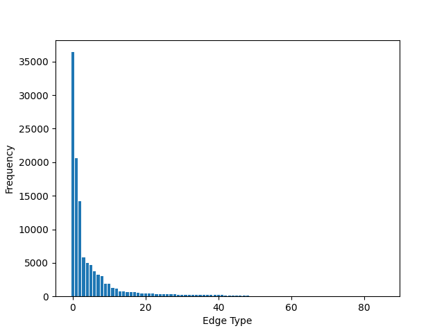
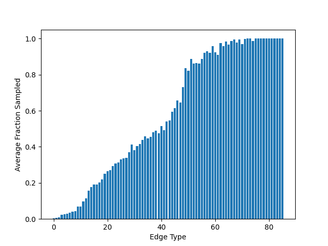
Figure 4: Distribution of edge types in the data (left) and average fraction of edge types sampled in the evaluation (right) for Drugbank.

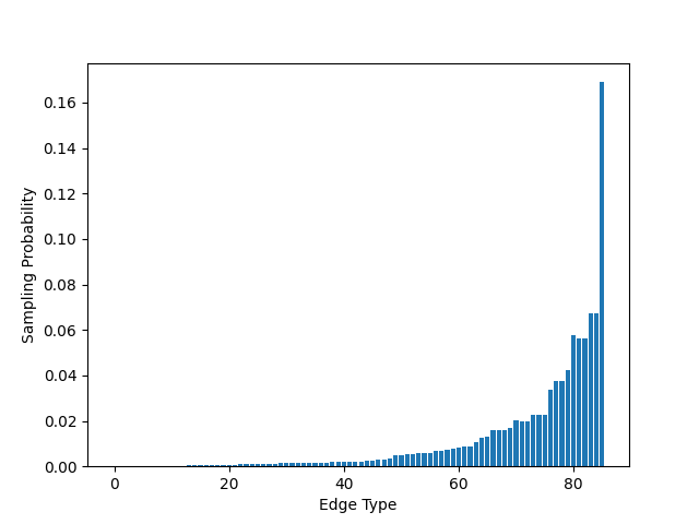
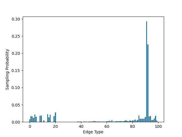
Figure 5: Learned probabilities for an example neighborhood for Drugbank (left) and Twosides100 (right).

Appendix A Edge-Type Frequency and Learned Probabilities for Drugbank

Figure 4 depicts the distribution of edge types in Drugbank and our learned probabilities. The latter are very similar to the inverse frequencies, which means that sampling such that class imbalance is overcome seems to yield highest performance. Hence the edge types must be of similar importance.

Appendix B Additional Results

Figure 5 depicts the probabilities learned for the edge types in an example neighborhood we sampled. While the ones for Drugbank closely reflect the inverse frequencies (compare to Figure 4), the ones for Twosides100 model different patterns of importance.

References

- Bordes et al. [2013] Antoine Bordes, Nicolas Usunier, Alberto Garcia-Duran, Jason Weston, and Oksana Yakhnenko. Translating embeddings for modeling multi-relational data. In Proc. of NeurIPS, pages 2787–2795. 2013.
- Chen et al. [2018a] Jianfei Chen, Jun Zhu, and Le Song. Stochastic training of graph convolutional networks with variance reduction. In Proc. of ICML, pages 942–950, 2018.
- Chen et al. [2018b] Jie Chen, Tengfei Ma, and Cao Xiao. FastGCN: Fast learning with graph convolutional networks via importance sampling. In Proc. of ICLR, 2018.
- DS et al. [2017] Wishart DS, Feunang YD, Guo AC, Lo EJ, Marcu A, Grant JR, Sajed T, Li C Johnson D, Sayeeda Z, Assempour N, Iynkkaran I, Liu Y, Maciejewski A, Gale N, Wilson A, Chin L, Cummings R, Le D, Pon A, Knox C, and Wilson M. Drugbank 5.0: a major update to the drugbank database for 2018. 2017.
- Fey and Lenssen [2019] Matthias Fey and Jan Eric Lenssen. Fast graph representation learning with pytorch geometric. arXiv preprint arXiv:1903.02428, 2019.
- Franceschi et al. [2019] Luca Franceschi, Mathias Niepert, Massimiliano Pontil, and Xiao He. Learning discrete structures for graph neural networks. In Proc. of ICML, 2019.
- Gilmer et al. [2017] Justin Gilmer, Samuel S Schoenholz, Patrick F Riley, Oriol Vinyals, and George E Dahl. Neural message passing for quantum chemistry. In Proc. of ICML, pages 1263–1272, 2017.
- Hamilton et al. [2017] William Hamilton, Rex Ying, and Jure Leskovec. Inductive representation learning on large graphs. In Proc. of NeurIPS, 2017.
- Huang et al. [2018] Wenbing Huang, Tong Zhang, Yu Rong, and Junzhou Huang. Adaptive sampling towards fast graph representation learning. In Proc. of NeurIPS, page 4563–4572, 2018.
- Huang et al. [2019] Kexin Huang, Cao Xiao, Trong Nghia Hoang, Lucas M. Glass, and Jimeng Sun. CASTER: predicting drug interactions with chemical substructure representation. CoRR, abs/1911.06446, 2019.
- Kipf and Welling [2017] Thomas Kipf and Max Welling. Semi-supervised learning with graph convolutional neural networks. In Proc. of ICLR, 2017.
- Lu and Zhou [2011] Linyuan Lu and Tao Zhou. Link prediction in complex networks: A survey. ArXiv, abs/1010.0725, 2011.
- Ma et al. [2018] Tengfei Ma, Cao Xiao, Jiayu Zhou, and Fei Wang. Drug similarity integration through attentive multi-view graph auto-encoders. In Proc. of IJCAI, page 3477–3483, 2018.
- Ma et al. [2019] Tengfei Ma, Junyuan Shang, Cao Xiao, and Jimeng Sun. GENN: predicting correlated drug-drug interactions with graph energy neural networks. CoRR, abs/1910.02107, 2019.
- Ryu et al. [2018] Jae Yong Ryu, Hyun Uk Kim, and Sang Yup Lee. Deep learning improves prediction of drug–drug and drug–food interactions. Proc. of the National Academy of Sciences, 115(18):E4304–E4311, 2018.
- Schlichtkrull et al. [2018] Michael Schlichtkrull, Thomas N Kipf, Peter Bloem, Rianne Van Den Berg, Ivan Titov, and Max Welling. Modeling relational data with graph convolutional networks. In Proc. of ESWC, pages 593–607. Springer, 2018.
- Shang et al. [2019] Chao Shang, Yun Tang, Jing Huang, Jinbo Bi, Xiaodong He, and Bowen Zhou. End-to-end structure-aware convolutional networks for knowledge base completion. In Proc. of AAAI, pages 3060–3067, 2019.
- Tatonetti et al. [2012] Nicholas P. Tatonetti, Patrick Ye, Roxana Daneshjou, and Russ B. Altman. Data-driven prediction of drug effects and interactions. Science translational medicine, 4 125:125ra31, 2012.
- Vashishth et al. [2020] Shikhar Vashishth, Soumya Sanyal, Vikram Nitin, and Partha Talukdar. Composition-based multi-relational graph convolutional networks. Proc. of ICLR, 2020.
- Vilar et al. [2014] Santiago Vilar, Eugenio Uriarte, Lourdes Santana, Tal Lorberbaum, George Hripcsak, and Nicholas Tatonetti. Similarity-based modeling in large-scale prediction of drug-drug interactions. Nature protocols, 9:2147–2163, 09 2014.
- Williams [1992] Ronald J. Williams. Simple statistical gradient-following algorithms for connectionist reinforcement learning. Mach. Learn., 8(3–4):229–256, May 1992.
- Xu et al. [2019] Nuo Xu, Pinghui Wang, Long Chen, Jing Tao, and Junzhou Zhao. MR-GNN: multi-resolution and dual graph neural network for predicting structured entity interactions. Proc. of IJCAI, pages 3968–3974, 2019.
- Xu et al. [2020] Xiaoran Xu, Wei Feng, Yunsheng Jiang, Xiaohui Xie, Zhiqing Sun, and Zhi-Hong Deng. Dynamically pruned message passing networks for large-scale knowledge graph reasoning. Proc. of ICLR, 2020.
- Yang et al. [2015] Bishan Yang, Wen-tau Yih, Xiaodong He, Jianfeng Gao, and Li Deng. Embedding entities and relations for learning and inference in knowledge bases. Proc. of ICLR, 2015.
- Ying et al. [2018] Rex Ying, Ruining He, Kaifeng Chen, Pong Eksombatchai, William L Hamilton, and Jure Leskovec. Graph convolutional neural networks for web-scale recommender systems. In Proc. of KDD, pages 974–983, 2018.
- Zeng et al. [2020] Hanqing Zeng, Hongkuan Zhou, Ajitesh Srivastava, Rajgopal Kannan, and Viktor Prasanna. Graphsaint: Graph sampling based inductive learning method. Proc. of ICLR, 2020.
- Zitnik et al. [2018] Marinka Zitnik, Monica Agrawal, and Jure Leskovec. Modeling polypharmacy side effects with graph convolutional networks. Bioinformatics, 34(13):i457–i466, 2018.