Slow growth of magnetic domains helps fast evolution routes for out-of-equilibrium dynamics

Abstract

Cooling and heating faster a system is a crucial problem in science, technology and industry. Indeed, choosing the best thermal protocol to reach a desired temperature or energy is not a trivial task. Noticeably, we find that the phase transitions may speed up thermalization in systems where there are no conserved quantities. In particular, we show that the slow growth of magnetic domains shortens the overall time that the system takes to reach a final desired state. To prove that statement, we use intensive numerical simulations of a prototypical many-body system, namely, the two-dimensional Ising model.

I Introduction

Nonequilibrium relaxation processes have been extensively studied during the last decades. One important scope in this research is shortening the duration of the heating (or cooling) transient process that precedes thermalization. Indeed, annealing techniques are a popular tool to accelerate the evolution towards the equilibrium—or stationary—state through a slow temperature decrease (not only in physics: the famous simulated annealing algorithm mimics in a computer the annealing strategy followed in the laboratory [1]). Thus, it is not surprising that recent extensions of the counterintuitive Mpemba Effect [2], allowing to cool down faster the hotter of two systems (or heat up faster the cooler system), have stirred considerable attention. Indeed, we now understand which are the general conditions allowing for faster coolings, or faster heatings, in Markovian systems [3, 4], granular matter [5, 6], spin glasses [7], water [8], the quantum Ising spin model [9] and very recently the generalization to Markovian open quantum systems [10]. On these grounds, Amit and Raz have designed a novel strategy, useful in systems with time-scale separation, in which precooling the system results in a faster heating [11].

Yet, time scale separation is not possible at a second-order phase transition, where critical slowing-down [12, 13] evinces a continuum of time scales [see, e.g., Eq. (3) below]. Under these circumstances, unraveling the mechanism that drives the dynamics is the key to potentially control the evolution. The growth of the ordered domains when the system enters the symmetry-broken phase [14, 15, 16] emerges as a natural candidate for this mechanism. Energy is stored in ordered domains whose size and growth arrest or accelerates the dynamics. In particular, the relevance of the domain growth for the dynamic slowdown in spin glasses is now clear [17, 18, 19, 20, 21, 22, 23, 24].

Here we show that the overall relaxation time can be shortened in the absence of time-scale separation by manipulating the system’s internal structure of ordered domains. We focus on the study of the ferromagnetic two-dimensional (2D) Ising spin model. In particular, we study through numerical simulations an unexplored out-of-equilibrium heating protocol, in which the bath temperature starts below the critical temperature and is later heated above the critical point. Surprisingly, we find that this manipulation of the bath temperature induces a speed-up in the energy evolution of the system, which is due to a slow domain-growth process. The mechanism is illustrated by comparing different initial preparation of the system.

This paper is organized as follows: In Sec. II we recall some essential facts about the 2D Ising model and the quantities of interest. The one- and two-step thermal protocols are described in Sec. III, where we also show the number of simulations performed for each protocol. In Sec. IV, we discuss the isothermal evolution of a system in both the ferromagnetic and paramagnetic phases. Section V is devoted to show how the leading time corrections can be canceled out in the two-step protocol. In Sec. VI, we discuss the speed-up of the equilibration procedure for the two-step protocol. The conclusions are contained in Sec. VII. The most technical parts of our work are explained in two Appendixes: In Appendix A, we show how we have implemented the Monte Carlo (MC) dynamics, and in Appendix B, we explain how to perform the spatial integrals of the two-point correlation function.

II Model and quantities of interest

We consider the ferromagnetic Ising model in two dimensions, one of the most thoroughly studied models in statistical mechanics [25]. Specifically, the spins $\sigma_{\bm{x}}=\pm 1$ occupy the nodes $\bm{x}$ of a square lattice of size $L\times L$ with periodic boundary conditions. In our Hamiltonian, the spins interact with their lattice nearest neighbors as

$$\mathcal{H}\;=\;-J\sum_{\langle\bm{x},\bm{y}\rangle}\sigma_{\bm{x}}\sigma_{\bm{y}}\,.$$ (1)

The thermal bath is described through the (dimensionless) inverse-temperature $\kappa=J/(K_{\mathrm{B}}T)$. We have set $J=1$ energy units. A second-order phase transition at $\kappa_{\mathrm{c}}=\log(1+\sqrt{2})/2$ separates the paramagnetic phase at $\kappa<\kappa_{\mathrm{c}}$, from the ferromagnetic phase at $\kappa>\kappa_{\mathrm{c}}$.

We simulate two dynamic rules for the model in Eq. (1): the Metropolis and heat bath (HB) algorithms (see, e.g., [26, 27]). Both belong to the so-called model A dynamic universality class [28], where conserved quantities are lacking. We choose $L=4096$ in our simulations , large enough to represent the thermodynamic limit. Our time step corresponds to a full-lattice sweep. The technical details about how we have implemented both dynamics are contained in Appendix A.

Special attention will be payed to the time evolution of the coherence length $\xi(t)$, namely, the typical linear size of the ferromagnetic domains at time $t$. Note that the correlation length $\xi_{\text{corr}}$ indicates the spatial range of correlations within a domain. Only in the paramagnetic phase $\xi=\xi_{\text{corr}}$. The classification of length scales in the ferromagnetic phase would be even subtler in the presence of Goldstone bosons [30].

Our second important quantity is the energy density $E(t)$, a thermometric quantity [7] for which the equilibrium value $E_{\text{eq}}\equiv E(t\to\infty)$ is given by the well-known Onsager result. Both $E(t)$ and $\xi(t)$ are obtained from the correlation function

$$C(\bm{r};t)\;=\;\frac{1}{L^{2}}\,\sum_{\bm{x}}\left\langle\,\sigma_{\bm{x}}(t)\sigma_{\bm{x}+\bm{r}}(t)\,\right\rangle\,,$$ (2)

where $\langle\ldots\rangle$ indicates the average over $N_{\mathrm{R}}$ independent trajectories or replicas obtained with the same thermal protocol (see next section for the number of replicas used in practice).

Indeed, $E(t)=-2C(\bm{r}_{\circ};t)$, where $\bm{r}_{\circ}=(0,1)$ [or $(1,0)$, because these are the two vectors spanning the square lattice], and $\xi(t)$ is computed from space integrals of $C(\bm{r};t)$ (see also Appendix B).

III Thermal protocols

We consider two distinct thermal protocols, and each of them is simulated twice (with the Metropolis and HB dynamics). In our one-step protocol, a fully disordered spin configuration (corresponding to infinite temperature) is put in contact with a thermal bath at inverse-temperature $\kappa$, at the initial time $t=0$. The coherence length $\xi(t)$ grows with time (see Fig. 1) until (in the paramagnetic phase) its $t\to\infty$ limit is approached.

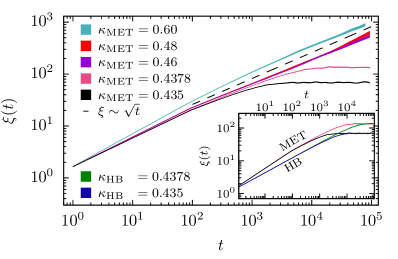
Figure 1: Coherence length $\xi$ as a function of time $t$, as computed with the Metropolis algorithm for our one-step protocol and several values of $\kappa$ (the width of the curves is twice the statistical error; $\kappa$ increases from bottom to top). Only in the paramagnetic phase, $\kappa<\kappa_{\mathrm{c}}\approx 0.44068679$, the coherence length reaches its equilibrium value at long times. In the ferromagnetic phase $\xi(t)\sim\sqrt{t}$ at long times (dashed line). Inset: Comparison of the HB and Metropolis dynamics in the paramagnetic phase. Although $\xi(t)$ grows significantly faster for Metropolis, the equilibrium limit at long times is the same for both dynamics.

In the two-step protocol, a fully disordered spin configuration is initially placed at an inverse temperature in the ferromagnetic phase, $\kappa_{\text{start}}>\kappa_{\text{c}}$, where it evolves until $\xi(t)$ reaches a target value $\xi_{\text{start}}$. At that point, which corresponds with our initial time $t=0$, the bath temperature is instantaneously raised to enter the paramagnetic phase, $\kappa_{\text{end}}<\kappa_{\text{c}}$, and kept fixed afterwards. Note that $\xi_{\text{start}}$ may be larger than $\xi_{\text{end}}\equiv\xi(t\to\infty;\kappa_{\text{end}})$, and that a one-step protocol with $\kappa<\kappa_{\text{c}}$ is a particular case of the two-step protocol with $\xi_{\text{start}}=0$ and $\kappa_{\text{end}}=\kappa$.

We take $\kappa_{\text{end}}=0.435$ and $0.4378$, where $\xi_{\text{end}}$ is very large (see Fig. 1). Indeed, the product $(\kappa_{\mathrm{c}}-\kappa_{\text{end}})\,\xi_{\text{end}}(\kappa_{\text{end}})$ remains constant as $\kappa_{\text{end}}\to\kappa_{\mathrm{c}}$ [25]. This behavior is explained by the fact that the correlation length coincides with the coherence length $\xi$ in the paramagnetic phase, and the value $\nu=1$ of the thermal critical exponent (remember that $\xi_{\text{end}}$ is the coherence length at $\kappa_{\text{end}}$ for long times, when the equilibrium is reached). Of course, this scale invariance is found only close enough to the critical point (in the so-called scaling region). Figure 2 shows that we are indeed working in the scaling region.

For each one of our thermal protocols, and our two dynamics (Metropolis and HB), we have simulated $N_{\mathrm{R}}=256$ replicas with a few exceptions:

1. The one-step protocol with $\kappa=0.435$ (resp. $\kappa=0.4378$), where we have made $1536$ (resp. $4096$) replicas.

2. The two-step protocol with $\kappa_{\text{start}}=0.46$, $\kappa_{\text{end}}=0.4378$ and $\xi_{\text{start}}=120$, where we simulate 1024 replicas.

We have chosen to simulate a larger number of replicas in the paramagnetic phase in order to reduce the statistical error in the correlation function $C(\bm{r};t)$. This error reduction is fundamental for computing the spacial integrals of $C(\bm{r};t)$, from which we compute the coherence length (see Appendix B).

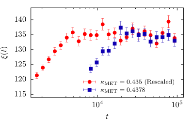
Figure 2: Time evolution of the coherence length in the paramagnetic phase for the one-step protocol for the Metropolis dynamics. The data for $\kappa=0.435$ are multiplied by the scale factor $(\kappa_{\text{c}}-0.435)/(\kappa_{\text{c}}-0.4378)$. Indeed, after the rescaling, the $\kappa=0.435$ data agree at long times with the $\kappa=0.4378$ data, showing that we are in the scaling region (indeed, the thermal critical exponent is $\nu=1$). For later reference, let us quote the value $\xi_{\text{end}}=135(2)$ for the long-time limit at $\kappa=0.4378$.

IV The isothermal evolution

As shown in Fig. 1, the dynamic behavior in the two phases is very different. In the paramagnetic phase, $\kappa<\kappa_{\text{c}}$, both $\xi(t)$ and $E(t)$ approach exponentially their equilibrium value [12, 32]:

$$O(t;\kappa)\;=\;O_{\infty}(\kappa)\,\left[\,1\ -\ \int_{1}^{\tau_{\kappa}}\rho_{O}(\tau,\kappa)\,\text{e}^{-t/\tau}\,\mathrm{d}\tau\right]\,,$$ (3)

where $O(t;\kappa)$ stands for $E(t;\kappa)$ or $\xi(t;\kappa)$, and $\rho_{O}(\tau,\kappa)$ is a continuous distribution of autocorrelation times $\tau$. The largest timescale $\tau_{\kappa}$ (which diverges at $\kappa_{\text{c}}$) ensures that finite-time corrections decay as $\text{e}^{-t/\tau_{\kappa}}$, or faster. Although using Metropolis or HB does make a difference, see the inset of Fig. 1, the equilibrium value at large $t$ is independent of the dynamics.

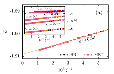
(a)

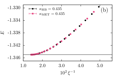
(b)

Figure 3: Energy density $E(t)$ from our one-step protocol as a function of $1/\xi(t)$. (a) Data for $\kappa=0.6$ and both Metropolis and HB dynamics. Both data sets fall on a single curve. The continuous line is a fit to the Ansatz $E(t)=E_{\text{eq}}+b/\xi(t)$. The only free parameter is the slope $b$, and we include only data with $\xi(t)>200$. Inset: Data for several values of $\kappa$, whose value increases from top to bottom. Notice that for a given value of $\kappa$, the Metropolis and HB data sets fall on the same curve. The continuous lines for values of $\kappa$ in the ferromagnetic phase are fits to the Ansatz $E(t;\kappa)=E_{\text{eq}}(\kappa)+b_{\kappa}/\xi(t;\kappa)$ for $\kappa$. Again, the only free parameters are the slopes $b_{\kappa}$, and in each fit, we include only data with $\xi(t)>20$. (b) Data for $\kappa=0.435$ (paramagnetic phase). The solid horizontal line is the exact Onsager solution. The error bars are smaller than the symbols. Notice the null slope at equilibrium, which implies that the growth of the magnetic domains does not affect the energy.

Instead, in the ferromagnetic phase, the largest timescale exists only as a finite-size effect. Indeed, when $\kappa>\kappa_{\text{c}}$ and barring short-time corrections, domains grow as $\xi\sim\sqrt{t}$ [14] until $\xi\sim L$ (see Fig. 1).

Now, it is well known that in the ferromagnetic phase, and excluding fast initial relaxations, $E(t)$ and $\xi(t)$ are tightly connected [12]: $(E(t)-E_{\text{eq}})\propto 1/\xi(t)$, because the excess energy is located at the boundaries of the magnetic domains (and moreover, the lower critical dimension is $1$ for Ising systems). This is the behavior found for $\kappa>\kappa_{\text{c}}$: see Fig. 3(a), and the lower three curves in the inset of that figure. Perhaps more surprisingly, we find that this strong connection extends to the paramagnetic phase where, close to the equilibrium, the magnetic domains grow without changing the system energy [see the top two curves displayed in the inset of Fig. 3(a)]. Indeed [see Fig. 3(b)], if one represents $E(t)$ as a function of $1/\xi(t)$ for $\kappa<\kappa_{\text{c}}$, the data from Metropolis and HB dynamics fall on a single curve (yet, the two time behaviors are remarkably different; see the inset of Fig. 1). Furthermore, notice the null slope of such a curve at equilibrium endpoint [see Fig. 3(b)], which implies that the growth of the magnetic domains does not affect the energy.

The connection between $E(t)$ and $\xi(t)$ suggests an intriguing possibility. Given that $\xi(t)$ grows faster in the ferromagnetic phase (see Fig. 1), it is conceivable that $E(t)$ could equilibrate faster in the paramagnetic phase through an excursion to the ferromagnetic phase.

V Canceling leading time corrections

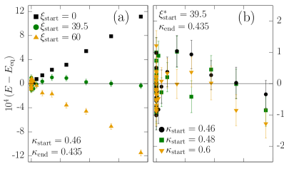
(a)

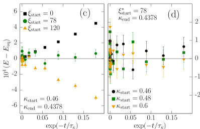
(b)

Figure 4: Excess energy $E(t)-E_{\text{eq}}$ vs $\mathrm{e}^{-t/\tau_{\kappa}}$, as obtained with Metropolis dynamics for our two-step protocol. (a) Data for $\kappa_{\text{start}}=0.46$ and $\kappa_{\text{end}}=0.435$, as computed for several values of $\xi_{\text{start}}$. (b) Data for $\xi_{\text{start}}^{*}=39.5$ and $\kappa_{\text{end}}=0.435$, as computed for several values of $\kappa_{\text{start}}$. (c) As in panel (a), for $\kappa_{\text{start}}=0.46$ and $\kappa_{\text{end}}=0.4378$. (d) As in panel (b), for $\xi_{\text{start}}^{*}=78$ and $\kappa_{\text{end}}=0.4378$.

As suggested by Eq. (3), in the paramagnetic phase, the two-step protocol behaves at long times as (see Fig. 4 for the Metropolis dynamics and Fig. 5 for the HB one):

$$E(t)-E_{\text{eq}}\;=\;{\mathcal{A}}\,(\xi_{\text{start}})\,\mathrm{e}^{-t/\tau_{\kappa}}\,,$$ (4)

where ${\mathcal{A}}(\xi_{\text{start}})$ is an amplitude (the one-step protocol is recovered for $\xi_{\text{start}}=0$). Interestingly enough, ${\mathcal{A}}(\xi_{\text{start}})$ changes sign as the initial coherence length grows. This phenomenon is clearly seen in Figs. 4(a)-4(c) and 5(a)-5(c). It follows that there exists a $\xi_{\text{start}}^{*}$ such that ${\mathcal{A}}(\xi_{\text{start}}^{*})=0$, which entails an exponential speed-up. It turns out that $\xi_{\text{start}}^{*}$ is independent of $\kappa_{\text{start}}$ [see Figs. 4(b)-4(d) and 5(b)-5(d)]. However, computing $\xi_{\text{start}}^{*}$ is difficult because of the statistical uncertainty in $\mathcal{A}(\xi_{\text{start}})$.

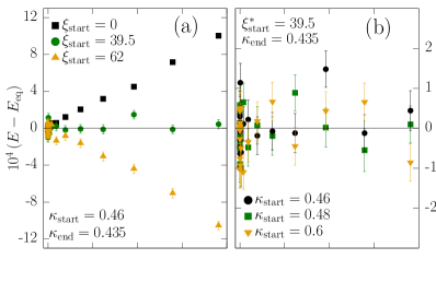
(a)

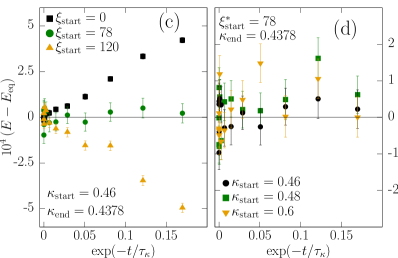
(b)

Figure 5: Excess energy $E(t)-E_{\text{eq}}$ vs $\mathrm{e}^{-t/\tau_{\kappa}}$, as obtained with the HB dynamics for our two-step protocol. (a) Data for $\kappa_{\text{start}}=0.46$ and $\kappa_{\text{end}}=0.435$, as computed for several values of $\xi_{\text{start}}$. (b) Data for $\xi_{\text{start}}^{*}=39.5$ and $\kappa_{\text{end}}=0.435$, as computed for several values of $\kappa_{\text{start}}$. (c) As in panel (a), for $\kappa_{\text{start}}=0.46$ and $\kappa_{\text{end}}=0.4378$. (d) As in panel (b), for $\xi_{\text{start}}^{*}=78$ and $\kappa_{\text{end}}=0.4378$.

In order to estimate $\xi_{\text{start}}^{*}$ we have taken several values of $\xi_{\text{start}}$ around our initial guess for $\xi_{\text{start}}^{*}$, obtained from Fig. 4 (Metropolis) and Fig. 5 (HB). The value of $\tau_{\kappa}$ in Eq. (4) is estimated by fitting to the Ansatz (4) our most accurate data, namely, that with $\xi_{\text{start}}=0$. We then estimate $\mathcal{A}(\xi_{\text{start}})$ using the same Ansatz (4) with $\tau_{\kappa}$ fixed to the previously obtained value. We have chosen the fitting window as $0\leq\text{e}^{-t/\tau_{\kappa}}\leq 0.2$.

Our strategy consists in finding an interval $(\xi_{\text{start}}^{+},\xi_{\text{start}}^{-})$ where $\xi_{\text{start}}^{*}$ is contained (see Tables 1 and 2). We require $\mathcal{A}$ to be positive (resp. negative) with high probability (i.e., larger in absolute value than twice its statistical error) at $\xi_{\text{start}}^{+}$ (resp. $\xi_{\text{start}}^{-}$). Finally, we estimate the value of $\xi_{\text{start}}^{*}$ as the average of $\xi_{\text{start}}^{+}$ and $\xi_{\text{start}}^{-}$, and its error as the semi-difference of $\xi_{\text{start}}^{+}$ and $\xi_{\text{start}}^{-}$ (see Table 3).

$\xi_{\text{start}}$	$\mathcal{A}\ \times 10^{4}$	$|\mathcal{A}|/\Delta\mathcal{A}$
$37\phantom{.5}$	$10.6(18)$	$5.9$
$39.5$	$\phantom{-}0.8(20)$	$0.4$
$42\phantom{.5}$	$-4.6(18)$	$2.6$

(a) Metropolis

$\xi_{\text{start}}$	$\mathcal{A}\ \times 10^{4}$	$|\mathcal{A}|/\Delta\mathcal{A}$
$36\phantom{.5}$	$\phantom{-}13(2)\phantom{.91}$	$\phantom{1}6.5$
$39.5$	$\phantom{-2}3(2)\phantom{.91}$	$\phantom{1}1.5$
$50\phantom{.5}$	$-26.3(19)$	$13.8$

(b) Heat bath

Table 1: Values of $\mathcal{A}(\xi_{\text{start}})$ obtained with $\kappa_{\text{start}}=0.46$ and $\kappa_{\text{end}}=0.435$ for the Metropolis (a) and HB (b) dynamics. $\Delta\mathcal{A}$ is the statistical error obtained from the fit to Eq. (4). The value of $\tau_{\kappa}$ used to fit the data is 433(14) for Metropolis, and 1470(50) for HB.

$\xi_{\text{start}}$	$\mathcal{A}\times 10^{4}$	$|\mathcal{A}|/\Delta\mathcal{A}$
$70$	$\phantom{-}5(2)\phantom{.91}$	$2.5$
$79$	$-2(2)\phantom{.91}$	$1\phantom{.5}$
$87$	$-5.0(19)$	$2.6$

(a) Metropolis

$\xi_{\text{start}}$	$\mathcal{A}\times 10^{4}$	$|\mathcal{A}|/\Delta\mathcal{A}$
$70\phantom{.5}$	$\phantom{-}9(2)$	$4.5$
$81.5$	$-1(3)$	$0.3$
$92\phantom{.5}$	$-8(3)$	$2.7$

(b) Heat bath

Table 2: Values of $\mathcal{A}(\xi_{\text{start}})$ obtained with $\kappa_{\text{start}}=0.46$ and $\kappa_{\text{end}}=0.4378$ for the Metropolis (a) and HB (b) dynamics. $\Delta\mathcal{A}$ is the statistical error obtained from the fit to Eq. (4). The value of $\tau_{\kappa}$ used to fit the data is 2000(100) for Metropolis, and 6500(300) for HB.

$\kappa_{\text{end}}=0.435$		$\kappa_{\text{end}}=0.4378$
MET	HB	MET	HB
40(3)	43(7)	79(9)	81(11)

Table 3: $\xi_{\text{start}}^{*}$ estimate for the Metropolis (MET) and HB dynamics for each value of $\kappa_{\text{end}}$. The center value and its error are obtained from the semisum and semidifference of the extreme values from the Tables 1 and 2.

The final results for $\xi_{\text{start}}^{*}$ shows a compatibility between both dynamics (see Table 3). The values of $\xi_{\text{start}}^{*}$ should be compared with the coherence length at equilibrium $\xi_{\text{end}}(\kappa)$, namely, $\xi_{\text{end}}(0.435)=69(1)$ and $\xi_{\text{end}}(0.4378)=135(2)$, both for the Metropolis dynamics.

Furthermore, when $\kappa_{\text{end}}$ is varied, both $\xi_{\text{start}}^{*}$ and the equilibrium coherence length $\xi_{\text{end}}$ scale as $1/(\kappa_{\mathrm{c}}-\kappa_{\text{end}})$.

These two traits, namely, independence of $\kappa_{\text{start}}$ and the correct scaling dimension for $\xi_{\text{start}}^{*}$, are hallmarks of universality. Indeed, we speculate that the scale-invariant ratio that we find for the Metropolis dynamics

$$\lim_{\kappa\to\kappa_{\mathrm{c}}^{-}}\frac{\xi_{\text{start}}^{*}}{\xi_{\text{end}}}\;=\;0.59(7)$$ (5)

will be common to all models with scalar order parameter in the model A dynamic universality class [28]. Our results for the HB dynamics are indeed consistent with this speculation.

VI Equilibration speed-up

Let us put to use the existence of an exponential speed-up. From now on, we shall be referring to $t_{\text{total}}$, namely, the time spent by the system at both $\kappa_{\text{start}}$ and $\kappa_{\text{end}}$. In fact, we operationally define the equilibration time $t^{0.1\%}_{\text{eq}}$ as the time such that $E(t_{\text{total}})$ differs from $E_{\text{eq}}$ by less than 0.1% for any $t_{\text{total}}>t^{0.1\%}_{\text{eq}}$; see Fig. 6 . In other words, the equilibration time $t^{0.1\%}_{\text{eq}}$ corresponds to the last time the energy crosses either the line $1.001E_{\text{eq}}$ or the line $0.999E_{\text{eq}}$ (see Fig.7). We need this operational definition because, strictly speaking, thermal equilibrium is unreachable in any finite time.

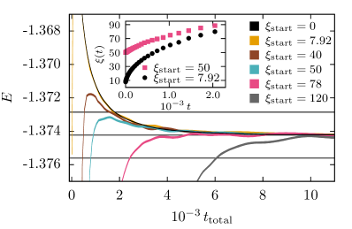
Figure 6: Energy density as a function of the total time $t_{\text{total}}$ elapsed since the beginning of the two-step protocol, as computed with the Metropolis dynamics for $\kappa_{\text{start}}=0.46$, $\kappa_{\text{end}}=0.4378$, and several values of $\xi_{\text{start}}$. These values of $\xi_{\text{start}}$ increase from top to bottom. The width of the curves is twice the statistical errors. We show only the evolution during the second step of the protocol. The three horizontal lines correspond to $E_{\text{eq}}$ multiplied by $1.001,1$ and $0.999$. Inset: Coherence length during the two-step protocol ($\kappa_{\text{start}}=0.46$, $\kappa_{\text{end}}=0.4378$) as a function of the time $t$ elapsed since the temperature changed. We show data for $\xi_{\text{start}}^{\text{Kovacs}}\approx 7.92$ (lower curve), as well as for $\xi_{\text{start}}=50$ (upper curve; this value yields the minimum equilibration time; see Fig. 7).

Now, let us consider the situation for the two-step protocol with $\xi_{\text{start}}<\xi_{\text{start}}^{*}$ and where ${\cal A}(\xi_{\text{start}})>0$ [cf., Eq. (4)]. In this range of small $\xi_{\text{start}}$ we encounter $\xi_{\text{start}}=\xi_{\text{start}}^{\text{Kovacs}}$ where the energy at the time of the temperature change equals $E_{\text{eq}}$ (this is the appropriate situation to study the Kovacs effect [34, 18]). Now, for those protocols with $\xi_{\text{start}}^{\text{Kovacs}}<\xi_{\text{start}}<\xi_{\text{start}}^{*}$ , the energy at the time the temperature changes is smaller than $E_{\text{eq}}$  but, at long times, $E(t_{\text{total}})$ tends to $E_{\text{eq}}$ from above because ${\cal A}(\xi_{\text{start}})>0$. It follows that $E(t_{\text{total}})$ cannot be monotonic. In fact (see Fig. 6), $E(t_{\text{total}})$ for those protocols first grow to a local maximum, then decrease towards $E_{\text{eq}}$.

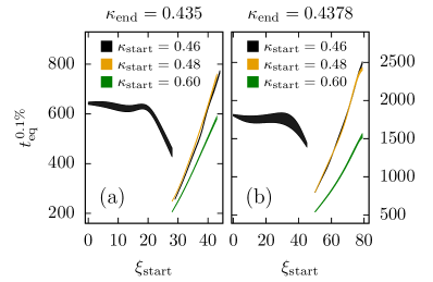
Figure 7: Equilibration time $t^{0.1\%}_{\text{eq}}$ versus $\xi_{\text{start}}$ for the two-step protocol with $\kappa_{\text{end}}=0.435$ (a) and $\kappa_{\text{end}}=0.4378$ (b). We show data for three values of $\kappa_{\text{start}}$ and the Metropolis dynamics. The width of the curves is twice the statistical errors. The discontinuity is due to the nonmonotonic time behavior of $E(t_{\text{total}})$; see Fig. 6. Note that, after the discontinuity, the curves for $\kappa_{\text{start}}=0.46$ and $\kappa_{\text{start}}=0.48$ are very close.

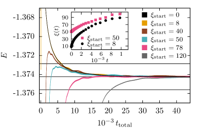
Figure 8: Energy density as a function of the total time $t_{\text{total}}$ elapsed since the beginning of the two-step protocol, as computed with the HB dynamics for $\kappa_{\text{start}}=0.46$, $\kappa_{\text{end}}=0.4378$, and several values of $\xi_{\text{start}}$. Plot definitions are as in Fig. 6. Inset: Coherence length during the two-step protocol ($\kappa_{\text{start}}=0.46$, $\kappa_{\text{end}}=0.4378$) as a function of the time $t$ elapsed since the temperature changed. We show data for $\xi_{\text{start}}^{\text{Kovacs}}\simeq 8$ (lower curve), as well as for $\xi_{\text{start}}=50$ (upper curve; this value yields the minimum equilibration time; see Fig. 9).

The local maximum of $E(t_{\text{total}})$ entails a discontinuity for the equilibration time $t^{0.1\%}_{\text{eq}}$ (cf., Fig. 7) at the value of $\xi_{\text{start}}$ for which the height of the local maximum of $E(t_{\text{total}})$ coincides with the upper limit of the $0.1\%$ band around $E_{\text{eq}}$ . Therefore, the equilibration time $t^{0.1\%}_{\text{eq}}$ for the two-step protocols just after the discontinuity could be shorter than its one-step counterpart by a factor of three.

We can repeat the above computations for the HB dynamics. If we represent the energy density vs the total simulation time $t_{\text{total}}$, we obtain Fig. 8. The plot of the equilibration time $t_{\text{eq}}^{0.1\%}$ as a function of $\xi_{\text{start}}$ is given by Fig. 9. The behavior of these two quantities is analogous to the one found for Metropolis. The main difference is the time scale. Indeed, Metropolis approaches equilibrium faster than HB.

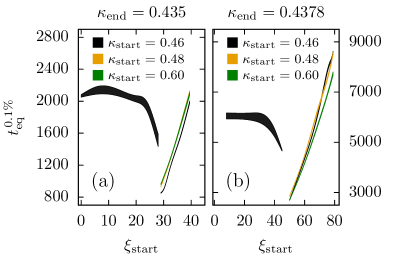
Figure 9: Equilibration time $t_{\text{eq}}^{0.1\%}$ as function of $\xi_{\text{start}}$ for the two-steps protocol with $\kappa_{\text{end}}=0.435$ (a) and $\kappa_{\text{end}}=0.4378$ (b). We show data for three values of $\kappa_{\text{start}}$ and the HB dynamics. Plot definitions are as in Fig. 7. The discontinuity is due to the nonmonotonic time behavior of $E(t_{\text{total}})$, see Fig. 8. Note that, after the discontinuity, the curves for $\kappa_{\text{start}}=0.48$ and $\kappa_{\text{start}}=0.60$ are very close in (a), and the curves for $\kappa_{\text{start}}=0.46$ and $\kappa_{\text{start}}=0.48$ are very close in (b).

VII Conclusions

We have shown that precooling may result in faster equilibration at higher temperatures in a prototypical system without timescale separation (namely, the ferromagnetic 2D Ising model at its critical point). The driving mechanism is the tight connection between the internal energy and the size of the ferromagnetic domains, characteristic of a broken-symmetry phase [12]. Indeed, the size of the domains can be manipulated to our advantage through a nonequilibrium protocol. In particular, we have found an exponential speed-up in the equilibration of the energy. The speed-up arises when the size of the magnetic domains formed during the excursion to the low-temperature phase is a well-defined fraction of the equilibrium correlation-length at the higher temperature. We have found numerical evidence for the universality of this fraction (presumably, the universality is restricted to model A dynamics with scalar order parameter [28]). Namely, we have shown how to design a practical protocol that exploits this universal mechanism.

Appendix A Implementation of multisite multispin algorithm

Nowadays, many CPUs support 256-bit words in their streaming extensions. This allows us to perform basic Boolean operations (AND, XOR, etc.) in parallel for all the 256 bits, in a single clock cycle. We can take advantage from this parallelization by codifying 256 distinct spins in the same 256-bit word. This strategy is called multispin coding [37]. Furthermore, we simulate a single system, so we pack 256 spins from the same lattice. This is known as MUlti-SIte (MUSI) multispin coding (or Synchronous multispin coding [38]). The main problem with MUSI multispin coding is generating 256 independent random numbers for the 256 spins coded in a word. A careless approach to the generation of these 256 random numbers would break the parallelism, thus making MUSI multispin coding useless.

For the sake of clarity, we explain first our geometrical set up, and then describe how we solved the problem of the independent random number for each spin in the 256-bit word.

A.1 Our multispin coding geometry

In our MUSI simulation, we packed 256 spins, from the same lattice, in a single 256-bits word, forming a superspin [39]. Specifically, we employed the packing introduced in Ref. [32]. We present the packing for a $M^{2}$-bit computer word (we shall specialize to $M=16$, and $M^{2}=256$ bits). This packing transforms the original square lattice of size $L\times L$ into a superspin lattice of size $(L/M)\times(L/M)$. The physical coordinates $\bm{x}=(x,y)$ and the superspin coordinates $(i_{x},i_{y})$ are related by:

$$\begin{split}x\;=\;\ &b_{x}\frac{L}{M}+i_{x},\text{ where}\\ &b_{x}\;=\;0,1,\cdots,M-1;\text{ and}\\ &i_{x}\;=\;0,1,\cdots,\frac{L}{M}-1\,.\end{split}$$ (6)

$$\begin{split}y\;=\;\ &b_{y}\frac{L}{16}+i_{y},\text{ where}\\ &b_{y}\;=\;0,1,\cdots,M-1;\text{ and}\\ &i_{y}\;=\;0,1,\cdots,\frac{L}{M}-1\,.\end{split}$$ (7)

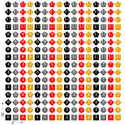
Figure 10: Graphical representation of the packing process of a square lattice of size $16\times 16$ using 16-bit computer word (hence, $M=4$ in this example). The packing results into a $16/4\times 16/4$ superspin lattice. The symbols represent the $i_{x}$ coordinate, and the colors represent the $i_{y}$ coordinate. Therefore, all spins with same symbol and color are codified in the same superspin. The number inside the symbol is the bit index $i_{b}=Mb_{y}+b_{x}$. Consider the spin at site $(x,y)$ and its neighbor along the (say) forward $x$-direction, with $x$ coordinate $(x+1)\mod L$. This neighbor is packed in the forward $x$-direction neighbor superspin, with $(i_{x}+1)\mod(L/M)$ coordinate. If $i_{x}<L/M-1$, the coordinates $i_{y},b_{x}$ and $b_{y}$ remain unchanged [if $i_{x}=L/M-1$, $b_{x}$ changes when going forward along the $x$-direction as $b_{x}\rightarrow(b_{x}+1)\mod M$].

As a consequence, $M^{2}$ physical coordinates $(x,y)$ are assigned to the very same superspin coordinates $(i_{x},i_{y})$. The bit index $i_{b}=Mb_{y}+b_{x}$ is the position inside the superspin (so $0\leq i_{b}<M^{2}$), and unambiguously identifies the physical coordinates (see Fig. 10 for a graphical example of the packing process of a $L=16$ square lattice using $M=4$).

There is a crucial feature of our chosen geometry. Take a superspin $(i_{x},i_{y})$. Each of the $M^{2}$ spins packed in the superspin $(i_{x},i_{y})$ has a nearest neighbor along the (say) forward $x$-direction in the original lattice. All these $M^{2}$ neighboring spins are themselves packed in the same superspin, namely, the nearest neighbor in the forward $x$-direction in the superspin lattice (see Fig. 10).

Another important property of Eqs. (6) and (7) is that the parity of the superspin site $i_{x}+i_{y}$ and the original site parity $x+y$ coincide (provided that $L/M=2n$, with $n\in\mathbb{N}$). Note that the square lattice is bipartite: with our nearest-neighbor interactions, sites of even parity interact only with odd-parity sites (and vice versa). This feature suggests a checkerboard updating scheme, in which all even sites are update in the first step and odd sites are updated afterwards. Indeed, keeping the (say) odd spins fixed, the ordering of the update of the even spins is immaterial. In particular, we may update simultaneously the 256 spin that we pack in a superspin.

We define our time unit as a full-lattice sweep, in which the even sublattice is updated first and the odd superspins are updated afterwards.

A.2 Random numbers

For reasons of clarity, we shall be referring always to a single bit, $s_{\bm{x}}(t)$, in the superspin [$s_{\bm{x}}(t)=1$ if the spin it codes is 1 at time $t$, while the bit is zero if the spin is $-1$]. All the Boolean operations that we shall explain below are performed simultaneously on the 256 bits $s_{\bm{x}}(t)$ contained in the superspin.

The scope of the game is obtaining a change bit $B_{\bm{x}}(t)$, which is one if (and only if) the spin at site $\bm{x}$ is to be flipped at MC time $t$:

$$s_{\bm{x}}(t+1)\;=\,s_{\bm{x}}(t)\text{ XOR }B_{\bm{x}}(t)\,.$$ (8)

The computation of $B_{\bm{x}}(t)$ is naturally decomposed in two steps (the first is a deterministic step, while the second step involves randomness):

1. In the first step, we compute the energy change $\Delta E$ that flipping spin $s_{\bm{x}}(t)$ would cause. Now, $\Delta E$ can take five values, $\Delta E\in\{-8,-4,0,4,8\}$. Hence using standard Boolean operations, one computes five bits $\{c_{\bm{x}}^{-8}(t),\ c_{\bm{x}}^{-4}(t),\ c_{\bm{x}}^{0}(t),\ c_{\bm{x}}^{4}(t),\ c_{\bm{x}}^{8}(t)\}$ in such a way that only the bit with superscript equal to $\Delta E$ is one. The remaining four bits are, of course, zero.

2. The second step depends on the dynamics, either Metropolis or HB, and determines whether or not the spin-flip is allowed. This is represented by other five bits $\{b_{\bm{x}}^{-8}(t),\ b_{\bm{x}}^{-4}(t),\ b_{\bm{x}}^{0}(t),\ b_{\bm{x}}^{4}(t),\ b_{\bm{x}}^{8}(t)\}$, which are set to one with probability $p(\Delta E)$, as we explain below.

We obtain $B_{\bm{x}}(t)$ from these bits as (for brevity, we will omit their dependence on $\bm{x}$ and $t$):

$$\begin{split}B\;=\;&\ [c^{8}\text{ AND }b^{8}]\text{ OR }[c^{4}\text{ AND }b^{4}]\\ &\text{ OR }[c^{0}\text{ AND }b^{0}]\text{ OR }[c^{-4}\text{ AND }b^{-4}]\\ &\text{ OR }[c^{-8}\text{ AND }b^{-8}].\end{split}$$ (9)

A.2.1 The probabilities

The probabilities for setting to one the random bits $b$ depend on the precise algorithm we are using:

1. Metropolis:

   $$p_{\text{MET}}(\Delta E)\;=\;\text{min}\{1,e^{-\Delta E/T}\}\,,$$ (10)

2. Heat-bath:

   $$p_{\text{HB}}(\Delta E)\;=\;\displaystyle\frac{e^{-\Delta E/T}}{1+e^{-\Delta E/T}}\,.$$ (11)

A.2.2 Some remarks on statistical independence

Equation (9) tells us that we are going to use only one of the five bits $b$, although we cannot know in advance which one. Indeed, the AND conditions make irrelevant those bits $b$ whose superscript differ from $\Delta E$. Hence, the five $b$ bits do not need to be mutually independent (instead, the $b$ bits corresponding to different $\bm{x}$ or $t$ must be statistically independent). We can make use of this observation to reduce the number of $b$ bits that we need to compute:

1. In the Metropolis dynamics, we only need two bits because $p_{\text{MET}}(\Delta E)=1$ for $\Delta E\leq 0$. Therefore, we set $b^{-8}=b^{-4}=b^{0}=1$.

2. In the HB dynamics, because $p_{\text{HB}}(\Delta E)=1-p_{\text{HB}}(-\Delta E)$, we set $b^{-8}=\text{ NOT }b^{8}$ and $b^{-4}=\text{ NOT }b^{4}$.

A.2.3 Generating independent random bits with arbitrary probability

As we have seen, we need to generate a stream of independent random bits, which are set to one with a probability $p$ given by Eq. (10) or (11). The textbook solution [38] fails the independence requirement (unless $p$ can be exactly represented with a small number of bits). On the other hand, the rather high critical temperature in our problem makes the Gillespie method [39] inefficient because $p$ is too large. We solve this problem by adapting a strategy [40] that somewhat interpolates between the textbook and the Gillespie methods.

To simplify the explanation, let us consider only one of the five bits $\{b^{-8},\ b^{-4},\ b^{0},\ b^{4},\ b^{8}\}$, for example $b^{4}$. We obtain $b^{4}$ as $b^{4}=d_{1}\text{ OR }d_{2}$, where $d_{1}$ and $d_{2}$ are two independent random bits which are set to one with probabilities $p_{1}$ and $p_{2}$, respectively. It is easy to check that the probability $p(4)$ for having $b^{4}=1$ is $p(4)=p_{1}+p_{2}(1-p_{1})$. Hence, if we choose $p_{1}$ in some convenient way (see below), we need to set $p_{2}$ as

$$p_{2}\;=\;\frac{{p(4)}-p_{1}}{1-p_{1}}\,.$$ (12)

The overall idea is the following: if we can efficiently generate $d_{1}$ with a probability $p_{1}$ very close to (but smaller than) $p(4)$, we will find ourselves with a $p_{2}$ small enough for an efficient use of the Gillespie method.

Specifically, we require that $p_{1}$ be exactly representable with $m$ bits

$$\begin{split}p_{1}&\;=\;\frac{k^{*}+1}{2^{m}},\text{ with }k^{*}\in\mathbb{N},\ 0\;\leq\;k^{*}<2^{m},\ \text{ and }\\ &\frac{k^{*}+1}{2^{m}}\;\leq\;{p(4)}\;<\;\frac{k^{*}+2}{2^{m}}\,.\end{split}$$ (13)

We obtain $d_{1}$ by generating an integer-valued random number $k$, $0\leq k<2^{m}$, with uniform probability. We set $d_{1}=1$ if $k\leq k^{*}$.

Notice that $m$ determines the efficiency of the algorithm. On one hand, enlarging $m$ can be detrimental because we generate $k$ by obtaining $m$ independent random bits which are set to one with $50\%$ probability. On the other hand, a large $m$ allows us to have $p_{1}$ very close to $p(\Delta E)$, and hence a very small $p_{2}$. A tradeoff needs to be found, by minimizing the total number of calls to our random number generator.

An important simplification is that we are allowed to use the same random integer $k$ for all the $\Delta E$, only the threshold $k^{*}(\Delta E)$ varies. In this way, we obtain all the bits $d_{1}$ for every $b^{8}$ and $b^{4}$.

As for the second bit $d_{2}$, we have two different probabilities $p_{2}$, one for $b^{8}$ [$p_{2}(8)$], and other for $b^{4}$ [$p_{2}(4)$]. Let $p_{\text{max}}=\text{max}\{p_{2}(4),p_{2}(8)\}$ and $p_{\text{min}}=\text{min}\{p_{2}(4),p_{2}(8)\}$, so we can implement the Gillespie method for $p_{\text{max}}$, which gives the bits $d_{2}$ for the $\Delta E$ with bigger $p_{2}$ probability. The bit $d_{2}$ corresponding to $p_{\text{min}}$ is set to one if two conditions are met: (1) the bit $d_{2}$ corresponding to $p_{\text{max}}$ is set to one, and (2) an independent random number $r$, extracted with uniform probability in $[0,1)$, turns out to be smaller than $p_{\text{min}}/p_{\text{max}}$.

Finally, we need to discuss our computation of the random integers $k$. In fact, we need to generate 256 independent $k$ numbers, because we codify 256 spins in our superspins. After some reflection, we decided to use the xoshiro256++ generator [41], which ensures the same level of randomness on each of its 64-bits. We employed a 256-bits streaming extension to implement a parallel version of xoshiro256++, composed of four independent xoshiro256++ random sequences. Hence, each call to our generator produces 256 independent random bits which are 1 with $50\%$ probability. Therefore, $m$ calls to xoshiro256++ produces 256 independent $k$ random numbers.

In our simulations, the optimal value of $m$ has turned out to be $m\simeq 10$. In this way, we have found it possible to compute the spin-flip bit for 1024 spins with approximately 42 calls to our random number generators (namely, 40 calls for $d_{1}$ and two calls for the computation of $d_{2}$).

Appendix B Space integrals of $\bm{C(\bm{r};t)}$ correlation

At long distances, the correlation function $C(\bm{r};t)$ decays as $f(-r/\xi(t))/r^{a}$, where $\xi$ is the coherence length, $f(x)$ is a cut-off function, and $a$ is an exponent. Out-of-equilibrium, the function $f(x)$ decays super-exponentially, while, at equilibrium, the decay is only exponential. Unfortunately, the exponent $a$ and the precise form of the function $f(x)$ are known only at equilibrium. Nevertheless, following Ref. [19], we can obtain $\xi(t)$ from an integral estimator.

Hereafter, we shall use $C(r;t)$ as a shorthand for $C(\bm{r};t)$ with $\bm{r}=(r,0)$ or $\bm{r}=(0,r)$. Introducing the integrals

$$I_{k}(t)\;=\;\int_{0}^{\infty}r^{k}C(r;t)\,\mathrm{d}r\,,$$ (14)

we can define $\xi_{k,k+1}(t)\equiv I_{k+1}(t)/I_{k}(t)$, which is proportional to $\xi(t)$. In our case, we have chosen as an estimator of $\xi(t)$ the ratio $\xi_{1,2}(t)$, which has been well studied in the literature (see e.g., Refs. [42, 22, 32], and references therein).

The difficulty in the computation of this integrals arises from the big relative errors $[\Delta C(r;t)/C(r;t)]$ present in the large-$r$ tail of $C(r;t)$ (this problem is well known in the context of the analysis of autocorrelation times in MC simulations [26]). Our solution, which is inspired by Ref. [42, 22, 32], combines two strategies: (1) reduction of the relative error in the correlation function by considering a sufficiently large number of replicas (see Sec. III), and (2) the use of a smart way to estimate $I_{k}(t)$. Our estimation of $I_{k}(t)$ is the sum of two contributions: the numerical integral of our measured $C(r;t)$ up to a noise-dependent cut-off, and a tail contribution estimated by using a smooth extrapolation function, namely, $F(r)=A\text{e}^{-(r/\xi_{F})^{\beta}}/r^{b}$ with $b=1/2$.

Strictly speaking, the functional form of $F(r)$ is only valid in the paramagnetic phase [42]. In the ferromagnetic phase, the exponent of the algebraic term $r^{b}$ is not known. However, because the exponential term decays very fast ($\beta\approx 2$), the precise value of $b$ is not very relevant. On the other hand, when the equilibrium is reached in the paramagnetic phase, where $\beta=1$, the slow decay of $C(r,t)$ makes the tail contribution very relevant (this is why we have needed a large number of replicas in order to have a good estimation of the tail contribution in the paramagnetic phase).

The complete procedure to compute $I_{k}$ is as follows:

1. We obtain a spatial cut-off determined by the size of our statistical errors. The noise-dependent distance $r_{\mathrm{cut}}$ is the shortest distance such that $C(r_{\mathrm{cut}}+1;t)$ is smaller than three times its error. Of course, $r_{\mathrm{cut}}$ is time-dependent.

2. Estimate the region $[r_{\mathrm{min}},r_{\mathrm{max}}]$ employed in the fit to $F(r)$. We start by locating the position $r^{*}$ of the maximum of the quantity $r^{2}C(r;t)$; the value of such maximum is $\rho={r^{*}}^{2}C(r^{*};t)$. Next, we determine $r_{\mathrm{min}}$ and $r_{\mathrm{max}}$, which must verify the inequalities $r^{*}<r_{\mathrm{min}}<r_{\mathrm{max}}<r_{\mathrm{cut}}$. We define $r_{\mathrm{min}}$ (resp. $r_{\mathrm{max}}$) as the first $r$ where $r^{2}C(r;t)<a_{\mathrm{min}}\rho$ (resp. $r^{2}C(r;t)<a_{\mathrm{max}}\rho$). We take $a_{\mathrm{min}}=0.9$ and $a_{\mathrm{max}}=1/3$. We regard a failure to meet the condition $r_{\mathrm{max}}<r_{\mathrm{cut}}$ as a sure-tell sign of the need of increasing the number of replicas.

3. Finally we calculate the integrals. There are two possibilities (in both cases we estimate errors with the jackknife method [43, 44]):

   1. If $r_{\mathrm{max}}-r_{\mathrm{min}}>8$, we fit $C(r;t)$ in the interval $[r_{\mathrm{min}},r_{\mathrm{max}}]$ to $F(r)$ (the fit parameters are the amplitude $A$, the length scale $\xi_{F}$, and the exponent $\beta$). We estimate the integral as the sum of two contributions, namely, the integral of $C(r;t)$ from $r=0$ to $r_{\mathrm{max}}$ and the integral of $F(r)$ from $r_{\mathrm{max}}$ to $r=20\xi_{F}$. In both terms, we use a second-order Gaussian quadrature (when an interpolation of $C(r;t)$ is needed, we employ a cubic spline interpolation).

   2. If the region $[r_{\mathrm{min}},r_{\mathrm{max}}]$ is small (i.e. $r_{\mathrm{max}}-r_{\mathrm{min}}\leq 8$), we integrate only numerically $C(r;t)$ up to $r_{\mathrm{cut}}$.

References

- Kirkpatrick et al. [1983] S. Kirkpatrick, C. D. Gelatt, and M. P. Vecchi, Optimization by simulated annealing, Science 220, 671 (1983).
- Mpemba and Osborne [1969] E. B. Mpemba and D. G. Osborne, Cool?, Phys. Educ. 4, 172 (1969).
- Lu and Raz [2017] Z. Lu and O. Raz, Nonequilibrium thermodynamics of the Markovian Mpemba effect and its inverse, Proc. Natl. Acad. Sci. USA 114, 5083 (2017).
- Klich et al. [2019] I. Klich, O. Raz, O. Hirschberg, and M. Vucelja, Mpemba index and anomalous relaxation, Phys. Rev. X 9, 021060 (2019).
- Lasanta et al. [2017] A. Lasanta, F. Vega Reyes, A. Prados, and A. Santos, When the hotter cools more quickly: Mpemba effect in granular fluids, Phys. Rev. Lett. 119, 148001 (2017).
- Torrente et al. [2019] A. Torrente, M. A. López-Castaño, A. Lasanta, F. V. Reyes, A. Prados, and A. Santos, Large Mpemba-like effect in a gas of inelastic rough hard spheres, Phys. Rev. E 99, 060901(R) (2019).
- Baity-Jesi et al. [2019] M. Baity-Jesi, E. Calore, A. Cruz, L. A. Fernandez, J. M. Gil-Narvión, A. Gordillo-Guerrero, D. Iñiguez, A. Lasanta, A. Maiorano, E. Marinari, V. Martin-Mayor, J. Moreno-Gordo, A. Muñoz Sudupe, D. Navarro, G. Parisi, S. Perez-Gaviro, F. Ricci-Tersenghi, J. J. Ruiz-Lorenzo, S. F. Schifano, B. Seoane, A. Tarancón, R. Tripiccione, and D. Yllanes (Janus Collaboration), The Mpemba effect in spin glasses is a persistent memory effect, Proc. Natl. Acad. Sci. USA 116, 15350 (2019).
- Gijón et al. [2019] A. Gijón, A. Lasanta, and E. R. Hernández, Paths towards equilibrium in molecular systems: The case of water, Phys. Rev. E 100, 032103 (2019).
- Nava and Fabrizio [2019] A. Nava and M. Fabrizio, Lindblad dissipative dynamics in the presence of phase coexistence, Phys. Rev. B 100, 125102 (2019).
- Carollo et al. [2021] F. Carollo, A. Lasanta, and I. Lesanovsky, Exponentially accelerated approach to stationarity in Markovian open quantum systems through the Mpemba effect, Phys. Rev. Lett. 127, 060401 (2021), arXiv:2103.05020 .
- Gal and Raz [2020] A. Gal and O. Raz, Precooling strategy allows exponentially faster heating, Phys. Rev. Lett. 124, 060602 (2020).
- Parisi [1988] G. Parisi, Statistical Field Theory (Addison-Wesley, New York, 1988).
- Zinn-Justin [2005] J. Zinn-Justin, Quantum Field Theory and Critical Phenomena, 4th ed. (Clarendon Press, Oxford, 2005).
- Bray [1994] A. J. Bray, Theory of phase-ordering kinetics, Adv. Phys. 43, 357 (1994).
- Arenzon et al. [2007] J. J. Arenzon, A. J. Bray, L. F. Cugliandolo, and A. Sicilia, Exact results for curvature-driven coarsening in two dimensions, Phys. Rev. Lett. 98, 145701 (2007).
- Binder [1987] K. Binder, Theory of first-order phase transitions, Rep. Prog. Phys. 50, 783 (1987).
- Marinari et al. [1996] E. Marinari, G. Parisi, J. Ruiz-Lorenzo, and F. Ritort, Numerical evidence for spontaneously broken replica symmetry in 3D spin glasses, Phys. Rev. Lett. 76, 843 (1996).
- Berthier and Bouchaud [2002] L. Berthier and J.-P. Bouchaud, Geometrical aspects of aging and rejuvenation in the ising spin glass: A numerical study, Phys. Rev. B 66, 054404 (2002).
- Belletti et al. [2008] F. Belletti, M. Cotallo, A. Cruz, L. A. Fernandez, A. Gordillo-Guerrero, M. Guidetti, A. Maiorano, F. Mantovani, E. Marinari, V. Martín-Mayor, A. M. Sudupe, D. Navarro, G. Parisi, S. Perez-Gaviro, J. J. Ruiz-Lorenzo, S. F. Schifano, D. Sciretti, A. Tarancon, R. Tripiccione, J. L. Velasco, and D. Yllanes (Janus Collaboration), Nonequilibrium spin-glass dynamics from picoseconds to one tenth of a second, Phys. Rev. Lett. 101, 157201 (2008), arXiv:0804.1471 .
- Baity-Jesi et al. [2017a] M. Baity-Jesi, E. Calore, A. Cruz, L. A. Fernandez, J. M. Gil-Narvión, A. Gordillo-Guerrero, D. Iñiguez, A. Maiorano, E. Marinari, V. Martin-Mayor, J. Monforte-Garcia, A. Muñoz Sudupe, D. Navarro, G. Parisi, S. Perez-Gaviro, F. Ricci-Tersenghi, J. J. Ruiz-Lorenzo, S. F. Schifano, B. Seoane, A. Tarancón, R. Tripiccione, and D. Yllanes (Janus Collaboration), A statics-dynamics equivalence through the fluctuation–dissipation ratio provides a window into the spin-glass phase from nonequilibrium measurements, Proc. Natl. Acad. Sci. USA 114, 1838 (2017a).
- Baity-Jesi et al. [2017b] M. Baity-Jesi, E. Calore, A. Cruz, L. A. Fernandez, J. M. Gil-Narvion, A. Gordillo-Guerrero, D. Iñiguez, A. Maiorano, E. Marinari, V. Martin-Mayor, J. Monforte-Garcia, A. Muñoz Sudupe, D. Navarro, G. Parisi, S. Perez-Gaviro, F. Ricci-Tersenghi, J. J. Ruiz-Lorenzo, S. F. Schifano, B. Seoane, A. Tarancon, R. Tripiccione, and D. Yllanes (Janus Collaboration), Matching microscopic and macroscopic responses in glasses, Phys. Rev. Lett. 118, 157202 (2017b).
- Baity-Jesi et al. [2018] M. Baity-Jesi, E. Calore, A. Cruz, L. A. Fernandez, J. M. Gil-Narvion, A. Gordillo-Guerrero, D. Iñiguez, A. Maiorano, E. Marinari, V. Martin-Mayor, J. Moreno-Gordo, A. Muñoz Sudupe, D. Navarro, G. Parisi, S. Perez-Gaviro, F. Ricci-Tersenghi, J. J. Ruiz-Lorenzo, S. F. Schifano, B. Seoane, A. Tarancon, R. Tripiccione, and D. Yllanes (Janus Collaboration), Aging rate of spin glasses from simulations matches experiments, Phys. Rev. Lett. 120, 267203 (2018).
- Zhai et al. [2020] Q. Zhai, I. Paga, M. Baity-Jesi, E. Calore, A. Cruz, L. A. Fernandez, J. M. Gil-Narvion, I. Gonzalez-Adalid Pemartin, A. Gordillo-Guerrero, D. Iñiguez, A. Maiorano, E. Marinari, V. Martin-Mayor, J. Moreno-Gordo, A. Muñoz Sudupe, D. Navarro, R. L. Orbach, G. Parisi, S. Perez-Gaviro, F. Ricci-Tersenghi, J. J. Ruiz-Lorenzo, S. F. Schifano, D. L. Schlagel, B. Seoane, A. Tarancon, R. Tripiccione, and D. Yllanes, Scaling law describes the spin-glass response in theory, experiments, and simulations, Phys. Rev. Lett. 125, 237202 (2020).
- Paga et al. [2021] I. Paga, Q. Zhai, M. Baity-Jesi, E. Calore, A. Cruz, L. A. Fernandez, J. M. Gil-Narvion, I. G.-A. Pemartin, A. Gordillo-Guerrero, D. Iñiguez, A. Maiorano, E. Marinari, V. Martin-Mayor, J. Moreno-Gordo, A. Muñoz-Sudupe, D. Navarro, R. L. Orbach, G. Parisi, S. Perez-Gaviro, F. Ricci-Tersenghi, J. J. Ruiz-Lorenzo, S. F. Schifano, D. L. Schlagel, B. Seoane, A. Tarancon, R. Tripiccione, and D. Yllanes, Spin-glass dynamics in the presence of a magnetic field: Exploration of microscopic properties, J. Stat. Mech.-Theory Exp. 2021, 033301 (2021).
- McCoy and Wu [1973] B. M. McCoy and T. T. Wu, The Two Dimensional Ising Model (Harvard University Press, Cambridge, MA, 1973).
- Sokal [1997] A. D. Sokal, Monte Carlo methods in statistical mechanics: Foundations and new algorithms, in Functional Integration: Basics and Applications (1996 Cargèse School), edited by C. DeWitt-Morette, P. Cartier, and A. Folacci (Plenum, New York, 1997), pp. 131–192.
- Landau and Binder [2005] D. P. Landau and K. Binder, A Guide to Monte Carlo Simulations in Statistical Physics, 2nd ed. (Cambridge University Press, Cambridge, MA, 2005).
- Hohenberg and Halperin [1977] P. Hohenberg and B. Halperin, Theory of dynamic critical phenomena, Rev. Mod. Phys. 49, 435 (1977).
- Note [1] We implement a multisite multispin coding strategy [39], adapted to the square lattice [32] and to the comparatively high temperatures of this work (see Appendix A and [40]).
- Josephson [1966] B. D. Josephson, Relation between the superfluid density and order parameter for superfluid He near , Phys. Lett. 21, 608 (1966).
- Note [2] At and for large distances , , where , (for , ), is an exponent, and is a scaling function that decays super-exponentially in (exponentially, if ) [42]. The pairs are different for , , and . We circumvent the parametrization of by computing space integrals of [19] (see Appendix B).
- Fernández et al. [2019] L. A. Fernández, E. Marinari, V. Martín-Mayor, G. Parisi, and J. Ruiz-Lorenzo, An experiment-oriented analysis of 2D spin-glass dynamics: A twelve time-decades scaling study, J. Phys. A-Math. Theor. 52, 224002 (2019).
- Note [3] The discussion will clarify that the speed-up effect can be found as well for other values of the inverse temperature and of the chosen width (of ) for the equilibration band around .
- Kovacs et al. [1979] A. J. Kovacs, J. J. Aklonis, J. M. Hutchinson, and A. R. Ramos, Isobaric volume and enthalpy recovery of glasses. II. A transparent multiparameter theory, J. Polym. Sci. Pt. B-Polym. Phys. 17, 1097 (1979).
- Note [4] Because the coherence length during the first step of the protocol gets larger than , recall Figs. 1 and 3.
- Note [5] For smaller values of , successively enters, exits and re-enters the band. According to our operational definition, is the time of the last entrance in the band.
- Jacobs and Rebbi [1981] L. Jacobs and C. Rebbi, Multi-spin coding: A very efficient technique for Monte Carlo simulations of spin systems, J.Comput.Phys. 41, 203 (1981).
- Newman and Barkema [1999] M. E. J. Newman and G. T. Barkema, Monte Carlo Methods in Statistical Physics (Clarendon Press, Oxford, 1999).
- Fernández and Martín-Mayor [2015] L. A. Fernández and V. Martín-Mayor, Testing statics-dynamics equivalence at the spin-glass transition in three dimensions, Phys. Rev. B 91, 174202 (2015).
- González-Adalid Pemartín [2022] I. González-Adalid Pemartín, Ph.D. thesis (2022), in preparation.
- Blackman and Vigna [2019] D. Blackman and S. Vigna, Scrambled linear pseudorandom number generators (2019), arXiv:1805.01407 [cs.DS] .
- Fernández et al. [2018] L. A. Fernández, E. Marinari, V. Martín-Mayor, G. Parisi, and J. Ruiz-Lorenzo, Out-of-equilibrium 2D Ising spin glass: Almost, but not quite, a free-field theory, J. Stat. Mech.-Theory Exp. 2018, 103301 (2018).
- Amit and Martín-Mayor [2005] D. J. Amit and V. Martín-Mayor, Field Theory, the Renormalization Group and Critical Phenomena, 3rd ed. (World Scientific, Singapore, 2005).
- Yllanes [2011] D. Yllanes, Rugged free-energy landscapes in disordered spin systems, Ph.D. thesis, Universidad Complutense de Madrid (2011), arXiv:1111.0266 .