Polygonal Unadjusted Langevin Algorithms: Creating stable and efficient adaptive algorithms for neural networks

Abstract

We present a new class of Langevin based algorithms, which overcomes many of the known shortcomings of popular adaptive optimizers that are currently used for the fine tuning of deep learning models. Its underpinning theory relies on recent advances of Euler’s polygonal approximations for stochastic differential equations (SDEs) with monotone coefficients. As a result, it inherits the stability properties of tamed algorithms, while it addresses other known issues, e.g. vanishing gradients in neural networks. In particular, we provide a nonasymptotic analysis and full theoretical guarantees for the convergence properties of an algorithm of this novel class, which we named TH$\varepsilon$O POULA (or, simply, TheoPouLa). Finally, several experiments are presented with different types of deep learning models, which show the superior performance of TheoPouLa over many popular adaptive optimization algorithms.

1 Introduction

Modern machine learning models including deep neural networks are successfully trained when they are finely tuned via the optimization of their associated loss functions. Two aspects of such optimization tasks pose significant challenges, namely the non-convex nature of loss functions and the highly nonlinear features of many types of neural networks. Moreover, the analysis in Lovas et al. [2020] shows that the gradients of such non-convex loss functions typically grow faster than linearly and are only locally Lipschitz continuous. Naturally, stability issues are observed, which are known as the ‘exploding gradient’ phenomenon [Bengio et al., 1994, Pascanu et al., 2013], when vanilla stochastic gradient descent (SGDs) or certain types of adaptive algorithms are used for fine tuning. The sparsity of gradients of neural networks is another challenging issue, which is extensively studied in the literature. For example, momentum methods and adaptive learning rate methods such as AdaGrad (Duchi et al. [2011]), RMSProp (Tieleman and Hinton [2012]), Adam (Kingma and Ba [2015]) have been developed to tackle this problem and improve training speed by diagonally scaling the gradient by some function of the past gradients.

A family of Langevin based algorithms has been another important stream of literature on the stochastic optimization. They are built on the theoretical fact that the Langevin stochastic differential equation (6) converges to its unique invariant measure, which concentrates on the global minimizers of the objective function as $\beta\rightarrow\infty$, see Hwang [1980]. Since the convergence property remains true for nonconvex optimization problems, the global convergence of the stochastic gradient Langevin dynamics (SGLD) and its variants has been extensively studied in a nonconvex setting [Raginsky et al., 2017, Xu et al., 2018, Erdogdu et al., 2018, Brosse et al., 2018, Lovas et al., 2020]. Moreover, it is worth noting that Langevin based algorithms have been a key element in statistics and Bayesian learning [Roberts and Tweedie, 1996, Durmus and Moulines, 2017, Dalalyan, 2017, Brosse et al., 2019, Welling and Teh, 2011].

Motivated by the aforementioned developments in the field, we propose a new class of Langevin algorithms which is based on recent advances of Euler’s polygonal approximations for Langevin SDEs. The idea of this new form of Euler’s polygonal approximations for SDEs with monotone coefficients originates from the articles Krylov [1985] and Krylov [1990]. We name this new class as polygonal unadjusted Langevin algorithms. Moreover, it is versatile enough to incorporate further features to address other known shortcomings of adaptive optimizers. Mathematically, it is described as follows: Given an i.i.d. sequence of random variables $\{X_{n}\}_{n\geq 0}$ of interest, which typically represent available data, the algorithm follows

$$\theta_{0}^{\lambda}:=\theta_{0},\qquad\theta_{n+1}^{\lambda}:=\theta_{n}^{\lambda}-\lambda G_{\lambda}(\theta_{n}^{\lambda},X_{n+1})+\sqrt{2\lambda\beta^{-1}}\xi_{n+1},\quad n\in\mathbb{N},$$ (1)

where $\theta_{0}$ is an $\mathbb{R}^{d}$-valued random variable, $\lambda>0$ denotes the step size of the algorithm, $\beta>0$ is the so-called inverse temperature, $(\xi_{n})_{n\in\mathbb{N}}$ is an $\mathbb{R}^{d}$-valued Gaussian process with i.i.d. components and $G_{\lambda}:\mathbb{R}^{d}\times\mathbb{R}^{m}\rightarrow\mathbb{R}^{d}$ satisfies the following three properties:

1. For every $\lambda>0$, There exist constants $K_{\lambda}>0$ and $\rho_{1}\geq 0$ such that $|G_{\lambda}(\theta,x)|\leq K_{\lambda}(1+|x|)^{\rho_{1}}(1+|\theta|)$ for every $\theta\in\mathbb{R}^{d}$ and $x\in\mathbb{R}^{m}$.

2. There exist constants $\gamma\geq 1/2$, $K_{2}>0$ and $\rho_{2},\,\rho_{3}\geq 0$ such that for all $\lambda>0$,

   $$|G_{\lambda}(\theta,x)-G(\theta,x)|\leq\lambda^{\gamma}K_{2}(1+|x|)^{\rho_{2}}(1+|\theta|)^{\rho_{3}}$$

   for every $\theta\in\mathbb{R}^{d}$ and $x\in\mathbb{R}^{m}$, where $G$ is the (unbiased) stochastic gradient of the objective function of the optimization problem under study.

3. There exist constants $\lambda_{max}$ and $\delta\in\{1,\,2\}$ such that for any $\lambda\leq\lambda_{max}$,

   $$\liminf_{|\theta|\to\infty}\mathbb{E}\left[\langle\frac{\theta}{|\theta|^{\delta}},G_{\lambda}(\theta,X_{0})\rangle-\frac{2\lambda}{|\theta|^{\delta}}|G_{\lambda}(\theta,X_{0})|^{2}\right]>0.$$

One obtains our new algorithm TH$\varepsilon$O POULA by considering the case where $G_{\lambda}(\theta,x)$ is the vector with entries $H_{\lambda,c}^{(i)}(\theta,x)$ as given by (8), for $i\in\{1,\ldots,d\}$. Its name is formed from its description, namely Tamed Hybrid $\epsilon$-Order POlygonal Unadjusted Langevin Algorithm and its full detailed analysis (including its convergence properties) are given in Section 3. We note that TH$\varepsilon$O POULA and TUSLA (Lovas et al. [2020]) satisfy the above three properties with $\delta=2$ and $\gamma=1/2$, whereas TULA (Brosse et al. [2019]) satisfies them with $\delta=\gamma=1$ as it assumes only deterministic gradients (and thus the i.i.d. data sequence reduces to a constant).

1.1 Related Work: Langevin based algorithms and adaptive learning rate methods

Most research on Langevin based algorithms in the literature has been focused on theoretical aspects. Raginsky et al. [2017] demonstrated the links between Langevin based algorithms and stochastic optimization in neural networks, stimulating further the development and analysis of such algorithms. Xu et al. [2018] analyzed the global convergence of GLD, SGLD and SVRG-LD. The incorporation of dependent data streams in the analysis of SGLD algorithms has been achieved in Barkhagen et al. [2021] and in Chau et al. [2019], and local conditions have been studied in Zhang et al. [2019]. Recently, TUSLA of Lovas et al. [2020] has been proposed based on a new generation of tamed Euler approximations for stochastic differential equations (SDEs) with monotone coefficients in nonconvex optimization problems. See Hutzenthaler et al. [2012] and Sabanis [2013] for the rationale of taming techniques. Despite their elegant theoretical results, the use of Langevin based algorithms for training deep learning models has been limited in practice as their empirical performance lacked behind in comparison to other popular adaptive gradient methods.

Adaptive learning rate methods such as AdaGrad (Duchi et al. [2011]), RMSProp (Tieleman and Hinton [2012]) and Adam (Kingma and Ba [2015]) have been successfully applied to neural network models due to their fast training speed. Since the appearance of Adam, a large number of variants of Adam-type optimizers have been proposed to address the theoretical and practical challenges of Adam. For example, Reddi et al. [2018] provided a simple example that demonstrates the non-convergence issue of Adam and proposed a simple modification, called AMSGrad, to solve this problem. Chen et al. [2019] discussed the convergence of Adam-type optimizers in a nonconvex setting. RAdam to rectify the variance of adaptive learning rate has been proposed in Liu et al. [2020]. Wilson et al. [2017] revealed that the generalization ability of adaptive learning rate methods is worse than a global learning method like SGD. AdaBound of Luo et al. [2019] attempts to overcome the drawback by employing dynamic bounds on learning rates. Recently, AdaBelief (Zhuang et al. [2020]) and AdamP (Heo et al. [2021]) demonstrated their fast convergence and good generalization via extensive experiments. Nevertheless, the convergence analysis of these (and other) adaptive learning rate methods is still restrictive since it is only guaranteed to converge to a stationary point (which can be a local minimum or a saddle point) under strong assumptions. Namely, the stochastic gradient is globally Lipschitz continuous and bounded. Note though that none of these two assumptions hold true in a typical optimization problem involving neural networks. This is particularly evident in complex neural network architectures.

1.2 Our contributions

The proposed algorithm, TH$\varepsilon$O POULA, combines both advantages: namely, global convergence in Langevin based algorithms and powerful empirical performance in adaptive learning rate methods. To the best of the authors’ knowledge, our algorithm is the first Langevin based algorithm to outperform popular stochastic optimization methods such as SGD, Adam, AMSGrad, RMSProp, AdaBound and AdaBelief for deep learning tasks. The major strengths of our work over related algorithms are summarized as follows:

• (Global convergence) We provide a global convergence analysis of TH$\varepsilon$O POULA for nonconvex optimization where the stochastic gradient of the objective is locally Lipscthiz continuous. Moreover, non-asymptotic estimates for the expected excess risk are derived.

• (Stable and fast training) TH$\varepsilon$O POULA achieves a stable and fast training process using the (element-wise) taming technique, (element-wise) boosting function and averaging, which are theoretically well-designed. Furthermore, we validate the effectiveness of the taming and boosting functions through several empirical experiments.

• (Good generalization) While TH$\varepsilon$O POULA behaves like adaptive learning rate methods in the early training phase, it takes an almost global learning rate near an optimal point. That is, TH$\varepsilon$O POULA is quickly switched from adaptive methods to SGD. As a result, it inherits the good generalization ability of SGD. Our experiments support this fact by showing that TH$\varepsilon$O POULA outperforms the other optimization methods in generalization measured by test accuracy for various deep learning tasks.

2 Motivating Example

The local Lipschitz continuity of gradients and its effect on the performance of optimization methods are relatively under-studied. Most relevant studies assume that the stochastic gradient is global Lipscthiz continuous and bounded [Kingma and Ba, 2015, Xu et al., 2018, Brosse et al., 2018, Duchi et al., 2011, Tieleman and Hinton, 2012, Reddi et al., 2018, Chen et al., 2019, Liu et al., 2020, Luo et al., 2019, Zhuang et al., 2020] although it is not true for neural network problems. This section provides a simple, one-dimensional optimization problem that illustrates the convergence issue of popular stochastic gradient methods when the stochastic gradient is locally Lipschitz continuous, i.e., the gradient can be super-linearly growing.

Consider the following optimization problem:

$$\min_{\theta}u(\theta)=\min_{\theta}\mathbb{E}[U(\theta,X)],$$ (2)

where $U:\mathbb{R}\times\mathbb{R}\rightarrow\mathbb{R}$ is defined as

$$U(\theta,x)=\left\{\begin{array}[]{ll}&\theta^{2}\left(1+\mathbbm{1}_{x\leq 1}\right)+\theta^{30},\quad|\theta|\leq 1,\\ &(2|\theta|-1)\left(1+\mathbbm{1}_{x\leq 1}\right)+\theta^{30},\quad|\theta|>1,\end{array}\right.$$

and $X$ is uniformly distributed over $(-2,2)$, that is, $f_{X}(x)=\frac{1}{4}\mathbbm{1}_{|x|\leq 2}$. Furthermore, the stochastic gradient $G:\mathbb{R}\times\mathbb{R}\rightarrow\mathbb{R}$ is given by

$$G(\theta,x)=\left\{\begin{array}[]{ll}&2\theta\left(1+\mathbbm{1}_{x\leq 1}\right)+30\theta^{29},\quad|\theta|\leq 1,\\ &2(1+\mathbbm{1}_{x\leq 1})sgn(\theta)+30\theta^{29},\quad|\theta|>1,\end{array}\right.$$

where $sgn(\cdot)$ is the sign function. Note that the stochastic gradient $G$ is locally Lipschitz continuous, which satisfies

$$|G(\theta,x)-G(\theta^{\prime},x)|\leq 34(1+|\theta|+|\theta^{\prime}|)^{28}|\theta-\theta^{\prime}|$$

for all $x\in\mathbb{R}$ and $\theta,\theta^{\prime}\in\mathbb{R}$. Also, the optimal value is attained at $\theta=0$. See Appendix A for more details. Following Reddi et al. [2018], adaptive stochastic gradient methods can be generally written as follows, for $n\in\mathbb{N}$,

$$m_{n} = \phi_{n}(G_{1},\cdots,G_{n}),$$

$$V_{n} = \psi_{n}(G_{1},\cdots,G_{n}),$$

$$\theta_{n+1} = \theta_{n}-\lambda_{n}\frac{m_{n}}{\varepsilon+\sqrt{V}_{n}}$$ (3)

where $G_{i}:=G(\theta_{i},X_{i})$ is the stochastic gradient evaluated at the $i$-th iteration, $\lambda_{n}$ is the step size and all operations are applied element-wise. Table 1 provides the details for some of the most popular stochastic optimization methods with corresponding averaging functions $\phi_{n}$ and $\psi_{n}$.

Table 1: Summary of stochastic optimization methods within the general framework. Note that $\widehat{v}_{n}=\max\{\widehat{v}_{n-1},v_{n}\}$ is defined as $v_{n}=(1-\beta_{2})v_{n-1}+\beta_{2}G_{n}^{2}$.

	SGD	RMSProp	Adam	AMSGrad
$\phi_{n}:=$	$G_{n}$	$G_{n}$	$(1-\beta_{1})\sum_{i=1}^{n}\beta_{1}^{n-i}G_{i}$	$(1-\beta_{1})\sum_{i=1}^{n}\beta_{1}^{n-i}G_{i}$
$\psi_{n}:=$	$\mathbb{I}_{n}$	$(1-\beta_{2})diag(\sum_{i=1}^{n}\beta_{2}^{n-i}G_{i}^{2})$	$(1-\beta_{2})diag(\sum_{i=1}^{n}\beta_{2}^{n-i}G_{i}^{2})$	$diag(\widehat{v}_{n})$

We use SGD, Adam, AMSGrad and RMSprop to solve the optimization problem with initial value $\theta_{0}=5$. For hyperparameters of optimization algorithms, we use their default settings provided in PyTorch. Figure 1(a) shows the trajectories of approximate solutions generated by each optimizer. While SGD, Adam, AMSGrad and RMSProp fail to converge to the optimal solution $0$, the proposed algorithm, TH$\varepsilon$O POULA, finds the optimal solution with a reasonable step size, say, 0.01.

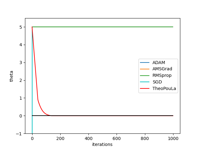
(a) default settings

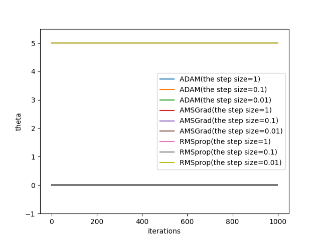
(b) different step sizes

Figure 1: Performance of SGD, Adam, AMSGrad, RMSProp and TH$\varepsilon$O POULA on an artificial example with the initial value $\theta_{0}=5.0$

Intuitively, the undesirable phenomenon occurs because, in the iterating rule (3), the denominator $\sqrt{V}_{n}$ excessively dominates the numerator $m_{n}$, causing the vanishing gradient problem in the presence of the superlinear gradient. On the contrary, SGD suffers from the exploding gradient problem. Moreover, Figure 1(b) highlights that the problematic behavior cannot be simply resolved by adjusting the learning rate within the Adam-type framework, while TH$\varepsilon$O POULA perform extremely well even in the presence of such violent non-linearities.

3 New Algorithm: TH$\varepsilon$O POULA

We propose a new stochastic optimization algorithm by combining ideas from taming methods specifically designed to approximate Langevin SDEs with a hybrid approach based on recent advances of polygonal Euler approximations. The latter is achieved by identifying a suitable boosting function (of order $\epsilon\ll 1$) to efficiently deal with the sparsity of (stochastic) gradients of neural networks. In other words, the novelty of our algorithm is to utilize a taming function and a boosting function, rather than designing a new $V_{n}$ as in Adam-type optimizers.

We proceed with the necessary preliminary information, main assumptions and formal introduction of the new algorithm.

3.1 Preliminaries and Assumptions

Let $(\Omega,\mathcal{F},P)$ be a probability space. We denote by $\mathbb{E}[X]$ the expectation of a random variable $X$. Fix an integer $k\geq 1$. For an $\mathbb{R}^{k}$-valued random variable $X$, its law on $\mathcal{B}(\mathbb{R}^{k})$, i.e. the Borel sigma-algebra of $\mathbb{R}^{k}$, is denoted by $\mathcal{L}(X)$. Scalar product is denoted by $\langle\cdot,\cdot\rangle$, with $|\cdot|$ standing for the corresponding norm (where the dimension of the space may vary depending on the context). For any integer $q\geq 1$, let $\mathcal{P}(\mathbb{R}^{q})$ denote the set of probability measures on $\mathcal{B}(\mathbb{R}^{q})$. For $\mu,\nu\in\mathcal{P}(\mathbb{R}^{k})$, let $\mathcal{C}(\mu,\nu)$ denote the set of probability measures $\zeta$ on $\mathcal{B}(\mathbb{R}^{2k})$ such that its respective marginals are $\mu,\nu$. For two probability measures $\mu$ and $\nu$, the Wasserstein distance of order $p\geq 1$ is defined as

$${W}_{p}(\mu,\nu):=\inf_{\zeta\in\mathcal{C}(\mu,\nu)}\left(\int_{\mathbb{R}^{k}}\int_{\mathbb{R}^{k}}|\theta-\theta^{\prime}|^{p}\zeta(\mathrm{d}\theta\mathrm{d}\theta^{\prime})\right)^{1/p},\ \mu,\nu\in\mathcal{P}(\mathbb{R}^{k}).$$ (4)

Let $(X_{n})_{n\in\mathbb{N}}$ be a sequence of i.i.d. $\mathbb{R}^{m}$-valued random variables generating the filtration $(\mathcal{G}_{n})_{n\in\mathbb{N}}$ and $(\xi_{n})_{n\in\mathbb{N}}$ be an $\mathbb{R}^{d}$-valued Gaussian process with independent components.

Let $F:\mathbb{R}^{d}\times\mathbb{R}^{m}\rightarrow\mathbb{R}^{d}$ be continuously differentiable function such that $\mathbb{E}[F(\theta,X_{0})]<\infty$ for any $\theta\in\mathbb{R}^{d}$. We consider the following optimization problem

$$\min_{\theta}u(\theta) = \min_{\theta}\bigg{(}\mathbb{E}[F(\theta,X_{0})]+\frac{\eta}{2(r+1)}|\theta|^{2(r+1)}\bigg{)}$$ (5)

where $\theta\in\mathbb{R}^{d}$, $\eta\in(0,1)$ is the regularization parameter and $r\geq\frac{q}{2}+1$. In the context of fine tuning of neural networks, $F$ represents the loss function for the task at hand and $\theta$ denotes the vector of the neural network’s parameters. Note that the regularization term, $\frac{\eta}{2(r+1)}|\theta|^{2(r+1)}$, is added in order to guarantee that the dissipativity property holds, since it is essential for the convergence analysis.

Remark 3.1.

For the reader who prefers to consider the optimization problem without the regularization term, i.e. with $\eta=0$, the dissipative condition (B.1) has to be additionally assumed as in the literature [Raginsky et al., 2017, Xu et al., 2018, Erdogdu et al., 2018]. Then, the same analysis can be applied to obtain our main results without any additional effort. However, it is yet to be proven theoretically that such an assumption holds in general for neural networks and thus it becomes a case-by-case investigation. In other words, we present here the formal theoretical statement with the appropriate regularization term which covers all of these cases.

In particular, $r$ depends on the neural network’s structure, whereas $q$ is described in Assumption 3.1. Consequently, the stochastic gradient with the regularization term is given by

$$H(\theta,x):=G(\theta,x)+\eta\theta|\theta|^{2r}$$

where $G(\theta,x):=\nabla_{\theta}F(\theta,x)$ for all $x\in\mathbb{R}^{m}$, $\theta\in\mathbb{R}^{d}$ and $\eta=0$ if dissipativity holds for $G$.

We introduce our main assumptions. The first requirement is that $G$ is locally Lipschitz continuous.

Assumption 3.1.

There exists positive constant $L_{1}$, $\rho$ and $q\geq 1$ such that

$$|G(\theta,x)-G(\theta^{\prime},x)|\leq L_{1}(1+|x|)^{\rho}(1+|\theta|+|\theta^{\prime}|)^{q-1}|\theta-\theta^{\prime}|.$$

for all $x\in\mathbb{R}^{m}$ and $\theta,\theta^{\prime}\in\mathbb{R}^{d}$. Moreover, $h(\theta):=\mathbb{E}[H(\theta,X_{0})]$ for every $\theta\in\mathbb{R}^{d}$.

Further, conditions on the initial value $\theta_{0}$ and data process $(X_{n})_{n\in\mathbb{N}}$ are imposed as it is common to use weight initialization using the uniform or normal distribution, Assumption 3.2 is mild.

Assumption 3.2.

The process $(X_{n})_{n\in\mathbb{N}}$ is a sequence of i.i.d. random variables with $\mathbb{E}[|X_{0}|^{16\rho(2r+1)}]<\infty$ where $\rho$ is given in Assumption 3.1. In addition, the initial condition is such that $\mathbb{E}[|\theta_{0}|^{16(2r+1)}]<\infty$.

We refer to Appendix B for further remarks and key observations regarding the consequences of Assumptions 3.1 and 3.2. We conduct the convergence analysis of TH$\varepsilon$O POULA by employing elements of the theory of Langevin SDEs. It is shown that, under mild conditions (satisfied by Assumptions 3.1 and 3.2), the so-called (overdamped) Langevin SDE, which is given by

$${\rm d}Z_{t}=-h(Z_{t}){\rm d}t+\sqrt{2\beta^{-1}}{\rm d}B_{t},\quad t>0,$$ (6)

where $h=\nabla u$ with a (possibly random) initial condition $\theta_{0}$ and with $(B_{t})_{t\geq 0}$ denoting a $d$-dimensional Brownian motion, admits a unique invariant measure $\pi_{\beta}(dz)\propto\exp(-\beta u(z))$. Thus, for a sufficiently large $\beta$, $\pi_{\beta}$ concentrates around the minimizers of (5).

3.2 Mechanism of TH$\varepsilon$O POULA

We introduce the mechanism of TH$\varepsilon$O POULA, which iterately updates as follows:

$$\theta_{0}^{\lambda}:=\theta_{0},\qquad\theta_{n+1}^{\lambda}:=\theta_{n}^{\lambda}-\lambda H_{\lambda,c}(\theta_{n}^{\lambda},X_{n+1})+\sqrt{2\lambda\beta^{-1}}\xi_{n+1},\quad n\in\mathbb{N},$$ (7)

where $H_{\lambda,c}:=(H_{\lambda,c}^{(1)}(\theta,x),\cdots,H_{\lambda,c}^{(d)}(\theta,x))^{T}$ is given by

$$H_{\lambda,c}^{(i)}(\theta,x)=\frac{G^{(i)}(\theta,x)}{\underbrace{1+\sqrt{\lambda}|G^{(i)}(\theta,x)|}_{\mbox{taming function}}}\bigg{(}\underbrace{1+\frac{\sqrt{\lambda}}{\varepsilon+|G^{(i)}(\theta,x)|}}_{\mbox{boosting function}}\bigg{)}+\underbrace{\eta\frac{\theta^{(i)}|\theta|^{2r}}{1+\sqrt{\lambda}|\theta|^{2r}}}_{\mbox{regularization term}},$$ (8)

and $\{\xi_{n}\}_{n\geq 1}$ is a sequence of independent standard $d$-dimensional Gaussian random variables. Note that the taming and boosting functions are defined in (8).

TH$\varepsilon$O POULA has several distinct features over the existing optimization methods in the literature. We give an intuitive explanation as to how these features are complementarily harmonized to improve the performance of the algorithm, and to handle the exploding and vanishing gradient problems of neural networks. For simplicity, we omit the regularization term, that is, $\eta=0$, and the noise term, $\sqrt{2\lambda\beta^{-1}}\xi_{n+1}$, throughout the exposition. Also, we refer to $\lambda$ as the learning rate and $|\Delta\theta_{n}^{\lambda}|:=\frac{|G^{(i)}(\theta_{n}^{\lambda},X_{n+1})|}{1+\sqrt{\lambda}|G^{(i)}(\theta_{n}^{\lambda},X_{n+1})|}\bigg{(}1+\frac{\sqrt{\lambda}}{\varepsilon+|G^{(i)}(\theta_{n}^{\lambda},X_{n+1})|}\bigg{)}$ as the stepsize by the convention in Kingma and Ba [2015].

Firstly, the new algorithm utilizes the taming function to control the super-linearly growing gradient. In a region where the loss function is steep and narrow (the gradient is huge), it is ideal for the optimizer to take a small stepsize. This is effectively achieved since the growth of the taming function is proportional to $G$, but the boosting is close to one when the gradient is huge. The effectiveness of the taming function is confirmed in the motivating example in Section 2. Note that the taming function is applied element-wise to scale the effective element-wise learning rate in contrast to TUSLA of Lovas et al. [2020]. This significantly improves the performance of our new algorithm in solving high-dimensional optimization problems such as the fine tuning of neural network models.

Secondly, we have designed the boosting function to accelerate training speed and prevent the vanishing gradient problem. When the current parameter is located in a region where the loss function is flat (the gradient is small), it is desirable for the optimizer to take a large stepsize. As the gradient gets smaller, the boosting function increases the stepsize of TH$\varepsilon$O POULA by up to $\sqrt{\lambda}/\varepsilon$, whereas the taming function’s contribution decreases. As a result, TH$\varepsilon$O POULA takes a larger stepsize. In other words, TH$\varepsilon$O POULA takes a desirable stepsize depending on the magnitude of the gradient. Most importantly, the taming and boosting functions do not interfere with each other in any adverse way. On the contrary, they complement each other in a harmonious way that is evident from our simulation results.

Thirdly, TH$\varepsilon$O POULA is quickly converted from adaptive learning rate methods to SGD. In the early training phase, TH$\varepsilon$O POULA certainly behaviors like adaptive learning rate methods. Then, when the current position is approaching an optimal solution where $|G^{(i)}|$s are close to zero, the movement of TH$\varepsilon$O POULA is similar to SGD with a learning rate $(1+\sqrt{\lambda}/\varepsilon)$. Consequently, TH$\varepsilon$O POULA simultaneously attains two favorable features of fast training in adaptive learning rate methods and good generalization in SGD. The switching from adaptive learning rates to SGD has been also investigated by different strategies in Luo et al. [2019] and Keskar and Socher [2017].

Lastly, a scaled Gaussian noise, $\sqrt{2\lambda\beta^{-1}}\xi_{n+1}$, is added as a consequence of the discretization of the Langevin SDE. The term is essential to prove the convergence property of TH$\varepsilon$O POULA. Adding properly scaled Gaussian noise allows the new algorithm to escape local minima in a similar manner to the standard SGLD method, see Raginsky et al. [2017].

3.3 Convergence Analysis

We present in this section the main convergence results of TH$\varepsilon$O POULA to $\pi_{\beta}$ in Wasserstein-1 and Wasserstein-2 distances as defined in (4). The convergence is guaranteed when the step size is less than $\lambda_{\max}$, which is given by

$$\lambda_{\max}=\min\bigg{\{}\frac{1}{4\eta^{2}},\frac{1}{2^{14}\eta^{2}({}_{8l}\mathcal{C}_{4l})^{2}}\bigg{\}}.$$ (9)

where ${}_{n}\mathcal{C}_{k}$ is the binomial coefficient ‘$n$ choose $k$’ and $l=2r+1$. Note that the step size restriction causes no issues a $\eta$ is typically very small ($\eta\ll 1$). Moreover, let $T:=1/\lambda$.

Theorem 3.1 and Corollary 3.1 state the non-asymptotic (upper) bounds between $\mathcal{L}\left(\theta_{n}^{\lambda}\right)$ and $\pi_{\beta}$. An overview of the proofs of our main results can be found in Appendix C.

Theorem 3.1.

Let Assumptions 3.1 and 3.2 hold. Then, for every $0<\lambda\leq\lambda_{\max}$ and $n\in\mathbb{N}$, we have

$$W_{1}\left(\mathcal{L}\left(\theta_{n}^{\lambda}\right),\pi_{\beta}\right)\leq M_{1}\sqrt{\lambda}+M_{2}e^{-\dot{c}\lambda n},$$

where $\dot{c}$, $M_{1}$ and $M_{2}$ are constants independent of $n$ and $\lambda$. The explicit form of $\dot{c}$, $M_{1}$ and $M_{2}$ are given in Table 5.

Corollary 3.1.

Let Assumptions 3.1 and 3.2 hold. Then, for every $0<\lambda\leq\lambda_{max}$ and $n\in\mathbb{N}$, we have

$$W_{2}\left(\mathcal{L}\left(\theta_{n}^{\lambda}\right),\pi_{\beta}\right)\leq M_{3}\sqrt{\lambda}+z_{2}\lambda^{\frac{1}{4}}+M_{4}e^{-\dot{c}\lambda n},$$

where $\dot{c}$, $z_{2}$, $M_{3}$ and $M_{4}$ are constants independent of $n$ and $\lambda$. The explicit form of $\dot{c}$, $z_{2}$, $M_{3}$ and $M_{4}$ are given in Table 5.

We are now concerned with the expected excess risk of TH$\varepsilon$O POULA generated by (7), so called the optimization error of $\theta_{n}^{\lambda}$, defined as

$$\mathbb{E}[u(\theta_{n}^{\lambda})]-u(\theta^{*})$$ (10)

where $\theta^{*}:=\arg\min_{\theta\in\mathbb{R}^{d}}u(\theta)$. To derive the bound of the expected excess risk, it is again decomposed into two parts; $\mathbb{E}[u(\theta_{n}^{\lambda})]-\mathbb{E}[u(\theta_{\infty})]$ and $\mathbb{E}[u(\theta_{\infty})]-u(\theta^{*})$. Here, $\theta_{\infty}$ follows the invariant distribution $\pi_{\beta}$. The following theorem describes the bound of the expected excess risk of TH$\varepsilon$O POULA.

Theorem 3.2.

Let Assumptions 3.1 and 3.2 hold. For any $n\in\mathbb{N}$, the expected excess risk of the $n$-th iterate of TH$\varepsilon$O POULA (7) is upper bounded by

$$\mathbb{E}[u(\theta_{n}^{\lambda})]-u(\theta^{*})\leq M_{5}W_{2}(\mathcal{L}(\theta_{n}^{\lambda},\pi_{\beta}))+\frac{1}{\beta}\bigg{[}\frac{d}{2}\log\bigg{(}\frac{Ke}{A}\bigg{(}\frac{B}{d}\beta+1\bigg{)}\bigg{)}+\log 2\bigg{]}$$

where $W_{2}(\mathcal{L}(\theta_{n}^{\lambda}),\pi_{\beta})$ is given in Corollary 3.1 and $A$, $B$ are given in Remark B.2. and $M_{5}$, $K$ are given in Table 5. All the constatns are independent of $n$ and $\lambda$.

3.4 Averaged TH$\varepsilon$O POULA

One notes that Theorem 3.1 implies that TH$\varepsilon$O POULA converges, under suitable decreasing step size regmine, to the invariant measure $\pi_{\beta}$ and thus its performance can be further improved by averaging. It is achieved by averaging of trajectories of the parameters after a user-specified trigger $K$, $\frac{1}{n-K+1}\sum_{i=K}^{n}\theta_{i}^{\lambda}$, instead of the last updated parameter $\theta_{n}^{\lambda}$ [Polyak and Juditsky, 1992]. In particular, we use a trigger strategy which starts the averaging when no improvement in the validation metric is seen for a patience number of epochs. For our experiments, we set the patience number to $5$.

Our experiments show that averaged TH$\varepsilon$O POULA performs better than the other stochastic optimization methods for language modeling tasks. Moreover, while a learning rate decay, which requires additional tuning effort, has to be applied for the other optimizers to obtain their best performance, averaged TH$\varepsilon$O POULA uses a constant learning rate, which is another practical benefit of our newly proposed algorithm.

4 Emprical performance on real data sets

This section examines the performance of TH$\varepsilon$O POULA on real data sets by comparing it with those of other stochastic optimization algorithms including Adam (Kingma and Ba [2015]), AdaBelief (Zhuang et al. [2020]), AdamP (Heo et al. [2021]), AdaBound (Luo et al. [2019]), AMSGrad (Reddi et al. [2018]), RMSProp (Tieleman and Hinton [2012]), SGD (with momentum) and ASGD (Merity et al. [2018]). We conduct the following deep learning experiments: image classficiation on CIFAR-10 (Krizhevsky et al. ) and CIFAR-100 (Krizhevsk [2009]) and language modeling on Penn Treebank (Marcus et al. [1999]). Each experiment is run three times to compute the mean and standard deviation of the best accuracy on the test dataset. We provide details of the experiments including learning curves and hyperparameter settings in Appendix E.

For our experiments, we consider $\eta=0$ in (5). This is justified by the fact that some form of dissipativity may exist for specific problems such as the one considered here, although this has not been verified theoretical so far.

Image classification

We replicate the experiments of VGG11 (Simonya and Zisserman [2015]), ResNet34 (Ioffe and Szegedy [2016]) and DenseNet121 (Huang et al. [2017]) on CIFAR-10 and CIFAR-100 in the official implementation of Zhuang et al. [2020]. They provide a reliable baseline of the experiments by comparing the performance of various stochastic optimizers with extensive hyperparameter search. We search the optimal hyperparameters for TH$\varepsilon$O POULA among $\lambda=\{1,0.5,0.1,0.05,0.01\}$ and $\varepsilon=\{1,0.1,0.01\}$. $\beta$ is set to $10^{12}$ across all the experiments.

Table 2 shows the test accuracy for VGG11, ResNet34 and DenseNet121 on CIFAR-10 and CIFAR-100. As reported in Table 2, our algorithm achieves the highest accuracy except for VGG11 on CIFAR-10 and significantly outperforms the other optimizers across all the experiments. In particular, even TH$\varepsilon$O POULA with the second best hyperparameter is comparable to AdaBelief and outperforms the other methods, validating that the solutions found by TH$\varepsilon$O POULA yield good generalization performance. Also, the improvement of our algorithm is increasingly prominent as the models and datasets are more complicated and large-scale.

Table 2: Mean and standard deviation of the best accuracy for VGG11, ResNet34 and DenseNet121 on CIFAR10. TH$\varepsilon$OPOULA^† and TH$\varepsilon$OPOULA^∗ represent the performances of TH$\varepsilon$O POULA with the best and second best hyperparameters, respectively.

dataset	CIFAR-10			CIFAR-100
model	VGG	ResNet	DenseNet	VGG	ResNet	DenseNet
TH$\varepsilon$O POULA†	92.10	95.43	95.66	70.31	77.53	79.90
	(0.0231)	(0.095)	(0.066)	(0.117)	(0.144)	(0.133)
TH$\varepsilon$O POULA∗	91.92	94.92	95.59	70.24	76.88	78.76
	(0.119)	(0.076)	(0.067)	(0.227)	(0.536)	(0.269)
AdaBelief	92.17	95.29	95.58	69.50	77.33	79.12
(baseline)	(0.035)	(0.196)	(0.095)	(0.111)	(0.172)	(0.382)
Adam	90.79	93.11	93.21	67.30	73.02	74.03
	(0.075)	(0.184)	(0.240)	(0.137)	(0.231)	(0.334)
AdamP	91.68	95.18	95.17	69.41	76.14	77.58
	(0.162)	(0.116)	(0.079)	(0.297)	(0.347)	(0.091)
AdaBound	91.81	94.83	95.05	68.61	76.27	77.56
	(0.272)	(0.131)	(0.176)	(0.312)	(0.256)	(0.120)
AMSGrad	91.24	93.76	93.74	67.71	73.51	74.50
	(0.115)	(0.108)	(0.236)	(0.291)	(0.692)	(0.416)
RMSProp	90.82	93.06	92.89	65.45	71.79	71.75
	(0.201)	(0.120)	(0.310)	(0.394)	(0.287)	(0.632)
SGD	90.73	94.61	94.46	67.78	77.16	78.95
	(0.090)	(0.280)	(0.159)	(0.320)	(0.214)	(0.312)

Language modeling

We perform language modeling over the Penn Treebank (PTB) with AWD-LSTMs of Merity et al. [2018]. It is reported that Non-monotonically Triggered ASGD (NT-ASGD) achieves state-of-the-art performance for the language modeling task with AWD-LSTMs. Motivated by this observation, we consider averaged TH$\varepsilon$O POULA for the experiment. Due to a limited computation budget, we only test ASGD and AdaBelief rather than investigating all the optimizers in this experiment .

For a fair comparison, the averaging scheme has also been applied to AdaBelief, but we have found that it does not improve the performance of AdaBelief. Instead, AdaBelief uses a development-based learning rate decay, which decreases the learning rate by a constant factor if the model does not attain a new best value for multiple epochs. For ASGD and TH$\varepsilon$O POULA, a constant learning rate is used without a learning rate decay. In order to compare with the baseline, we apply gradient clipping of $0.25$ to all optimizers. See Appendix E for more information.

Table 3: Test perplexity for language modeling tasks on PTB. Lower is better.

# of layers	1-layer	2-layer	3-layer
TH$\varepsilon$O POULA	82.75	67.15	61.07
	(0.209)	(0.126)	(0.161)
ASGD	82.85	67.53	61.60
(baseline)	(0.308)	(0.171)	(0.094)
AdaBelief	84.46	67.34	61.52
	(0.272)	(0.496)	(0.302)

Table 3 shows that TH$\varepsilon$O POULA attains the lower test perplexity against the baselines for AWD-LSTM with one, two and three layers, confirming the superiority of our algorithm. AdaBelief shows a comparable performance with ASGD for 2-layer and 3-layer models.

Our experimental results show that TH$\varepsilon$O POULA achieves higher accuracy than AdaBelief (known as the state-of-the-art algorithm for many deep learning tasks) on image classification and language modeling tasks for various deep learning models. Furthermore, it is easier to tune parameters of TH$\varepsilon$O POULA since the number of hyperparmeters for TH$\varepsilon$O POULA is less than that of Adam-type optimizers.

5 Conclusion and Discussion

This paper begins with an example which illustrates that local Lipschitz continuous gradients can cause serious convergence issues for popular adaptive optimization methods. Such issues manifest themselves as vanishing/exploding gradient phenomena. It proceeds by proposing a novel optimization framework, which is suitable for the fine tuning of neural network models by combining elements of the theory of Langevin SDEs, tamed algorithms and carefully designed boosting functions that handle sparse and super-linearly growing gradients. Further, a detailed convergence analysis of the newly proposed algorithm TH$\varepsilon$O POULA is provided along with full theoretical guarantees for obtaining the best known convergence rates. Our experiments confirm that TH$\varepsilon$O POULA outperforms other popular stochastic optimization methods.

We believe that there is much room for improvement of our novel framework. For example, the improved performance can be further achieved by identifying more efficient taming and boosting functions, which demonstrates the potential of our framework.

Appendix

Appendix A Details of the Experiment in Section 2

This section provides the necessary theoretical details of the experiment in Section 2. We continue to consider the optimization problem (2). One calculates that

$$u(\theta)=\left\{\begin{array}[]{ll}&\theta^{30}+\frac{7}{4}\theta^{2},\quad|\theta|\leq 1,\\ &\theta^{30}+\frac{7}{4}(2|\theta|-1),\quad|\theta|>1\end{array}\right.$$

and

$$u^{\prime}(\theta)=\left\{\begin{array}[]{ll}&30\theta^{29}+\frac{7}{2}\theta,\quad|\theta|\leq 1,\\ &30\theta^{29}+\frac{7}{2}sgn(\theta),\quad|\theta|>1.\end{array}\right.$$

Note that $u(\theta)$ and $u^{\prime}(\theta)$ are continuous since $u(1)=\lim_{\theta\downarrow 1}u(\theta)=\frac{11}{4}$, $u(-1)=\lim_{\theta\uparrow-1}=\frac{11}{4}$, $u^{\prime}(1)=\lim_{\theta\downarrow-1}u^{\prime}(1)=\frac{67}{2}$ and $u^{\prime}(-1)=\lim_{\theta\uparrow 1}u^{\prime}(-1)=-\frac{67}{2}$. Therefore, the minimum value is attained at $\theta=0$.

To show that $G$ is locally Lipschitz continuous, we check that for $|\theta|,|\theta^{\prime}|>1$ and $x\in\mathbb{R}^{d}$,

$$|G(\theta,x)-G(\theta^{\prime},x)| \leq (2+2\mathbbm{1}_{x\leq 1})|sgn(\theta)-sgn(\theta^{\prime})|+30|\theta^{29}-\theta^{\prime 29}|$$

$$\leq 34(1+|\theta|+|\theta^{\prime}|)^{28}|\theta-\theta^{\prime}|.$$

For $|\theta|,|\theta|\leq 1$, we have

$$|G(\theta,x)-G(\theta^{\prime},x)| \leq (2+2\mathbbm{1}_{x\leq 1})|\theta-\theta^{\prime}|+30|\theta^{29}-\theta^{\prime 29}|$$

$$\leq 34(1+|\theta|+|\theta^{\prime}|)^{28}|\theta-\theta^{\prime}|.$$

For $|\theta|\leq 1$, $|\theta|>1$, we obtain

$$|G(\theta,x)-G(\theta^{\prime},x)| \leq (2+2\mathbbm{1}_{x\leq 1})|\theta-sgn(\theta^{\prime})|+30|\theta^{29}-\theta^{\prime 29}|$$

$$\leq (2+2\mathbbm{1}_{x\leq 1})|\theta-\theta^{\prime}|+30|\theta^{29}-\theta^{\prime 29}|$$

$$\leq 34(1+|\theta|+|\theta^{\prime}|)^{28}|\theta-\theta^{\prime}|$$

where the second inequality follows from the following relations

$$\theta-\theta^{\prime}\leq\theta-1\leq 0,\quad\mbox{for }\theta^{\prime}>1,$$

$$0\leq\theta+1\leq\theta-\theta^{\prime},\quad\mbox{for }\theta^{\prime}<-1.$$

Appendix B Key Observations from Assumption 3.1 and 3.2

This section introduces some useful general results, that can be obtained from Assumption 3.1 and 3.2. Note that some of the below observations can be also found in Zhang et al. [2019] and Lovas et al. [2020]. However, to make our paper self-contained, we record all the results which are necessary for the convergence analysis.

Remark B.1.

From Assumption 3.1, one observes that for all $\theta\in\mathbb{R}^{d}$ and $x\in\mathbb{R}^{m}$

$$|G(\theta,x)|\leq K(x)(1+|\theta|^{q}),$$

where $K(x)=2^{q}(L_{1}(1+|x|)^{\rho}+|G(0,x)|)$.

Remark B.2.

From Assumptions  3.1 and 3.2, one obtains that

$${\langle\theta,\,h(\theta)\rangle}={\langle\theta,\,\mathbb{E}G(\theta,X_{0})\rangle}+{\langle\theta,\,\eta\theta|\theta|^{2r}\rangle}\geq\eta|\theta|^{2r+2}-\mathbb{E}[K(X_{0})]|\theta|(1+|\theta|^{q}).$$

Furthermore, for $A=\mathbb{E}[K(X_{0})]$ and $B=(3\mathbb{E}[K(X_{0})])^{q+2}\eta^{-q-1}$, it holds that

$${\langle\theta,\,h(\theta)\rangle}\geq A|\theta|^{2}-B.$$ (B.1)

Proposition B.1.

(Lovas et al. [2020]) Let Assumptions  3.1 and  3.2 hold. Then, for every $\theta$, $\theta^{\prime}\in\mathbb{R}^{d}$,

$${\langle\theta-\theta^{\prime},\,h(\theta)-h(\theta^{\prime})\rangle}\geq-a|\theta-\theta^{\prime}|^{2},$$

where $a=L_{1}\mathbb{E}[(1+|X_{0}|)^{\rho}](1+2|R|)^{q-1}$ and $R$ is given by

$$R=\max\bigg{\{}\bigg{(}\frac{2^{3(q-1)+1}L_{1}\mathbb{E}[(1+|X_{0}|)^{\rho}]}{\eta}\bigg{)}^{\frac{1}{2r-1}},\bigg{(}\frac{2^{q}L_{1}\mathbb{E}[(1+|X_{0}|)^{\rho}]}{\eta}\bigg{)}^{\frac{1}{2r}}\bigg{\}}.$$

Proposition B.2.

(Lovas et al. [2020]) Let Assumptions 3.1 and 3.2 hold. Then, one obtains that

$$|H(\theta,x)-H(\theta^{\prime},x)|\leq L(1+|x|)^{\rho}(1+|\theta|+|\theta^{\prime}|)^{l}|\theta-\theta^{\prime}|,\qquad\mbox{ for all }\theta\in\mathbb{R}^{d}\mbox{ and }x\in\mathbb{R}^{m},$$

where $L=L_{1}+8r\eta$ and $l=2r+1$.

Remark B.3.

From Assumption 3.1 and the definition of $H$ and $H_{\lambda,c}$, one obtains that for $\theta\in\mathbb{R}^{d}$, $x\in\mathbb{R}^{m}$ and $i=1,2,\cdots,d$,

$$|H^{(i)}(\theta,x)-H_{\lambda,c}^{(i)}(\theta,x)| \leq \bigg{|}G^{(i)}(\theta,x)-\frac{G^{(i)}(\theta,x)}{1+\sqrt{\lambda}|G^{(i)}(\theta,x)|}\bigg{(}1+\frac{\sqrt{\lambda}}{\epsilon+|G^{(i)}(\theta,x)|}\bigg{)}\bigg{|}$$

$$+ \bigg{|}\eta\theta^{(i)}|\theta|^{2r}-\eta\frac{\theta^{(i)}|\theta|^{2r}}{1+\sqrt{\lambda}|\theta|^{2r}}\bigg{|}$$

$$\leq |G^{(i)}(\theta,x)|\frac{\sqrt{\lambda}|G^{(i)}(\theta,x)|}{1+\sqrt{\lambda}|G^{(i)}(\theta,x)|}+\frac{\sqrt{\lambda}|G^{(i)}(\theta,x)|}{(1+\sqrt{\lambda}|G^{(i)}(\theta,x)|)(\epsilon+|G^{(i)}(\theta,x)|)}$$

$$+ \eta|\theta^{(i)}||\theta|^{2r}\bigg{|}\frac{\sqrt{\lambda}|\theta|^{2r}}{1+\sqrt{\lambda}|\theta|^{2r}}\bigg{|}$$

$$\leq \sqrt{\lambda}|G^{(i)}(\theta,x)|^{2}+\sqrt{\lambda}+\sqrt{\lambda}\eta|\theta^{(i)}||\theta|^{4r}$$

which implies that

$$|H(\theta,x)-H_{\lambda,c}(\theta,x)|^{2} = \sum_{i=1}^{d}\bigg{[}\sqrt{\lambda}|G^{(i)}(\theta,x)|^{2}+\sqrt{\lambda}+\sqrt{\lambda}\eta|\theta^{(i)}||\theta|^{4r}\bigg{]}^{2}$$

$$\leq 3\lambda\sum_{i=1}^{d}\bigg{[}|G^{(i)}(\theta,x)|^{4}+1+\eta^{2}|\theta^{(i)}|^{2}|\theta|^{8r}\bigg{]}$$

$$\leq 3\lambda\bigg{[}\bigg{(}\sum_{i=1}^{d}|G^{(i)}(\theta,x)|^{2}\bigg{)}^{2}+d+\eta^{2}|\theta|^{8r+2}\bigg{]}$$

$$\leq 3\lambda\bigg{[}|G(\theta,x)|^{4}+d+\eta^{2}|\theta|^{8r+2}\bigg{]}$$

$$\leq 3\lambda\bigg{[}8|K(x)|^{4}(1+|\theta|^{4q})+d+\eta^{2}|\theta|^{8r+2}\bigg{]}$$

Remark B.4.

From Assumption 3.1 and the definition of $H$ and $H_{\lambda,c}$, one calculates that for all $\theta\in\mathbb{R}^{d}$ and $x\in\mathbb{R}^{m}$,

$$|H(\theta,x)|^{2}=|G(\theta,x)+\eta\theta|\theta|^{2r}|^{2} \leq 2|G(\theta,x)|^{2}+2\eta^{2}|\theta|^{4r+2}$$

$$\leq 4|K(x)|^{2}(1+|\theta|^{2q})+2\eta^{2}|\theta|^{4r+2}$$

and

$$|H_{\lambda,c}(\theta,x)|^{2} = \sum_{i=1}^{d}\bigg{[}\frac{G^{(i)}(\theta,x)}{1+\sqrt{\lambda}|G^{(i)}(\theta,x)|}\bigg{(}1+\frac{\sqrt{\lambda}}{\epsilon+|G^{(i)}(\theta,x)|}\bigg{)}+\eta\frac{\theta^{(i)}|\theta|^{2r}}{1+\sqrt{\lambda}|\theta|^{2r}}\bigg{]}^{2}$$

$$\leq \sum_{i=1}^{d}\bigg{[}\frac{|G^{(i)}(\theta,x)|}{1+\sqrt{\lambda}|G^{(i)}(\theta,x)|}+\frac{\sqrt{\lambda}|G^{(i)}(\theta,x)|}{(1+\sqrt{\lambda}|G^{(i)}(\theta,x)|)(\epsilon+|G^{(i)}(\theta,x)|)}+\eta\frac{|\theta^{(i)|}|\theta|^{2r}}{1+\sqrt{\lambda}|\theta|^{2r}}\bigg{]}^{2}$$

$$\leq \sum_{i=1}^{d}\bigg{(}|G^{(i)}(\theta,x)|+\sqrt{\lambda}+\eta|\theta^{(i)}||\theta|^{2r}\bigg{)}^{2}$$

$$\leq 3\sum_{i=1}^{d}\bigg{(}|G^{(i)}(\theta,x)|^{2}+\lambda+\eta^{2}|\theta^{(i)}|^{2}|\theta|^{4r}\bigg{)}$$

$$\leq 3|G(\theta,x)|^{2}+3\lambda d+3\eta^{2}|\theta|^{4r+2}$$

$$\leq 6|K(x)|^{2}(1+|\theta|^{2q})+3\lambda d+3\eta^{2}|\theta|^{4r+2}.$$

Appendix C Overview of the Proofs

This section provides an overview of the proofs of our main results. We begin by introducing suitable Lyapunov functions and auxiliary processes to analyze the convergence of our newly introduced algorithm. For each $m\geq 1$, define the Lyapunov function $V_{m}$ by

$$V_{m}(\theta):=(1+|\theta|^{2})^{\frac{m}{2}},\quad\theta\in\mathbb{R}^{d}$$ (C.1)

and similarly $v_{m}(x)=(1+x^{2})^{\frac{m}{2}}$ for any real $x\geq 0$. Both functions are continuously differentiable and $\lim_{|\theta|\rightarrow\infty}\nabla V_{m}(\theta)/V_{m}(\theta)=0$. Also, define $Z_{t}^{\lambda}=Z_{\lambda t}$, which is the time-changed Lagevin dynamics governed by

$$dZ_{t}^{\lambda}=-\lambda h(Z_{t}^{\lambda})dt+\sqrt{2\beta^{-1}\lambda}d\tilde{B}_{t}^{\lambda}$$ (C.2)

where $\tilde{B}_{t}^{\lambda}=B_{\lambda t}/\sqrt{\lambda}$ is a Brownian motion.

We next define the continuous-time interpolation of the new algorithm, see (7), as

$$\mathrm{d}\bar{\theta}_{t}^{\lambda}=-\lambda H_{\lambda}\left(\bar{\theta}_{\lfloor t\rfloor}^{\lambda},X_{\lceil t\rceil}\right)\mathrm{d}t+\sqrt{2\lambda\beta^{-1}}\mathrm{d}\tilde{B}_{t}^{\lambda}$$ (C.3)

with initial condition $\bar{\theta}_{0}^{\lambda}=\theta^{\lambda}_{0}$. Henceforth, $\lfloor x\rfloor$ denotes the integer part of a positive real $x$ and $\lceil x\rceil=\lfloor x\rfloor+1$.

Remark C.1.

Due to the homogeneous nature of the coefficients of the continuous-time interpolation of TH$\varepsilon$O POULA (C.3) and when one selects a version of the driving Brownian motion such that it coincides with $\xi_{n}$ at grid points, it follows that the interpolated process (C.3) equals the process of TH$\varepsilon$O POULA (7) almost surely at grid points, i.e. $\bar{\theta}_{n}^{\lambda}=\theta_{n}^{\lambda}$ (a.s), $\forall n\in\mathbb{N}$.

Furthermore consider the continuous-time process $\zeta_{t}^{s,v,\lambda},t\geq s$ which is the solution to the SDE

$$\mathrm{d}\zeta_{t}^{s,v,\lambda}=-\lambda h\left(\zeta_{t}^{s,v,\lambda}\right)\mathrm{d}t+\sqrt{2\lambda\beta^{-1}}\mathrm{d}\tilde{B}_{t}^{\lambda}$$ (C.4)

with initial condition $\zeta_{s}^{s,v,\lambda}:=v,v\in\mathbb{R}^{d}$. Let us also define $T:=\frac{1}{\lambda}$, which allows us to create suitable subintervals on the positive real line in order to compare the behaviour of the aforementioned processes at each such interval.

Definition C.1.

Fix $k\in\mathbb{N}$ and define $\bar{\zeta}_{t}^{\lambda,k}:=\zeta_{t}^{kT,\bar{\theta}_{kT}^{\lambda},\lambda}$ where $\zeta_{t}^{kT,\bar{\theta}_{kT}^{\lambda},\lambda}$ is defined in (C.4).

To derive non-asymptotic (upper) bounds for $W_{1}\left(\mathcal{L}\left(\theta_{t}^{\lambda}\right),\pi_{\beta}\right)$ and $W_{2}\left(\mathcal{L}\left(\theta_{t}^{\lambda}\right),\pi_{\beta}\right)$, the following decomposition is used in terms of the auxiliary processes $\bar{\theta}_{t}^{\lambda}$, $\bar{\zeta}_{t}^{\lambda,n}$ and $Z_{t}^{\lambda}$ as follows:

$$W_{j}\left(\mathcal{L}\left(\theta_{t}^{\lambda}\right),\pi_{\beta}\right)\leq W_{j}\left(\mathcal{L}\left(\bar{\theta}_{t}^{\lambda}\right),\mathcal{L}\left(\bar{\zeta}_{t}^{\lambda,n}\right)\right)+W_{j}\left(\mathcal{L}\left(\bar{\zeta}_{t}^{\lambda,n}\right),\mathcal{L}\left(Z_{t}^{\lambda}\right)\right)+W_{j}\left(\mathcal{L}\left(Z_{t}^{\lambda}\right),\pi_{\beta}\right)$$

for $j=1,2$.

C.1 Primary estimates

We collect first the necessary estimates in order to obtain (upper) bounds for $W_{1}\left(\mathcal{L}\left(\theta_{t}^{\lambda}\right),\pi_{\beta}\right)$ and $W_{2}\left(\mathcal{L}\left(\theta_{t}^{\lambda}\right),\pi_{\beta}\right)$. All proofs of the lemmas in this section can be found in Appendix D. The following two lemmas provide, uniform in $n$, moment estimates of the process $(\theta_{n}^{\lambda})_{n\geq 1}$.

Lemma C.1.

Let Assumptions 3.1 and 3.2 hold. Then, there exist $M_{0}>0$ and $\lambda_{\max}$, which is defined in (9), such that for any $\lambda\in(0,\,\lambda_{\max})$ and any $n\in\mathbb{N}$,

$$\mathbb{E}|\theta_{n+1}^{\lambda}|^{2}\leq \bigg{(}1-\frac{\eta}{2}\sqrt{\lambda}\bigg{)}^{n}\mathbb{E}|\theta_{0}|^{2}+\bigg{[}5M_{0}^{2}+\frac{4\sqrt{\lambda_{\max}}d}{\eta}\bigg{(}\beta^{-1}+2+2\lambda_{\max}^{2}\bigg{)}$$

$$\phantom{\bigg{(}1-\frac{\eta}{2}\sqrt{\lambda}\bigg{)}^{n}\mathbb{E}|\theta_{0}|^{2}+\bigg{[}}+\frac{4(1+\lambda_{\max})\sqrt{d}M_{0}}{\eta}+4\eta M_{0}^{2}\sqrt{\lambda_{\max}}\bigg{]}$$

and, moreover,

$$\sup_{n}\mathbb{E}|\theta_{n+1}^{\lambda}|^{2}\leq \mathbb{E}|\theta_{0}|^{2}+\bigg{[}5M_{0}^{2}+\frac{4\sqrt{\lambda_{\max}}d}{\eta}\bigg{(}\beta^{-1}+2+2\lambda_{\max}^{2}\bigg{)}$$

$$\phantom{\mathbb{E}|\theta_{0}|^{2}+\bigg{[}}+\frac{4(1+\lambda_{\max})\sqrt{d}M_{0}}{\eta}+4\eta M_{0}^{2}\sqrt{\lambda_{\max}}\bigg{]}.$$

Lemma C.2.

Let Assumptions 3.1 and 3.2 hold. Then, there exist $M_{0}>0$ and $\lambda_{\max}$, which is defined in (9), such that for any $\lambda\in(0,\,\lambda_{\max})$, $n\in\mathbb{N}$, and $p\in[1,8(2r+1)]$,

$$\mathbb{E}|\theta_{n+1}^{\lambda}|^{2p}\leq(1-\eta^{2}\lambda)^{n}\mathbb{E}|\theta_{0}^{\lambda}|^{2p}+\frac{A_{p}}{\eta^{2}}$$

and

$$\sup_{n}\mathbb{E}|\theta_{n+1}^{\lambda}|^{2p}\leq\mathbb{E}|\theta_{0}^{\lambda}|^{2p}+\frac{A_{p}}{\eta^{2}}$$

where $A_{p}$ is given in Table 5.

Lemma C.3.

Let Assumptions 3.1 and  3.2 hold. Then, there exist $M_{0}>0$ and $\lambda_{\max}$, which is defined in (9), such that for any $\lambda\in(0,\,\lambda_{\max})$ and $n\in\mathbb{N}$,

$$\mathbb{E}[V_{4}(\bar{\theta}^{\lambda}_{nT})]\leq 2\mathbb{E}|\theta_{0}|^{4}+2+2\frac{A_{2}}{\eta^{2}}.$$

where $A_{2}$, i.e. $A_{p}$ for $p=2$, is given in Table 5.

Proof.

From the definition of the Lyapunov function and Remark C.1, we have

$$\mathbb{E}[V_{4}(\bar{\theta}^{\lambda}_{nT})] = \mathbb{E}[(1+|\bar{\theta}^{\lambda}_{nT}|^{2})^{2}]$$

$$\leq 2+2\mathbb{E}|\bar{\theta}^{\lambda}_{nT}|^{4}$$

$$\leq 2+2\mathbb{E}|\theta_{0}|^{4}+2\frac{A_{2}}{\eta^{2}}$$

∎

Moreover, the necassary moment bounds hold also for the auxiliary process $\{\bar{\zeta}_{t}^{\lambda,n}\}_{t\geq nT}$.

Lemma C.4.

(Lemma 3.5. of Chau et al. [2019]) Let Assumptions 3.1 and  3.2 hold. Then,

$$\mathbb{E}[V_{2}(\bar{\zeta}_{t}^{\lambda,n})] \leq \mathbb{E}[V_{2}(\theta_{0})]+\frac{\tilde{c}(2)}{\bar{c}(2)}+2(C_{X}\eta^{-1}+2M_{0}^{2}(2+\eta)+2d(\eta\beta)^{-1}\sqrt{\lambda_{\max}})+1,$$

$$\mathbb{E}[V_{4}(\bar{\zeta}_{t}^{\lambda,n})] \leq 2\mathbb{E}|\theta_{0}|^{4}+2+2\frac{A_{2}}{\eta^{2}}+\frac{\tilde{c}(4)}{\bar{c}(4)},$$

where $\bar{c}(p)$, $\tilde{c}(p)$ are given in Table 5.

Let $\mathcal{P}_{V_{2}}$ denote the subset of $\mathcal{P}(\mathbb{R}^{d})$ such that every $\mu\in\mathcal{P}_{V_{2}}$ satisfies $\int_{\mathbb{R}^{d}}V_{2}(\theta)\mu(d\theta)<\infty$. Moreover, let the following functional be considered

$$w_{1,2}(\mu,\nu):=\inf_{\zeta\in\mathcal{C}(\mu,\nu)}\int_{\mathbb{R}^{d}}\int_{\mathbb{R}^{d}}\left[1\wedge|\theta-\theta|^{\prime}\right]\left[\left(1+V_{2}(\theta)+V_{2}\left(\theta^{\prime}\right)\right)\zeta\left(\mathrm{d}\theta\mathrm{d}\theta^{\prime}\right)\right.$$ (C.5)

where $\mathcal{C}(\mu,\nu)$ is defined in (4). The following lemma states the contraction property of the Langevin SDE (C.2) in $w_{1,2}$, which yields the desired result for $W_{1}(\mathcal{L}(Z^{\lambda}_{n}),\pi_{\beta})$.

Lemma C.5.

(Proposition 3.14 of Chau et al. [2019]) Let $Z_{t}^{\prime},t\in\mathbb{R}_{+}$ be the solution of the Langevin SDE (6) with initial condition $Z_{0}^{\prime}=\theta^{\prime}_{0}$ which is independent of $\mathcal{G}_{\infty}$ and $\left|\theta^{\prime}_{0}\right|\in L^{2}.$ Then,

$$w_{1,2}\left(\mathcal{L}\left(Z_{t}^{\lambda}\right),\mathcal{L}\left(Z_{t}^{\prime}\right)\right)\leq\hat{c}e^{-\dot{c}t}w_{1,2}\left(\mathcal{L}\left(\theta_{0}\right),\mathcal{L}\left(\theta_{0}^{\prime}\right)\right)$$

where $w_{1,2}$ is defined in (C.5).

The following two Lemmas combined establish the required $W_{1}(\mathcal{L}(\bar{\theta}^{\lambda}_{t}),\mathcal{L}(Z^{\lambda}_{t}))$ estimate. One recalls first that for any $t>0$, there exists a unique integer $m$ such that $t\in[mT,(m+1)T)$.

Lemma C.6.

Let Assumptions 3.1 and 3.2 hold. Then, for $0<\lambda<\lambda_{max}$, one obtains

$$W_{2}\left(\mathcal{L}\left(\bar{\theta}_{t}^{\lambda}\right),\mathcal{L}\left(\bar{\zeta}_{t}^{\lambda,m}\right)\right)\leq\sqrt{\lambda}\sqrt{e^{3a}(C_{1}+C_{2}+C_{3})}$$

where $C_{1}$, $C_{2}$, $C_{3}$ are given explicitly in Table 5.

Lemma C.7.

Let Assumptions 3.1 and 3.2 hold. Then, for $0<\lambda<\lambda_{max}$, one obtains

$$W_{1}\left(\mathcal{L}\left(\bar{\zeta}_{t}^{\lambda,m}\right),\mathcal{L}\left(Z_{t}^{\lambda}\right)\right)\leq\sqrt{\lambda}z_{1}$$

where $z_{1}$ is given explicitly in Table 5.

Lemma C.8.

Let Assumptions  3.1 and  3.2 hold. Then, for $0<\lambda<\lambda_{max}$, one obtains

$$W_{2}\left(\mathcal{L}\left(\bar{\zeta}_{t}^{\lambda,m}\right),\mathcal{L}\left(Z_{t}^{\lambda}\right)\right)\leq\lambda^{\frac{1}{4}}z_{2}$$

where $z_{2}$ is given explicitly in Table 5.

C.2 Proofs of main results

It is assumed throughout the paper that the random variable $\theta_{0}$, $\mathcal{G}_{\infty}:=\sigma\left(\cup_{n\in\mathbb{N}}\mathcal{G}_{n}\right)$ and $(\xi_{n})_{n\in\mathbb{N}}$ are independent.

Proof of Theorem 3.1.

Observe that $W_{1}\left(\mathcal{L}\left(\theta_{n}^{\lambda}\right),\mathcal{L}\left(Z_{t}^{\lambda}\right)\right)$ is decomposed as follows:

$$W_{1}\left(\mathcal{L}\left(\theta_{n}^{\lambda}\right),\pi_{\beta}\right)\leq W_{1}\left(\mathcal{L}\left(\bar{\theta}_{n}^{\lambda}\right),\mathcal{L}\left(Z_{n}^{\lambda}\right)\right)+W_{1}\left(\mathcal{L}\left(Z_{n}^{\lambda}\right),\pi_{\beta}\right).$$

Note that there exists a unique integer $m$ such that $n\in[mT,(m+1)T)$. Thus, from the results of Lemma C.6 and C.7, the first term in the right-hand side is estimated

$$W_{1}\left(\mathcal{L}\left(\bar{\theta}_{n}^{\lambda}\right),\mathcal{L}\left(Z_{n}^{\lambda}\right)\right) \leq W_{1}\left(\mathcal{L}\left(\bar{\theta}_{n}^{\lambda}\right),\mathcal{L}\left(\bar{\zeta}_{n}^{\lambda,m}\right)\right)+W_{1}\left(\mathcal{L}\left(\bar{\zeta}_{n}^{\lambda,m}\right),\mathcal{L}\left(Z_{n}^{\lambda}\right)\right)$$

$$\leq W_{2}\left(\mathcal{L}\left(\bar{\theta}_{n}^{\lambda}\right),\mathcal{L}\left(\bar{\zeta}_{n}^{\lambda,m}\right)\right)+W_{1}\left(\mathcal{L}\left(\bar{\zeta}_{n}^{\lambda,m}\right),\mathcal{L}\left(Z_{n}^{\lambda}\right)\right)$$

$$\leq \sqrt{\lambda}(\sqrt{e^{3a}(C_{1}+C_{2}+C_{3})}+z_{1}).$$

Consequently, we derive

$$W_{1}\left(\mathcal{L}\left(\theta_{n}^{\lambda}\right),\pi_{\beta}\right) \leq \sqrt{\lambda}(\sqrt{e^{3a}(C_{1}+C_{2}+C_{3})}+z_{1})+w_{1,2}\left(\mathcal{L}\left(Z_{n}^{\lambda}\right),\pi_{\beta}\right)$$

$$\leq \sqrt{\lambda}(\sqrt{e^{3a}(C_{1}+C_{2}+C_{3})}+z_{1})+\hat{c}e^{-\dot{c}\lambda n}w_{1,2}(\theta_{0},\pi_{\beta})$$

$$\leq \sqrt{\lambda}(\sqrt{e^{3a}(C_{1}+C_{2}+C_{3})}+z_{1})+\hat{c}e^{-m\dot{c}}\bigg{[}1+\mathbb{E}[V_{2}(\theta_{0})]+\int_{\mathbb{R}^{d}}V_{2}(\theta)\pi_{\beta}(d\theta)\bigg{]}$$

where Remark C.5 is used for the first inequality. ∎

Proof of Corollary 3.1.

Let $n\in[mT,(m+1)T)$. Then, Lemma C.6 and C.8 and Remark C.5 yield that

$$W_{2}\left(\mathcal{L}\left(\theta_{n}^{\lambda}\right),\pi_{\beta}\right) \leq W_{2}\left(\mathcal{L}\left(\bar{\theta}_{n}^{\lambda}\right),\mathcal{L}\left(Z_{n}^{\lambda}\right)\right)+W_{2}\left(\mathcal{L}\left(Z_{n}^{\lambda}\right),\pi_{\beta}\right)$$

$$\leq W_{2}\left(\mathcal{L}\left(\bar{\theta}_{n}^{\lambda}\right),\mathcal{L}\left(\bar{\zeta}_{n}^{\lambda,m}\right)\right)+W_{2}\left(\mathcal{L}\left(\bar{\zeta}_{n}^{\lambda,m}\right),\mathcal{L}\left(Z_{n}^{\lambda}\right)\right)+W_{2}\left(\mathcal{L}\left(Z_{n}^{\lambda}\right),\pi_{\beta}\right)$$

$$\leq \sqrt{e^{3a}(C_{1}+C_{2}+C_{3})}\sqrt{\lambda}+z_{2}\lambda^{\frac{1}{4}}+\sqrt{2w_{1,2}(\mathcal{L}(Z_{t}^{\lambda}),\pi_{\beta})}$$

$$\leq \sqrt{e^{3a}(C_{1}+C_{2}+C_{3})}\sqrt{\lambda}+z_{2}\lambda^{\frac{1}{4}}+\sqrt{\hat{c}}e^{-\dot{c}\lambda n/2}\sqrt{2w_{1,2}(\theta_{0},\pi_{\beta})}$$

$$\leq \sqrt{e^{3a}(C_{1}+C_{2}+C_{3})}\sqrt{\lambda}+z_{2}\lambda^{\frac{1}{4}}$$

$$+\sqrt{2\hat{c}e^{-\dot{c}m/2}\left(1+\mathbb{E}\left[V_{2}\left(\theta_{0}\right)\right]+\int_{\mathbb{R}^{d}}V_{2}(\theta)\pi_{\beta}(d\theta)\right)}.$$

∎

Proof of Theorem 3.2.

We begin by decomposing expected excess risk (10) as follows:

$$\mathbb{E}[u(\theta_{n}^{\lambda})]-u(\theta^{*})\leq\mathbb{E}[u(\theta_{n}^{\lambda})]-\mathbb{E}[u(\theta_{\infty})]+\mathbb{E}[u(\theta_{\infty})]-u(\theta^{*}).$$

Let us focus on estimating the first part, $\mathbb{E}[u(\theta_{n}^{\lambda})]-\mathbb{E}[u(\theta_{\infty})]$. Observe that for $\theta\in\mathbb{R}^{d}$

$$|\nabla u(\theta)|=|h(\theta)|\leq r_{1}|\theta|^{2r+1}+2\mathbb{E}[K(X_{0})]$$

by separating the cases $|\theta|\leq 1$ and $|\theta|>1$ where $r_{1}=\mathbb{E}[K(X_{0})]+\eta$ due to Remark B.1. Then, we have

$$u(w)-u(v) = \int_{0}^{1}{\langle\nabla u((1-t)v+tw),\,w-v\rangle}dt$$ (C.6)

$$\leq \int_{0}^{1}|\nabla u((1-t)v+tw)||w-v|dt$$

$$\leq \int_{0}^{1}\bigg{(}a_{1}(1-t)^{l}|v|^{l}+a_{1}t^{l}|w|^{l}+2\mathbb{E}[K(X_{0})]\bigg{)}|w-v|dt$$

$$= \bigg{(}\frac{a_{1}}{l+1}|v|^{l}+\frac{a_{1}}{l+1}|w|^{l}+2\mathbb{E}[K(X_{0})]\bigg{)}|w-v|$$

where $l=2r+1$ and $a_{1}=2^{l}r_{1}=2^{l}(\mathbb{E}|K(X_{0})|+\eta)$. Let $P$ denote the coupling between $\mu$ and $\nu$ that achieves $W_{2}(\mu,\nu)$ with $\mu=\mathcal{L}(\theta_{n}^{\lambda})$ and $\nu=\mathcal{L}(\theta_{\infty})$. Then, from (C.6), we obtain

$$\mathbb{E}u(\theta_{n}^{\lambda})-\mathbb{E}u(\theta_{\infty}) = \mathbb{E}_{P}[u(\theta_{n}^{\lambda})-u(\theta_{\infty})]$$ (C.7)

$$\leq \mathbb{E}_{P}\bigg{[}\bigg{(}\frac{a_{1}}{l+1}|\theta_{n}^{\lambda}|^{l}+\frac{a_{1}}{l+1}|\theta_{\infty}|^{l}+2\mathbb{E}_{P}[K(X_{0})]\bigg{)}|\theta_{n}^{\lambda}-\theta_{\infty}|\bigg{]}$$

$$\leq \sqrt{\mathbb{E}_{P}\bigg{[}\bigg{(}\frac{a_{1}}{l+1}|\theta_{n}^{\lambda}|^{l}+\frac{a_{1}}{l+1}|\theta_{\infty}|^{l}+2\mathbb{E}[K(X_{0})]\bigg{)}^{2}\bigg{]}}\sqrt{\mathbb{E}_{P}|\theta_{n}^{\lambda}-\theta_{\infty}|^{2}}$$

$$\leq \bigg{(}\frac{a_{1}}{l+1}\sqrt{\mathbb{E}|\theta_{n}^{\lambda}|^{2l}}+\frac{a_{1}}{l+1}\sqrt{\mathbb{E}|\theta_{\infty}|^{2l}}+2\mathbb{E}[K(X_{0})]\bigg{)}W_{2}\bigg{(}\mathcal{L}(\theta_{n}^{\lambda}),\pi_{\beta}\bigg{)}$$

$$\leq \bigg{(}\frac{a_{1}}{l+1}\sqrt{\mathbb{E}|\theta_{0}|^{2l}+\frac{A_{l}}{\eta^{2}}}+\frac{a_{1}}{l+1}\sqrt{\mathbb{E}|\theta_{\infty}|^{2l}}+2\mathbb{E}[K(X_{0})]\bigg{)}$$

$$\times W_{2}\bigg{(}\mathcal{L}(\theta_{n}^{\lambda}),\pi_{\beta}\bigg{)}$$

where we have used Lemma C.2 for the last inequality.

We take a similar approach in Raginsky et al. [2017] to estimate the second term. From Equation (3.18), (3.20) in Raginsky et al. [2017], we obtain

$$\mathbb{E}u(\theta_{\infty})-u(\theta^{*}) \leq \frac{1}{\beta}\bigg{(}-\int_{\mathbb{R}^{d}}\frac{e^{-\beta u(\theta)}}{\Lambda}\log\frac{e^{-\beta u(\theta)}}{\Lambda}d\theta-\log\Lambda\bigg{)}-u^{*}$$ (C.8)

$$\leq \frac{d}{2\beta}\log\bigg{(}\frac{2\pi e(B+d/\beta)}{Ad}\bigg{)}-\frac{\log\Lambda}{\beta}-u^{*}$$

where $\Lambda=\int_{\mathbb{R}^{d}}e^{-\beta u(\theta)}d\theta$ is the normalizing constant.

Using  (B.1), we obtain

$${\langle\theta^{*},\,h(\theta^{*})\rangle}\geq A|\theta^{*}|^{2}-B$$

which yields

$$|\theta^{*}|^{2}\leq\sqrt{\frac{B}{A}}.$$

Moreover, for $w\in\mathbb{R}^{d}$, we have

$$u(\theta^{*})-u(w) = \int_{0}^{1}{\langle\nabla u(w+t(\theta^{*}-w)),\,\theta^{*}-w\rangle}dt$$

$$= \int_{0}^{1}{\langle\nabla u(w+t(\theta^{*}-w))-\nabla u(\theta^{*}),\,\theta^{*}-w\rangle}dt$$

$$= \int_{0}^{1}\frac{1}{t-1}{\langle\nabla u(w+t(\theta^{*}-w))-\nabla u(\theta^{*}),\,w-\theta^{*}+t(\theta^{*}-w)\rangle}dt.$$

From Proposition B.2, we further obtain

$$-\beta(u(\theta^{*})-u(w)) = \beta|u(\theta^{*})-u(w)|$$

$$\leq \beta\int_{0}^{1}\frac{1}{t-1}|{\langle h(w+t(\theta^{*}-w))-h(\theta^{*}),\,w-\theta^{*}+t(\theta^{*}-w)\rangle}|dt$$

$$\leq \beta L\mathbb{E}(1+|X_{0}|)^{\rho}\int_{0}^{1}(1+|w+t(\theta^{*}-w)|+|\theta^{*}|)^{l}(1-t)|w-\theta^{*}|^{2}dt$$

$$\leq \beta L\mathbb{E}(1+|X_{0}|)^{\rho}\int_{0}^{1}(1+|w|+|\theta^{*}-w|+|\theta^{*}|)^{l}(1-t)|w-\theta^{*}|^{2}dt$$

$$= \beta L\mathbb{E}(1+|X_{0}|)^{\rho}(1+2|\theta^{*}|+2|\theta^{*}-w|)^{l}\frac{|w-\theta^{*}|^{2}}{2}$$

where we have used the elementary inequality $0\leq|w|-|\theta^{*}|\leq|\theta^{*}-w|$ for the last inequality.

Define $R_{0}:=\max\{\sqrt{B/A},\sqrt{2d/(\beta L\mathbb{E}(1+|X_{0}|)^{\rho})}\}$ and $\overline{\mathbf{B}}_{r}(p)=\{x\in\mathbb{R}^{d}||x-p|>r\}$. Then, from the above inequality, one further calculates

$$\frac{\log\Lambda}{\beta} = -u(\theta^{*})+\frac{1}{\beta}\log\int_{\mathbb{R}^{d}}e^{\beta(u(\theta^{*})-u(w))}dw$$ (C.9)

$$\geq -u(\theta^{*})+\frac{1}{\beta}\log\int_{\mathbb{R}^{d}}e^{-\beta L\mathbb{E}(1+|X_{0}|)^{\rho}(1+2|\theta^{*}|+2|\theta^{*}-w|)^{l}\frac{|w-\theta^{*}|^{2}}{2}}dw$$

$$\geq -u(\theta^{*})+\frac{1}{\beta}\log\int_{\overline{\mathbf{B}}_{R_{0}}(\theta^{*})}e^{-\beta L\mathbb{E}(1+|X_{0}|)^{\rho}(1+4R_{0})^{l}\frac{|w-\theta^{*}|^{2}}{2}}dw$$

$$= -u(\theta^{*})+\frac{1}{\beta}\log\bigg{[}\bigg{(}\frac{2\pi}{\beta K}\bigg{)}^{d/2}\int_{\overline{\mathbf{B}}_{R_{0}}(\theta^{*})}f_{X}(w)dw\bigg{]}$$

$$\geq -u(\theta^{*})+\frac{1}{\beta}\log\bigg{(}\frac{1}{2}\bigg{(}\frac{2\pi}{K\beta}\bigg{)}^{d/2}\bigg{)}$$

where $K=L\mathbb{E}(1+|X_{0}|)^{\rho}(1+4R_{0})^{l}$ and $f_{X}$ is the density function of a multivariate normal variable $X$ with mean $\theta^{*}$ and covariance $\frac{1}{K\beta}I_{d}$. Here, the last inequality is obtained from the following inequality:

$$\int_{\overline{\mathbf{B}}_{R_{0}}(\theta^{*})}f_{X}(w)dw = P(|X-\theta^{*}|>R_{0})$$

$$= P\bigg{(}|X-\theta^{*}|>\sqrt{\frac{K\beta R_{0}^{2}}{d}}\sqrt{\frac{d}{K\beta}}\bigg{)}$$

$$\leq \frac{d}{K\beta R_{0}^{2}}$$

$$\leq \frac{1}{2(1+4R_{0})^{l}}$$

$$\leq \frac{1}{2}.$$

Combining (C.8) and (C.9), we drive

$$\mathbb{E}u(\theta_{\infty})-u(\theta^{*}) \leq \frac{d}{2\beta}\log\bigg{(}\frac{2\pi e(B+d/\beta)}{Ad}\bigg{)}-\frac{1}{\beta}\log\bigg{(}\frac{1}{2}\bigg{(}\frac{2\pi}{K\beta}\bigg{)}^{d/2}\bigg{)}$$ (C.10)

$$\leq \frac{1}{\beta}\bigg{[}\frac{d}{2}\log\bigg{(}\frac{Ke}{A}\bigg{(}\frac{B}{d}\beta+1\bigg{)}\bigg{)}+\log 2\bigg{]}.$$

Consequently, from (C.7) and (C.10), we derive

$$\mathbb{E}u(\theta_{n}^{\lambda})-u(\theta^{*}) \leq M_{5}W_{2}(\mathcal{L}(\theta_{n}^{\lambda},\pi_{\beta}))$$

$$+ \frac{1}{\beta}\bigg{[}\frac{d}{2}\log\bigg{(}\frac{Ke}{A}\bigg{(}\frac{B}{d}\beta+1\bigg{)}\bigg{)}+\log 2\bigg{]}$$

where $M_{5}=\frac{a_{1}}{l+1}\sqrt{\mathbb{E}|\theta_{0}|^{2l}+\frac{A_{l}}{\eta^{2}}}+\frac{a_{1}}{l+1}\sqrt{\mathbb{E}|\theta_{\infty}|^{2l}}+2\mathbb{E}[K(X_{0})]$. ∎

Appendix D Proofs of Lemmas in Appendix C

Proof of Lemma C.1.

Define $\widehat{G}_{\lambda,c}^{(i)}(\theta,x)=\frac{G^{(i)}(\theta,x)}{1+\sqrt{\lambda}|G^{(i)}(\theta,x)|}\bigg{(}1+\frac{\sqrt{\lambda}}{\epsilon+|G^{(i)}(\theta,x)|}\bigg{)}$, which is part of the adaptive gradient of $H_{\lambda,c}^{(i)}(\theta,x)$. One observes that $i\in\{1,\cdots,d\}$

$$|\widehat{G}_{\lambda,c}^{(i)}(\theta,x)| = \frac{|G^{(i)}(\theta,x)|}{1+\sqrt{\lambda}|G^{(i)}(\theta,x)|}+\sqrt{\lambda}\frac{|G^{(i)}(\theta,x)|}{(\epsilon+|G^{(i)}(\theta,x)|)(1+\sqrt{\lambda}|G^{(i)}(\theta,x)|)}$$ (D.1)

$$\leq \frac{1}{\sqrt{\lambda}}+\sqrt{\lambda}\frac{|G^{(i)}(\theta,x)|/\epsilon}{1+|G^{(i)}(\theta,x)|/\epsilon}$$

$$\leq \frac{1}{\sqrt{\lambda}}+\sqrt{\lambda}$$

to obtain

$${\langle\theta,\,H_{\lambda,c}(\theta,x)\rangle} = \sum_{i=1}^{d}\theta^{(i)}\cdot\widehat{G}_{\lambda,c}^{(i)}(\theta,x)+\eta\frac{|\theta|^{2r+2}}{1+\sqrt{\lambda}|\theta|^{2r}}$$

$$\geq \sum_{i=1}^{d}|\theta^{(i)}|\bigg{(}-\frac{1}{\sqrt{\lambda}}-\sqrt{\lambda}\bigg{)}+\eta\frac{|\theta|^{2r+2}}{1+\sqrt{\lambda}|\theta|^{2r}}$$

$$\geq -\bigg{(}\frac{1}{\sqrt{\lambda}}+\sqrt{\lambda}\bigg{)}\sqrt{d}|\theta|+\eta\frac{|\theta|^{2r+2}}{1+\sqrt{\lambda}|\theta|^{2r}}$$

for all $x\in\mathbb{R}^{m}$ and $\theta\in\mathbb{R}^{d}$. Then,

$$2\lambda\mathbb{E}\bigg{[}{\langle\frac{\theta_{n}^{\lambda}}{|\theta_{n}^{\lambda}|^{2}},\,H_{\lambda,c}(\theta_{n}^{\lambda},X_{n+1})\rangle}\bigg{|}\theta_{n}^{\lambda}\bigg{]} \geq -2\bigg{(}\sqrt{\lambda}+\lambda^{\frac{3}{2}}\bigg{)}\frac{\sqrt{d}}{|\theta_{n}^{\lambda}|}+2\eta\lambda\frac{|\theta_{n}^{\lambda}|^{2r}}{1+\sqrt{\lambda}|\theta_{n}^{\lambda}|^{2r}}.$$ (D.2)

On the other hand, due to (D.1),

$$|H_{\lambda,c}(\theta,x)|^{2} = \sum_{i=1}^{d}\bigg{(}\widehat{G}^{(i)}_{\lambda,c}(\theta,x)+\eta\frac{\theta^{(i)}|\theta|^{2r}}{1+\sqrt{\lambda}|\theta|^{2r}}\bigg{)}^{2}$$ (D.3)

$$\leq \sum_{i=1}^{d}\bigg{(}2|\widehat{G}^{(i)}_{\lambda,c}(\theta,x)|^{2}+2\eta^{2}\frac{|\theta^{(i)}|^{2}|\theta|^{4r}}{(1+\sqrt{\lambda}|\theta|^{2r})^{2}}\bigg{)}$$

$$\leq 2d\bigg{(}\frac{1}{\sqrt{\lambda}}+\sqrt{\lambda}\bigg{)}^{2}+2\eta^{2}\frac{|\theta|^{4r+2}}{(1+\sqrt{\lambda}|\theta|^{2r})^{2}}$$

$$\leq 4d\bigg{(}\frac{1}{\lambda}+\lambda\bigg{)}+2\eta^{2}|\theta|^{2}\frac{|\theta|^{4r}}{(1+\sqrt{\lambda}|\theta|^{2r})^{2}}.$$

which yields that

$$2\lambda\mathbb{E}\bigg{[}-\frac{\lambda}{2|\theta_{n}^{\lambda}|^{2}}|H_{\lambda,c}(\theta_{n}^{\lambda},X_{n+1})|^{2}\bigg{|}\theta_{n}^{\lambda}\bigg{]} \geq -2\lambda\bigg{(}2d\frac{(1+\lambda^{2})}{|\theta_{n}^{\lambda}|^{2}}+\eta^{2}\frac{\lambda|\theta|^{4r}}{(1+\sqrt{\lambda}|\theta|^{2r})^{2}}\bigg{)}$$ (D.4)

$$\geq -4\lambda d\frac{(1+\lambda^{2})}{|\theta_{n}^{\lambda}|^{2}}-2\lambda\eta^{2}.$$

From (D.2) and (D.4), one calculates that

$$2\lambda\mathbb{E}\bigg{[}{\langle\frac{\theta_{n}^{\lambda}}{|\theta_{n}^{\lambda}|^{2}},\,H_{\lambda,c}(\theta_{n}^{\lambda},X_{n+1})\rangle}-\frac{\lambda}{2|\theta_{n}^{\lambda}|^{2}}|H_{\lambda,c}(\theta_{n}^{\lambda},X_{n+1})|^{2}\bigg{|}\theta_{n}^{\lambda}\bigg{]}$$

$$\geq -2\bigg{(}\sqrt{\lambda}+\lambda^{\frac{3}{2}}\bigg{)}\frac{\sqrt{d}}{|\theta_{n}^{\lambda}|}+2\eta\lambda\frac{|\theta_{n}^{\lambda}|^{2r}}{1+\sqrt{\lambda}|\theta_{n}^{\lambda}|^{2r}}-4\lambda d\frac{(1+\lambda^{2})}{|\theta_{n}^{\lambda}|^{2}}-2\lambda\eta^{2}=:f(\theta_{n}^{\lambda}).$$

Since $f(\theta)$ tends to $2\eta\sqrt{\lambda}-2\lambda\eta^{2}$ as $|\theta|\rightarrow\infty$, there exists $M_{0}>0$ such that

$$f(\theta_{n}^{\lambda})\geq\eta\sqrt{\lambda}-\lambda\eta^{2}=\eta\sqrt{\lambda}(1-\sqrt{\lambda}\eta)$$

for all $|\theta_{n}^{\lambda}|\geq M_{0}$ and $\lambda<\frac{1}{\eta^{2}}$. Moreover, for $\lambda\leq\frac{1}{4\eta^{2}}$, it can rewritten as there exists $M_{0}>0$ such that

$$f(\theta_{n}^{\lambda})\geq\eta\sqrt{\lambda}-\lambda\eta^{2}=\frac{\eta\sqrt{\lambda}}{2}$$ (D.5)

for all $|\theta_{n}^{\lambda}|\geq M_{0}$.

Therefore,

$$\mathbb{E}\bigg{[}\bigg{(}2\lambda{\langle\theta_{n}^{\lambda},\,H_{\lambda,c}(\theta_{n}^{\lambda},X_{n+1})\rangle}-\lambda^{2}|H_{\lambda,c}(\theta_{n},X_{n+1})|^{2}\bigg{)}{\bf 1}_{|\theta_{n}^{\lambda}|\geq M_{0}}\bigg{|}\theta_{n}^{\lambda}\bigg{]}\geq\frac{\eta\sqrt{\lambda}}{2}|\theta_{n}^{\lambda}|^{2},$$

implying that

$$\mathbb{E}\bigg{[}|\theta_{n+1}^{\lambda}|^{2}{\bf 1}_{|\theta_{n}^{\lambda}|\geq M_{0}}\bigg{|}\theta_{n}^{\lambda}\bigg{]}$$ (D.6)

$$= \mathbb{E}\bigg{[}\bigg{(}|\theta_{n}^{\lambda}|^{2}-2\lambda{\langle\theta_{n}^{\lambda},\,H_{\lambda,c}(\theta_{n},X_{n+1})\rangle}+\lambda^{2}|H_{\lambda,c}(\theta_{n},X_{n+1})|^{2}+\frac{2\lambda}{\beta}|\xi_{n+1}|^{2}\bigg{)}{\bf 1}_{|\theta_{n}^{\lambda}|\geq M_{0}}\bigg{|}\theta_{n}^{\lambda}\bigg{]}$$

$$\leq \bigg{(}1-\frac{\eta\sqrt{\lambda}}{2}\bigg{)}|\theta_{n}^{\lambda}|^{2}+\frac{2\lambda d}{\beta}$$

Let us consider the case of $|\theta_{n}^{\lambda}|<M_{0}$. From the fact that

$${\langle\theta,\,H_{\lambda,c}(\theta,x)\rangle} = \sum_{i=1}^{d}\theta^{(i)}\cdot\widehat{G}_{\lambda,c}^{(i)}(\theta,x)+\eta\frac{|\theta|^{2r+2}}{1+\sqrt{\lambda}|\theta|^{2r}}$$ (D.7)

$$\leq \sum_{i=1}^{d}|\theta^{(i)}|\bigg{(}\frac{1}{\sqrt{\lambda}}+\sqrt{\lambda}\bigg{)}+\eta\frac{|\theta|^{2r+2}}{1+\sqrt{\lambda}|\theta|^{2r}}$$

$$\leq \bigg{(}\frac{1}{\sqrt{\lambda}}+\sqrt{\lambda}\bigg{)}\sqrt{d}|\theta|+\eta\frac{|\theta|^{2r+2}}{1+\sqrt{\lambda}|\theta|^{2r}}$$

and (D.3), it can be shown that

$$\mathbb{E}\bigg{[}|\theta_{n+1}^{\lambda}|^{2}{\bf 1}_{|\theta_{n}^{\lambda}|<M_{0}}\bigg{|}\theta_{n}^{\lambda}\bigg{]}$$ (D.8)

$$= \mathbb{E}\bigg{[}\bigg{(}|\theta_{n}^{\lambda}|^{2}-2\lambda{\langle\theta_{n}^{\lambda},\,H_{\lambda,c}(\theta_{n}^{\lambda},X_{n+1})\rangle}+\lambda^{2}|H_{\lambda,c}(\theta_{n}^{\lambda},X_{n+1})|^{2}+\frac{2\lambda}{\beta}|\xi_{n+1}|^{2}\bigg{)}{\bf 1}_{|\theta_{n}^{\lambda}|<M_{0}}\bigg{|}\theta_{n}^{\lambda}\bigg{]}$$

$$\leq \bigg{(}|\theta_{n}^{\lambda}|^{2}+\frac{2\lambda d}{\beta}\bigg{)}{\bf 1}_{|\theta_{n}^{\lambda}|<M_{0}}+\mathbb{E}\bigg{[}\bigg{(}2\lambda|{\langle\theta_{n}^{\lambda},\,H_{\lambda,c}(\theta_{n}^{\lambda},X_{n+1})\rangle}|+\lambda^{2}|H_{\lambda,c}(\theta_{n}^{\lambda},X_{n+1})|^{2}\bigg{)}{\bf 1}_{|\theta_{n}^{\lambda}|<M_{0}}\bigg{|}\theta_{n}^{\lambda}\bigg{]}$$

$$\leq |\theta_{n}^{\lambda}|^{2}+\frac{2\lambda d}{\beta}+2\bigg{(}\sqrt{\lambda}+\lambda^{\frac{3}{2}}\bigg{)}\sqrt{d}M_{0}+2\eta\sqrt{\lambda}M_{0}^{2}+4d(\lambda+\lambda^{3})+2\eta^{2}M_{0}^{2}\lambda$$

$$\leq \bigg{(}1-\frac{\eta\sqrt{\lambda}}{2}\bigg{)}|\theta_{n}^{\lambda}|^{2}+\sqrt{\lambda}\bigg{(}\frac{5\eta}{2}M_{0}^{2}+\frac{2\sqrt{\lambda}d}{\beta}+2(1+\lambda)\sqrt{d}M_{0}+4d(\sqrt{\lambda}+\lambda^{\frac{5}{2}})+2\eta^{2}M_{0}^{2}\sqrt{\lambda}\bigg{)}.$$

Consequently, (D.6) and (D.8) yield that

$$\mathbb{E}\bigg{[}|\theta_{n+1}^{\lambda}|^{2}\bigg{|}\theta_{n}^{\lambda}\bigg{]} \leq \bigg{(}1-\frac{\eta\sqrt{\lambda}}{2}\bigg{)}|\theta_{n}^{\lambda}|^{2}$$

$$+\sqrt{\lambda}\bigg{(}\frac{5\eta}{2}M_{0}^{2}+\frac{2\sqrt{\lambda}d}{\beta}+2(1+\lambda)\sqrt{d}M_{0}+4d(\sqrt{\lambda}+\lambda^{\frac{5}{2}})+2\eta^{2}M_{0}^{2}\sqrt{\lambda}\bigg{)}.$$

As a result,

$$\mathbb{E}\bigg{[}|\theta_{n+1}^{\lambda}|^{2}\bigg{]} \leq \bigg{(}1-\frac{\eta\sqrt{\lambda}}{2}\bigg{)}^{n}\mathbb{E}|\theta_{0}^{\lambda}|^{2}$$

$$+\sqrt{\lambda}\bigg{(}\frac{5\eta}{2}M_{0}^{2}+\frac{2\sqrt{\lambda}d}{\beta}+2(1+\lambda)\sqrt{d}M_{0}+4d(\sqrt{\lambda}+\lambda^{\frac{5}{2}})+2\eta^{2}M_{0}^{2}\sqrt{\lambda}\bigg{)}$$

$$\times\sum_{j=1}^{\infty}\bigg{(}1-\frac{\eta\sqrt{\lambda}}{2}\bigg{)}^{j}$$

$$\leq \bigg{(}1-\frac{\eta\sqrt{\lambda}}{2}\bigg{)}^{n}\mathbb{E}|\theta_{0}^{\lambda}|^{2}$$

$$+\bigg{(}5M_{0}^{2}+\frac{4\sqrt{\lambda}d}{\beta\eta}+4(1+\lambda)\sqrt{d}M_{0}\eta^{-1}+8d(\sqrt{\lambda}+\lambda^{\frac{5}{2}})\eta^{-1}+4\eta M_{0}^{2}\sqrt{\lambda}\bigg{)}.$$

∎

Proof of Lemma C.2.

For any integer $p>1$, $|\theta^{\lambda}_{n+1}|^{2p}$ is written as

$$|\theta_{n+1}^{\lambda}|^{2p}=\bigg{(}|\Delta_{n}|^{2}+\frac{2\lambda}{\beta}|\xi_{n+1}|^{2}+2{\langle\Delta_{n},\,\sqrt{\frac{2\lambda}{\beta}}\xi_{n+1}\rangle}\bigg{)}^{p}$$

where $\Delta_{n}=\theta_{n}^{\lambda}-\lambda H_{\lambda,c}(\theta_{n}^{\lambda},X_{n+1})$. Then, we obtain

$$\mathbb{E}[|\theta_{n+1}^{\lambda}|^{2p}|\theta_{n}^{\lambda}] = \mathbb{E}\bigg{[}\bigg{(}|\Delta_{n}|^{2}+\bigg{|}\sqrt{\frac{2\lambda}{\beta}}\xi_{n+1}\bigg{|}^{2}+2{\langle\Delta_{n},\,\sqrt{\frac{2\lambda}{\beta}}\xi_{n+1}\rangle}\bigg{)}^{p}\bigg{|}\theta_{n}^{\lambda}\bigg{]}$$ (D.9)

$$= \sum_{k_{1}+k_{2}+k_{3}=p}\frac{p!}{k_{1}!k_{2}!k_{3}!}\mathbb{E}\bigg{[}|\Delta_{n}|^{2k_{1}}\bigg{|}\sqrt{\frac{2\lambda}{\beta}}\xi_{n+1}\bigg{|}^{2k_{2}}\bigg{(}2{\langle\Delta_{n},\,\sqrt{\frac{2\lambda}{\beta}}\xi_{n+1}\rangle}\bigg{)}^{k_{3}}\bigg{|}\theta_{n}^{\lambda}\bigg{]}$$

$$\leq \mathbb{E}[|\Delta_{n}|^{2p}|\theta_{n}^{\lambda}]+2p\mathbb{E}\bigg{[}|\Delta_{n}|^{2p-2}{\langle\Delta_{n},\,\sqrt{\frac{2\lambda}{\beta}}\xi_{n+1}\rangle}\bigg{|}\theta_{n}^{\lambda}\bigg{]}$$

$$+ \sum_{k=2}^{2p}\begin{pmatrix}2p\\ k\end{pmatrix}\mathbb{E}\bigg{[}|\Delta_{n}|^{2p-k}\bigg{|}\sqrt{\frac{2\lambda}{\beta}}\xi_{n+1}\bigg{|}^{k}\bigg{|}\theta_{n}^{\lambda}\bigg{]}$$

$$\leq \mathbb{E}[|\Delta_{n}|^{2p}|\theta_{n}^{\lambda}]+\sum_{l=0}^{2(p-1)}\begin{pmatrix}2p\\ l+2\end{pmatrix}\mathbb{E}\bigg{[}\bigg{(}|\Delta_{n}|^{2(p-1)-l}\bigg{|}\sqrt{\frac{2\lambda}{\beta}}\xi_{n+1}\bigg{|}^{q-1}\bigg{)}\frac{2\lambda}{\beta}|\xi_{n+1}|^{2}\bigg{|}\theta_{n}^{\lambda}\bigg{]}$$

$$= \mathbb{E}[|\Delta_{n}|^{2p}|\theta_{n}^{\lambda}]+\begin{pmatrix}2p\\ 2\end{pmatrix}\sum_{l=0}^{2(p-1)}\begin{pmatrix}2(p-1)\\ l\end{pmatrix}\mathbb{E}\bigg{[}\bigg{(}|\Delta_{n}|^{2(p-1)-l}\bigg{|}\sqrt{\frac{2\lambda}{\beta}}\xi_{n+1}\bigg{|}^{l}\bigg{)}\frac{2\lambda}{\beta}|\xi_{n+1}|^{2}\bigg{|}\theta_{n}^{\lambda}\bigg{]}$$

$$\leq \mathbb{E}[|\Delta_{n}|^{2p}|\theta_{n}^{\lambda}]+2^{2p-3}p(2p-1)\bigg{(}\mathbb{E}[|\Delta_{n}|^{2p-2}|\theta_{n}^{\lambda}]\frac{2\lambda d}{\beta}+\bigg{(}\frac{2\lambda}{\beta}\bigg{)}^{p}\mathbb{E}|\xi_{n+1}|^{2p}\bigg{)}.$$

Define $|\Delta_{n}|^{2}=|\theta_{n}^{\lambda}|^{2}+r_{n}$ where $r_{n}=-2\lambda{\langle\theta_{n}^{\lambda},\,H_{\lambda,c}(\theta_{n}^{\lambda},X_{n+1})\rangle}+\lambda^{2}|H_{\lambda,c}(\theta_{n}^{\lambda},X_{n+1})|^{2}$ to write

$$\mathbb{E}\bigg{[}|\Delta_{n}|^{2p}\bigg{|}\theta_{n}^{\lambda}\bigg{]} = \sum_{k=0}^{p}\begin{pmatrix}p\\ k\end{pmatrix}|\theta_{n}^{\lambda}|^{2(p-k)}\mathbb{E}[r_{n}^{k}|\theta_{n}^{\lambda}]$$ (D.10)

$$= |\theta_{n}^{\lambda}|^{2p}+p|\theta_{n}^{\lambda}|^{2p-2}\mathbb{E}[r_{n}|\theta_{n}^{\lambda}]+\sum_{k=2}^{p}\begin{pmatrix}p\\ k\end{pmatrix}|\theta_{n}^{\lambda}|^{2(p-k)}\mathbb{E}[r_{n}^{k}|\theta_{n}^{\lambda}].$$

Now, we focus on the case where $|\theta_{n}^{\lambda}|>M$ where

$$M:=\max\{M_{0},1,\frac{2\sqrt{\lambda_{\max}}d(1+\lambda_{\max}^{2})}{(2-\sqrt{\lambda}_{\max}\eta)\eta},\frac{(1+\lambda_{\max})\sqrt{d}}{\eta(2-\eta)},\frac{2^{2p-2}p(2p-1)d}{\eta\beta}\}$$

and $M_{0}$ is defined in the proof of Lemma C.1. We need the following relations to estimate the moments of $r_{n}$: for all $x\in\mathbb{R}^{d}$ and $|\theta|\geq M$,

$$\lambda^{2}|H_{\lambda,c}(\theta,x)|^{2} \leq 4d(\lambda+\lambda^{3})+2\eta^{2}\lambda|\theta|^{2}\frac{\lambda|\theta|^{4r}}{(1+\sqrt{\lambda}|\theta|^{2r})^{2}}$$ (D.11)

$$\leq 4d\lambda(1+\lambda^{2})+2\eta^{2}\lambda|\theta|^{2}$$

$$\leq 4d\lambda(1+\lambda^{2})|\theta|+2\eta^{2}\lambda|\theta|^{2}$$

$$\leq 2\sqrt{\lambda}\eta\bigg{(}\frac{2\sqrt{\lambda_{\max}}d(1+\lambda_{\max}^{2})}{|\theta|\eta}+\sqrt{\lambda_{\max}}\eta\bigg{)}|\theta|^{2}$$

$$\leq 2\sqrt{\lambda}\eta\bigg{(}\frac{2d\sqrt{\lambda_{\max}}(1+\lambda_{\max}^{2})}{M\eta}+\sqrt{\lambda_{\max}}\eta\bigg{)}|\theta|^{2}$$

$$\leq 4\sqrt{\lambda}\eta|\theta|^{2}$$

where we have used the inequality (D.3), $0\leq\eta<1$ and

$$M>\frac{2\sqrt{\lambda_{\max}}d(1+\lambda_{\max}^{2})}{(2-\sqrt{\lambda}_{\max}\eta)\eta}\Leftrightarrow\bigg{(}\frac{2d\sqrt{\lambda_{\max}}(1+\lambda_{\max}^{2})}{M\eta}+\sqrt{\lambda_{\max}}\eta\bigg{)}<2$$

and note that $\frac{2\sqrt{\lambda_{\max}}d(1+\lambda_{\max}^{2})}{(2-\sqrt{\lambda}_{\max}\eta)\eta}$ is finite due to $\lambda_{\max}$ being less than $\frac{1}{4\eta^{2}}$. Moreover, from (D.7), we have the following inequality

$$|2\lambda{\langle\theta,\,H_{\lambda,c}(\theta,x)\rangle}| \leq 2(\sqrt{\lambda}+\lambda^{1.5})\sqrt{d}|\theta|+2\eta\sqrt{\lambda}|\theta|^{2}\frac{\sqrt{\lambda}|\theta|^{2r}}{1+\sqrt{\lambda}|\theta|^{2r}}$$ (D.12)

$$\leq 2\sqrt{\lambda}(1+\lambda)\sqrt{d}|\theta|+2\eta\sqrt{\lambda}|\theta|^{2}$$

$$\leq 2\sqrt{\lambda}\eta\bigg{(}\frac{(1+\lambda_{\max})\sqrt{d}}{|\theta|\eta}+\eta\bigg{)}|\theta|^{2}$$

$$\leq 2\sqrt{\lambda}\eta\bigg{(}\frac{(1+\lambda_{\max})\sqrt{d}}{M\eta}+\eta\bigg{)}|\theta|^{2}$$

$$\leq 4\sqrt{\lambda}\eta|\theta|^{2}$$

where the last inequality holds since

$$M>\frac{(1+\lambda_{\max})\sqrt{d}}{\eta(2-\eta)}\Leftrightarrow\bigg{(}\frac{(1+\lambda_{\max})\sqrt{d}}{M\eta}+\eta\bigg{)}\leq 2.$$

Thus, $r_{n}^{k}$ can be written as

$$\mathbb{E}[{\bf 1}_{\{|\theta_{n}^{\lambda}|>M\}}|r_{n}|^{k}|\theta_{n}^{\lambda}] = \mathbb{E}\bigg{[}{\bf 1}_{\{|\theta_{n}^{\lambda}|>M\}}\bigg{(}-2\lambda{\langle\theta_{n}^{\lambda},\,H_{\lambda,c}(\theta_{n}^{\lambda},X_{n+1})\rangle}+\lambda^{2}|H_{\lambda,c}(\theta_{n}^{\lambda},X_{n+1})|^{2}\bigg{)}^{k}\bigg{|}\theta_{n}^{\lambda}\bigg{]}$$

$$\leq \mathbb{E}\bigg{[}{\bf 1}_{\{|\theta_{n}^{\lambda}|>M\}}\bigg{(}|2\lambda{\langle\theta_{n}^{\lambda},\,H_{\lambda,c}(\theta_{n}^{\lambda},X_{n+1})\rangle}|+\lambda^{2}|H_{\lambda,c}(\theta_{n}^{\lambda},X_{n+1})|^{2}\bigg{)}^{k}\bigg{|}\theta_{n}^{\lambda}\bigg{]}$$

$$\leq \mathbb{E}\bigg{[}{\bf 1}_{\{|\theta_{n}^{\lambda}|>M\}}(8\sqrt{\lambda}\eta|\theta_{n}^{\lambda}|^{2})^{k}\bigg{|}\theta_{n}^{\lambda}\bigg{]}\leq\lambda^{\frac{k}{2}}(8\eta)^{k}|\theta_{n}^{\lambda}|^{2k}$$

Moreover, (D.5) implies that

$$\mathbb{E}[{\bf 1}_{\{|\theta_{n}^{\lambda}|>M\}}r_{n}|\theta_{n}^{\lambda}]\leq-\frac{\eta\sqrt{\lambda}}{2}|\theta_{n}^{\lambda}|^{2},$$

equivalently,

$$p|\theta_{n}^{\lambda}|^{2p-2}\mathbb{E}[{\bf 1}_{\{|\theta_{n}^{\lambda}|>M\}}r_{n}|\theta_{n}^{\lambda}]\leq-p\frac{\eta\sqrt{\lambda}}{2}|\theta_{n}^{\lambda}|^{2p}.$$ (D.13)

Using (D.13), the $L_{2p}$-norm of $\Delta_{n}$ conditional on $\theta_{n}^{\lambda}>M$ is given by

$$\mathbb{E}\bigg{[}{\bf 1}_{\{|\theta_{n}^{\lambda}|>M\}}|\Delta_{n}|^{2p}\bigg{|}\theta_{n}^{\lambda}\bigg{]} \leq |\theta_{n}^{\lambda}|^{2p}+p|\theta_{n}^{\lambda}|^{2p-2}\mathbb{E}[{\bf 1}_{\{\theta_{n}^{\lambda}>M\}}r_{n}|\theta_{n}^{\lambda}]$$

$$+\sum_{k=2}^{p}\begin{pmatrix}p\\ k\end{pmatrix}|\theta_{n}^{\lambda}|^{2(p-k)}\mathbb{E}[{\bf 1}_{\{\theta_{n}^{\lambda}>M\}}|r_{n}|^{k}|\theta_{n}^{\lambda}]$$

$$\leq |\theta_{n}^{\lambda}|^{2p}-p\frac{\eta\sqrt{\lambda}}{2}|\theta_{n}^{\lambda}|^{2p}+\sum_{k=2}^{p}\begin{pmatrix}p\\ k\end{pmatrix}|\theta_{n}^{\lambda}|^{2(p-k)}\lambda^{\frac{k}{2}}(8\eta)^{k}|\theta_{n}^{\lambda}|^{2k}$$

$$\leq |\theta_{n}^{\lambda}|^{2p}-p\frac{\eta\sqrt{\lambda}}{2}|\theta_{n}^{\lambda}|^{2p}+|\theta_{n}^{\lambda}|^{2p}\sum_{k=2}^{p}\begin{pmatrix}p\\ k\end{pmatrix}\lambda^{\frac{k}{2}}(8\eta)^{k}.$$ (D.15)

Choose $\lambda$ such that

$$\lambda\leq\frac{1}{(2^{7}\eta{}_{p}\mathcal{C}_{\left\lceil\frac{p}{2}\right\rceil})^{2}}=\frac{1}{2^{8}(8\eta)^{2}{}_{p}\mathcal{C}_{\left\lceil\frac{p}{2}\right\rceil}^{2}}\leq\frac{1}{2^{\frac{8}{k-1}}(8\eta)^{2}({}_{p}\mathcal{C}_{\left\lceil\frac{p}{2}\right\rceil}^{2})^{\frac{2}{k-1}}}$$

which is equivalent to

$$\lambda^{\frac{k-1}{2}} \leq \frac{1}{2^{4}(8\eta)^{k-1}{}_{p}\mathcal{C}_{\left\lceil\frac{p}{2}\right\rceil}}$$

$$= \frac{\eta}{2(8\eta)^{k}{}_{p}\mathcal{C}_{\left\lceil\frac{p}{2}\right\rceil}}$$

for all integer $2\leq k\leq p$. Then, since the following inequality can be obtained

$$\sum_{k=2}^{p}{}_{p}\mathcal{C}_{k}\lambda^{\frac{k}{2}}(8\eta)^{k} \leq \sum_{k=2}^{p}{}_{p}\mathcal{C}_{\left\lceil\frac{p}{2}\right\rceil}\lambda^{\frac{k}{2}}(8\eta)^{k}$$

$$\leq \frac{1}{2}\sum_{k=2}^{p}\sqrt{\lambda}\eta$$

$$= \frac{p-2}{2}\sqrt{\lambda}\eta,$$

we have

$$\mathbb{E}\bigg{[}{\bf 1}_{\{|\theta_{n}^{\lambda}|>M\}}|\Delta_{n}|^{2p}\bigg{|}\theta_{n}^{\lambda}\bigg{]}\leq(1-\eta\sqrt{\lambda})|\theta_{n}^{\lambda}|^{2p}$$ (D.16)

and

$$\mathbb{E}\bigg{[}{\bf 1}_{\{|\theta_{n}^{\lambda}|>M\}}|\Delta_{n}|^{2p-2}\bigg{|}\theta_{n}^{\lambda}\bigg{]}\leq(1-\eta\sqrt{\lambda})|\theta_{n}^{\lambda}|^{2(p-2)}\leq\frac{1}{M^{2}}(1-\eta\sqrt{\lambda})|\theta_{n}^{\lambda}|^{2p}$$ (D.17)

By combining (D.9), (D.17) and (D.16), we derive

$$\mathbb{E}[{\bf 1}_{\{|\theta_{n}^{\lambda}|>M\}}|\theta_{n+1}^{\lambda}|^{2p}|\theta_{n}^{\lambda}] \leq (1-\eta\sqrt{\lambda})|\theta_{n}^{\lambda}|^{2p}+\frac{2^{2p-2}p(2p-1)\lambda d}{M^{2}\beta}(1-\eta\sqrt{\lambda})|\theta_{n}^{\lambda}|^{2p}$$ (D.18)

$$+2^{2p-3}p(2p-1)\bigg{(}\frac{2\lambda}{\beta}\bigg{)}^{p}\mathbb{E}|\xi_{n+1}|^{2p}$$

$$\leq (1-\eta\sqrt{\lambda})\bigg{(}1+\frac{2^{2p-2}p(2p-1)\lambda d}{M^{2}\beta}\bigg{)}|\theta_{n}^{\lambda}|^{2p}$$

$$+2^{2p-3}p(2p-1)\bigg{(}\frac{2\lambda}{\beta}\bigg{)}^{p}\mathbb{E}|\xi_{n+1}|^{2p}$$

$$\leq (1-\eta^{2}\lambda)|\theta_{n}^{\lambda}|^{2p}+2^{2p-3}p(2p-1)\bigg{(}\frac{2\lambda}{\beta}\bigg{)}^{p}\mathbb{E}|\xi_{n+1}|^{2p}$$

where we used the fact that $M\geq\frac{2^{2p-2}p(2p-1)d}{\eta\beta}$ for the last inequality.

Consider the case of $|\theta_{n}^{\lambda}|\leq M$. By observing that from (D.3)

$${\bf 1}_{\{|\theta|\leq M\}}\lambda^{2}|H_{\lambda,c}(\theta,x)|^{2} \leq \lambda\bigg{(}4d(1+\lambda_{\max}^{2})+2\eta^{2}M^{2}\bigg{)}$$

and

$${\bf 1}_{\{|\theta|\leq M\}}|2\lambda{\langle\theta,\,H_{\lambda,c}(\theta,x)\rangle}| \leq 2\lambda\sqrt{|\theta|}\sqrt{|H_{\lambda,c}(\theta,x)|}$$

$$\leq 2\lambda\sqrt{M}\sqrt{|G(\theta,x)|+d\sqrt{\lambda}+2\eta M^{2r+1}}$$

$$\leq 2\lambda\sqrt{M}\sqrt{|K(x)|(1+M^{q})+d\sqrt{\lambda}+2\eta M^{2r+1}}$$

it can be shown that

$$\mathbb{E}\bigg{[}{\bf 1}_{\{|\theta_{n}^{\lambda}|\leq M\}}|r_{n}|^{k}\bigg{|}\theta_{n}^{\lambda}\bigg{]} = \mathbb{E}\bigg{[}{\bf 1}_{\{|\theta_{n}^{\lambda}|\leq M\}}\bigg{(}|2\lambda{\langle\theta_{n}^{\lambda},\,H_{\lambda,c}(\theta_{n}^{\lambda},X_{n+1})\rangle}|+\lambda^{2}|H_{\lambda,c}(\theta_{n}^{\lambda},X_{n+1})|^{2}\bigg{)}^{k}\bigg{|}\theta_{n}^{\lambda}\bigg{]}$$

$$\leq \mathbb{E}\bigg{[}{\bf 1}_{\{|\theta_{n}^{\lambda}|\leq M\}}\bigg{(}2\lambda\sqrt{M}\sqrt{K(X_{n+1})(1+M^{q})+d\sqrt{\lambda}_{\max}+2\eta M^{2r+1}}$$

$$+ \lambda\bigg{(}4d(1+\lambda_{\max}^{2})+2\eta^{2}M^{2}\bigg{)}\bigg{)}^{k}\bigg{|}\theta_{n}^{\lambda}\bigg{]}$$

$$\leq \widetilde{D}_{k}\lambda^{k}$$

where $\widetilde{D}_{k}=2^{k-1}\bigg{(}(2\sqrt{M})^{k}(\mathbb{E}[K(X_{0})](1+M^{q})+d\sqrt{\lambda}_{\max}+2\eta M^{2r+1})^{k/2}+(4d(1+\lambda_{\max}^{2})+2\eta^{2}M^{2})^{k}\bigg{)}$. Hence, one calculates that

$$\mathbb{E}\bigg{[}{\bf 1}_{\{|\theta_{n}^{\lambda}|\leq M\}}|\Delta_{n}|^{2p}\bigg{|}\theta_{n}^{\lambda}\bigg{]} \leq |\theta_{n}^{\lambda}|^{2p}+\sum_{k=1}^{p}\begin{pmatrix}p\\ k\end{pmatrix}|\theta_{n}^{\lambda}|^{2(p-k)}\mathbb{E}[{\bf 1}_{\{\theta_{n}^{\lambda}\leq M\}}|r_{n}|^{k}|\theta_{n}^{\lambda}]$$

$$\leq (1-\eta^{2}\lambda)|\theta_{n}^{\lambda}|^{2p}+\eta^{2}\lambda M^{2p}+M^{2p}\lambda\sum_{k=1}^{p}\begin{pmatrix}p\\ k\end{pmatrix}\lambda^{k-1}\widetilde{D}_{k}$$

and

$$\mathbb{E}\bigg{[}{\bf 1}_{\{\theta_{n}^{\lambda}\leq M\}}|\Delta_{n}|^{2p-2}\bigg{|}\theta_{n}^{\lambda}\bigg{]} \leq \sum_{k=0}^{p-1}\begin{pmatrix}p-1\\ k\end{pmatrix}|\theta_{n}^{\lambda}|^{2(p-1-k)}\mathbb{E}[{\bf 1}_{\{|\theta_{n}^{\lambda}|\leq M\}}|r_{n}|^{k}|\theta_{n}^{\lambda}]$$

$$\leq M^{2p-2}\sum_{k=0}^{p-1}\begin{pmatrix}p\\ k\end{pmatrix}\widetilde{D}_{k}\lambda^{k}.$$

Consequently, we obtain

$$\mathbb{E}[{\bf 1}_{\{|\theta_{n}^{\lambda}|\leq M\}}|\theta_{n+1}^{\lambda}|^{2p}|\theta_{n}^{\lambda}] \leq (1-\eta^{2}\lambda)|\theta_{n}^{\lambda}|^{2p}+\eta^{2}\lambda M^{2p}+\lambda M^{2p}\sum_{k=1}^{p}\begin{pmatrix}p\\ k\end{pmatrix}\lambda^{k-1}\widetilde{D}_{k}$$

$$+ \frac{\lambda d}{\beta}2^{2p-2}p(2p-1)M^{2p-2}\sum_{k=0}^{p-1}\begin{pmatrix}p\\ k\end{pmatrix}\lambda^{k}\widetilde{D}_{k}$$

$$+ 2^{2p-3}p(2p-1)\bigg{(}\frac{2\lambda}{\beta}\bigg{)}^{p}\mathbb{E}|\xi_{n+1}|^{2p}.$$

By defining

$$A_{p} = \eta^{2}M^{2p}+M^{2p}\sum_{k=1}^{p}\begin{pmatrix}p\\ k\end{pmatrix}\lambda_{\max}^{k-1}\widetilde{D}_{k}$$

$$+ 2^{2p-3}p(2p-1)\bigg{(}\frac{2dM^{2p-2}}{\beta}\sum_{k=0}^{p-1}\begin{pmatrix}p\\ k\end{pmatrix}\lambda^{k}\widetilde{D}_{k}+\frac{2}{\beta}\bigg{(}\frac{2\lambda_{\max}}{\beta}\bigg{)}^{p-1}d^{p}(2p-1)!!\bigg{)},$$

we conclude that

$$\mathbb{E}|\theta_{n+1}^{\lambda}|^{2p} \leq (1-\eta^{2}\lambda)\mathbb{E}|\theta_{n}^{\lambda}|^{2p}+\lambda A_{p}$$

$$\leq (1-\eta^{2}\lambda)^{n}\mathbb{E}|\theta_{0}^{\lambda}|^{2p}+\lambda A_{p}\sum_{j=0}^{\infty}(1-\eta^{2}\lambda)^{j}$$

$$\leq (1-\eta^{2}\lambda)^{n}\mathbb{E}|\theta_{0}^{\lambda}|^{2p}+\frac{A_{p}}{\eta^{2}}.$$

∎

Proof of Lemma C.6.

We begin by observing that

$$\mathbb{E}|\bar{\theta}^{\lambda}_{t}-\bar{\zeta}_{t}^{\lambda,m}|^{2} =-2\lambda\int_{mT}^{t}\mathbb{E}\langle\bar{\zeta}_{s}^{\lambda,m}-\bar{\theta}^{\lambda}_{s},h(\bar{\zeta}_{s}^{\lambda,m})-H_{\lambda}(\bar{\theta}^{\lambda}_{\lfloor s\rfloor},X_{\left\lceil s\right\rceil})\rangle ds$$

$$=-2\lambda\int_{mT}^{t}\mathbb{E}{\langle\bar{\zeta}_{s}^{\lambda,m}-\bar{\theta}^{\lambda}_{s},\,h(\bar{\zeta}_{s}^{\lambda,m})-h(\bar{\theta}^{\lambda}_{s})\rangle}ds$$

$$-2\lambda\int_{mT}^{t}\mathbb{E}{\langle\bar{\zeta}_{s}^{\lambda,m}-\bar{\theta}^{\lambda}_{s},\,h(\bar{\theta}^{\lambda}_{s})-h(\bar{\theta}^{\lambda}_{\lfloor s\rfloor})\rangle}ds$$

$$-2\lambda\int_{mT}^{t}\mathbb{E}{\langle\bar{\zeta}_{s}^{\lambda,m}-\bar{\theta}^{\lambda}_{s},\,h(\bar{\theta}^{\lambda}_{\lfloor s\rfloor})-H(\bar{\theta}^{\lambda}_{\lfloor s\rfloor},X_{\lceil s\rceil})\rangle}ds$$

$$-2\lambda\int_{mT}^{t}\mathbb{E}\langle\bar{\zeta}_{s}^{\lambda,m}-\bar{\theta}^{\lambda}_{s},H(\bar{\theta}^{\lambda}_{\left\lfloor s\right\rfloor},X_{\left\lceil s\right\rceil})-H_{\lambda}(\bar{\theta}^{\lambda}_{\lfloor s\rfloor},X_{\left\lceil s\right\rceil})\rangle ds$$

$$\leq 2\lambda a\int_{mT}^{t}\mathbb{E}|\bar{\zeta}_{s}^{\lambda,m}-\bar{\theta}^{\lambda}_{s}|^{2}ds$$

$$+\frac{\lambda a}{2}\int_{mT}^{t}\mathbb{E}|\bar{\zeta}_{s}^{\lambda,m}-\bar{\theta}^{\lambda}_{s}|^{2}ds+\int_{mT}^{t}\frac{2\lambda}{a}\mathbb{E}|h(\bar{\theta}^{\lambda}_{s})-h(\bar{\theta}^{\lambda}_{\lfloor s\rfloor})|^{2}ds$$

$$+\int_{mT}^{t}\bigg{(}-2\lambda\mathbb{E}{\langle\bar{\zeta}_{s}^{\lambda,m}-\bar{\theta}^{\lambda}_{s},\,h(\bar{\theta}^{\lambda}_{\lfloor s\rfloor})-H(\bar{\theta}^{\lambda}_{\lfloor s\rfloor},X_{\lceil s\rceil})\rangle}\bigg{)}ds$$

$$+\frac{\lambda a}{2}\int_{mT}^{t}\mathbb{E}|\bar{\zeta}_{s}^{\lambda,m}-\bar{\theta}^{\lambda}_{s}|^{2}ds+\int_{mT}^{t}\frac{2\lambda}{a}\mathbb{E}|H(\bar{\theta}^{\lambda}_{{\lfloor s\rfloor}},X_{\lceil s\rceil})-H_{\lambda,c}(\bar{\theta}^{\lambda}_{\lfloor s\rfloor},X_{\lceil s\rceil})|^{2}ds$$

$$=3\lambda a\int_{mT}^{t}\mathbb{E}|\bar{\zeta}_{s}^{\lambda,m}-\bar{\theta}^{\lambda}_{s}|^{2}ds+\int_{mT}^{t}A_{s}^{\lambda,m}+B_{s}^{\lambda,m}+D_{s}^{\lambda,m}ds$$ (D.20)

where we have used Proposition B.1 and the Young’s inequality in the first inequality and

$$A_{t}^{\lambda,m} := \frac{2\lambda}{a}\mathbb{E}|h(\bar{\theta}^{\lambda}_{t})-h(\bar{\theta}^{\lambda}_{\lfloor t\rfloor})|^{2}$$

$$B_{t}^{\lambda,m} := -2\lambda\mathbb{E}{\langle\bar{\zeta}_{t}^{\lambda,m}-\bar{\theta}^{\lambda}_{t},\,h(\bar{\theta}^{\lambda}_{\lfloor t\rfloor})-H(\bar{\theta}^{\lambda}_{\lfloor t\rfloor},X_{\lceil t\rceil})\rangle}$$

$$D_{t}^{\lambda,m} := \frac{2\lambda}{a}\mathbb{E}|H(\bar{\theta}^{\lambda}_{{\lfloor t\rfloor}},X_{\lceil t\rceil})-H_{\lambda,c}(\bar{\theta}^{\lambda}_{\lfloor t\rfloor},X_{\lceil t\rceil})|^{2}.$$

In addition, from the definition of $\bar{\theta}^{\lambda}_{t}$ and (D.3), we have

$$|\bar{\theta}^{\lambda}_{t}-\bar{\theta}^{\lambda}_{\lfloor t\rfloor}|^{4} \leq \bigg{(}\lambda\bigg{|}\int_{{\lfloor t\rfloor}}^{t}H_{\lambda,c}(\bar{\theta}^{\lambda}_{{\lfloor s\rfloor}},X_{{\lceil s\rceil}})ds\bigg{|}+\sqrt{2\lambda\beta^{-1}}|\bar{B}_{t}^{\lambda}-\bar{B}_{{\lfloor t\rfloor}}^{\lambda}|\bigg{)}^{4}$$

$$\leq 8\lambda^{2}\bigg{(}\lambda^{2}|H_{\lambda,c}(\bar{\theta}^{\lambda}_{{\lfloor t\rfloor}},X_{{\lceil t\rceil}})|^{4}+4\beta^{-2}|\bar{B}_{t}^{\lambda}-\bar{B}_{{\lfloor t\rfloor}}^{\lambda}|^{4}\bigg{)}$$

$$\leq 8\lambda^{2}\bigg{(}(4d(1+\lambda^{2})+2\eta^{2}|\bar{\theta}^{\lambda}_{{\lfloor t\rfloor}}|^{2})^{2}+4\beta^{-2}|\bar{B}_{t}^{\lambda}-\bar{B}_{{\lfloor t\rfloor}}^{\lambda}|^{4}\bigg{)}$$

$$\leq \lambda^{2}2^{5}\bigg{(}2^{3}d^{2}(1+\lambda^{4})+\eta^{4}|\bar{\theta}^{\lambda}_{{\lfloor t\rfloor}}|^{4}+\beta^{-2}|\bar{B}_{t}^{\lambda}-\bar{B}_{{\lfloor t\rfloor}}^{\lambda}|^{4}\bigg{)}$$

which yields

$$\sqrt{\mathbb{E}|\bar{\theta}^{\lambda}_{t}-\bar{\theta}^{\lambda}_{{\lfloor t\rfloor}}|^{4}}\leq\widetilde{C}_{1}\lambda$$ (D.21)

where $\widetilde{C}_{1}=2^{5/2}\sqrt{8d^{2}(1+\lambda_{\max}^{4})+\eta^{4}(\mathbb{E}|\theta_{0}|^{4}+A_{2}/\eta^{2})+\frac{3}{\beta^{2}}d^{2}}$.

Using Proposition B.2, $A_{t}^{\lambda,m}$ can be bounded as follows:

$$A_{t}^{\lambda,m} \leq \frac{2\lambda}{a}L_{X}\mathbb{E}[(1+|\bar{\theta}^{\lambda}_{t}|+|\bar{\theta}^{\lambda}_{\lfloor t\rfloor})^{2l}|\bar{\theta}^{\lambda}_{t}-\bar{\theta}^{\lambda}_{\lfloor t\rfloor}|^{2}]$$ (D.22)

$$\leq \frac{2\lambda}{a}L_{X}\sqrt{\mathbb{E}(1+|\bar{\theta}^{\lambda}_{t}|+|\bar{\theta}^{\lambda}_{\lfloor t\rfloor})^{4l}}\sqrt{\mathbb{E}|\bar{\theta}^{\lambda}_{t}-\bar{\theta}^{\lambda}_{\lfloor t\rfloor}|^{4}}$$

$$\leq \frac{2\lambda}{a}L_{X}3^{2l}\sqrt{(1+\mathbb{E}|\bar{\theta}^{\lambda}_{t}|^{4l}+\mathbb{E}|\bar{\theta}^{\lambda}_{\lfloor t\rfloor}|^{4l})}\sqrt{\mathbb{E}|\bar{\theta}^{\lambda}_{t}-\bar{\theta}^{\lambda}_{\lfloor t\rfloor}|^{4}}$$

$$\leq C_{1}\lambda^{2}$$

where $L_{X}=L^{2}2^{2\rho-1}(1+\mathbb{E}|X_{0}|^{2\rho})$ and $C_{1}=\frac{2}{a}L_{X}9^{l}\sqrt{(1+2\mathbb{E}|\bar{\theta}^{\lambda}_{0}|^{4l}+2\frac{A_{2l}}{\eta^{2}})}\widetilde{C}_{1}$ and (D.21) is used for the last inequality.

To estimate $B_{t}^{\lambda,m}$, we observe that

$$B_{t}^{\lambda,m} =-2\lambda\mathbb{E}{\langle\bar{\zeta}_{t}^{\lambda,m}-\bar{\theta}^{\lambda}_{\lfloor t\rfloor},\,h(\bar{\theta}^{\lambda}_{\lfloor t\rfloor})-H(\bar{\theta}^{\lambda}_{\lfloor t\rfloor},X_{\lceil t\rceil})\rangle}$$

$$\phantom{\leq}-2\lambda\mathbb{E}{\langle\bar{\theta}^{\lambda}_{\lfloor t\rfloor}-\bar{\theta}^{\lambda}_{t},\,h(\bar{\theta}^{\lambda}_{\lfloor t\rfloor})-H(\bar{\theta}^{\lambda}_{\lfloor t\rfloor},X_{\lceil t\rceil})\rangle}$$

$$\leq-2\lambda\mathbb{E}\bigg{[}\mathbb{E}\bigg{[}{\langle\bar{\zeta}_{t}^{\lambda,m}-\bar{\theta}^{\lambda}_{\lfloor t\rfloor},\,h(\bar{\theta}^{\lambda}_{\lfloor t\rfloor})-H(\bar{\theta}^{\lambda}_{\lfloor t\rfloor},X_{\lceil t\rceil})\rangle}\bigg{|}\bar{\zeta}_{t}^{\lambda,m},\bar{\theta}^{\lambda}_{\lfloor t\rfloor}\bigg{]}\bigg{]}$$

$$\phantom{\leq}-2\lambda\mathbb{E}\bigg{[}{\langle\bar{\theta}^{\lambda}_{\lfloor t\rfloor}-\bar{\theta}^{\lambda}_{t},\,h(\bar{\theta}^{\lambda}_{\lfloor t\rfloor})-H(\bar{\theta}^{\lambda}_{\lfloor t\rfloor},X_{\lceil t\rceil})\rangle}\bigg{]}$$

$$\leq-2\lambda\mathbb{E}\bigg{[}{\langle\lambda\int_{\lfloor t\rfloor}^{t}H_{\lambda}(\bar{\theta}^{\lambda}_{\lfloor s\rfloor},X_{\lceil s\rceil})ds-\sqrt{\frac{2\lambda}{\beta}}\tilde{B}_{t-\lfloor t\rfloor}^{\lambda},\,h(\bar{\theta}^{\lambda}_{\lfloor t\rfloor})-H(\bar{\theta}^{\lambda}_{\lfloor t\rfloor},X_{\lceil t\rceil})\rangle}\bigg{]}$$

$$\leq-2\lambda^{2}\mathbb{E}\bigg{[}{\langle H_{\lambda}(\bar{\theta}^{\lambda}_{\lfloor t\rfloor},X_{\lceil t\rceil}),\,h(\bar{\theta}^{\lambda}_{\lfloor t\rfloor})-H(\bar{\theta}^{\lambda}_{\lfloor t\rfloor},X_{\lceil t\rceil})\rangle}\bigg{]}$$

$$\leq 2\lambda^{2}\sqrt{\mathbb{E}|H_{\lambda}(\bar{\theta}^{\lambda}_{\lfloor t\rfloor},X_{\lceil t\rceil})|^{2}}\sqrt{\mathbb{E}|h(\bar{\theta}^{\lambda}_{\lfloor t\rfloor})-H(\bar{\theta}^{\lambda}_{\lfloor t\rfloor},X_{\lceil t\rceil})|^{2}}$$

$$\leq 2\lambda^{2}\sqrt{6\mathbb{E}|K(X_{0})|^{2}(1+\mathbb{E}|\bar{\theta}^{\lambda}_{\lfloor t\rfloor}|^{2q})+3\lambda d+3\eta^{2}\mathbb{E}|\bar{\theta}^{\lambda}_{\lfloor t\rfloor}|^{4r+2}}\sqrt{4\mathbb{E}|H(\bar{\theta}^{\lambda}_{\lfloor t\rfloor},X_{\lceil t\rceil})|^{2}}$$

$$\leq 4\lambda^{2}\sqrt{6\mathbb{E}|K(X_{0})|^{2}(1+\mathbb{E}|\bar{\theta}^{\lambda}_{\lfloor t\rfloor}|^{2q})+3\lambda d+3\eta^{2}\mathbb{E}|\bar{\theta}^{\lambda}_{\lfloor t\rfloor}|^{4r+2}}$$

$$\phantom{\leq}\times\sqrt{4\mathbb{E}|K(X_{0})|^{2}(1+\mathbb{E}|\bar{\theta}^{\lambda}_{\lfloor t\rfloor}|^{2q})+2\eta^{2}\mathbb{E}|\bar{\theta}^{\lambda}_{\lfloor t\rfloor}|^{4r+2}}$$

$$\leq C_{2}\lambda^{2}$$ (D.23)

where

$$C_{2} = 4\sqrt{6\mathbb{E}|K(X_{0})|^{2}(1+\mathbb{E}|\theta_{0}|^{2q}+\frac{A_{q}}{\eta^{2}})+3\lambda d+3\eta^{2}|\bar{\theta}^{\lambda}_{\lfloor t\rfloor}|^{4r+2}}$$

$$\times\sqrt{4\mathbb{E}|K(X_{0})|^{2}(1+\mathbb{E}|\theta_{0}|^{2q}+\frac{A_{q}}{\eta^{2}})+2\eta^{2}\bigg{(}\mathbb{E}|\bar{\theta}^{\lambda}_{0}|^{4r+2}+\frac{A_{2r+1}}{\eta^{2}}\bigg{)}}.$$

Note that we have used the independence of $\bar{\theta}^{\lambda}_{\lfloor s\rfloor}$ and $X_{\lceil s\rceil}$ to obtain the second inequality, and used Remark B.4 and Lemma C.2 to calculate the bound of $\mathbb{E}|H_{\lambda}(\bar{\theta}^{\lambda}_{\lfloor t\rfloor},X_{\lceil t\rceil})|^{2}$ and $\mathbb{E}|H(\bar{\theta}^{\lambda}_{\lfloor t\rfloor},X_{\lceil t\rceil})|^{2}$.

Moreover, $D_{t}^{\lambda,m}$ can be estimated as follows, from Remark B.3,

$$D_{t}^{\lambda,m} \leq \frac{6\lambda^{2}}{a}\bigg{[}8\mathbb{E}|K(X_{0})|^{4}(1+\mathbb{E}|\bar{\theta}^{\lambda}_{{\lfloor t\rfloor}}|^{4q})+d+\eta^{2}\mathbb{E}|\bar{\theta}^{\lambda}_{{\lfloor t\rfloor}}|^{8r+2}\bigg{]}$$ (D.24)

$$\leq C_{3}\lambda^{2}$$

where the independence of $\bar{\theta}^{\lambda}_{\lfloor s\rfloor}$ and $X_{\lceil s\rceil}$ is used and $C_{3}$ is given by

$$C_{3}=\frac{6}{a}\bigg{[}8\mathbb{E}|K(X_{0})|^{4}(1+\mathbb{E}|\bar{\theta}^{\lambda}_{0}|^{4q}+A_{2q}/\eta^{2})+d+\eta^{2}(\mathbb{E}|\bar{\theta}^{\lambda}_{0}|^{8r+2}+A_{4r+1}/\eta^{2})\bigg{]}.$$

Plugging (D.22), (D.23) and (D.24) into (D), one can derive

$$\mathbb{E}|\bar{\theta}^{\lambda}_{t}-\bar{\zeta}_{t}^{\lambda,m}|^{2} \leq 3\lambda a\int_{mT}^{t}\mathbb{E}|\bar{\theta}^{\lambda}_{s}-\bar{\zeta}_{s}^{\lambda,m}|^{2}ds+\int_{nT}^{t}(C_{1}+C_{2}+C_{3})\lambda^{2}ds$$

$$\leq 3\lambda a\int_{mT}^{t}\mathbb{E}|\bar{\theta}^{\lambda}_{s}-\bar{\zeta}_{s}^{\lambda,m}|^{2}ds+(C_{1}+C_{2}+C_{3})\lambda<\infty$$

where the second inequality follows from the fact that $(t-mT)\leq T=\frac{1}{\lambda}$ and the use of Grownwall’s inequality gives

$$\mathbb{E}|\bar{\theta}^{\lambda}_{t}-\bar{\zeta}_{t}^{\lambda,m}|^{2}\leq c\lambda$$

where $c=e^{3a}(C_{1}+C_{2}+C_{3})$. ∎

Proof of Lemma C.7.

Since $Z_{t}^{\lambda}=\bar{\zeta}_{t}^{\lambda,0}$ and $t\in[mT,(m+1)T)$, we can write

$$W_{1}\left(\mathcal{L}\left(\bar{\zeta}_{t}^{\lambda,m}\right),\mathcal{L}\left(Z_{t}^{\lambda}\right)\right) \leq \sum_{k=1}^{m}W_{1}\left(\mathcal{L}\left(\bar{\zeta}_{t}^{\lambda,k}\right),\mathcal{L}\left(\bar{\zeta}_{t}^{\lambda,k-1}\right)\right)$$

$$\leq \sum_{k=1}^{m}w_{1,2}\left(\mathcal{L}\left(\bar{\zeta}_{t}^{\lambda,k}\right),\mathcal{L}\left(\bar{\zeta}_{t}^{\lambda,k-1}\right)\right)$$

where we have used the fact $W_{1}(\mu,\nu)\leq w_{1,2}(\mu,\nu)$ for $\mu,\nu\in\mathcal{P}_{V_{2}}$ for the second inequality. Using Remark C.5 and $\lambda(t-kT)\geq m-k$, we further have

$$w_{1,2}\left(\mathcal{L}\left(\bar{\zeta}_{t}^{\lambda,k}\right),\mathcal{L}\left(\bar{\zeta}_{t}^{\lambda,k-1}\right)\right) \leq \hat{c}e^{-\dot{c}\lambda(t-kT)}w_{1,2}\left(\mathcal{L}(\bar{\theta}_{kT}^{\lambda}),\mathcal{L}(\bar{\zeta}_{kT}^{\lambda,k-1})\right)$$ (D.25)

$$\leq \hat{c}e^{-\dot{c}(m-k)}w_{1,2}\left(\mathcal{L}(\bar{\theta}_{kT}^{\lambda}),\mathcal{L}(\bar{\zeta}_{kT}^{\lambda,k-1})\right)$$

$$\leq \hat{c}e^{-\dot{c}(m-k)}W_{2}\left(\mathcal{L}(\bar{\theta}_{kT}^{\lambda}),\mathcal{L}(\bar{\zeta}_{kT}^{\lambda,k-1})\right)$$

$$\times\sqrt{\mathbb{E}\bigg{|}1+V_{2}(\bar{\theta}_{kT}^{\lambda})+V_{2}(\bar{\zeta}_{kT}^{\lambda,k-1})\bigg{|}^{2}}$$

$$\leq \hat{c}e^{-\dot{c}(m-k)}W_{2}\left(\mathcal{L}(\bar{\theta}_{kT}^{\lambda}),\mathcal{L}(\bar{\zeta}_{kT}^{\lambda,k-1})\right)$$

$$\times\bigg{[}1+\sqrt{\mathbb{E}[V_{4}(\bar{\theta}_{kT}^{\lambda})]}+\sqrt{\mathbb{E}[V_{4}(\bar{\zeta}_{kT}^{\lambda,k-1})]}\bigg{]}$$

$$\leq \hat{c}e^{-\dot{c}(m-k)}\sqrt{\lambda}\sqrt{e^{3a}(C_{1}+C_{2}+C_{3})}\bigg{[}1+\sqrt{2\mathbb{E}|\theta_{0}|^{4}+2+2\frac{A_{2}}{\eta^{2}}}$$

$$+\sqrt{2\mathbb{E}|\theta_{0}|^{4}+2+2\frac{A_{2}}{\eta^{2}}+\frac{\tilde{c}(4)}{\bar{c}(4)}}\bigg{]}$$

where the Cauchy-Schwarz inequality is applied to the third inequality and Lemma C.3, C.6 and C.4 are used for the last inequality. By combining the two inequalities above, we obtain

$$W_{1}\left(\mathcal{L}\left(\bar{\zeta}_{t}^{\lambda,m}\right),\mathcal{L}\left(Z_{t}^{\lambda}\right)\right) \leq \hat{c}\sqrt{\lambda}\sqrt{e^{3a}(C_{1}+C_{2}+C_{3})}\bigg{[}1+\sqrt{2\mathbb{E}|\theta_{0}|^{4}+2+2\frac{A_{2}}{\eta^{2}}}$$

$$+\sqrt{2\mathbb{E}|\theta_{0}|^{4}+2+2\frac{A_{2}}{\eta^{2}}+\frac{\tilde{c}(4)}{\bar{c}(4)}}\bigg{]}\sum_{k=1}^{m}e^{-\dot{c}(m-k)}$$

$$\leq z_{1}\sqrt{\lambda}$$

where $z_{1}=\frac{\hat{c}}{1-\exp(-\dot{c})}\sqrt{e^{3a}(C_{1}+C_{2}+C_{3})}\bigg{[}1+\sqrt{2\mathbb{E}|\theta_{0}|^{4}+2+2\frac{A_{2}}{\eta^{2}}}+\sqrt{2\mathbb{E}|\theta_{0}|^{4}+2+2\frac{A_{2}}{\eta^{2}}+\frac{\tilde{c}(4)}{\bar{c}(4)}}\bigg{]}$. ∎

Proof of Lemma C.8.

We begin by observing that

$$W_{2}\left(\mathcal{L}\left(\bar{\zeta}_{t}^{\lambda,k}\right),\mathcal{L}\left(\bar{\zeta}_{t}^{\lambda,k-1}\right)\right) \leq \sqrt{2w_{1,2}\left(\mathcal{L}\left(\bar{\zeta}_{t}^{\lambda,k}\right),\mathcal{L}\left(\bar{\zeta}_{t}^{\lambda,k-1}\right)\right)}$$

$$\leq \lambda^{1/4}e^{-\dot{c}(m-k)/2}\bigg{[}\hat{c}\sqrt{e^{3a}(C_{1}+C_{2}+C_{3})}\bigg{(}1+\sqrt{2\mathbb{E}|\theta_{0}|^{4}+2+2\frac{A_{2}}{\eta^{2}}}$$

$$+\sqrt{2\mathbb{E}|\theta_{0}|^{4}+2+2\frac{A_{2}}{\eta^{2}}+\frac{\tilde{c}(4)}{\bar{c}(4)}}\bigg{)}\bigg{]}^{1/2}$$

where we have used the fact $W_{2}\leq\sqrt{2w_{1,2}}$ for the first inequality, and the second inequality follows from (D.25). Consequently, we derive

$$W_{2}\left(\mathcal{L}\left(\bar{\zeta}_{t}^{\lambda,m}\right),\mathcal{L}\left(Z_{t}^{\lambda}\right)\right) \leq \sum_{k=1}^{m}W_{2}\left(\mathcal{L}\left(\bar{\zeta}_{t}^{\lambda,k}\right),\mathcal{L}\left(\bar{\zeta}_{t}^{\lambda,k-1}\right)\right)$$

$$\leq \lambda^{1/4}\bigg{[}\hat{c}\sqrt{e^{3a}(C_{1}+C_{2}+C_{3})}\bigg{(}1+\sqrt{2\mathbb{E}|\theta_{0}|^{4}+2+2\frac{A_{2}}{\eta^{2}}}$$

$$+\sqrt{2\mathbb{E}|\theta_{0}|^{4}+2+2\frac{A_{2}}{\eta^{2}}+\frac{\tilde{c}(4)}{\bar{c}(4)}}\bigg{)}\bigg{]}^{1/2}\sum_{k=1}^{m}e^{-\dot{c}(m-k)/2}$$

$$\leq \lambda^{1/4}z_{2}$$

where

$$z_{2}=\frac{\sqrt{\hat{c}}e^{3a/4}(C_{1}+C_{2}+C_{3})^{1/4}}{1-\exp(-\dot{c}/2)}\bigg{[}\bigg{(}1+\sqrt{2\mathbb{E}|\theta_{0}|^{4}+2+2\frac{A_{2}}{\eta^{2}}}+\sqrt{2\mathbb{E}|\theta_{0}|^{4}+2+2\frac{A_{2}}{\eta^{2}}+\frac{\tilde{c}(4)}{\bar{c}(4)}}\bigg{)}\bigg{]}^{1/2}.$$

∎

Appendix E Details of Experiments

E.1 Image Classification

The experiments are exactly replicated in the official implementation of Zhuang et al. [2020]. More specifically, VGG11, ResNet34 and DenseNet121 are trained for 500 epochs. We apply a weight deacy of $0.0005$ and decay the initial learning rate by 10 after 150 epochs to all optimizers. Batch normalization proposed in Ioffe and Szegedy [2015] is employed to prevent the models from overfitting and boost the training speed for all three models. The batch size is 128.

Regarding hyperparameter values of Adam, AdaBelief, AdamP, AdaBound, AMSGrad and RMSProp, the best hyperparameters are used across all the experiments in Luo et al. [2019] and Zhuang et al. [2020], which are $\lambda=0.001$, $\beta_{1}=0.9$, $\beta_{2}=0.999$ and $\epsilon=10^{-8}$. For SGD, we set the momentum to $0.9$ for SGD. For TH$\varepsilon$O POULA, the best hyperparameters are $\lambda=0.1$, $\varepsilon=0.1$ and $\beta=10^{12}$.

Figure 2 shows test accuracy for VGG11, ResNet34 and DenseNet121 on CIFAR-10 and CIFAR-100.

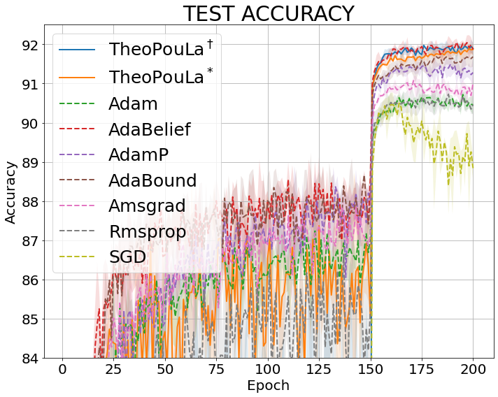
(a) VGG11 on CIFAR10

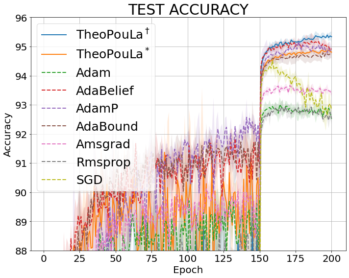
(b) ResNet34 on CIFAR10

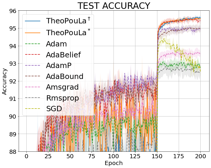
(c) DenseNet121 on CIFAR10

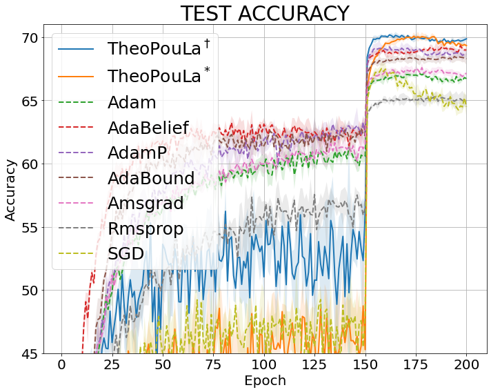
(d) VGG11 on CIFAR100

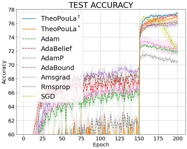
(e) ResNet34 on CIFAR100

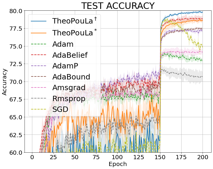
(f) DenseNet121 on CIFAR100

Figure 2: Test accuracy for VGG11, ResNet34 and DenseNet121 on CIFAR-10 and CIFAR-100. TH$\varepsilon$OPOULA^† and TH$\varepsilon$OPOULA^∗ represent the performances of TH$\varepsilon$O POULA under the best and second best hyperparameters, respectively.

E.2 Language Modeling

We conduct language modeling for Penn Treebank (PTB) data set. For this task, we train the AWD LSTM of Merity et al. [2018] for $750$ epochs. The details of models can be found in the official implementation of AWD-LSTM .

For NT-ASGD and averaged TH$\varepsilon$O POULA, the constant learning rate of $30$ is used for 2 and 3-layer LSTMs. For 1-layer LSTMs, we set to $10$. $\epsilon=100$ and $\beta=10^{10}$ are set across all the experiments.

For AdaBelief, we used the best hyperparameters reported in Zhuang et al. [2020]. Thus, we obtain the same results of AdaBelief in Zhuang et al. [2020]. Specifically, we set $\beta_{1}=0.9$, $\beta_{2}=0.999$, $\varepsilon=10^{-12}$ and an initial learning rate of $0.01$ for 2 and 3-layer LSTMs. $\lambda=0.001$ and $\varepsilon=10^{-16}$ are used for 1-layer LSTMs.

The averaging is triggered when no improvement has been made for $5$ consecutive epochs for TH$\varepsilon$O POULA. Also, AdaBelief uses a development-based learning rate decay, which decreases the learning rate by a constant factor $\delta$ if the model does not attain a new best value for $k$ epochs. We have searched the optimal hyperparameters for the development-based learning rate decay among $\delta=\{0.1,0.5\}$ and $k=\{5,10,20\}$. We have found $\delta=0.1$ and $k=5$ yield the best performance. Figure 3 displays test perplexity for different AWD-LSTM models on PTB.

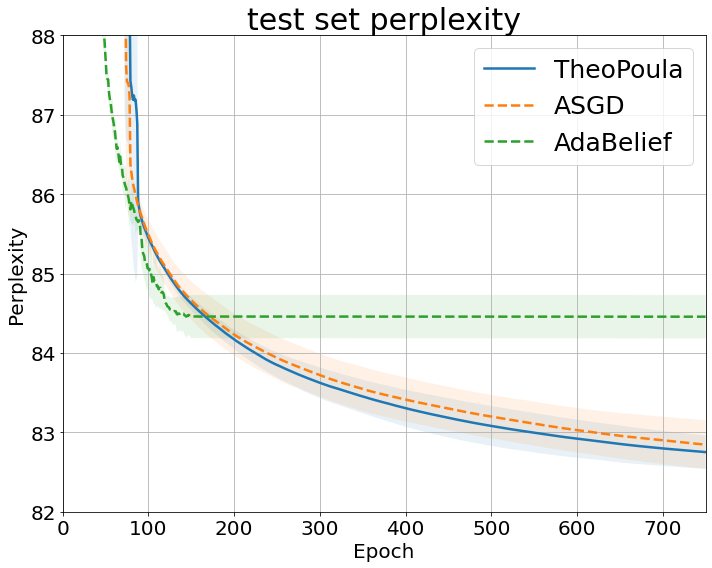
(a) 1-layer

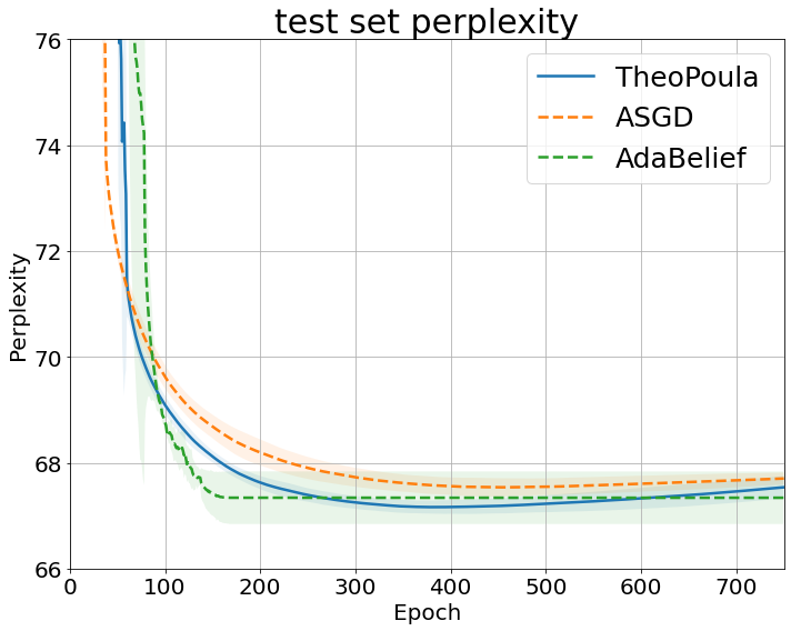
(b) 2-layer

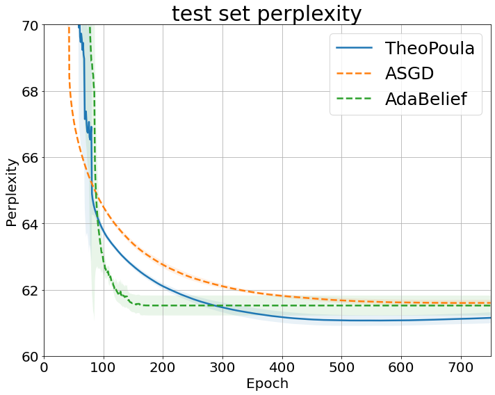
(c) 3-layer

Figure 3: Test perplexity for 1, 2 and 3-layer AWD-LSTMs on PTB

E.3 Effectiveness of the boosting function

This subsection empirically tests the effectiveness of the boosting function in our algorithm. TH$\varepsilon$O POULA without the boosting function updates the parameter as follows:

$$\theta_{0}^{\lambda}:=\theta_{0},\qquad\theta_{n+1}^{\lambda}:=\theta_{n}^{\lambda}-\lambda H_{\lambda,c}(\theta_{n}^{\lambda},X_{n+1})+\sqrt{2\lambda\beta^{-1}}\xi_{n+1},\quad n\in\mathbb{N},$$

where $H_{\lambda,c}:=(H_{\lambda,c}^{(1)}(\theta,x),\cdots,H_{\lambda,c}^{(d)}(\theta,x))^{T}$ is given by

$$H_{\lambda,c}^{(i)}(\theta,x)=\frac{G^{(i)}(\theta,x)}{1+\sqrt{\lambda}|G^{(i)}(\theta,x)|}+\eta\frac{\theta^{(i)}|\theta|^{2r}}{1+\sqrt{\lambda}|\theta|^{2r}},$$ (E.1)

and $\{\xi_{n}\}_{n\geq 1}$ is a sequence of independent standard $d$-dimensional Gaussian random variables.

Indeed, this is a special case of TH$\varepsilon$O POULA with $\epsilon=\infty$. We train VGG11, ResNet34 and DenseNet121 on CIFAR-10 and CIFAR-100 using the iterating rule of (E.1). The hyperparameters are the same with the best hyperparameters of TH$\varepsilon$O POULA. As Table 4 shows, TH$\varepsilon$O POULA without the boosting function is worsen than TH$\varepsilon$O POULA. The result indicates that the addition of the boosting function leads to a meaningful increase of test accuracy, validating that the boosting function works well for the sparsity of neural networks as expected.

Table 4: The best accuracy for VGG11, ResNet34 and DenseNet121 on CIFAR-10 and CIFAR-100. TH$\varepsilon$OPOULA^† represents the performances of TH$\varepsilon$O POULA with the best hyperparameters. TH$\varepsilon$OPOULA$(\epsilon=\infty)$ means the performance without the boosting function with the same hyperparameters.

dataset	CIFAR-10			CIFAR-100
model	VGG	ResNet	DenseNet	VGG	ResNet	DenseNet
TH$\varepsilon$OPOULA†	92.10	95.43	95.66	70.31	77.53	79.90
TH$\varepsilon$OPOULA$(\epsilon=\infty)$	91.48	94.93	95.26	68.11	75.91	77.99

Appendix F Table of Constants

Table 5 displays full expressions for constants which appear in the main results of this paper. In addition, Table 6 shows all main constants and their dependencies on key parameters such as $d$, $\beta$, the moments of $K(X_{0})$ and $\eta$.

Table 5: Explicit expression for constants with $\hat{c}$ and $\dot{c}$ from Proposition 3.14 of Chau et al. [2019].

Symbol	Full Expression
$M$	$\max\bigg{\{}M_{0},1,\frac{2\sqrt{\lambda_{\max}}d(1+\lambda_{\max}^{2})}{(2-\sqrt{\lambda}_{\max}\eta)\eta},\frac{(1+\lambda_{\max})\sqrt{d}}{\eta(2-\eta)},\frac{2^{2p-2}p(2p-1)d}{\eta\beta}\bigg{\}}$
$\widetilde{D}_{k}$	$2^{k-1}\bigg{[}(2\lambda_{\max}\sqrt{M})^{k}(\mathbb{E}[K(X_{0})](1+M^{q})+d\sqrt{\lambda}_{\max}+2\eta M^{2r+1})^{k/2}$
	$+(4d(1+\lambda_{\max}^{2})+2\eta^{2}M^{2})^{k}\bigg{]},\quad k=1,\cdots,8(2r+1)$
$A_{p}$	$\eta^{2}M^{2p}+M^{2p}\sum_{k=1}^{p}\begin{pmatrix}p\\ k\end{pmatrix}\lambda_{\max}^{k-1}\widetilde{D}_{k}$
	$+2^{2p-3}p(2p-1)\bigg{(}\frac{2dM^{2p-2}}{\beta}\sum_{k=0}^{p-1}\begin{pmatrix}p\\ k\end{pmatrix}\lambda_{\max}^{k}\widetilde{D}_{k}+\frac{2}{\beta}\bigg{(}\frac{2\lambda_{\max}}{\beta}\bigg{)}^{p-1}d^{p}(2p-1)!!\bigg{)},$
	for $p=1,\cdots,8(2r+1)$
$\overline{M}_{p}$	$\sqrt{\frac{1}{3}+4B/(3A)+4d/(3A\beta)+4(p-2)/(3A\beta)}$
$\overline{c}(p)$	$\frac{Ap}{4},\quad p=1,\cdots,8(2r+1)$
$\tilde{c}(p)$	$\frac{3}{4}Apv_{p}(\overline{M}_{p}),\quad p=1,\cdots,8(2r+1)$
$C_{1}$	$\frac{L^{2}2^{2\rho+5/2}3^{2l}}{a}(1+\mathbb{E}|X_{0}|^{2\rho})\sqrt{(1+2\mathbb{E}|\bar{\theta}^{\lambda}_{0}|^{4l}+2\frac{A_{2l}}{\eta^{2}})}$
	$\times\sqrt{8d^{2}(1+\lambda_{\max}^{4})+\eta^{4}(\mathbb{E}|\theta_{0}|^{4}+A_{2}/\eta^{2})+\frac{3}{\beta^{2}}d^{2}}$
$C_{2}$	$4\sqrt{6\mathbb{E}|K(X_{0})|^{2}(1+\mathbb{E}|\theta_{0}|^{2q}+\frac{A_{q}}{\eta^{2}})+3\lambda_{\max}d+3\eta^{2}|\bar{\theta}^{\lambda}_{\lfloor t\rfloor}|^{4r+2}}$
	$\times\sqrt{4\mathbb{E}|K(X_{0})|^{2}(1+\mathbb{E}|\theta_{0}|^{2q}+\frac{A_{q}}{\eta^{2}})+2\eta^{2}\bigg{(}\mathbb{E}|\bar{\theta}^{\lambda}_{0}|^{4r+2}+\frac{A_{2r+1}}{\eta^{2}}\bigg{)}}$
$C_{3}$	$\frac{6}{a}\bigg{[}8\mathbb{E}|K(X_{0})|^{4}(1+\mathbb{E}|\bar{\theta}^{\lambda}_{0}|^{4q}+A_{2q}/\eta^{2})+d+\eta^{2}(\mathbb{E}|\bar{\theta}^{\lambda}_{0}|^{8r+2}+A_{4r+1}/\eta^{2})\bigg{]}.$
$z_{1}$	$\frac{\hat{c}\sqrt{e^{3a}(C_{1}+C_{2}+C_{3})}}{1-\exp(-\dot{c})}\bigg{[}1+\sqrt{2\mathbb{E}|\theta_{0}|^{4}+2+2\frac{A_{2}}{\eta^{2}}}+\sqrt{2\mathbb{E}|\theta_{0}|^{4}+2+2\frac{A_{2}}{\eta^{2}}+\frac{\tilde{c}(4)}{\overline{c}(4)}}\bigg{]}$
$z_{2}$	$\frac{\sqrt{\hat{c}}e^{3a/4}(C_{1}+C_{2}+C_{3})^{1/4}}{1-\exp(-\dot{c}/2)}\bigg{(}1+\sqrt{2\mathbb{E}|\theta_{0}|^{4}+2+2\frac{A_{2}}{\eta^{2}}}+\sqrt{2\mathbb{E}|\theta_{0}|^{4}+2+2\frac{A_{2}}{\eta^{2}}+\frac{\tilde{c}(4)}{\overline{c}(4)}}\bigg{)}^{\frac{1}{2}}$
$a_{1}$	$2^{l}(\mathbb{E}[K(X_{0})]+\eta)$
$R_{0}$	$R_{0}:=\max\{\sqrt{B/A},\sqrt{2d/(\beta L\mathbb{E}(1+|X_{0}|)^{\rho})}\}$
$K$	$L\mathbb{E}[(1+|X_{0}|)^{\rho}](1+4R_{0})^{l}$
$M_{1}$	$(z_{1}+\sqrt{e^{3a}(C_{1}+C_{2}+C_{3})})$
$M_{2}$	$\hat{c}\left[1+\mathbb{E}\left[V_{2}\left(\theta_{0}\right)\right]+\int_{\mathbb{R}^{d}}V_{2}(\theta)\pi_{\beta}(d\theta)\right]$
$M_{3}$	$\sqrt{e^{3a}(C_{1}+C_{2}+C_{3})}$
$M_{4}$	$\sqrt{2\hat{c}\left(1+\mathbb{E}\left[V_{2}\left(\theta_{0}\right)\right]+\int_{\mathbb{R}^{d}}V_{2}(\theta)\pi_{\beta}(d\theta)\right)}$
$M_{5}$	$\bigg{(}\frac{a_{1}}{l+1}\sqrt{\mathbb{E}|\theta_{0}|^{2l}+\frac{A_{l}}{\eta^{2}}}+\frac{a_{1}}{l+1}\sqrt{\mathbb{E}|\theta_{\infty}|^{2l}}+2\mathbb{E}[K(X_{0})]\bigg{)}$
$M_{6}$	$\bigg{[}\frac{d}{2}\log\bigg{(}\frac{eK}{A}\bigg{(}\frac{B\beta}{d}+1\bigg{)}\bigg{)}-\log\bigg{(}1-e^{-(R_{0}\sqrt{K\beta}-\sqrt{d})^{2}}\bigg{)}\bigg{]}$

Table 6: Main constants and their dependency to key parameters

+ Constant Key parameters $d$ $\beta$ Moments of $X_{0}$ $\eta$ $A$ - - $\mathcal{O}(\mathbb{E}K(X_{0}))$ - $B$ - - $\mathcal{O}(\mathbb{E}K(X_{0})^{q+2})$ $\mathcal{O}(\frac{1}{\eta^{q+1}})$ $R$ - - $\mathcal{O}(\mathbb{E}|X_{0}|^{\rho})$ $\mathcal{O}(\frac{1}{\eta^{2r-q}})$ $a$ - - $\mathcal{O}\left(\mathbb{E}|X_{0}|^{\rho(q-1)}\right)$ $\mathcal{O}(\frac{1}{\eta^{(2r-q)(q-1)}})$ $A_{p}$ $poly(d)$ $\mathcal{O}(\frac{d}{\beta})$ $\mathcal{O}(\mathbb{E}K|X_{0}|^{p/2})$ $\mathcal{O}(\frac{1}{\eta^{p-2}})$ $\dot{c}$ $\mathcal{O}(e^{-d})$ Inherited from contraction estimates in Eberle et al. [2019] $\hat{c}$ $\mathcal{O}(e^{d})$ Inherited from contraction estimates in Eberle et al. [2019]

References

- Balles and Hennig [2018] L. Balles and P. Hennig. The sign, magnitude and variance of stochastic gradients. International Conference on Machine Learning, 2018.
- Barkhagen et al. [2021] M. Barkhagen, N. H. Chau, É. Moulines, M. Rásonyi, S. Sabanis, and Y. Zhang. On stochastic gradient Langevin dynamics with dependent data streams in the logconcave case. Bernoulli, 27(1):1–33, 2021.
- Bengio et al. [1994] Y. Bengio, P. Simard, and P. Frasconi. Learning long-term dependencies with gradient descent is difficult. IEEE transactions on neural networks, 5(2):157–166, 1994.
- Brosse et al. [2018] N. Brosse, E. Moulines, and A. Durmus. The promises and pitfalls of stochastic gradient langevin dynamics. Advances in Neural Information Processing Systems, 2018.
- Brosse et al. [2019] N. Brosse, A. Durmus, É. Moulines, and S. Sabanis. The tamed unadjusted Langevin algorithm. Stochastic Processes and their Applications, 129(10):3638–3663, 2019.
- Chau et al. [2019] H. N. Chau, É. Moulines, M. Rásonyi, S. Sabanis, and Y. Zhang. On stochastic gradient Langevin dynamics with dependent data streams: the fully non-convex case. arXiv preprint arXiv:1905.13142, 2019.
- Chen et al. [2019] X. Chen, S. Liu, R. Sun, and M. Hong. On the convergence of a class of adam-type algorithms for non-convex optimization. International Conference on Learning Representations, 2019.
- Dalalyan [2017] A. S. Dalalyan. Theoretical guarantees for approximate sampling from smooth and log-concave densities. Journal of the Royal Statistical Society: Series B (Statistical Methodology), 79(3):651–676, 2017.
- Duchi et al. [2011] J. Duchi, E. Hazan, and Y. Singer. Adaptive subgradient methods for online learning and stochastic optimization. Journal of Machine Learning Research, 12, 2011.
- Durmus and Moulines [2017] A. Durmus and É. Moulines. Nonasymptotic convergence analysis for the unadjusted Langevin algorithm. The Annals of Applied Probability, 27(3):1551–1587, 2017.
- Eberle et al. [2019] A. Eberle, A. Guillin, and R. Zimmer. Couplings and quantitative contraction rates for Langevin dynamics. Annals of Probability, pages 1982–2010, 2019.
- Erdogdu et al. [2018] M. A. Erdogdu, L. Mackey, and O. Shamir. Global non-convex optimization with discretized diffusions. Conference on Neural Information Processing Systems, 2018.
- Heo et al. [2021] B. Heo, S. Chun, S.J. Oh, D. Han S. Yun, G. Kim, Y. Uh, and J. Ha. Adamp: slowing down the slodown for momentum optimizers on scale-invariant weights. International Conference on Learning Representations, 2021.
- Huang et al. [2017] G. Huang, Z. Liu, L. Maaten, and K. Weinberger. Densely connected convolutional networks. IEEE conference on computer vision and pattern recognition, pages 4700–4708, 2017.
- Hutzenthaler et al. [2012] M. Hutzenthaler, A. Jentzen, and P. E. Kloeden. Strong convergence of an explicit numerical method for sdes with nonglobally lipschitz continuous coefficients. The Annals of Applied Probability, 22(4):1611–1641, 2012.
- Hwang [1980] C. Hwang. Laplace’s method revisited: weak convergence of probability measures. The Annals of Probability, pages 1177–1182, 1980.
- Ioffe and Szegedy [2015] S. Ioffe and C. Szegedy. Batch normalization: Accelerating deep network training by reducing internal covariate shift. International Conference on Machine Learning, pages 448–456, 2015.
- Ioffe and Szegedy [2016] S. Ioffe and C. Szegedy. Deep residual learning for image recognition. IEEE conference on computer vision and pattern recognition, pages 248–255, 2016.
- Keskar and Socher [2017] N. Keskar and R. Socher. Improving generalization performance by switching from adam and sgd. arXiv:1712.07628, 2017, 2017.
- Kingma and Ba [2015] D. Kingma and J. Ba. ADAM: A method for stochastic optimization. International Conference on Learning Representations, 2015.
- Krizhevsk [2009] A. Krizhevsk. Learning multiple layers of features from tiny images. 2009. URL http://www.cs.toronto.edu/~kriz/cifar.html.
- [22] A. Krizhevsky, V. Nair, and G. Hinton. Cifar-10 (canadian institute for advanced research). URL http://www.cs.toronto.edu/~kriz/cifar.html.
- Krylov [1985] N. V. Krylov. Extremal properties of the solutions of stochastic equations. Theory of Probability and its Applications,, 29(2):205–217, 1985.
- Krylov [1990] N. V. Krylov. A simple proof of the existence of a solution to the Itô’s equation with monotone coefficients. Theory of Probability and its Applications,, 35(3):583–587, 1990.
- Liu et al. [2020] L. Liu, H. Jiang, P. He, W. Chen, X. Liu, J. Gao, and J. Han. On the variance of the adaptive learning rate and beyond. International Conference on Learning Representations, 2020.
- Loshchilov and Hutter [2019] I. Loshchilov and F. Hutter. Decoupled weight decay regularization. International Conference on Learning Representations, 2019.
- Lovas et al. [2020] A. Lovas, I. Lytas, M. Rasonyi, and S. Sabanis. Taming neural networks with tusla: Non-convex learning via adaptive stochastic gradient langevin algorithms. arXiv preprint arXiv:2006.14514, 2020.
- Luo et al. [2019] L. Luo, Y. Xiong, Y. Liu, and X. Sun. Adaptive gradient methods with dynamic bound of learning rate. International Conference on Learning Representations, 2019.
- Marcus et al. [1999] M.P. Marcus, B. Santorini, M.A. Marcinkiewicz, and Ann Taylor. Treebank-3. 1999. URL https://doi.org/10.35111/gq1x-j780.
- Merity et al. [2018] S. Merity, N. S. Keskar, and R. Socher. Regularizing and optimizing lstm language models. International Conference on Learning Representations, 2018.
- Pascanu et al. [2013] R. Pascanu, T. Mikolov, and Y. Bengio. On the difficulty of training recurrent neural networks. Proceedings of the 30th International Conference on Machine Learning, 2013.
- Polyak and Juditsky [1992] B. Polyak and A. Juditsky. Acceleration of stochastic approximation by averaging. SIAM journal oon control and optimization, 30:835–855, 1992.
- Raginsky et al. [2017] M. Raginsky, A. Rakhlin, and M. Telgarsky. Non-convex learning via stochastic gradient Langevin dynamics: a nonasymptotic analysis. Conference on Learning Theory, 2017.
- Reddi et al. [2018] S. Reddi, S. Kale, and S. Kumar. On the convergence of ADAM and beyond. International Conference on Learning Representations, 2018.
- Roberts and Tweedie [1996] G. O. Roberts and R. Tweedie. Exponential convergence of Langevin distributions and their discrete approximations. Bernoulli, 2(4):341–363, 1996.
- Sabanis [2013] S. Sabanis. A note on tamed euler approximations. Electronic Communications in Probability, 18(47):1–10, 2013.
- Simonya and Zisserman [2015] K. Simonya and A. Zisserman. Very deep convolutional networks for large-scale image recognition. International Conference on Learning Representations, 2015.
- Tieleman and Hinton [2012] T. Tieleman and G. Hinton. Lecture 6.5-rmsprop: Divide the gradient by a running average of its recent magnitude. COURSERA: Neural Networks for Machine Learning, 2012.
- Welling and Teh [2011] M. Welling and Y. W. Teh. Bayesian learning via stochastic gradient Langevin dynamics. In Proceedings of the 28th International Conference on Machine Learning, pages 681–688, 2011.
- Wilson et al. [2017] A. C. Wilson, R. Roelofs, M. Stern, N. Srebro, and B. Recht. The marginal value of adaptive gradient methods in machine learning. Advances in Neural Information Processing Systems, 2017.
- Xu et al. [2018] P. Xu, J. Chen, D. Zou, and Q. Gu. Global convergence of Langevin dynamics based algorithms for nonconvex optimization. Conference on Neural Information Processing Systems, 2018.
- Zaheer et al. [2018] M. Zaheer, S. Reddi, D. Sachan, S. Kale, and S. Kumar. Adaptive methods for nonconvex optimization. Advances in Neural Information Processing Systems, 2018.
- Zhang et al. [2019] Y. Zhang, Ö. D. Akyildiz, T. Damoulas, and S. Sabanis. Nonasymptotic estimates for Stochastic Gradient Langevin Dynamics under local conditions in nonconvex optimization. arXiv preprint arXiv:1910.02008, 2019.
- Zhuang et al. [2020] J. Zhuang, T. Tang, Y. Ding, S. Tatikonda, N. Dvornek, X. Papademetris, and J. Duncan. Adabelief optimizer: adapting stepsizes by the belief in observed gradients. Advances in Neural Information Processing Systems, 2020.