Learning Structures for Deep Neural Networks

Abstract

In this paper, we study the automatic structure learning for deep neural networks (DNN), motivated by the observations that the performance of a deep neural network is highly sensitive to its structure and previous successes of DNN heavily depend on human experts to design the network structures. We focus on the unsupervised setting for structure learning and propose to adopt the efficient coding principle, rooted in information theory and developed in computational neuroscience, to guide the procedure of structure learning without label information. This principle suggests that a good network structure should maximize the mutual information between inputs and outputs, or equivalently maximize the entropy of outputs under mild assumptions. We further establish connections between this principle and the theory of Bayesian optimal classification, and empirically verify that larger entropy of the outputs of a deep neural network indeed corresponds to a better classification accuracy. Then as an implementation of the principle, we show that sparse coding can effectively maximize the entropy of the output signals, and accordingly design an algorithm based on global group sparse coding to automatically learn the inter-layer connection and determine the depth of a neural network. Our experiments on a public image classification dataset demonstrate that using the structure learned from scratch by our proposed algorithm, one can achieve a classification accuracy comparable to the best expert-designed structure (i.e., convolutional neural networks (CNN)). In addition, our proposed algorithm successfully discovers the local connectivity (corresponding to local receptive fields in CNN) and invariance structure (corresponding to pulling in CNN), as well as achieves a good tradeoff between marginal performance gain and network depth. All of this indicates the power of the efficient coding principle, and the effectiveness of automatic structure learning.

1 Update in 2021

This manuscript was written in January 2014 and once submitted to ICML 2014. Unfortunately, we did not continue this line of research and did not publish this article either. Today, we decide to publish it and expect the idea and empirical results can be helpful to those who would like to understand and investigate the problems such as why deep learning works.

Since 2014, several related works emerge, among which the most close ones are the information bottleneck principle (Tishby & Zaslavsky, 2015) and maximum coding rate reduction principle (Chan et al., 2021). Both of these two principles are based on supervised learning which assumes the labels of data are known, while the principle of this paper investigate the structure learning through unsupervised learning. We assume the optimal structure of neural networks can be derived from the input features even without labels. Furthermore, let $x$ , $z$, $y$ indicate the input data, the learned representation and labels respectively. Information bottleneck principle (Tishby & Zaslavsky, 2015) aims to maximize the mutual information between $z$ and $y$, meanwhile minimize the mutual information between $x$ and $z$. However, the information maximization principle in this paper aims to maximize the mutual information between $x$ and $z$. The maximum coding rate reduction principle (Chan et al., 2021), on the one hand, tries to maximize the mutual information between $x$ and $z$, which is essentially the same as information maximization principle. However, on the other hand, the $MCR^{2}$ principle also leverages the labels of data and minimize the volume of $z$ within each class. In linear model, information maximization principle leads to PCA (principal component analysis) while maximum coding rate reduction leads to LDA (linear discriminant analysis).

2 Introduction

Recent years, people have witnessed a resurgence of neural networks in the machine learning community. Indeed, systems built on deep neural network techniques (DNN) demonstrate remarkable empirical performance in a wide range of applications. For examples, convolutional neural networks keeps the records in the ImageNet challenge ILSVRC 2012 (Krizhevsky et al., 2012) and ILSVRC 2013 (Zeiler & Fergus, 2013). The core of state-of-the-art speech recognition systems are also based on DNN techniques (Mohamed et al., 2009; Deng & Yu, 2011). In the applications to natural language processing, neural networks are making steady progress too (Collobert et al., 2011; Mikolov et al., 2013).

Empirical evidences for understanding why deep neural networks works so well are also accumulated. Besides the techniques such as dropout, local normalization, and data augmentation, the evidences suggest that the architecture or structure of neural networks plays a significant role in its success. For example, an early result reported by (Jarrett et al., 2009) finds that, a two-layer architecture is always better than a single-layer one. More surprisingly, the paper observes that, given an appropriate structure, even random assignment of networks parameters can yield a decent performance. In addition, in the state-of-the-art systems such as (Krizhevsky et al., 2012; Zeiler & Fergus, 2013; Mohamed et al., 2009; Deng & Yu, 2011), the network structure, in particularly, the inter-layer connection, the number of nodes in each layer, and the depth of the networks, are all designed by human experts in a very careful and probably painful way. This requires in-depth domain knowledge (e.g., the structure of convolutional neural networks (LeCun et al., 1998) largely originates from the inspiration of biological nervous system (Hubel & Wiesel, 1962; Fukushima & Miyake, 1982), and the network structure in (Deng & Yu, 2011) heavily depend on the domain knowledge in speech recognition) or hundreds of times of trial-and-error (Jarrett et al., 2009).

Given this situation, a natural question arises: can we learn a good network structure for DNN from scratch in a fully automatic fashion? What is the principled way to achieve this? To the best of our knowledge, the studies on these important questions are still very limited. Only (Chen et al., 2013) shows the possibility of learning the number of nodes in each layer with a nonparametric Bayesian approach. However, there is still no attempt on the automatic learning of inter-layer connections and the depth of DNN. These are exactly the focus of our paper.

For this purpose, we borrow an important principle, called the efficient coding principle, from the domain of biological nervous systems, in which area there exists tremendous research work on understanding the structure of human brains. The principle basically says that a good structure (brain structure in their case and the structure of DNN in our case) forms an efficient internal representation of external environments (Barlow, 1961; Linsker, 1988). Rephrased by our familiar language, the principle suggests that the structure of a good network should match the statistical structure of input signals. In particular, it should maximize the mutual information between the inputs and outputs, or equivalently maximize the entropy of the output signals under mild assumptions. While the principle seems intuitive and a little informal, we show that it has a solid theoretical foundation in terms of Bayesian optimal classification, and thus has a strong connection with the optimality of the neural networks from the machine learning perspective. In particular, we first show that the principle suggests us to maximize the independence between the output signals. Then we notice that the top layer of any neural network is a softmax linear classifier, and the independency between the nodes in the top hidden layer is a sufficient condition for the softmax linear classifier to be the Bayesian optimal classifier. This theoretical foundation also provides us a clear way to determine the depth of the deep neural networks: if after multiple layers of non-linear transformations (learned under the guidelines of the efficient coding principle) the hidden nodes become statistically independent of each other, then there is no need to add another hidden layer (i.e., the depth of the network is finalized) since we have already been optimal in terms of the classification error.

We then investigate how to design structure learning algorithm based on the principle of efficient coding. We show that sparse coding can implement the principle under the assumption of zero-peaked and heavy-tailed prior distributions. Based on this discovery, we design an effective structure learning algorithm based on global group sparse coding. When customized for image analysis, we discuss how the proposed algorithm can learn inter-layer connections, handle invariance, and determine the depth.

We conduct a set of experiments on a widely used dataset for image classification. We have several interesting findings. First, although we have not imposed any prior knowledge onto the structure learning process, the DNN with our automatically learned structure can provide a very competitive classification accuracy, which is very close to the well-tuned CNN model that is designed by human experts. Second, our algorithm can automatically discover the local connection structure, simply due to the match of the statistical structure of input signals. Third, we notice that the pooling operation specifically designed in CNN can also be automatically implemented by our learning algorithm based on group sparse coding. All these results demonstrate the power of automatic structure learning based on the efficient coding principle.

While our work is just a preliminary step towards automatic structure learning, we have seen very positive signs suggesting that structure learning could be an important direction to better understand DNN, to further improve the performance of DNN, and to generalize the application scope of DNN based learning algorithms.

3 The Principle for Structure Learning

The key of unsupervised structure learning for DNN is to adopt an appropriate principle to guide the procedure of structure learning. In this section, we describe our used principle and discuss its advantages for structure learning.

Figure 1: Fig. (a) shows an pipeline of linear and nonlinear transformation; Fig. (b) shows an example of the cumulated distribution function (CDF) transformation, which can map arbitrary distribution into a uniform distribution in $[0,1]$.

To guide the structure learning for deep neural networks, we borrow a principle from computational neuroscience. In fact, various hypotheses have been proposed to understand the magic structure of biological nervous system in the literature. The core problem under investigation include: what is the goal of sensory coding or what type of neuronal representation is optimal in an ecological sense? Of all the attempts on answering this question, the principles rooted in information theory have been proved to be successful.

For ease of illustration of these principles, we give some notations first. Figure 1 shows how the data go through one layer of a typical neural network. The input $\mathbf{X}$ is firstly processed by a linear transformation $\mathbf{W}$ and followed by a component-wise transformation $\mathbf{\sigma}$, in which each component is usually a bounded, invertible nonlinear function. That is,

$$Z_{i}=\sigma_{i}(U_{i})=\sigma_{i}(\mathbf{W}_{i}^{T}{\mathbf{X}})$$ (1)

Without loss of generality, the range of $\sigma_{i}$ is usually assumed $[0,1]$. $\mathbf{Z}$ is the neuronal representation or a coding of the input $\mathbf{X}$.

Among the information-theoretic principles proposed in the literature, the redundancy reduction principle developed by Barlow (Barlow, 1961) has been at the origin of many theoretical and experimental studies. Let $I(\mathbf{Z})$ denote the mutual information between output units. Barlow’s theory proposes that, the output of each unit should be statistically independent from each other in an optimal neural coding. That is, the objective function is the minimization of $I(\mathbf{Z})$. Another principle developed by Linsker (Linsker, 1988) advocates that the system should maximize the amount of information that the output conveys about the input signal, that is, maximizing $I(\mathbf{X};\mathbf{Z})$. As shown in the following theorem, the aforementioned principles are actually equivalent to each other under certain conditions.

Theorem 1.

Let the component-wise nonlinear transfer function $\mathbf{\sigma}_{i}$ be the cumulated distribution function (CDF) of $U_{i}$, minimizing $I(\mathbf{Z})$ is equivalent to maximizing $I(\mathbf{X};\mathbf{Z})$.

A sketch proof is given in supplementary material. The theory indicates that for bounded output neural networks, minimizing the mutual information between outputs is equivalent to maximizing the mutual information between inputs and outputs. Due to this equivalence, we will not distinguish the two principles, and will uniformly refer to them as “efficient coding principles”.

Since the efficient coding principle is rooted in computational neuroscience and information theory, one may wonder whether it really ensures optimal neural network structures from the machine learning perspective. Through the following theorem we show that this principle has a strong theoretical connection with pattern classification tasks.

Theorem 2.

(Minsky, 1961) With (conditional) independent features, linear classifier is optimal in the sense of minimum Bayesian error.

Actually, this theorems has its particular implication in the context of structure learning for deep neural networks. As we know, no matter how a deep neural network is structured, its top layer is always a softmax linear classifier. Then according to the above theorem, if we can achieve the independency between the nodes in the top hidden layer by means of structure learning, then it will ensure (as a sufficient condition) that the softmax linear classifier would be the Bayesian optimal classifier. In other words, there is no need to adopt more complicated non-linear classifiers at all. In this sense, this theoretical foundation also provides us a clear way to determine the depth of the deep neural networks: if after multiple layers of non-linear transformations (learned under the guidelines of the efficient coding principle) the hidden nodes become statistically independent of each other, then we should stop growing the depth of the neural networks since we have already been optimal in terms of the possibly best classification error we could ever get.

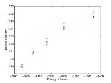
Figure 2: The correlation between feature entropy and classification accuracy.

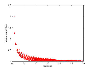
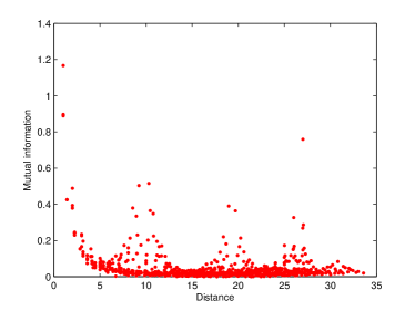
Figure 3: Fig. (a) The mutual information between pixels decays with the increasing of the spatial distance between pixels; Fig. (b) The similar decay behavior can be observed when each location is represented as an edge direction. This figure demonstrates that, with pixel representation, two locations seems independent if the spatial distance exceeds 10. However, after extracting edge directions at each location and represent the location with the edge direction, two locations are no longer seemingly independent. Such observation implies the redundancies emerge with more abstract representation.

4 Empirical Observations

In this section, we show some empirical studies regarding the efficient coding principle. For this purpose, we need to compute the coding efficiency (or information gain) provided by a layer of neural network (in terms of the change of the mutual information). Please refer to the Appendix for the method we used.

4.1 Coding Efficiency and Classification Accuracy

We generate a set of random structures and use them to extract features from whitened CIFAR-10 data set. The coding efficiency of the extracted features and the corresponding classification on training set are evaluated . Figure 2 demonstrates the relation between feature entropy and classification accuracy of softmax classifier. A positive correlation between entropy and classification accuracy can be observed. Noting that the efficient coding principle is an unsupervised objective function, this positive correlation is somewhat surprising.

4.2 Spatial Redundancy of Images

Figure 3 shows the redundancy properties of natural images. The result is obtained at whitened CIFAR-10 data. The large value of mutual information between nearby elements indicates the redundancy of information. In both figures, we can observe the decay behavior of mutual information with the increasing of spatial distance. This suggests the elements sufficiently far-away from each other are nearly independent. This is not surprising, as the phenomenon is already widely formulated by Markov assumption in various probabilistic model. Interestingly, Figure 3 which shows that, after feature extraction by edge detector, the redundancies between nearby pixels are removed, however, new dependencies among edges emerge. The dependencies between edges spread much broader than that of pixels. This suggests that a single layer transformation is not sufficient for the purpose of redundancy reduction. We need another transformation to remove the redundancies between edge representations.

4.3 Multi-layer Redundancy Reduction

Figure 4 illustrates entropy increasing after adding more layers of transformation. We train several layers of Gaussian-binary RBM on contrast normalized CIFAR-10 and several layers of sparse coding on whitened CIFAR-10 . We can observe: (1), For both RBM and sparse coding, an additional layer bring further entropy gain though the marginal gain vanishes with the number of layers. (2), the sparse coding produce features with much higher entropy than RBM because of sparse coding is more dedicated to the goal of redundancy reduction.

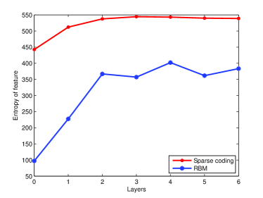
Figure 4: With RBM and sparse coding, adding more layer always help remove redundancy further. However, the gain of redundancy reduction gradually becomes marginal.

5 Algorithms

In this section, we propose algorithms for structure learning based on the principle of efficient coding.

5.1 Implementing the Principle by Sparse Coding

The transformation in Figure 1 shows how to get $\mathbf{U}$ from $\mathbf{X}$ through $\mathbf{U}=\mathbf{W}^{T}\mathbf{X}$. Inversely, $\mathbf{X}$ can be viewed as being generated by a probabilistic process governed by $\mathbf{U}$, such as

$$\mathbf{X}=\mathbf{D}^{T}\mathbf{U}+\mathbf{N}$$ (2)

where $\mathbf{N}$ is a vector of independently and identically distributed Gaussian noise, $\mathbf{D}$ describes how each source signal generates an observation vector. If the dimensions of $\mathbf{X}$ and $\mathbf{U}$ are equal and transformation matrix $\mathbf{W}$ is full rank, a trivial relation between $\mathbf{V}$ and $\mathbf{W}$ is $\mathbf{W}^{T}\mathbf{D}=\mathbf{I}$, where $\mathbf{I}$ is an identify matrix. In this way, learning optimal data transformation matrix $\mathbf{W}$ is equivalent to inferring the optimal data generating matrix $\mathbf{D}$.

Usually, to infer the simplest possible signal formation process, some additional assumptions on the prior distribution of $\mathbf{U}$ are made. As the efficient coding principle indicates, the independent or factorial codes are preferred, that is, assuming

$$p(\mathbf{U})=\prod_{i}p(U_{i}).$$ (3)

When $p(U_{i})$ is a distribution peaked at zero with heavy tails, it can be shown the model leads to the so-called sparse coding (Field, 1994). Therefore our structure learning algorithm described in the next subsection is based on sparse coding.

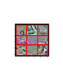
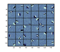
Figure 5: (a) An example of synthesize images: each image is composed of 9 blocks, and each block is sampled from a random patch of a random image. (b) 36 basis learned on the synthesized image set by sparse coding. Apparently, each basis only focuses on one block of the input image.

We construct a synthesized data set from whitened CIFAR-10. Each image consists of $3\times 3$ blocks, each of which is sampled from a random location of a random image. We can assume the pixels from different blocks are independent from each other, while the pixels in the same block possess the statistical properties of natural images. An ideal algorithm should discover and converge to the correct structure. That is, each basis is only connected to pixels in a single block. We evaluated RBM, sparse auto-encoder, and sparse coding. Sparse coding (see Fig. 5) is the only one that can perfectly recover the block structures.

5.2 The Proposed Algorithms

Algorithm 1 shows how to learn the structure from unsupervised data. As shown in the algorithm, we learn the structure layer by layer in a bottom-up manner. We put the raw features at layer $1$ and learn the connection between layer $1$ and layer $2$ given the predefined number of nodes in layer $2$. Specifically, the inter-layer connection is initialized with full connections. Trained on unlabeled data, due to the ICA properties of sparse coding, the inter-layer connection will converge to a sparse connected network. In other words, the weights of most of the edges will converge to zero during the learning process. After the connection between layer $k$ and $k+1$ has been learnt, we can estimate the entropy of layer $k+1$ according to Equation 16 and compare it with that of layer $k$. If the entropy gain between the two layers is smaller than a threshold $\epsilon$, we terminate the learning process; otherwise we add layer $k+2$ and continue to learning process. In other words, the depth of the network is determined according to the cues of entropy gain.

Algorithm 2 shows how to learn a better DNN based on the structure output by Algorithm 1 and supervised data. First, the learned sparse connection and the weights are used to initialize a multi-layer feed-forward network. The inter-layer connection inherits from the structure mask learned in Algorithm 1, and the weights of connection is initialized by the weights learned by sparse coding. Then via training on labeled data, the weights are fine-tuned further.

While the two algorithms look quite similar to several existing algorithms at the first glance, we would like to highlight and elaborate several differences and some implementation details as follows.

Algorithm 1 Structure Learning with Sparse Coding

1:  Input: $\mathbf{X}$, each column is an example $\mathbf{X}_{i}\in\mathcal{R}^{d}$

2:  Output: dictionary $\mathbf{D}_{k}$, structure mask $\mathbf{M}_{k}$, depth $K$

3:  Initialize $k=0$, $\mathbf{U}_{k}=\mathbf{X}$

4:  repeat

5:     Whiten $\mathbf{U}_{k}$

6:     $\mathbf{D}_{k},\!\mathbf{U}_{k+1}\!\!=\!\!\underset{\mathbf{D}_{k},\mathbf{U}_{k+1}}{\operatorname*{arg\,min}}\|\mathbf{U}_{k}-\mathbf{D}_{k}^{T}\mathbf{U}_{k+1}\|_{2}\!+\!\lambda\|\mathbf{U}_{k+1}\|_{1}$

7:     Calculate $\mathbf{M}_{k}$ by thresholding $\mathbf{D}_{k}$

8:     $\mathbf{Z}_{k+1}=\sigma(\mathbf{U}_{k+1})$, where $\sigma$ is feature-wise CDF

9:     Estimate $H(\mathbf{Z}_{k+1})$

10:     $k=k+1$

11:  until $|\frac{H(\mathbf{Z}_{k+1})-H(\mathbf{Z}_{k})}{H(\mathbf{Z}_{k})}|<\epsilon$

12:  $K=k+1$

Algorithm 2 Back-propagation with Structure Priming

1:  Input: $\mathbf{X}$, $\mathbf{D}_{k}$, $\mathbf{M}_{k}$, $k=1,\ldots,K$

2:  Output: $\mathbf{W}_{k}$, $k=1,\ldots,K$

3:  $\mathbf{U}_{0}=\mathbf{X}$

4:  $\mathbf{W}_{k}=\mathbf{M}_{k}\circ\mathbf{D}_{k}$ for $k=1,\cdots,K$

5:  /* Forward pass */

6:  for $k=0$ to $K$ do

7:     $\mathbf{U}_{k+1}=\mathbf{W}_{k}^{T}\mathbf{U}_{k}$

8:     $[\mathbf{U}_{k+1}]_{i}=\mathrm{sign}([\mathbf{U}_{k+1}]_{i})(|[\mathbf{U}_{k+1}]_{i}|-\lambda)_{+}$

9:  end for

10:  /* Back-propagation */

11:  $\delta\mathbf{U}_{K}=\frac{\partial\mathrm{Loss}}{\partial\mathbf{U}_{K}}$

12:  for $k=K$ down to $1$ do

13:     $[\delta\mathbf{U}_{k}]_{i}=0$ if $[\mathbf{U}_{k}]_{i}=0$

14:     $\delta\mathbf{U}_{k-1}=\mathbf{W}_{k-1}\mathbf{U}_{k}$

15:     $\delta\mathbf{W}_{k-1}=\mathbf{U}_{k-1}\delta\mathbf{U}_{k}^{T}$

16:     $\delta\mathbf{W}_{k-1}=\mathbf{M}_{k-1}\circ\delta\mathbf{W}_{k-1}$

17:     $\mathbf{W}_{k-1}=\mathbf{W}_{k-1}-\gamma\delta\mathbf{W}_{k-1}$

18:  end for

Training sparse coding in global range

The dramatic difference between the usage of sparse coding in this paper and that of existing work is that, the sparse coding is trained in global range. Take image as an example, here we train sparse coding on the whole image instead of traditional way which trains sparse coding on small patches (Yang et al., 2009). Therefore, we do not need to predefine the inter-layer connection such as the spatial range of local connection in convolutional networks. Instead, the algorithm itself is able to learn the optimal inter-layer connections. We will see in Section 6, the inter-layer connections learned on images happens to resemble the local connection structure in CNN. We notice that deconvolutional network proposed in (Zeiler et al., 2010) also trains sparse coding on whole image; however, like the patch-based sparse coding, it also needs a pre-determined spatial range for convolutional filter.

Sparsifying inter-layer connection

Once obtaining $\mathbf{D}_{k}$ by Algorithm 1, we know the strength of each connection between adjacent-layer neurons. Intuitively, the weak connection can be removed without significantly affect the behavior of network. Concretely, a binary mask matrix $\mathbf{M}_{k}$ is calculated by thresholding $\mathbf{D}_{k}$

$$[\mathbf{M}_{k}]_{i}=\left\{\begin{array}[]{rl}1,&|[\mathbf{D}_{k}]_{i}|\geq t\\ 0,&\mathrm{otherwise}\end{array}\right.$$ (4)

The parameter $t$ can be chosen according to what density of the mask matrix $\mathbf{M}_{k}$ we expect. For example, if we want to keep $10\%$ connections in the network, we can calculate the histogram of the absolute value in $\mathbf{D}_{k}$ and choose $t$ at the position of $10\%$ quantile. The resulting $\mathbf{M}_{k}$ will act as a structure priming for the feed-forward network in Algorithm 2.

Handling invariance

In tasks such as image classification, invariance based on pooling is crucial for practical performance. The output of neurons who have similar receptive fields are aggregated through an OR operation to obtain shift invariance. To endow the algorithm with this capability, the neurons should firstly be separated into overlapping or non-overlapping groups according to their selectivities. Since Algorithm 1 is based the sparse coding framework, it can be easily modified to handle invariance using group lasso (Yuan & Lin, 2006). With group lasso, the dictionary learning becomes

$$\mathbf{D}_{k}=\underset{\mathbf{D}_{k}}{\operatorname*{arg\,min}}\|\mathbf{U}_{k}\!-\!\mathbf{D}_{k}^{T}\mathbf{A}\|_{2}\!+\!\lambda\sum_{n}\!\sum_{g}\|\mathbf{A}_{g}^{n}\|_{2}$$ (5)

where $\mathbf{A}_{g}^{n}$ denotes the reconstruction coefficients of the $n$-th example in the $g$-th group. Also, the shrinkage operation in FISTA (Beck & Teboulle, 2009) algorithm will change accordingly.

Back-propagation with structure priming

Both $\mathbf{M}_{k}$ and $\mathbf{D}_{k}$ provide structure priming for feed-forward network. The weights $\mathbf{W}_{k}$ are initialized as $\mathbf{M}_{k}\circ\mathbf{D}_{k}$ in feed-forward pass, and $\mathbf{M}_{k}$ also mask the gradient $\delta\mathbf{W}_{k-1}$ in back-propagation by

$$\delta\mathbf{W}_{k-1}=\mathbf{M}_{k-1}\circ\mathbf{W}_{k-1}$$ (6)

where $\circ$ denotes Hadamard product. This implementation is the same as DropConnect approach in (Wan et al., 2013). However, in DropConnect, the mask matrix is randomly generated and also it only used in full connection layer.

One step ISTA approximation

Besides using the dictionary $\mathbf{D}_{k}$ to initialize $\mathbf{W}_{k}$, we also would like the feature map to inherit the sparse properties from sparse coding. Therefore, we implement the feed-forward transformation as a one-step ISTA approximation to the solution of lasso. The idea comes from (Gregor & LeCun, 2010) which uses several steps to obtain an efficient approximation to lasso. The shrinkage operation for standard sparse coding and group sparse coding are

$$[\mathbf{U}_{k+1}]_{i} = \mathrm{sign}([\mathbf{U}_{k+1}]_{i})(|[\mathbf{U}_{k+1}]_{i}|-\lambda)_{+}$$ (7)

$${}[\mathbf{U}_{k+1}]_{i} = \mathrm{sign}([\mathbf{U}_{k+1}]_{i})(1-\frac{\lambda}{\|[\mathbf{U}_{k+1}]_{g}^{i}\|_{2}})_{+}$$ (8)

where $\|[\mathbf{U}_{k+1}]_{g}^{i}\|_{2}$ indicates the $\ell$-2 norm of the group variables $[\mathbf{U}_{k+1}]_{i}$ belongs to. Note that the nonlinear transfer function used in feed-forward network is different from the transfer function used for estimating entropy $H(\mathbf{Z}_{k})$ where the transfer function the CDF of feature map.

CUDA implementation of sparse coding

Training a sparse coding model on whole images instead of patches is much demanding to computation resource. In our experiments, even the highly optimized sparse modeling package SPAMS (Mairal, 2010) requires several days to convergence. Regarding that GPGPU has been a common option for deep learning algorithm, we implement a CUDA sparse coding based on FISTA algorithm. As noted in (Gregor & LeCun, 2010), coordinate descent (CD) may be the fastest algorithm for sparse inference, it is true for CPU implementation. However, CD algorithm is not innate to parallel implementation due to its sequential nature. Our CUDA implementation of an online sparse coding algorithm based on FISTA algorithm speedup the process $7\!\sim\!10$ times over SPAMS.

6 Experiments

Table 1: Classification accuracies of baseline convolutional neural network.

ID	Configuration	Test accuracy
cudaconv	Adaptive LR	$81.0\%$
standard	Fixed LR	$77.5\%$
nodropout	- dropout	$75.7\%$
nopadding	- padding	$73.3\%$
nonorm	- normalization	$73.1\%$
nopooling	- pooling	$65.4\%$
2conv	nonorm with 2 conv	$72.5\%$
1conv	nonorm with 1 conv	$60.4\%$

6.1 Baseline and experimental protocols

All the experiments are carried out on the well-known CIFAR-10 data set. It contain 10 classes and totally has 50000 and 10000 $32\times 32$ color images in training and testing set respectively. As a baseline, we reproduce the cuda-convnet experiments on CIFAR-10 (Krizhevsky et al., 2012). In our implementation, we don’t use the data augmentation technique such as image translation and horizontal reflection, except that the mean image is subtracted from all the images as the cuda-convnet setting does. With an adaptive learning rate, we get an $81\%$ test accuracy with a single model. Since we are focusing on the network structure such as inter-layer connection and depth, we evaluate the contribution of techniques such as adaptive learning rate, dropout, padding and local normalization to the baseline system. These results are reported in Table 1. Note that in the table, the configuration in each line is modified from the above line without otherwise stated. Therefore, the NONORM is a setting without modules such as adaptive learning rate, dropout, padding and local normalization. This setting reflects the contribution of network architecture. If we further remove the pooling layer from NONORM, the performance drops to $65.4\%$, which implies pooling plays a significant role in this task. Removing the $3$-rd convolutional layer from NONORM, the performance drops slightly to $72.5\%$, which implies the $3$-rd convolution layer contributes marginally. If further removing the $2$-nd convolutional layer from 2CONV, the accuracy drops dramatically to $60.4\%$, which indicates two convolutional layers are essential.

Different from the input of convolutional network, the input images to sparse coding are all whitened. Empirically, we find whitening is crucial for sparse coding to get meaningful structure . In both CNN and our algorithm, the learning rate is fixed to $0.001$. Without otherwise stated, the network includes a 10-output softmax layer. The sparse coding dictionaries in all the layers are with 2048 dimension and group size is 4. All the experiments are carried out on a Tesla T20K GPU.

6.2 Overall performance

Table 2: Classification accuracies of structure learning.

ID	Configuration	Test accuracy
1layer	512	$63.0\%$
2layer	512/512	$68.0\%$
3layer	512/512/512	$69.8\%$

From Table 2, we can observe that the single layer network of learned structure achieves a test accuracy $63.0\%$ which outperforms $60.4\%$ of the single layer setting in Table 1. The two layer architecture achieves a performance $68\%$ which outperforms one layer model but is inferior to $72.5\%$ produced by CNN with two convolutional layer.

6.3 Evaluating inter-layer connection density

Table 3: Evaluating the role of inter-layer connections.

Density	random	RBM	sparse coding
$0.1\%$	$30.2\%$	$23.2\%$	$40.7\%$
$0.25\%$	$31.6\%$	$28.4\%$	$40.1\%$
$0.5\%$	$30.3\%$	$31.3\%$	$51.2\%$
$10\%$	$48.2\%$	$39.7\%$	$57.2\%$
$30\%$	$54.7\%$	$39.6\%$	$56.2\%$
$70\%$	$56.2\%$	$39.4\%$	$56.6\%$

To demonstrate the role of inter-layer connection, we compare three types of structures in a single layer network: (1) randomly generated structures, (2) structures by sparsifying restricted Boltzmann machines (RBM), (3) structures learned by sparse coding. We define the connection density as the ratio between active connections in structure mask $\mathbf{M}_{k}$ and the number of full connections. As shown in Table 3 we evaluate the three settings in several connection density level. Basically, we can observe denser connections bring performance gain. However, the performance saturates even keeping randomly $30\%$ connections. The structures generated by sparse coding outperform the random structure. Surprisingly, structures generated by RBM are even inferior to random structures. In the learned structure, at the same density level, sparse coding always outperforms RBM. For sparse coding, by keep $10\%$ connections is sufficient. Theoretically, a full connection network can emulate any sparse connection ones just by setting the dis-connected weights of the to zeros. If a sparsely connected network is known to be optimal, ideally, a full connection network with appropriate weights can yield exactly the same behavior. However, the BP algorithm usually can not converge to this optimal weights, due to the local optimum properties.

6.4 Evaluating the role of structure mask

Table 4: Evaluating the role of structure mask.

Setting	One layer	Two layer
BP	$57.9\%$	$50.2\%$
Weight	$57.6\%$	$57.4\%$
Weight+BP	$63.7\%$	$62.4\%$
Mask+BP	$58.8\%$	$58.1\%$
Weight+Mask+BP	$64.0\%$	$68.6\%$

To investigate the role of the learned structure mask, we carry out the following experiments: (1) randomly initialized BP; (2), initializing the network parameter without fine-tuning; (3), initializing the network parameter with pre-trained dictionary and fine-tuned with BP; (4), restricting the network structure with learned mask and randomly initializing the parameters, finally fine-tuning with BP; (5), restricting the network structure with mask and initializing the connection parameters with pre-trained dictionary, finally fine-tuning with BP. The results are reported in Table 4. We can observe that, even use the pre-trained dictionary as a feature extractor, it significantly outperforms BP with random initialization. Fine-tuning with BP always brings performance gain. The Mask+BP outperforming BP indicates that the structure prior provided by sparse coding is very useful. Finally, the strategy of combining Weight+Mask+BP outperforms all the others.

6.5 Evaluating network depth

Table 2 shows the performances of networks with different depth. We can observe that adding more layers is helpful, however the marginal performance gain diminishes as the depth increases. Interestingly, Figure 2 shows a similar behavior of coding efficiency. This empirically justifies the approach determining the depth by coding efficiency.

7 Conclusions

In this work, we have studied the problem of structure learning for DNN. We have proposed to use the principle of efficient coding principle for unsupervised structure learning and have designed effective structure learning algorithms based on global sparse coding, which can achieve the performance as good as the best human-designed structure (i.e., convolutional neural networks).

For the future work, we will investigate the following aspects. First, we have empirically shown that redundancy reduction is positively correlated to accuracy improvement. We will explore the theoretical connections between the principle of redundancy reduction and the performance of DNN. Second, we will extend and apply the proposed algorithms to other applications including speech recognition and natural language processing. Third, we will study the structure learning problem in the supervised setting.

8 Appendix

Theorem 3.

Let the component-wise nonlinear transfer function $\mathbf{\sigma}_{i}$ be the cumulated distribution function (CDF) of $U_{i}$, minimizing $I(\mathbf{Z})$ is equivalent to maximizing $I(\mathbf{X};\mathbf{Z})$.

9 The Proof Sketch of Theorem 3

Under the conditions of no noise (Bell & Sejnowski, 1995) or only additive output noise (Nadal & Parga, 1994), the term $H(\mathbf{Z}|\mathbf{X})$ has no relation to the transformation $\mathbf{W}$ and $\mathbf{\sigma}$. Therefore, we have

Lemma 1.

(Nadal & Parga, 1994) Maximizing the mutual information $I(\mathbf{X};\mathbf{Z})$ between input and output is equivalent to maximizing the output entropy $H(\mathbf{Z})$ under no noise or only additive output noise.

Furthermore, as shown in Figure 1, when adopting each bounded and invertible transfer function $\sigma_{i}$ as the cumulated distribution function (CDF) of the linear output $U_{i}$, each $Z_{i}$ follows a uniform distribution in $[0,1]$ and thus $H(Z_{i})$ achieves its maximum value. In this way, we have

Lemma 2.

(Yand & Amari, 1997) Maximizing $H(\mathbf{Z})$ is equivalent to minimizing $I(\mathbf{Z})$ when the component transfer function $\sigma_{i}$ is the CDF of $U_{i}$.

Now we can prove Theorem 3, which states the equivalence between the maximum information preservation principle of (Linsker, 1988) and the the redundancy reduction principle of (Barlow, 1961).

Proof.

Firstly, we have the following basic facts,

$$I(\mathbf{X};\mathbf{Z}) = H(\mathbf{Z})-H(\mathbf{Z}|\mathbf{X})$$ (9)

$$H(\mathbf{Z}) = \sum_{i}H(Z_{i})-I(\mathbf{Z})$$ (10)

Using the conclusion of Lemma 1 and Lemma 2, we know that maximizing $I(\mathbf{X};\mathbf{Z})$ is equivalent to minimizing $I(\mathbf{Z})$ under the given conditions. ∎

10 How to Measure the Efficiency Gain

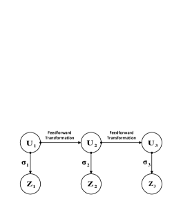
Figure 6: Measuring high-dimensional mutual information via CDF transfer function

To determine the depth of a feed-forward neural networks, we need to know at what depth the additional layer will not bring efficiency gain. Remember that the efficiency means fewer redundancies among all dimensions, therefore, we need to measure the independence between all all features in the same layer. As shown in Figure 6, let $\mathbf{U}_{i},i=1,2,3$ be three feature maps in a feed-forward networks, direct computing $I(\mathbf{U}_{1})$, $I(\mathbf{U}_{2})$ and $I(\mathbf{U}_{3})$ are infeasible for high dimensional data. This paper develops a technique to quantitatively measure those criteria. (For simplicity of analysis, we assume the dimensions of all the layer are the same).

Lemma 3.

If $\sigma_{i}$ is the CDF of $U_{i}$, $I(\mathbf{U})=-H(\mathbf{Z})$ holds.

Proof.

Since the CDF transfer function will make each output $Z_{i}$ with a uniform distribution in $[0,1]$, $H(Z_{i})$ will be zero. Therefore, $I(\mathbf{Z})=-H(\mathbf{Z})$. The lemma 4 states that $I(\mathbf{U})=I(\mathbf{Z})$ if $\sigma_{i}$ is continuous and invertible. Apparently, the CDF transfer function satisfies this condition. Thus, $I(\mathbf{U})=-H(\mathbf{Z})$. ∎

Lemma 4.

If the component-wise transfer function $\sigma_{i}$ in $Z_{i}=\sigma_{i}(U_{i})$ is continuous and invertible, $I(\mathbf{U})$ equals $I(\mathbf{Z})$.

Proof.

Firstly, we know the facts

$$I(\mathbf{Z}) = \sum_{i}H(Z_{i})-H(\mathbf{Z})$$ (11)

$$I(\mathbf{U}) = \sum_{i}H(U_{i})-H(\mathbf{U})$$ (12)

$$H(Z_{i}) = H(U_{i})+\int_{U_{i}}\mathrm{d}U_{i}p(U_{i})\log|\frac{\partial Z_{i}}{\partial U_{i}}|$$ (13)

$$H(\mathbf{Z}) = H(\mathbf{U})+\int_{\mathbf{U}}\mathrm{d}\mathbf{U}p(\mathbf{U})\log|J|$$ (14)

where $|\cdot|$ denotes the absolute value and $J$ indicates the determinant of Jacobian matrix, that is, $J=\mathrm{det}([\frac{\partial Z_{i}}{\partial U_{j}}]_{ij})$. Note that the continuous and invertible $\sigma_{i}$ guarantees that $\log|\frac{\partial Z_{i}}{\partial U_{i}}|$ and $\log|J|$ are well-defined. To prove $I(\mathbf{Z})=I(\mathbf{U})$, we must prove

$$\int_{\mathbf{U}}\mathrm{d}\mathbf{U}p(\mathbf{U})\log|J|=\sum_{i}\int_{U_{i}}\mathrm{d}U_{i}p(U_{i})\log|\frac{\partial Z_{i}}{\partial U_{i}}|$$ (15)

It is straightforward since $\sigma_{i}$ is component-wise transfer function, the Jacobian matrix is a diagonal matrix. ∎

11 Nonparametric Entropy Estimation

Estimating the entropy of high dimensional continuous random vectors such as $H(\mathbf{Z})$ is an challenging problem in both theories and applications. For a comprehensive review, please refer to (Beirlant et al., 1997). Here, we use a nonparametric entropy estimator based on $k$-nearest neighbor distances, since empirically it demonstrates better convergence properties (Kraskov et al., 2004)

$$\hat{H}(\mathbf{Z})=-\psi(k)+\psi(N)+\log c_{d}+\frac{d}{N}\sum_{i=1}^{N}\log\epsilon(i)$$ (16)

in which $d$ is the dimension of random vector, $N$ denotes the size of sample, $\psi(\cdot)$ is a digamma function, $c_{d}$ equals $\pi^{\frac{d}{2}}/{\Gamma(1+\frac{d}{2})}/2^{d}$, $\epsilon(i)$ denotes twice the distance from the $i$-th example to its $k$-th neighbor. $k$-d tree can be used to serve efficient nearest neighbor queries.

12 Visualization

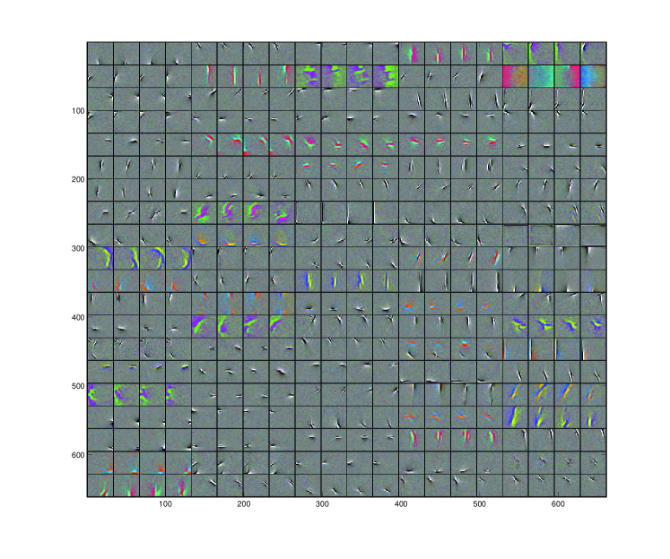
Figure 7: A sample of the learned basis by group sparse coding.

References

- Barlow (1961) Barlow, H. Possible principles underlying the transformation of sensory messages. In Rosenblith, W. (ed.), Sensory Communication. MIT Press, Cambridge, 1961.
- Beck & Teboulle (2009) Beck, A. and Teboulle, M. A fast iterative shrinkage-thresholding algorithm for linear inverse problems. SIAM J. Img. Sci., 2(1):183–202, 2009.
- Beirlant et al. (1997) Beirlant, J., Dudewicz, E. J., Györfi, L., and Van Der Meulen, E. C. Nonparametric entropy estimation: An overview. International Journal of Mathematical and Statistical Sciences, 6(1):17–39, 1997.
- Bell & Sejnowski (1995) Bell, A. J. and Sejnowski, T. J. An information-maximization approach to blind separation and blind deconvolution. Neural Comput., 7(6):1129–1159, November 1995.
- Chan et al. (2021) Chan, Kwan Ho Ryan, Yu, Yaodong, You, Chong, Qi, Haozhi, Wright, John, and Ma, Yi. Redunet: A white-box deep network from the principle of maximizing rate reduction, 2021.
- Chen et al. (2013) Chen, B., Polatkan, G., Sapiro, G., Blei, D., Dunson, D., and Carin, L. Deep learning with hierarchical convolutional factor analysis. IEEE Trans. Pattern Anal. Mach. Intell., 35(8):1887–1901, 2013.
- Collobert et al. (2011) Collobert, R., Weston, J., Bottou, L., Karlen, M., Kavukcuoglu, K., and Kuksa, P. Natural language processing (almost) from scratch. Journal of Machine Learning Research, 12:2493–2537, 2011.
- Deng & Yu (2011) Deng, L. and Yu, D. Deep convex net: A scalable architecture for speech pattern classification. In Interspeech, 2011.
- Field (1994) Field, D. J. What is the goal of sensory coding? Neural Comput., 6(4):559–601, July 1994.
- Fukushima & Miyake (1982) Fukushima, K. and Miyake, S. Neocognitron: A new algorithm for pattern recognition tolerant of deformations and shifts in position. Pattern Recognition, 15(6):455–469, 1982.
- Gregor & LeCun (2010) Gregor, K. and LeCun, Y. Learning fast approximations of sparse coding. In ICML, 2010.
- Hubel & Wiesel (1962) Hubel, D. H. and Wiesel, T. N. Receptive fields, binocular interaction and functional architecture in the cat’s visual cortex. The Journal of physiology, 160:106–154, 1962.
- Hyvärinen et al. (2001a) Hyvärinen, A., Hoyer, P. O., and Mika, M. O. Topographic independent component analysis. Neural Comput., 13(7):1527–1558, 2001a.
- Hyvärinen et al. (2001b) Hyvärinen, A., Karhunen, J., and Oja, E. Independent Component Analysis: Algorithms and Applications. Wiley-Interscience, 2001b.
- Jarrett et al. (2009) Jarrett, K., Kavukcuoglu, K., Ranzato, M. A., and LeCun, Y. What is the best multi-stage architecture for object recognition? In ICCV, 2009.
- Kraskov et al. (2004) Kraskov, A., Stögbauer, H., and Grassberger, P. Estimating mutual information. Physical review. E, 69(16), 2004.
- Krizhevsky et al. (2012) Krizhevsky, A., Sutskever, I., and Hinton, G. Imagenet classification with deep convolutional neural networks. In NIPS, 2012.
- Le et al. (2012) Le, Q. V., Ranzato, M. A., Monga, R., Devin, M., Chen, K., Corrado, G. S., Dean, J., and Ng, A. Y. Building high-level features using large scale unsupervised learning. In ICML, 2012.
- LeCun et al. (1998) LeCun, Y., Bottou, L., Bengio, Y., and Haffner, P. Gradient-based learning applied to document recognition. Proceedings of the IEEE, 86(11):2278–2324, 1998.
- Linsker (1988) Linsker, R. Self-organization in a perceptual network. Computer, 21(3):105–117, March 1988.
- Mairal (2010) Mairal, J. Sparse coding for machine learning, image processing and computer vision. PhD thesis, ENS Cachan, 2010.
- Mikolov et al. (2013) Mikolov, T., Sutskever, I., Chen, K., Corrado, G., and Dean, J. Distributed representations of words and phrases and their compositionality. In NIPS, 2013.
- Minsky (1961) Minsky, M. Steps toward artificial intelligence. In Computers and Thought, pp. 406–450. McGraw-Hill, 1961.
- Mohamed et al. (2009) Mohamed, A., Dahl, G., and Hinton, G. Deep belief networks for phone recognition. In NIPS Workshp, 2009.
- Nadal & Parga (1994) Nadal, J. and Parga, N. Nonlinear neurons in the low-noise limit: a factorial code maximizes information transfer. Network: Computation in Neural Systems, 5(4):565–581, 1994.
- Tishby & Zaslavsky (2015) Tishby, Naftali and Zaslavsky, Noga. Deep learning and the information bottleneck principle, 2015.
- Wan et al. (2013) Wan, L., Zeiler, M., Zhang, S., Lecun, Y., and Fergus, R. Regularization of neural networks using dropconnect. In ICML, 2013.
- Yand & Amari (1997) Yand, H. H. and Amari, S. Adaptive on-line learning algorithms for blind separation - maximum entropy and minimum mutual information. Neural Computation, 9(1457–1482), 1997.
- Yang et al. (2009) Yang, J., Yu, K., Gong, Y., and Huang, T. S. Linear spatial pyramid matching using sparse coding for image classification. In CVPR, 2009.
- Yuan & Lin (2006) Yuan, M. and Lin, Y. Model selection and estimation in regression with grouped variables. Journal of the Royal Statistical Society, Series B, 68:49–67, 2006.
- Zeiler & Fergus (2013) Zeiler, M. and Fergus, R. Visualizing and understanding convolutional networks. In arXiv pre-print, Nov 2013.
- Zeiler et al. (2010) Zeiler, M. D., Krishnan, D., Taylor, G. W., and Fergus, R. Deconvolutional networks. In CVPR, pp. 2528–2535, 2010.