Contextuality degree of quadrics in multi-qubit symplectic polar spaces

Abstract

Quantum contextuality takes an important place amongst the concepts of quantum computing that bring an advantage over its classical counterpart. For a large class of contextuality proofs, aka. observable-based proofs of the Kochen-Specker Theorem, we formulate the contextuality property as the absence of solutions to a linear system and define for a contextual configuration its degree of contextuality. Then we explain why subgeometries of binary symplectic polar spaces are candidates for contextuality proofs. We report the results of a software that generates these subgeometries, decides their contextuality and computes their contextuality degree for some small symplectic polar spaces. We show that quadrics in the symplectic polar space $W_{n}$ are contextual for $n=3,4,5$. The proofs we consider involve more contexts and observables than the smallest known proofs. This intermediate size property of those proofs is interesting for experimental tests, but could also be interesting in quantum game theory.

Keywords — multi-qubit observables, binary symplectic polar space, contextuality, Kochen-Specker proofs

1 Introduction

In quantum information theory, many paradoxes of the early years of quantum physics, like superposition or entanglement, have turned on to be considered as resources for the development of quantum technologies when they exhibit non-classical behavior. One of these resources is quantum contextuality. The no-go theorems proved by Kochen-Specker [KS67] and Bell [Bel66] are fundamental results that establish that no Non-Contextual Hidden Variables (NCHV) model can reproduce the outcomes of quantum mechanics. First demonstrated as a mathematical result, quantum contextuality has since been tested experimentally [ARBC09, KZG⁺09] and very recently checked on an online quantum computer [DRLB20, Hol21]. The importance of contextuality in quantum computation has been shown in several articles [HWVE14, Rau13, ORBR17].

The original proof of the Kochen-Specker Theorem was based on the impossibility to color bases of rays in a three-dimensional space according to some constraints imposed by the law of quantum physics. This proof involves $117$ rays. Many other proofs intending to simplify the initial argument have also been proposed [CEGA96, WA11, Pla12].

In the ’90s David Mermin [Mer93] and Asher Peres [Per90] introduced a different kind of argument to prove quantum contextuality. Their observable-based approach is the one that we consider in this paper. We restate their argument, also known as the “Mermin-Peres magic square”, as an example of contextual geometry, in Sect. 2.

The Mermin-Peres magic square and the Mermin pentagram, a three-qubit observable-based proof of the Kochen-Specker Theorem, have been investigated in the past 15 years from the perspective of finite geometry. In [HS17] it was proven by geometric arguments that these two proofs are the “smallest” ones in terms of number of observables and contexts. In [SPPH07] it was shown that the 10 possible Mermin-Peres magic squares were hyperplanes of a point-line geometry known as the doily (see details in Sect. 4 or in the introduction of [MSG⁺22]) and in [PSH13] the number of different Mermin pentagrams was obtained and explained later in [LS17]. Mermin-Peres magic squares have also been considered from the perspectives of graph theory and binary constraint system games [Ark12, CM13].

Contextuality was formalized using sheaf theory [AB11]. This formalism brought many methods to reason on contextuality, in particular Abramsky and Carù [AC16] used this framework to study some proofs of contextuality called All-versus-Nothing (abbreviated AvN) proofs, and to construct these proofs using a computer program. We do not intend to improve on these results but rather to enumerate some of these AvN proofs as special cases of finite geometries. Other authors have used a correspondence between contextuality and a linear problem initially introduced in [AB11] to provide a global AvN enumeration (see, e.g. [ABCP17]) or links between contextuality and logical paradoxes, as in [Bel64].

In this paper we address automatic checking of observable-based proofs of the Kochen-Specker Theorem with higher numbers of contexts and observables. In particular we check that the symplectic polar spaces $W_{n}$ of rank $n$ and order $2$ are contextual for $n=2,3,4$, when seen as point-line geometries encoding the commutation relations in the $n$-qubit Pauli group. We also check that all hyperbolic and elliptic quadrics, which are subgeometries of $W_{n}$ defined by quadratic equations, are contextual, again for $n=2,3,4$. Despite the fact that elliptic and hyperbolic quadrics and their connection with multiple qubits Pauli observables have already been studied in the quantum information literature [SGL⁺10, LHS17], the contextuality property of those configurations has not been established before. Because those configurations involve a lot of observables and contexts (for instance 135 observables and 1575 contexts for $n=4$), we use a computer software to check their contextuality and to compute the degree of contextuality of some of those configurations. Looking at observable-based proofs of contextuality with large numbers of observables and contexts can be interesting to build macroscopic state-independent inequalities that violate non-contextual hidden variables inequalities [Cab08, Hol21]. Another motivation comes from quantum game theory, as more sophisticated proofs could lead to more complex game scenarios than for instance the Magic square game [BBT05].

In Sect. 2 we recall the perspective of finite geometry on observable-based proofs of the Kochen-Specker Theorem. In Sect. 3 we recall how these proofs translate to the resolution of a linear system over the two-element field $\mathbb{F}_{2}$ and define the notion of degree of contextuality for an observable-based proof of the Kochen-Specker Theorem. In Sect. 4 we recall how the symplectic polar space $W_{n}$ of rank $n$ and order $2$ encodes the commutation relations in the $n$-qubit Pauli group, and we explain how contextual configurations of observables live in $W_{n}$ as subgeometries. In Sect. 5 we precisely define the subgeometries characterized by quadratic equations, we explain how our program generates these geometries and checks their contextuality, and we provide its contextuality results. We show in particular that all quadrics of $W_{n}$ define contextual configurations for $n=3,4,5$ and we compute their degree of contextuality for $n=3$. In Sect. 6 we look at this new result for $n=3$ from a geometric perspective and show how this knowledge is useful to characterize contextual inequalities, with the perspective to test contextuality on a quantum device. Sect. 7 presents another application of our software. Sect. 8 is dedicated to concluding remarks. The code mentioned in this article is publicly available at https://quantcert.github.io/Magma-contextuality.

2 Contextual geometries

We first propose a precise definition of the notion of contextual geometry, underlying the previous work on the geometrical perspective on observable-based proofs of the Kochen-Specker Theorem. Our definition may not be as general as possible, but it is sufficient for the present work. We illustrate it with the well-known example of the Mermin-Peres magic square. Then we reformulate the contextuality property as inconsistency of a linear system with coefficients in the field of modulo-2 arithmetic.

A quantum geometry is a pair $(O,C)$ where $O$ is a finite set of observables (finite-dimensional Hermitian operators) and $C$ is a finite set of subsets of $O$, called contexts, such that

1. each observable $M\in O$ satisfies $M^{2}=Id$ (so, its eigenvalues are in $\{-1,1\}$);

2. any two observables $M$ and $N$ in the same context commute, i.e., $MN=NM$;

3. the product of all observables in each context is either $Id$ or $-Id$.

The elements of $O$ and $C$ are the points and lines of the geometry. Let the context valuation associated to $(O,C)$ be the function $e:C\rightarrow\{-1,1\}$ defined by $e(c)=1$ if the product of all the observables in the context $c$ is $Id$, and $-1$ if it is $-Id$.

A contextual geometry is a quantum geometry such that there is no (observable) valuation $f:O\rightarrow\{-1,1\}$ such that

$$\forall c\in C,\ \prod_{M\in c}f(M)=e(c).$$ (1)

This statement is equivalent to the assertion that there is no NCHV model that could explain the result predicted by quantum mechanics for this geometry. If the geometry is not a contextual geometry, it is said to be non-contextual.

2.1 Example: Mermin-Peres magic square

We denote by $X$, $Y$ and $Z$ the usual Pauli matrices, i.e.

$$X=\begin{pmatrix}0&1\\ 1&0\end{pmatrix},Y=\begin{pmatrix}0&-i\\ i&0\end{pmatrix}\text{ and }Z=\begin{pmatrix}1&0\\ 0&-1\end{pmatrix},$$ (2)

and by $I$ the $2\times 2$ identity matrix.

Figure 1: The Mermin-Peres magic square: There is no NCHV model, i.e. no classical function that can reproduce the outcomes predicted by quantum physics unless the function is context dependent.

Let us present the Mermin-Peres magic square as a quantum geometry and restate the argument of Mermin and Peres for its contextuality. The original configuration of nine two-qubit observables proposed by Mermin [Mer93, Sect. V] is showcased in Fig. 1. It is the quantum geometry $(O,C)$ where $O=\{X\otimes I,I\otimes X,X\otimes X,I\otimes Y,Y\otimes I,Y\otimes Y,X\otimes Y,Y\otimes X,Z\otimes Z\}$ and $C=\{c_{1},c_{2},c_{3},c_{4},c_{5},c_{6}\},$ with $c_{1}=\{X\otimes I,I\otimes X,X\otimes X\}$, $c_{2}=\{I\otimes Y,Y\otimes I,Y\otimes Y\}$, $c_{3}=\{X\otimes Y,Y\otimes X,Z\otimes Z\}$, $c_{4}=\{X\otimes I,I\otimes Y,X\otimes Y\}$, $c_{5}=\{I\otimes X,Y\otimes I,Y\otimes X\}$ and $c_{6}=\{X\otimes X,Y\otimes Y,Z\otimes Z\}$. These six sets of observables are contexts, since they contain mutually commuting observables whose product is $\pm Id$. In this example the context valuation $e$ is such that $e(c_{1})=\ldots=e(c_{5})=1$ and $e(c_{6})=-1$. In Fig. 1 the $5$ positive contexts $c_{1}$ to $c_{5}$ whose product of observables is $+Id$ are depicted as simple lines, whereas the negative context $c_{6}$ whose product of observables is $-Id$ is depicted as a double line.

Since the eigenvalues of each observable are $\pm 1$ and the measurements on each context are compatible (because the observables are mutually commuting) the product of the observed eigenvalues should be equal to the eigenvalue of the product of observables. In other words when a context is positive (resp. negative), i.e., when the product of its observables is $+Id$ (resp. $-Id$), then quantum mechanics says that the product of the observed measurements should be $+1$ (resp. $-1$).

Now, a simple argument shows that there is no non-contextual, i.e. not context-dependent, deterministic function $f$ that can assign an outcome $\pm 1$ to each observable and satisfy at the same time the $6$ constraints: If one multiplies all together the outcomes of the $6$ contexts given by a non-contextual deterministic function, the result will be $+1$ because each node will show up twice in the product. However, because there is only one negative context in the Meres-Peres magic square, this product should be $-1$ if all constraints are satisfied.

The observable valuation $f$ in the contextuality property (1) formalizes the NCHV hypothesis. If there were to be a deterministic non-contextual theory explaining the outcomes of quantum physics, there would be some processes in Nature, hidden from us, that would allow us to calculate these outcomes. Those hidden processes are generally called hidden variables and here $f$ is a non-contextual function which could depend on those hidden variables: for a set of hidden variables $\lambda$, $f(M)$ is a shortcut for $f(\lambda,M)$.

3 Degree of contextuality

Let $\mathbb{F}_{2}=(\{0,1\},+,\times)$ be the two-elements field of modulo-2 arithmetic. Let $(O,C)$ be a quantum geometry with $p=|O|$ observables/points $\{M_{1},\ldots,M_{p}\}$ and $l=|C|$ contexts/lines $\{c_{1},\ldots,c_{l}\}$. Its incidence matrix $A\in\mathbb{F}_{2}^{l\times p}$ is defined by $A_{i,j}=1$ if the $i$-th context $c_{i}$ contains the $j$-th observable $M_{j}$. Otherwise, $A_{i,j}=0$. Its valuation vector $E\in\mathbb{F}_{2}^{l}$ is defined by $E_{i}=0$ if $e(c_{i})=1$ and $E_{i}=1$ if $e(c_{i})=-1$, where $e$ is the context valuation of $(O,C)$.

With these notations, the quantum geometry $(O,C)$ is contextual iff the linear system

$$Ax=E$$ (3)

has no solution in $\mathbb{F}_{2}^{p}$. The matrix $A$ being of size $l\times p$ with $l\leq p$, Eq. (3) can be efficiently solved with a complexity $O(p^{3})$, e.g. by Gaussian elimination.

Note that $A$ is built from the incidence structure of the quantum geometry $(O,C)$ while the vector $E$ comes from the signs of the contexts. In other words the left-hand side of Eq. (3) only depends on the geometric structure – that will be revisited in the next section – while the right-hand side depends on the outcomes predicted by quantum physics.

In this setting one can measure how much contextual a given quantum geometry is. Let us denote by $\text{Im}(A)$ the image of the matrix $A$ as a linear map $A:\mathbb{F}_{2}^{p}\to\mathbb{F}_{2}^{l}$. Then, if $(O,C)$ is contextual, necessarily $E\notin\text{Im}(A)$. One can define a natural measure of the degree of contextuality of $(O,C)$ as follows:

Definition 1 (Contextuality degree).

Let $(O,C)$ be a contextual geometry with valuation vector $E\in\mathbb{F}_{2}^{l}$. Let us denote by $d_{H}$ the Hamming distance on the vector space $\mathbb{F}_{2}^{l}$. Then one defines the degree $d$ of contextuality of $(O,C)$ by

$$d=d_{H}(E,\text{Im}(A)).$$ (4)

Example 1.

If one considers the Mermin-Peres magic square then the degree of contextuality of the configuration is $1$. Indeed in this case $E$ is the column vector $(0\leavevmode\nobreak\ 0\leavevmode\nobreak\ 0\leavevmode\nobreak\ 0\leavevmode\nobreak\ 0\leavevmode\nobreak\ 1)^{T}$ and the column vector $E^{\prime}=(0\leavevmode\nobreak\ 0\leavevmode\nobreak\ 0\leavevmode\nobreak\ 0\leavevmode\nobreak\ 0\leavevmode\nobreak\ 0)^{T}$ is in Im$(A)$. So the degree is at most $1$. But because the configuration is contextual, one knows the degree is at least $1$. One concludes that the degree is exactly $1$.

The notion of degree of contextuality measures in some sense how far is a given configuration to be satisfiable by an NCHV model. The Hamming distance tells us what is the minimal number of constraints on the contexts that one should change to make the configuration valid by a deterministic function. In other words $l-d$ measures the maximum number of constraints of the contextual geometry that can be satisfied by an NCHV model.

The degree of contextuality has also a concrete application as it can be used to calculate the upper bound for contextual inequalities. Let us consider a contextual geometry $(O,C)$ and let us denote by $C^{+}$ the subset of positive contexts, $C^{-}$ the subset of negative ones and by $\langle c\rangle$ the expectation for an experiment corresponding to the context $c$. The following inequality was established by A. Cabello [Cab10]:

$$\sum_{c\in C^{+}}\langle c\rangle-\sum_{c\in C^{-}}\langle c\rangle\leq b.$$ (5)

Under the assumption of Quantum Mechanics, the upper bound $b$ is the number of contexts of $(O,C)$, i.e. $b=l$. However this upper bound is lower for contextual geometries under the hypothesis of a NCHV model. Indeed as shown in [Cab10] this bound is $b=2s-l$ where $s$ is the maximum number of constraints of the configuration that can be satisfied by an NCHV model. It connects the notion of degree of contextuality with the upper bound $b$,

$$b=l-2d.$$ (6)

4 Contextual configurations of the symplectic polar space

We aim to automate the generation of contextual geometries and the detection of their contextuality, with observables restricted to the elements of the $n$-qubit Pauli group $P_{n}$, i.e. the group of the $n$-fold tensor products of Pauli matrices. We study them through their encoding as vectors from a vector space over the two-elements field $\mathbb{F}_{2}$. This encoding does not preserve all information, in particular we loose the commutation relations and the signs of the contexts. At the geometrical level, the commutation relation will be recovered by introducing a nondegenerate symplectic form (Sect. 4.1). The signs of the contexts will be determined as detailed in Sect. 4.2.

4.1 The symplectic polar space $W_{n}$

Let $V_{n}=\mathbb{F}_{2}^{2n}$ be the vector space of dimension $2n$ over the two-elements field $\mathbb{F}_{2}$. Let $\bigotimes$ denote the (generalized) tensor product. An element of the $n$-qubit Pauli group $P_{n}$ is an operator $\mathcal{O}$ which can be factorized as $\mathcal{O}=s\bigotimes_{1\leq i\leq n}Z^{a_{i}}X^{b_{i}}$ with $a_{i},b_{i}\in\mathbb{F}_{2}$ and a phase $s\in\{\pm 1,\pm i\}$. We denote by $C_{n}$ the center of $P_{n}$, i.e. $C_{n}=\{\pm Id,\pm i\,Id\}$. The surjective map $\pi:P_{n}\to V_{n}$ defined by $\pi(s\bigotimes_{1\leq i\leq n}Z^{a_{i}}X^{b_{i}})=(a_{1},b_{1},\ldots,a_{n},b_{n})$ factors through the isomorphism $\overline{\pi}:P_{n}/C_{n}\to V_{n}$ such that $\overline{\pi}(\overline{\mathcal{O}})=(a_{1},b_{1},\ldots,a_{n},b_{n})$, where $\overline{\mathcal{O}}$ is the class of $\mathcal{O}$ in $P_{n}/C_{n}$ [Hol21, Sect. 2].

$\overline{\pi}$ has several crucial aspects: its images are more elementary than the original objects (binary vectors replace Hermitian matrices), and $\overline{\pi}$ preserves some key properties about $P_{n}$. As defined, $\overline{\pi}$ already transforms the matrix product into the sum in $V_{n}$. In order to encode commutativity, we define the inner product (also called symplectic form) on $V_{n}$ as $\innerproduct{x}{y}=xJy^{\intercal},$ with

$$J=\begin{pmatrix}0&1\\ 1&0\\ &&\ddots\\ &&&0&1\\ &&&1&0\\ \end{pmatrix}.$$

Then $\innerproduct{\overline{\pi}(\mathcal{\overline{O}})}{\overline{\pi}(\mathcal{\overline{O^{\prime}}})}=0$ iff the operators in $\mathcal{\overline{O}}$ and $\mathcal{\overline{O^{\prime}}}$ commute [Hol21, Sect. 2].

Since the trivial $n$-qubit Pauli operator $Id$ does not correspond to a measurement, we eliminate its class $\overline{Id}$ from $P_{n}/C_{n}$ and the corresponding neutral element $\overline{\pi}(\overline{Id})=(0,\ldots,0)$ from $V_{n}$. This restriction of $\overline{\pi}$ is a bijection between the set of classes of non trivial $n$-qubit Pauli observables and the projective space $PG(2n-1,2)$, whose points are nonzero vectors in $V_{n}$.

We can now define a counterpart to a quantum geometry in $PG(2n-1,2)$. A quantum configuration is a pair $(P,L)$ where $P$ is a finite set of points of $PG(2n-1,2)$ and $L$ is a finite set of subsets of $P$, such that

1. any two vectors $V$ and $W$ in the same element of $L$ commute, i.e. $\innerproduct{V}{W}=0$;

2. the sum of all vectors in each element of $L$ is $(0,\ldots,0)$.

One can see that this definition of a quantum configuration corresponds through $\overline{\pi}$ to that of a quantum geometry given in Sect. 2. Indeed Condition O.1 is satisfied by the elements of $P_{n}$, so the fact that we use only points from $PG(2n-1,2)$ satisfies it. Condition O.2 is in correspondence with Condition S.1 and Condition O.3 is in correspondence with Condition S.2.

A totally isotropic subspace of $PG(2n-1,2)$ is a linear subspace $S$ of $PG(2n-1,2)$ such that $\innerproduct{a}{b}=0$ for any $a,b\in S$. Thus, Condition S.1 rewrites as “all elements of $L$ are totally isotropic subspaces”. The space of totally isotropic subspaces of $PG(2n-1,2)$ for $\innerproduct{\cdot}{\cdot}$ is called the symplectic polar space of rank $n$ and order $2$ and is denoted by $W(2n-1,2)$ (abbreviated as $W_{n}$). The points in $W_{n}$ are the totally isotropic subspaces of dimension 0. In all rigor they are the singletons $\{v\}$, for all points $v\in PG(2n-1,2)$, but we identify them with their element $v$. They do not satisfy Condition S.2, whereas all other totally isotropic subspaces (of positive dimension) satisfy it.

In this work, we only consider the pairs $(P,L)$ such that $P$ is a set of points in $W_{n}$ and $L$ is a subset of $W_{n}$ composed of totally isotropic subspaces with the same positive dimension. By construction, $(P,L)$ satisfies Conditions S.1 and S.2, so it is a quantum configuration.

Example 2.

$W_{2}=W(3,2)$, represented in Fig. 2, is the symplectic polar space of rank $2$ and order $2$, corresponding to Pauli operators acting on two qubits. It has 15 points (the subspaces of dimension 0) and 15 lines (the subspaces of dimension 1), and no subspace of higher dimension. This space, which is often represented by a pentagon-like shape called the doily (as in Figures 2 and 3), plays an important role in the quantum information theory and the so-called black-hole-qubit correspondence. The reader interested in learning more about these facts in a rather illustrative way can consult, for example, Ref. [San19], where s/he will also find further relevant references on the topic.

Figure 2: The doily, a point-line representation of $W_{2}=W(3,2)$, depicted in its standard rendering exhibiting a five-fold symmetry. A point (i.e. a totally isotropic subspace of dimension 0) is represented by its coordinates in the ambient PG$(3,2)$, whereas a line is illustrated either as a straight segment or as a piece of an arc accommodating three distinct points. Note that the (modulo-two) sum of coordinates of the three points on any line is $(0,0,0,0)$.

4.2 Context valuation, valuation vector and contextual configurations

Any quantum configuration $(P,L)$ in $W_{n}$ with $p=|P|$ points and $l=|L|$ (context) lines determines an incidence matrix $A\in\mathbb{F}_{2}^{l\times p}$ defined by $A_{i,j}=1$ if the $i$-th element of $L$ contains the $j$-th point in $P$. However, it provides no context/line valuation $e$, on which its contextuality however depends. A context valuation can be derived as follows from an interpretation of points in $W_{n}$ as Pauli operators, in other words from a right inverse $\rho$ of the map $\pi$ ($\pi\circ\rho=id$). Among all these inverses, we consider here the map $\rho:PG(2n-1,2)\to P_{n}$ defined by $\rho\big{(}(a_{1},b_{1},\dots,a_{n},b_{n})\big{)}=\bigotimes_{i}O_{i}$ with $O_{i}=Y$ if $a_{i}=b_{i}=1$ and $O_{i}=Z^{a_{i}}X^{b_{i}}$ otherwise. The corresponding context valuation is the map $e_{\rho}:L\rightarrow\{-1,1\}$ such that $\prod_{p\in l}\rho(p)=e_{\rho}(l)\leavevmode\nobreak\ Id$ for all $l\in L$. It results from the commutation relations on each context line that the values of $e_{\rho}(l)$ can only be $\pm 1$. The corresponding valuation vector $E_{\rho}$ is defined from $e_{\rho}$ as in Sect. 3. Finally, a contextual configuration is a triple $(P,L,\rho)$ composed of a quantum configuration $(P,L)$ and a map $\rho$ from $PG(2n-1,2)$ to $P_{n}$, such that the linear system $Ax=E_{\rho}$ has no solution in $\mathbb{F}_{2}^{p}$. (In this definition, $A$ is the incidence matrix of $(P,L)$.)

Example 3.

After replacing each point in $W_{2}$ by its image by $\rho$, Fig. 2 becomes Fig. 3. The product of all observables on each line is $I\otimes I$ (marked as a single black line) or $-I\otimes I$ (marked as a doubled red line). It determines the values $1$ and $-1$ of $e_{\rho}$. With these elements, it is well-known that the doily is a contextual configuration (see e.g. [Cab10]).

Figure 3: The doily of Fig. 2 but with its points labeled by 15 canonical representatives of the 15 equivalence classes of the two-qubit factor group $P_{2}/C_{2}$ (see also the dictionary in Sect. 5.1 for more details).

5 Contextual subspaces of symplectic polar spaces

This section presents an automatic method to generate contextuality proofs. We first define programmable criteria to characterize candidate geometries for contextuality. Then we describe our algorithm and code to generate these geometries and detect their contextuality. Finally we sum up the results obtained by execution of this code.

5.1 Selected subgeometries and their group-theoretical counterparts

A line of $W_{n}$ is a subspace of $W_{n}$ of (projective) dimension 1. An element of $W_{n}$ of maximal dimension ($n-1$) is called a generator. A quadric of $W_{n}$ is the set of points that annihilate a given quadratic form. The most elementary quadratic form that we could define is $Q_{0}(x)=x_{1}x_{2}+\ldots+x_{2n-1}x_{2n}$ if $x=(x_{1},x_{2},\ldots,x_{2n})$. A hyperbolic quadratic form is a form $Q_{p}$ defined by $Q_{p}(x)=Q_{0}(x)+\innerproduct{x}{p}$ where $p$ annihilates $Q_{0}$, whereas an elliptic form is such a form $Q_{p}$ where $p$ does not annihilate $Q_{0}$. Finally, a hyperbolic (resp. elliptic) quadric is a quadric corresponding to the zero locus of a hyperbolic (resp. elliptic) quadratic form. The perpset of the point $v\in W_{n}$ is the set of all points $w$ isotropic to $v$, i.e. such that $\innerproduct{v}{w}=0$.

Remark 1.

A (geometric) hyperplane is a set of points in $W_{n}$ such that any line of $W_{n}$ either has a single point of intersection with the hyperplane, or is fully contained in it. The $10$ Mermin-Peres squares of $W_{2}$ are geometric hyperplanes. It is also known that the elliptic quadrics, the hyperbolic quadrics and the perpsets are the only types of hyperplanes in $W_{n}$ [VL10]. In fact the $10$ Mermin-Peres squares are the $10$ hyperbolic quadrics of $W_{2}$. This remark motivates our choice to study the contextuality of all types of hyperplanes in $W_{n}$.

Given these definitions, we consider the following families of geometries:

1. all points and all lines of $W_{n}$;

2. all points and all generators of $W_{n}$;

3. all points and all lines in one hyperbolic quadric in $W_{n}$, for all hyperbolic quadrics in $W_{n}$;

4. all points and all lines in one elliptic quadric in $W_{n}$, for all elliptic quadrics in $W_{n}$;

5. all points and all lines in one perpset in $W_{n}$, for all perpsets of $W_{n}$.

In what follows – as already mentioned in Sect. 4.2 – each equivalence class $\overline{\mathcal{O}}$ of the factor group $P_{n}/C_{n}$ will be represented by a single element from that class, and namely by the canonical element with $s=1$ (see Sect. 4.1). With this assumption in mind, the correspondence between the structure of the factor group $P_{n}/C_{n}$ and that of the symplectic polar space $W_{n}$, described in general terms in Sect. 4.1, acquires the following more explicit form:

$W_{n}$	$P_{n}/C_{n}$
point	canonical element
collinear points	commuting canonical elements
linear subspace of dimension $k$	set of $2^{k+1}-1$ mutually commuting elements
($k<n$)	whose product is $\pm I\otimes I\otimes...\otimes I$
generator	maximal set of mutually commuting elements
perpset of a point	set of elements commuting with a given element
quadric associated with	the set of symmetric/skew-symmetric elements
a given point	commuting/anti-commuting with the corresponding $\mathcal{O}$
hyperbolic quadric	$\mathcal{O}$ is symmetric
elliptic quadric	$\mathcal{O}$ is skew-symmetric

Here we also add that a canonical element $\mathcal{O}$ is symmetric or skew-symmetric if it contains an even or odd number of $Y$’s, respectively. With the above-given group-geometric dictionary even the reader who is unfamiliar with the terminology of finite geometry can fairly easily grasp the concepts involved. By a way of illustration, let us take $W_{2}$, whose 15 canonical elements are depicted in Fig. 3. One readily checks that, for example, the hyperbolic quadric associated with the (symmetric) canonical element $Y\otimes Y$ consists of the following nine canonical elements $X\otimes X,Y\otimes Y,Z\otimes Z,X\otimes Z,Z\otimes X,X\otimes Y,Y\otimes X,Y\otimes Z,Z\otimes Y$; here, the first five elements are symmetric and each of them commutes with $Y\otimes Y$, whereas the remaining four elements are skew-symmetric and none of them commutes with $Y\otimes Y$. Similarly, the elliptic quadric associated, for example, with the (skew-symmetric) canonical element $I\otimes Y$ is found to feature the following five canonical elements $Y\otimes Y,X\otimes I,Z\otimes I,Y\otimes X,Y\otimes Z$.

5.2 Algorithms for contextuality proof generation

This section presents our algorithms for the detection of contextual configurations, and justifies their complexity. They are implemented in the language of the well-established tool Magma for theoretical mathematics. Our Magma code is available on a public git whose page related to this paper provides instructions on how to install and run it. In this paper the functions we implemented in Magma are denoted in the Typewriter font whereas the native Magma functions are denoted in the italic font.

The Magma language provides us with a function SymplecticSpace to build symplectic spaces. We simply wrap it in a custom function QuantumSymplecticSpace$(n)$ that builds the points and the inner product $\innerproduct{\cdot}{\cdot}$ (introduced in Sect. 4) of the symplectic space $W_{n}$ for $n$ qubits. We also provide a function QuantumInc such that $\texttt{{QuantumInc}}(W_{n})$ computes the collinearity relation between the points of $W_{n}$ (generated by the function call QuantumSymplecticSpace$(n)$), and returns the incidence structure between these points and the cliques of the collinearity graph.

This function is the first building block of Algorithm 1, that builds the subspaces of $W_{n}$ of any dimension $k$. Its main function is the recursive function QuantumSubspaces, whose parameter is the dimension $k$ and that returns the set of all subspaces of $W_{n}$ of dimension $k$. In the most elementary case, when $k=0$, each subspace only consists of one point of $W_{n}$ (Line 4). Otherwise, each subspace of positive dimension $k$ can be obtained by closing by summation an independent set of $k+1$ collinear points. Line 1 computes in $B$ the maximal sets of mutually collinear points, that are the generators of $W_{n}$; it is run outside the function body to compute it only once. Then, the two nested for loops build each set $blockSubset$ of $k+1$ collinear points. When this set is independent (checked on Line 10), its closure for the addition in $W_{n}$ is computed (on Line 11) by our generic function Closure. Since the sum of a point with itself is $0$, this null value is removed from the resulting set.

1:$B\leftarrow Blocks(\texttt{{QuantumInc}}(W_{n}))$

2:function QuantumSubspaces($n,k$)

3:     if $k=0$ then

4:         $subspaces\leftarrow\{\{point\}\mid point$ is a point of $W_{n}\}$

5:     else

6:         $subspaces\leftarrow\{\}$

7:         $previousSubspaces\leftarrow\texttt{{QuantumSubspaces}}(k-1)$

8:         for each $block\in B$ do

9:              for each subset $blockSubset$ of size $k+1$ of $block$ do

10:                  if $blockSubset$ is not a subset of an element of $previousSubspaces$ then

11:                       $subspaces\leftarrow subspaces\cup\{\texttt{{Closure}}(blockSubset,+)\;\backslash\;\{0\}\}$

12:                  end if

13:              end for

14:         end for

15:     end if

16:     return $subspaces$

17:end function

Algorithm 1 Generation algorithm for subspaces of dimension $k$ of $W_{n}$.

This algorithm is very computationally demanding (iterating over the $\prod_{1\leq i\leq n}(2^{i}+1)$ blocks, with several iterations nested in the outer one). In this paper, we only consider subspaces of dimension $1$ or $n-1$, for which we propose the optimizations of Algorithm 2. For $k=1$ (lines of $W_{n}$, for the families of geometries G.1, G.3, G.4 and G.5), the function Lines returns a single geometry whose points are all points of $W_{n}$ and whose contexts are the lines of $W_{n}$. Each line is composed of two collinear points and their sum. For $k=n-1$ (generators of $W_{n}$, family of geometries G.2), the function Generators returns a single geometry whose contexts are the blocks of the incidence structure of $W_{n}$, computed by the native Magma function $Blocks$.

1:function Lines($n$)

2:     $subspaces\leftarrow\{\}$

3:     for each distinct points $p$ and $q$ in $W_{n}$ do

4:         if $\innerproduct{p}{q}=0$ then

5:              $subspaces=subspaces\cup\{\{p,q,p+q\}\}$

6:         end if

7:     end for

8:     return $subspaces$

9:end function

10:

11:function Generators($n$)

12:     return $Blocks(\texttt{{QuantumInc}}(W_{n}))$

13:end function

Algorithm 2 Effective generation algorithms for the subspaces of $W_{n}$ of dimension $k=1$ (lines) and $k=n-1$ (generators).

Finally, the quadrics (families G.3 and G.4) and perpsets (family G.5) are computed by selecting lines of $W_{n}$ according to a criterion depending on one point $p$ of $W_{n}$. For a quadric this criterion is annihilation of a quadratic form: $criterion(line,p)$ is $\forall\,point\in line,Q_{p}(point)=0$. A line of a perpset is incident with the point $p$ and its remaining two points are orthogonal to $p$: $criterion(line,p)$ is $p\in line\text{ and }\forall\,point\in line,\innerproduct{point}{p}=0$. This selection is formalized in Algorithm 3.

1:function Quadrics/Perpsets($n$)

2:     $lines\leftarrow Lines(n)$

3:     $geometries\leftarrow\{\}$

4:     for each point $p$ of $W_{n}$ do

5:         $geometry\leftarrow\{\}$

6:         for each $line\in lines$ do

7:              if $criterion(line,p)$ then  $geometry\leftarrow geometry\bigcup\{line\}$  end if

8:         end for

9:         $geometries\leftarrow geometries\bigcup\{geometry\}$

10:     end for

11:     return $geometries$

12:end function

Algorithm 3 Quadrics and perpsets generation algorithms.

For all these geometries, we compute their line valuations, thanks to an implementation of $\rho$. Then, contextuality is detected by building the linear system described in Sect. 3 and calling the Magma function IsConsistent which determines whether a linear system has a solution.

If the geometry is contextual, its contextuality degree is evaluated by a brute force algorithm which computes the Hamming distance between a given vector $E\in\mathbb{F}_{2}^{l}$ and $\text{Im}(A)$ by evaluating this distance on each vector of $\text{Im}(A)$ and selecting the smallest one. When the number of contexts, i.e. the number of columns of $A$, increases this calculation becomes quickly intractable. In [TLC22] an algorithm with a quadratic speed-up – based on techniques from error-correcting code theory – is proposed to compute the upper bound $b$ on non-contextuality inequalities (5), which is equivalent to the computation of $d$, see Eq. (6).

5.3 Complexity analysis

We present in this section a brief complexity analysis of our generation algorithms. First of all, Magma documentation does not provide information about the complexity of its functions SymplecticSpace and AllCliques called by our code. We can ignore this complexity, since these functions are called only once at initialization, and it has been experimentally checked that they are not a bottleneck.

For two qubits, the computation takes less than 0.1s, for three qubits the computation takes around 5s. But for four qubits, the computation already takes around 10min, and for five qubits, the computation takes around 24h.

These durations are consistent with the algorithmic complexity of the functions computing the families of geometries, presented in Tab. 1 and estimated as follows.

Geometries	Complexity
Lines (G.1)	$O\left(2^{4n}\right)$
Generators (G.2)	$O\left(2^{n(n+1)/2}\right)$
Quadrics and Perpsets (G.3 + G.4 + G.5)	$O\left(2^{6n}\right)$

Table 1: Algorithmic complexity for each geometry family.

The symplectic space contains $2^{2n}-1$ points, so iterating over it is in $O(2^{2n})$. Each line contains three points, the third one being the sum of the other two, so the complexity to generate all lines (for G.1) is $O\left(2^{2n}\times 2^{2n}\right)=O\left(2^{4n}\right)$. This is consistent with the number $(4^{n}-1)(4^{n-1}-1)/3)$ of lines in the symplectic space.

For the family G.2 of generators, we use the property that they are the blocks of the incidence structure whose elements are the points of the symplectic space and such that two points are incident if and only if they are collinear. The most expensive operation is the generation of the $\prod_{1\leq i\leq n}(2^{i}+1)$ blocks of this incidence structure, resulting in a complexity in $O\left(2^{n(n+1)/2}\right)$.

The algorithm to compute the set of all quadrics iterates over all the points. For each point it generates its quadratic form and iterates over all the points to find those who annihilate this quadratic form. These points are the points of the quadric. The complexity of these two operations is negligible compared to that of the next one: iteration over all the lines of the symplectic space, a line being selected if it is a subset of the points of the quadric. This yields a complexity in $O\left(2^{2n}\times 2^{4n}\right)=O\left(2^{6n}\right)$. The computation for the perpsets is very similar.

5.4 Results

Tab. 2 presents the contextuality results for a number of qubits $2\leq n\leq 5$. Each entry characterizes the contextual nature of the corresponding geometries. The contextuality degree is provided when we succeeded in computing it. Otherwise the letter C indicates the contextual configurations. The number of elements in the family is provided in parentheses. Note that the elliptic quadrics for $n=2$, also known as ovoids, do not contain any line. Therefore there are no contexts in this case and that is why we indicate here "N/A". We also could have skipped the computation of the generators for $n=2$, because their dimension is $n-1=1$ which means that (G.1)=(G.2) for $n=2$. We kept it as it is reassuring to see that we indeed obtain the same result for both families.

The cells in the bold font provide contextuality results that were not previously known. If the value is 0 then the family is non-contextual, otherwise it is. There are three types of values obtained here: if we were able to determine that a family was contextual without being able to compute the contextuality degree, a "C" is written in the cell; if the degree was obtained through computation, its value is simply given in the cell; at last, some cases were not obtainable by computation, but can be derived from a closed formula established in [Cab10], in this case the value is recalled but the cell is denoted by the italic font.

Some values were unobtainable due to the size of the systems. As mentioned before the complexity of the naive algorithm to compute the distance between a vector of $\mathbb{F}^{l}$ and the linear subspace $\text{Im}(A)\subset\mathbb{F}^{l}$ increases exponentially with the rank of the matrix $A$. More precisely the number of computations for an exhaustive search is $O(2^{\text{rank}(A)})$ and more sophisticated approaches only provide a quadratic speed-up [TLC22].

Geometries	$n=2$	$n=3$	$n=4$	$n=5$
Lines (G.1)	3(1)	90(1)	1908(1)	35400(1)
Generators (G.2)	3(1)	0(1)	0(1)	0(1)
Hyperbolics (G.3)	1(10)	21(36)	C(136)	C(528)
Elliptics (G.4)	N/A(6)	9(28)	C(120)	C(496)
Perpsets (G.5)	0(15)	0(63)	0(255)	0(1023)

Table 2: Contextuality results for different values of the number of qubits $n$: For each family of geometries we provide either the degree of contextuality, or the letter C to indicate that the configuration is contextual but the degree of contextuality is out of reach of our computational resources. We also provide in parentheses the number of occurrences in the given family of geometries. Results in the italic font are deduced from general results regarding the upper bound $b$ while results in the bold font are obtained from our calculations.

The number of objects in each class was previously known, [VL10] gives a good overview of these numbers, which we recall and complete in Tab. 3 for convenience.

Geometries $(P,L)$	Cardinality of $P$	Cardinality of $L$	Number of geometries
Lines (G.1)	$4^{n}-1$	$(4^{n}-1)(4^{n-1}-1)/3$	1
Generators (G.2)	$4^{n}-1$	$\prod_{1\leq i\leq n}(2^{i}+1)$	1
Hyperbolics (G.3)	$(4^{n}+2^{n})/2-1$	$\left(\frac{4^{n}+2^{n}}{2}-1\right)\left(\frac{4^{n-1}+2^{n-1}}{2}-1\right)/3$	$(4^{n}+2^{n})/2$
Elliptics (G.4)	$(4^{n}-2^{n})/2-1$	$\left(\frac{4^{n}-2^{n}}{2}-1\right)\left(\frac{4^{n-1}-2^{n-1}}{2}-1\right)/3$	$(4^{n}-2^{n})/2$
Perpsets (G.5)	$4^{n}/2-1$	$4^{n-1}-1$	$4^{n}-1$

Table 3: Cardinalities for each geometry family and their members.

Remark 2.

The contextuality of the configurations (G.1) has been established in [Cab08]. We notice that the contextual nature of a given configuration remains the same among all the geometries in the same family, and for all sizes. For instance all hyperbolic quadrics are contextual. The only exception is G.2 where this is not the case for $n=2$, but as explained earlier, this comes from the fact that, in this case, generators are in fact lines. From the geometric construction it is clear that for a fixed $n$, the matrix $A$ in Eq. (3) is the same (up to a change of basis) for all geometries in the same family (it can also be seen from the fact that the symplectic group $Sp(2n,2)$ acts transitively on the set of geometric hyperplanes [VL10]). However the vector $E$ of the right-hand side of Eq. (3) is not the same for all hyperbolic quadrics. To get a better understanding of this, it will be interesting to understand for instance how the symplectic group $Sp(2n,2)$ acts on the labeling of the contexts of $W_{n}$.

Remark 3.

The contextual nature of the hyperbolic and elliptic quadrics for $n=3,4,5$ are new results. In the $n=3$ case their computed degree of contextuality cannot be explained by Theorem 15 of [TLC22]. It does not contradict this theorem, which applies for graphs with an even number of contexts per point, but it provides examples where the degree of contextuality is not the minimal number of negative lines for all possible labelings of the configuration. Moreover in [Hol21], for the $n=3$ hyperbolic quadric, the bound for Eq. (6) was estimated to be $51$ by counting the minimal number of negative lines of the hyperbolic quadric, which is $27$. It turns out that this bound $b^{NCHV}$ is in fact $b^{NCHV}=105-2\times 21=63$. It does not change the conclusion of [Hol21], as the experimental results of the paper still violate the (now corrected) classical bound $b^{NCHV}$.

6 Contextuality degree of the quadrics of $W_{3}$

The new results provided in Tab. 2 concern the quadrics of $W_{n}$ for $n=3,4,5$ in both hyperbolic and elliptic cases. Those quadrics are contextual and their contextuality degree was obtained for $n=3$. In this section we propose geometric evidence of this calculation by taking advantage of geometric descriptions of those quadrics in $W_{3}$. We also emphasize practical applications of our work by describing some experimental characteristics for testing quantum contextuality based on those quadrics. Those characteristics are obtained from the degree of contextuality.

Recall that an example of a hyperbolic quadric is given by the zero locus of the quadratic form $Q_{0}(x)$ with

$${Q}_{0}(x)=x_{1}x_{2}+\dots+x_{2n-1}x_{2n}.$$ (7)

Let us denote by $\mathcal{Q}_{0}$ the quadric, i.e. the set of three-qubit Pauli operators that annihilate ${Q}_{0}$. This quadric corresponds to the set of symmetric three-qubit operators, i.e. three-qubit operators with an even number of $Y$’s. Fig. 4 provides a line partition of $\mathcal{Q}_{0}$ into seven $W_{2}$, in which each of the $35$ operators appears in three different $W_{2}$. The $105$ lines of $\mathcal{Q}_{0}$ correspond to the $7\times 15=105$ lines given by this line partition. This configuration has been previously introduced in [SdBHG21, Section 5] as a ‘Conwell’ heptad of doilies. It provides an alternative description of the hyperbolic quadric $\mathcal{Q}_{0}$, that we use here to compute the contextuality degree of $\mathcal{Q}_{0}$.

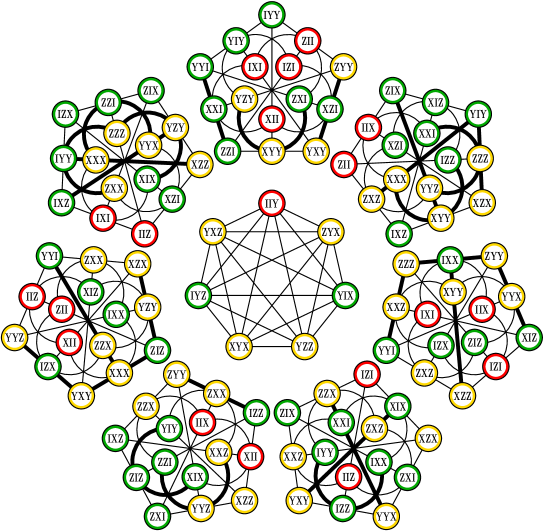
Figure 4: An illustration of the structure of the three-qubit hyperbolic quadric $\mathcal{Q}_{0}$ in terms of seven doilies that pairwise share an elliptic quadric. There are shown all 105 lines (each belonging to a unique doily) and all 35 points (each occurring in three different doilies) of the quadric. Due to the lack of space, we use a shorthand notation $ABC$ instead of $A\otimes B\otimes C$ for the 63 canonical elements of $P_{3}/C_{3}$. The elements themselves are further distinguished by different colors according as they feature two $I$’s (red), one $I$ (green) aor no $I$ (yellow). The negative lines/contexts are boldfaced. The seven elements labeling the vertices of the central heptagon correspond to a particular Conwell heptad of points lying off $\mathcal{Q}_{0}$ (for more details, see [SdBHG21]).

The degree of contextuality can be obtained by counting the minimal number of constraints that cannot be satisfied by an NCHV model. It is always possible to satisfy the constraints imposed by the $78$ positive lines of $\mathcal{Q}_{0}$ but the question of satisfying part of the constraints imposed by the $27$ negative lines is more subtle. The degree of contextuality of $W_{2}$ being $3$, Fig. 4 implies that $7\times 3=21$ constraints cannot be satisfied which corresponds exactly to the degree of contextuality of $\mathcal{Q}_{0}$.

In the case of the elliptic quadric one can also give a nice justification of the fact that their degree of contextuality is $9$ in $W_{3}$. Let us denote by $\mathcal{Q}^{\prime}$ such an elliptic quadric in $W_{3}$, i.e. the zero locus of an elliptic quadratic form, see Sect. 5. It is known that $\mathcal{Q}^{\prime}$, as a point-line geometry, is a generalized quadrangle $GQ(2,4)$, i.e. a point-line configuration of $3$ points per line and $5$ lines per point which is triangle-free [SGL⁺10, LSVP09]. The configuration is made of $27$ points and $45$ lines. As shown in [LSVP09], out of those $45$ lines one can build $36$ doilies such that every line shows up in $12$ different doilies. But again one knows that in each doily there are always $3$ constraints that cannot be satisfied because the degree of contextuality of $W_{2}$ is $3$. Therefore the number of constraints of $GQ(2,4)$ that cannot be satisfied is $36\times 3/12=9$, which is the degree computed in Sect. 6.

To conclude this section, let us emphasize some practical information that the knowledge of the contextual degree provides for experimental testing of quantum contextuality. Beside the upper bound, $b$, for contextual inequalities discussed in Sect. 3, let us discuss what Cabello defines in [Cab10] as a measure of robustness of a quantum violation of the non-contextual inequality Eq. (6). This notion of tolerated error per context is expressed as

$$\varepsilon=\frac{N-b}{N}=\frac{2d}{N},$$ (8)

where $N$ is the number of contexts of the configuration, $b$ is the upper bound of Eq. (6) of an NCHV model and $d$ is the degree of contextuality. The tolerated error per context $\varepsilon$ measures the errors that can occur, on each context, due to experimental imperfection, while still violating the corresponding contextual inequality based on the configuration. Thanks to the results obtained in this paper, we can establish Tab. 4, that can be compared to Tab. I of [TLC22]. One observes that the ratio $b/N$ and the tolerated error per context are as good as the best contextual scenario proposed in Tab. I of [TLC22].

Configuration	Observables	Contexts	$b/N$	$\varepsilon$
Hyperbolic quadric	$35$	$105$	$63/105=0.6$	$0.4$
Elliptic quadric	$27$	$45$	$27/45=0.6$	$0.4$

Table 4: Characteristics for experimental implementations of contextual inequalities based on $3$-qubit quadrics.

From an experimental perspective, in order to obtain a violation of Eq. (6) we would like to have the smallest possible ratio $\frac{b}{N}$ and the biggest value $\varepsilon$. In this respect both hyperbolic and elliptic quadrics are as good as the Mermin pentagram which has a smaller ratio $\frac{b}{N}$ and a bigger tolerated error $\varepsilon$ per context than the new magic sets of [TLC22].

7 Smallest split Cayley hexagons in $W_{3}$

A particularly nice illustration of the power and physical relevance of our contextuality algorithm is provided by another notable finite geometry living in $W_{3}$, namely the split Cayley hexagon of order two, $\mathcal{H}$. Being a generalized polygon like the doily itself (see, e. g., [PSvM01]), it is a point-line incidence structure featuring 63 points and 63 lines, with three points on a line and three lines through a point, whose group of automorphisms is isomorphic to $G_{2}(2)$ of order $12\,096$. As it was first shown by Coolsaet [Coo10], $\mathcal{H}$ can be embedded into $W_{3}$ in two fundamentally different ways, called classical ($\mathcal{H}_{C}$; 120 distinct copies) and skew ($\mathcal{H}_{S}$; 7560 copies). In a recent paper [HdBS22], three of us employed the present algorithm to ascertain contextuality properties of each of these three-qubit embedded split Cayley hexagons. The authors were quite surprised to find out that although neither an $\mathcal{H}_{C}$ nor an $\mathcal{H}_{S}$ is contextual, this is not the case with their line-complements, $\overline{\mathcal{H}}$’s (note that $\mathcal{H}$ and $\overline{\mathcal{H}}$ are identical as point-sets); indeed, it was found that an $\overline{\mathcal{H}_{C}}$ is non-contextual, whereas any $\overline{\mathcal{H}_{S}}$ is! So, this is the first stance of a quantum geometry ever discovered where it is not so much the (properties of the) geometry of its own, but rather the way how it embeds into the ambient multi-qubit symplectic polar space that matters when it comes to quantum contextuality issues. Moreover, given the fact that $\overline{\mathcal{H}_{S}}$’s exhibit a considerable smaller degree of symmetry than $\overline{\mathcal{H}_{C}}$’s, this finding also seems to indicate that in our future quest(s) for other examples of contextual configurations one should pay a particular attention to those finite geometries that are not so symmetry-pronounced.

8 Conclusion

In this paper we performed a systematic computer-aided study of observable-based proofs of contextuality with large numbers of contexts and observables as subgeometries of the symplectic polar space $W_{n}$. We generate in particular (in Sect. 5) new proofs based on hyperbolic and elliptic quadrics for $n=3,4,5$. Moreover, we quantified contextuality through the notion of contextuality degree and we computed this degree for these new proofs, in the $n=3$ case.

A natural generalization would be to prove that quadrics are always point-line configurations that provide observable-based proofs of the Kochen-Specker Theorem for any $n$. The fact that for $n=3$ we were able to compute the degree of contextuality for both $\mathcal{Q}_{0}$, hyperbolic quadric, and $\mathcal{Q}^{\prime}$, elliptic quadric, by geometric partition of the lines in terms of doilies can be considered as a concrete motivation for studying how doilies cover $W_{n}$ and its subspaces. In this respect our work on the taxonomy of the symplectic polar spaces by means of $W_{2}$ [SdBHG21] can be used to estimate the degree of contextuality for subgeometries of $W_{n}$. Those questions will be addressed in a future work.

References

- [AB11] S. Abramsky and A. Brandenburger. The sheaf-theoretic structure of non-locality and contextuality. New Journal of Physics, 13(11):113036, November 2011. https://doi.org/10.1088/1367-2630/13/11/113036.
- [ABCP17] S. Abramsky, R. S. Barbosa, G. Carù, and S. Perdrix. A complete characterisation of All-versus-Nothing arguments for stabiliser states. Philosophical Transactions of the Royal Society A: Mathematical, Physical and Engineering Sciences, 375(2106):20160385, November 2017. http://arxiv.org/abs/1705.08459.
- [AC16] S. Abramsky and G. Caru. Identifying All-vs-Nothing Arguments in Stabiliser Theory. In Quantum Physics and Logic, page 12, 2016.
- [ARBC09] E. Amselem, M. Rådmark, M. Bourennane, and A. Cabello. State-independent quantum contextuality with single photons. Physical Review Letters, 103(16):160405, October 2009.
- [Ark12] A. Arkhipov. Extending and Characterizing Quantum Magic Games. arXiv:1209.3819 [quant-ph], September 2012. http://arxiv.org/abs/1209.3819.
- [BBT05] G. Brassard, A. Broadbent, and A. Tapp. Quantum Pseudo-Telepathy. Foundations of Physics, 35(11):1877–1907, November 2005. https://doi.org/10.1007/s10701-005-7353-4.
- [Bel64] J. S. Bell. On the Einstein Podolsky Rosen paradox. Physics, 1(3):195–200, 1964.
- [Bel66] J. S. Bell. On the Problem of Hidden Variables in Quantum Mechanics. Reviews of Modern Physics, 38(3):447–452, July 1966. https://link.aps.org/doi/10.1103/RevModPhys.38.447.
- [Cab08] A. Cabello. Experimentally testable state-independent quantum contextuality. Physical Review Letters, 101(21):210401, November 2008. http://arxiv.org/abs/0808.2456.
- [Cab10] A. Cabello. Proposed test of macroscopic quantum contextuality. Physical Review A, 82(3):032110, September 2010. https://link.aps.org/doi/10.1103/PhysRevA.82.032110.
- [CEGA96] A. Cabello, J. M. Estebaranz, and G. García-Alcaine. Bell-Kochen-Specker theorem: A proof with 18 vectors. Physics Letters A, 212(4):183–187, March 1996. http://www.sciencedirect.com/science/article/pii/037596019600134X.
- [CM13] R. Cleve and R. Mittal. Characterization of Binary Constraint System Games. arXiv:1209.2729 [quant-ph], October 2013. http://arxiv.org/abs/1209.2729.
- [Coo10] K. Coolsaet. The smallest split Cayley hexagon has two symplectic embeddings. Finite Fields and Their Applications, 16(5):380–384, September 2010. https://www.sciencedirect.com/science/article/pii/S1071579710000572.
- [dBHG+22] H. de Boutray, F. Holweck, A. Giorgetti, P. Masson, and M. Saniga. Contextuality degree of quadrics in multi-qubit symplectic polar spaces. Journal of Physics A: Mathematical and Theoretical, 55(47):475301, November 2022. https://dx.doi.org/10.1088/1751-8121/aca36f.
- [DRLB20] A. Dikme, N. Reichel, A. Laghaout, and G. Björk. Measuring the Mermin-Peres magic square using an online quantum computer. arXiv:2009.10751 [quant-ph], September 2020. http://arxiv.org/abs/2009.10751.
- [HdBS22] F. Holweck, H. de Boutray, and M. Saniga. Three-qubit-embedded split Cayley hexagon is contextuality sensitive. Scientific Reports, 12(1):8915, May 2022. https://www.nature.com/articles/s41598-022-13079-3.
- [Hol21] F. Holweck. Testing Quantum Contextuality of Binary Symplectic Polar Spaces on a Noisy Intermediate Scale Quantum Computer. Quantum Information Processing, January 2021. http://arxiv.org/abs/2101.03812.
- [HS17] F. Holweck and M. Saniga. Contextuality with a Small Number of Observables. International Journal of Quantum Information, 15(04):1750026, June 2017. http://arxiv.org/abs/1607.07567.
- [HWVE14] M. Howard, J. J. Wallman, V. Veitch, and J. Emerson. Contextuality supplies the magic for quantum computation. Nature, 510(7505):351–355, June 2014. http://arxiv.org/abs/1401.4174.
- [KS67] S. Kochen and E. Specker. The Problem of Hidden Variables in Quantum Mechanics. Journal of Mathematics and Mechanics, 17(1):59–87, 1967. https://www.jstor.org/stable/24902153.
- [KZG+09] G. Kirchmair, F. Zähringer, R. Gerritsma, M. Kleinmann, O. Gühne, A. Cabello, R. Blatt, and C. F. Roos. State-independent experimental test of quantum contextuality. Nature, 460(7254):494–497, July 2009. http://arxiv.org/abs/0904.1655.
- [LHS17] P. Lévay, F. Holweck, and M. Saniga. Magic three-qubit Veldkamp line: A finite geometric underpinning for form theories of gravity and black hole entropy. Physical Review D, 96(2):026018, July 2017. https://link.aps.org/doi/10.1103/PhysRevD.96.026018.
- [LS17] P. Lévay and Z. Szabó. Mermin pentagrams arising from Veldkamp lines for three qubits. Journal of Physics A: Mathematical and Theoretical, 50(9):095201, January 2017. https://doi.org/10.1088/1751-8121/aa56aa.
- [LSVP09] P. Lévay, M. Saniga, P. Vrana, and P. Pracna. Black hole entropy and finite geometry. Physical Review D, 79(8):084036, April 2009. https://link.aps.org/doi/10.1103/PhysRevD.79.084036.
- [Mer93] N. D. Mermin. Hidden variables and the two theorems of John Bell. Reviews of Modern Physics, 65(3):803–815, July 1993. https://link.aps.org/doi/10.1103/RevModPhys.65.803.
- [MSG+22] A. Muller, M. Saniga, A. Giorgetti, H. De Boutray, and F. Holweck. Multi-qubit doilies: Enumeration for all ranks and classification for ranks four and five. http://arxiv.org/abs/2206.03599, June 2022.
- [ORBR17] C. Okay, S. Roberts, S. D. Bartlett, and R. Raussendorf. Topological proofs of contextuality in quantum mechanics. arXiv:1701.01888 [quant-ph], October 2017. http://arxiv.org/abs/1701.01888.
- [Per90] A. Peres. Incompatible results of quantum measurements. Physics Letters A, 151(3):107–108, December 1990. https://www.sciencedirect.com/science/article/pii/037596019090172K.
- [Pla12] M. Planat. On small proofs of the Bell-Kochen-Specker theorem for two, three and four qubits. The European Physical Journal Plus, 127(8):86, August 2012. https://doi.org/10.1140/epjp/i2012-12086-x.
- [PSH13] M. Planat, M. Saniga, and F. Holweck. Distinguished three-qubit ‘magicity’ via automorphisms of the split Cayley hexagon. Quantum Information Processing, 12(7):2535–2549, July 2013. https://doi.org/10.1007/s11128-013-0547-3.
- [PSvM01] B. Polster, A. E. Schroth, and H. van Maldeghem. Generalized Flatland. The Mathematical Intelligencer, 23(4):33–47, September 2001. https://doi.org/10.1007/BF03024601.
- [Rau13] R. Raussendorf. Contextuality in Measurement-based Quantum Computation. Physical Review A, 88(2):022322, August 2013. http://arxiv.org/abs/0907.5449.
- [San19] M. Saniga. Doily – A Gem of the Quantum Universe. https://www.astro.sk/~msaniga/pub/ftp/bled.pdf, June 2019.
- [SdBHG21] M. Saniga, H. de Boutray, F. Holweck, and A. Giorgetti. Taxonomy of Polar Subspaces of Multi-Qubit Symplectic Polar Spaces of Small Rank. Mathematics, 9(18):2272, September 2021. https://www.mdpi.com/2227-7390/9/18/2272.
- [SGL+10] M. Saniga, R. M. Green, P. Lévay, P. Pracna, and P. Vrana. The Veldkamp Space of GQ(2,4). International Journal of Geometric Methods in Modern Physics, 07(07):1133–1145, November 2010. http://arxiv.org/abs/0903.0715.
- [SPPH07] M. Saniga, M. Planat, P. Pracna, and H. Havlicek. The Veldkamp Space of Two-Qubits. SIGMA. Symmetry, Integrability and Geometry: Methods and Applications, 3:075, June 2007. http://www.emis.de/journals/SIGMA/2007/075/.
- [TLC22] S. Trandafir, P. Lisoněk, and A. Cabello. Irreducible magic sets for -qubit systems. arXiv:2202.13141 [quant-ph], February 2022. http://arxiv.org/abs/2202.13141.
- [VL10] P. Vrana and P. Lévay. The Veldkamp space of multiple qubits. Journal of Physics A: Mathematical and Theoretical, 43(12):125303, March 2010. https://doi.org/10.1088/1751-8113/43/12/125303.
- [WA11] M. Waegell and P. K. Aravind. Parity Proofs of the Kochen-Specker Theorem Based on the 24 Rays of Peres. Foundations of Physics, 41(12):1786–1799, December 2011. https://doi.org/10.1007/s10701-011-9578-8.