Parametric dependence of bound states in the continuum
in periodic structures: vectorial cases

Abstract

A periodic structure sandwiched between two homogeneous media can support bound states in the continuum (BICs) that are valuable for many applications. It is known that generic BICs in periodic structures with an up-down mirror symmetry and an in-plane inversion symmetry are robust with respect to structural perturbations that preserve these two symmetries. For two-dimensional (2D) structures with one periodic direction and the up-down mirror symmetry (without the in-plane inversion symmetry), it was recently established that some scalar BICs can be found by tuning a single structural parameter. In this paper, we analyze vectorial BICs in such 2D structures, and show that a typical vectorial BIC with nonzero wavenumbers in both the invariant and the periodic directions can only be found by tuning two structural parameters. Using an all-order perturbation method, we prove that such a vectorial BIC exists as a curve in the 3D space of three generic parameters. Our theory is validated by numerical examples involving periodic arrays of dielectric cylinders. The numerical results also illustrate the conservation of topological charge when structural parameters are varied, if both BICs and circularly polarized states (CPSs) are included. Our study reveals a fundamental property of BICs in periodic structure and provides a systematically approach for finding BICs in structures with less symmetry.

I Introduction

Due to their intriguing properties and valuable applications, photonic bound state in the continuum (BICs) have been extensively studied in recent years hsu16 ; kosh19 ; azzam . In a lossless structure that is invariant or periodic in one or two spatial directions, a BIC is a special resonant state with an infinite quality factor ($Q$ factor) bonnet94 ; port05 ; mari08 ; plot11 ; hsu13_2 ; bulg14 ; zou15 ; gomis17 , and it gives high-$Q$ resonances when the structure or the wavevector is perturbed kosh18 ; hu18 ; lijun20 ; taghi17 ; rybin17 ; lijun18pra ; jin19 ; zhen20b ; huyuan19 . The BICs have found important applications include lasing kodi17 , sensing yesi19 , harmonic generation kosh20 , low-refractive-index light guiding zou15 ; yu19 , etc. The BICs in periodic structures exhibit interesting topological properties. The topological charge of a BIC can be defined using the far-field major polarization vector zhen14 ; bulg17pra . If a BIC with a nonzero topological charge is destroyed by a perturbation, circularly polarized states (CPSs) emerge and the net topological charge remains unchanged liu20 ; yoda20 ; amgad21 .

Although a BIC typically becomes a high-$Q$ resonance when the structure is perturbed kosh18 ; hu18 ; lijun20 , it may persist if the perturbation satisfies certain conditions. If a BIC is protected by a symmetry bonnet94 ; padd00 ; ochiai01 ; tikh02 ; shipman03 ; lee12 , it naturally continues to exist when the perturbation preserves the symmetry. In periodic structures sandwiched between two homogeneous media, there are propagating BICs with a nonzero wavevector port05 ; mari08 ; hsu13_2 ; bulg14 ; yang14 ; gan16 . These BICs are not protected by symmetry in the usual sense, but they are robust with respect to structural perturbations that maintain the relevant symmetry zhen14 ; yuan17ol ; yuan21 . Even for perturbations without any symmetry, a BIC is not always destroyed. In a recent work yuan20_2 , we studied the continual existence of scalar BICs in periodic structures without the in-plane inversion symmetry. We showed that for a generic perturbation with two parameters, a scalar BIC (with a frequency such that there is only one radiation channel) can be maintained by tuning one parameter. This implies that a typical scalar BIC exists on a curve in the plane of two generic parameters.

Our previous work is limited to scalar $E$-polarized BICs yuan20_2 . In a 2D structure that is invariant in $x$ and periodic in $y$, a BIC is associated with wavenumbers $\alpha$ and $\beta$ corresponding to the $x$ and $y$ directions, respectively. When $\alpha=0$, the BIC is a scalar one and it can be either $E$-polarized or $H$-polarized. The case $\alpha\neq 0$ corresponds to a vectorial BIC bulg17pra . In this paper, we analyze the parametric dependence for vectorial BICs in 2D periodic structures. It turns out that the vectorial BICs for $\beta=0$ and $\beta\neq 0$ exhibit different behavior in parameter space. Similar to the scalar BICs, a vectorial BIC with $\beta=0$ exists as a curve in the plane of two generic structural parameters. On the other hand, a vectorial BIC with $\beta\neq 0$ appears as an isolated point in the plane of two parameters, but exists as a curve in the space of three generic parameters. This distinction between the two types of vectorial BICs is somewhat unexpected, since when the periodic structure has the in-plane inversion symmetry, they are both robust.

The rest of this paper is organized as follows. In Sec. II, we briefly describe the structure, the BICs and related diffraction solutions. In Sec. III, we give an outline for a proof that characterizes the dependence of BICs on structural parameters. In Sec. IV, we present numerical examples to validate the theory and demonstrate the emergence and annihilation of CPSs when BICs are destroyed or created. The paper is concluded with some remarks in Sec. V.

II BICs and diffraction solutions

We consider a 2D lossless dielectric structure that is invariant in $x$, periodic in $y$ with period $L$, and symmetric in $z$ (i.e. the up-down mirror symmetry). The dielectric function is real and satisfies

$$\varepsilon({\bm{r}})=\varepsilon(y+L,z)=\varepsilon(y,-z)$$ (1)

for all ${\bm{r}}=(y,z)$. It is also assumed that the periodic layer is sandwiched between two identical homogeneous media with a dielectric constant $\varepsilon_{0}\geq 1$. Therefore,

$$\varepsilon({\bm{r}})=\varepsilon_{0},\quad\mbox{for}\ |z|>d,$$ (2)

where $d$ is a positive constant.

Since the structure is invariant in $x$, we consider a general eigenmode that depends on $x$ and time $t$ as $\exp[i(\alpha x-\omega t)]$, where $\alpha$ is a real wavenumber for the $x$ direction and $\omega$ is the angular frequency. The electric field is the real part of ${\bm{E}}({\bm{r}})e^{i(\alpha x-\omega t)}$, where ${\bm{E}}$ satisfies

$$\left(\nabla+i\alpha{\bm{e}}_{1}\right)\times\left(\nabla+i\alpha{\bm{e}}_{1}\right)\times{\bm{E}}-k^{2}\varepsilon({\bm{r}}){\bm{E}}=0,$$ (3)

$$\left(\nabla+i\alpha{\bm{e}}_{1}\right)\cdot[\varepsilon({\bm{r}}){\bm{E}}]=0,$$ (4)

$k=\omega/c$ is the freespace wavenumber, $c$ is the speed of light in vacuum, and ${\bm{e}}_{1}=(1,0,0)$ is the unit vector in the $x$ direction. Due to the periodicity in $y$, the eigenmode can be written as

$${\bm{E}({\bm{r}})}={\bm{\Phi}}({\bm{r}})e^{i\beta y},$$ (5)

where ${\bm{\Phi}}({\bm{r}})$ is periodic in $y$ with period $L$, and $\beta$ is the Bloch wavenumber in $y$ satisfying $|\beta|\leq\pi/L$.

A BIC is a special guided mode with a real wavevector $(\alpha,\beta)$ and a real frequency $\omega$ satisfying $\sqrt{\alpha^{2}+\beta^{2}}<k\sqrt{\varepsilon_{0}}$. The electric field of the BIC satisfies ${\bm{E}}({\bm{r}})\to{\bm{0}}$ as $z\to\pm\infty$ and is normalized such that

$$\dfrac{1}{L^{2}}\int_{\Omega}\varepsilon({\bm{r}})\overline{{\bm{E}}}({\bm{r}})\cdot{\bm{E}}({\bm{r}})\,d{\bm{r}}=1,$$ (6)

where $\overline{\bm{E}}$ is the complex conjugate of ${\bm{E}}$, and $\Omega=\left\{(y,z):|y|<L/2,|z|<+\infty\right\}$ is one period of the cross section of the structure. If the BIC is non-degenerate and its electric field is ${\bm{E}}({\bm{r}})=\left[E_{x}({\bm{r}}),E_{y}({\bm{r}}),E_{z}({\bm{r}})\right]$, we can define a vector field $\tilde{\bm{E}}$ by

$$\tilde{{\bm{E}}}({\bm{r}})=\left[E_{x}(y,-z),E_{y}(y,-z),-E_{z}(y,-z)\right].$$ (7)

Since $\tilde{\bm{E}}$ is also a BIC for the same frequency and the same wavevector, we can scale the BIC such that either

$${\bm{E}}({\bm{r}})=\tilde{{\bm{E}}}({\bm{r}}),\quad\mbox{or}$$ (8)

$${\bm{E}}({\bm{r}})=-\tilde{{\bm{E}}}({\bm{r}}).$$ (9)

In the homogeneous media above or below the periodic layer, plane waves compatible with the BIC have wavevectors $(\alpha,\beta_{m},\pm\gamma_{m})$, where

$$\beta_{m}=\beta+\frac{2\pi m}{L},\quad\gamma_{m}=\sqrt{k^{2}\varepsilon_{0}-\alpha^{2}-\beta_{m}^{2}}.$$ (10)

In this paper, we only consider BICs satisfying

$$\sqrt{\alpha^{2}+\beta^{2}}<k\sqrt{\varepsilon_{0}}<\sqrt{\alpha^{2}+\left(\frac{2\pi}{L}-|\beta|\right)^{2}}.$$ (11)

The above condition implies that $\gamma=\gamma_{0}>0$ and all other $\gamma_{m}$ for $m\neq 0$ are pure imaginary. Therefore, the only propagating plane waves are those with wavevectors $(\alpha,\beta,\pm\gamma)$. This ensures that only one radiation channel is open in each side of the periodic layer. Moreover, the symmetry condition (8) or (9) implies the radiation channels above and below the periodic layer can be regarded as one channel.

In the process of proving our main result, we need diffraction solutions having the same symmetry in $z$ as the BIC. Given the real wavevector ${\bm{k}}=(\alpha,\beta,\gamma)$, we have two real unit vectors ${\bm{f}}_{1}$ and ${\bm{f}}_{2}$ such that $\{{\bm{k}},{\bm{f}}_{1},{\bm{f}}_{2}\}$ is an orthogonal set. If the BIC satisfies condition (8), we can construct two diffraction solutions ${\bm{E}}_{1}^{(s)}$ and ${\bm{E}}_{2}^{(s)}$ that also satisfy condition (8). If ${\bm{f}}_{1}=(f_{1x},f_{1y},f_{1z})$, then ${\bm{E}}_{1}^{(s)}$ is the solution with incident plane waves

$$(f_{1x},f_{1y},\pm f_{1z})e^{i(\beta y\pm\gamma z)}$$

given below and above the periodic layer (i.e. for $z<-d$ and $z>d$), respectively. Note that we can define a vector field $\tilde{\bm{E}}^{(s)}_{1}$ from ${\bm{E}}_{1}^{(s)}$ following Eq. (7), then $({\bm{E}}_{1}^{(s)}+\tilde{\bm{E}}_{1}^{(s)})/2$ solves the same diffraction problem and clearly satisfies condition (8). Similarly, using the vector ${\bm{f}}_{2}$, we can construct a diffraction solution ${\bm{E}}_{2}^{(s)}$ satisfying condition (8). The case for condition (9) is similar.

When there is a BIC, the related diffraction problem does not have a unique solution. For any constant $C_{0}$, ${\bm{E}}_{j}^{(s)}+C_{0}{\bm{E}}$ (for $j=1$, 2) solves the same diffraction problem as ${\bm{E}}_{j}^{(s)}$. Without loss of generality, we assume the diffraction solutions are orthogonal with the BIC, i.e.,

$$\int_{\Omega}\varepsilon({\bm{r}})\overline{{\bm{E}}}^{(s)}_{j}\cdot{\bm{E}}\,d{\bm{r}}=0,\quad j=1,2.$$ (12)

If the Bloch wavenumber $\beta$ of the BIC is zero, then the vector field given by

$$\hat{{\bm{E}}}({\bm{r}})=\left[-\overline{E}_{x}({\bm{r}}),\overline{E}_{y}({\bm{r}}),\overline{E}_{z}({\bm{r}})\right]$$ (13)

is also a BIC with the same $\alpha$, $\beta=0$ and $\omega$. Since we assume the BIC is non-degenerate, there must be a constant $C_{1}$ such that $\hat{{\bm{E}}}=C_{1}{\bm{E}}$. Since the power carried by the BIC is finite, $C_{1}$ must satisfy $|C_{1}|=1$. If $C_{1}=e^{2i\varphi}$ for a real $\varphi$, we can replace ${\bm{E}}$ by $e^{i\varphi}{\bm{E}}$, then the new ${\bm{E}}$ satisfies

$${\bm{E}}({\bm{r}})=\hat{{\bm{E}}}({\bm{r}}).$$ (14)

This implies that $E_{y}$ and $E_{z}$ are real and $E_{x}$ is pure imaginary. Similarly, the diffraction solutions ${\bm{E}}_{1}^{(s)}$ and ${\bm{E}}_{2}^{(s)}$ can also be scaled to satisfy condition (14).

III Parametric dependence

Our objective is to understand how a typical BIC depends on structural parameters. In general, the dielectric function of a 2D periodic structure, denoted as $\varepsilon_{\rm g}({\bm{r}};{\bm{p}})$, may depend on a vector ${\bm{p}}=(p_{1},p_{2},...,p_{m})$ for $m$ real parameters. If there is a non-degenerate BIC in the structure when ${\bm{p}}={\bm{p}}_{*}$, we aim to find those ${\bm{p}}$ near ${\bm{p}}_{*}$, such that the BIC continues to exist. Typically, in the $m$-dimensional parameter space, the values of ${\bm{p}}$ for which the BIC exists form a geometric object with a dimension less than $m$. For scalar $E$-polarized BICs, we have previously proved that the dimension the geometric object is actually $m-1$, i.e. the codimension of the geometric object is one yuan20_2 . In the following, we show that for vectorial BICs with $\beta=0$ and $\beta\neq 0$, the codimension is one and two, respectively.

For the case of codimension-$1$, it is sufficient to consider two parameters, i.e., $m=2$. In addition, for ${\bm{p}}$ near ${\bm{p}}_{*}$, a general two-parameter real dielectric function $\varepsilon_{\rm g}({\bm{r}};{\bm{p}})$ can be approximated by

$$\varepsilon({\bm{r}})=\varepsilon_{*}({\bm{r}})+\delta G({\bm{r}})+\eta F({\bm{r}}),$$ (15)

where $\varepsilon_{*}({\bm{r}})=\varepsilon_{\rm g}({\bm{r}};{\bm{p}}_{*})$, ${\bm{p}}_{*}=(p_{1*},p_{2*})$, $\delta=p_{1}-p_{1*}$, $\eta=p_{2}-p_{2*}$, $G({\bm{r}})$ and $F({\bm{r}})$ are partial derivatives of $\varepsilon_{\rm g}$ (evaluated at ${\bm{p}}_{*}$) with respect to $p_{1}$ and $p_{2}$, respectively. We assume $\varepsilon_{*}({\bm{r}})$ satisfies conditions (1) and (2), $F({\bm{r}})$ and $G({\bm{r}})$ satisfy condition (1) and vanish for $|z|>d$. For the case of codimension-$2$, if $\varepsilon({\bm{r}})$ is still given by Eq. (15), then in general no BICs can be found for $(\delta,\eta)$ near $(0,0)$. Therefore, we have to introduce three parameters ($m=3$) and replace Eq. (15) by

$$\varepsilon({\bm{r}})=\varepsilon_{*}({\bm{r}})+\delta G({\bm{r}})+\eta F({\bm{r}})+sP({\bm{r}}),$$ (16)

where $s=p_{3}-p_{3*}$, $P({\bm{r}})=\partial\varepsilon_{g}/\partial p_{3}|_{{\bm{p}}={\bm{p}}_{*}}$, and $P({\bm{r}})$ satisfies condition (1) and is zero if $|z|>d$. Assuming a BIC exists in the unperturbed structure, we need to show that for any real $\delta$ near zero, there is a real $\eta$ (and a real $s$), such that the BIC continues its existence in the perturbed structure given by Eq. (15) or Eq. (16).

We assume the unperturbed structure with the dielectric function $\varepsilon_{*}({\bm{r}})$ has a non-degenerate BIC with a frequency $\omega_{*}$, a wavevector $(\alpha_{*},\beta_{*})$, and an electric field ${\bm{E}}_{*}({\bm{r}})={\bm{\Phi}}_{*}({\bm{r}})e^{i\beta_{*}y}$. We also assume the triple $(\alpha_{*},\beta_{*},\omega_{*})$ satisfies condition (11) and the BIC satisfies Eq. (8). Let the diffraction solutions corresponding to the BIC, as introduced in Sec. II, be ${\bm{E}}_{j}^{(s)}({\bm{r}})={\bm{\Psi}}_{j}({\bm{r}})e^{i\beta_{*}y}$ for $j=1$, 2. We assume they satisfy Eqs. (8) and (12). For the perturbed structure given by Eq. (15) or Eq. (16), we look for a BIC, near the one in the unperturbed structure, with a frequency $\omega$, a wavevector $(\alpha,\beta)$, and electric field ${\bm{E}}({\bm{r}})={\bm{\Phi}}({\bm{r}})e^{i\beta y}$.

First, we establish a codimension-$2$ result for vectorial BICs with $\alpha_{*}\neq 0$ and $\beta_{*}\neq 0$. For a perturbed structure with $\varepsilon({\bm{r}})$ given in Eq. (16), a BIC, if it exists, can be found by expanding ${\bm{\Phi}}$, $\alpha$, $\beta$, $k$, $\eta$ and $s$ in power series of $\delta$:

$${\bm{\Phi}} = {\bm{\Phi}}_{*}+{\bm{\Phi}}_{1}\delta+{\bm{\Phi}}_{2}\delta^{2}+\cdots$$ (17)

$$\alpha = \alpha_{*}+\alpha_{1}\delta+\alpha_{2}\delta^{2}+\cdots$$ (18)

$$\beta = \beta_{*}+\beta_{1}\delta+\beta_{2}\delta^{2}+\cdots$$ (19)

$$k = k_{*}+k_{1}\delta+k_{2}\delta^{2}+\cdots$$ (20)

$$\eta = \quad\quad\eta_{1}\delta+\eta_{2}\delta^{2}+\cdots$$ (21)

$$s = \quad\quad s_{1}\delta+s_{2}\delta^{2}+\cdots$$ (22)

Here, $\delta$ is a small and arbitrary real number, $\eta$ and $s$ depend on $\delta$ and are also expanded. Inserting the above into the governing equations for ${\bm{\Phi}}$, i.e., Eqs. (A1) and (A2) in the Appendix, and comparing the coefficients of $\delta^{j}$ for each $j\geq 1$, we obtain the following differential equation for ${\bm{\Phi}}_{j}$:

$$\mathcal{L}{\bm{\Phi}}_{j}=\alpha_{j}\mathcal{B}_{1}{\bm{\Phi}}_{*}+\beta_{j}\mathcal{B}_{2}{\bm{\Phi}}_{*}+2k_{*}k_{j}\varepsilon_{*}{\bm{\Phi}}_{*}$$

$$\qquad+k_{*}^{2}\eta_{j}F({\bm{r}}){\bm{\Phi}}_{*}+k_{*}^{2}s_{j}P({\bm{r}}){\bm{\Phi}}_{*}+{\bm{C}}_{j}({\bm{r}}),$$ (23)

$$(\nabla+i{\bm{\alpha}}_{*})\cdot(\varepsilon_{*}{\bm{\Phi}}_{j})=\alpha_{j}h_{1}({\bm{r}})+\beta_{j}h_{2}({\bm{r}})$$

$$\qquad+\eta_{j}h_{3}({\bm{r}})+s_{j}h_{4}({\bm{r}})+g_{j}({\bm{r}}),$$ (24)

where ${\bm{\alpha}}_{*}=(\alpha_{*},\beta_{*},0)$, ${\cal L}$, ${\cal B}_{1}$, ${\cal B}_{2}$ are differential operators, $h_{m}$ (for $m=1$, 2, 3, 4) are scalar functions depending on $\alpha_{*}$, $\beta_{*}$, $k_{*}$ and $\varepsilon_{*}({\bm{r}})$, ${\bm{C}}_{j}$ is a vector field and $g_{j}$ is a scalar function depending on all previous iterations such as ${\bm{\Phi}}_{m}$ for $m<j$. The details are given in the Appendix. Importantly, the BIC exists if and only if, for each $j\geq 1$, $\alpha_{j}$, $\beta_{j}$, $k_{j}$, $\eta_{j}$ and $s_{j}$ can be solved and they are real, and ${\bm{\Phi}}_{j}$ can be solved from Eqs. (III) and (III) and it decays exponentially to zero as $|z|\to\infty$.

Integrating the dot products of Eq. (III) with the complex conjugates of ${\bm{\Phi}}_{*}$, ${\bm{\Psi}}_{1}$ and ${\bm{\Psi}}_{2}$ on $\Omega$, we obtain a $3\times 5$ linear system

$$\left[\begin{matrix}a_{11}&a_{12}&a_{13}&a_{14}&a_{15}\cr a_{21}&a_{22}&0&a_{24}&a_{25}\cr a_{31}&a_{32}&0&a_{34}&a_{35}\end{matrix}\right]\left[\begin{matrix}\alpha_{j}\cr\beta_{j}\cr k_{j}\cr\eta_{j}\cr s_{j}\end{matrix}\right]=\left[\begin{matrix}{b}_{1j}\cr{b}_{2j}\cr{b}_{3j}\end{matrix}\right]$$ (25)

with a $3\times 5$ coefficient matrix ${\bm{A}}$ and a right hand side ${\bm{b}}_{j}$. The entries of ${\bm{A}}$ and ${\bm{b}}_{j}$ are given in the Appendix. While Eq. (25) is a necessary condition for Eq. (III) to have a solution that decays exponentially to zero as $|z|\to\infty$, it is also a sufficient condition. More precisely, if all previous iterations ${\bm{\Phi}}_{m}$ for $m<j$ decay to zero exponentially as $|z|\to\infty$, and $(\alpha_{j},\beta_{j},k_{j},\eta_{j},s_{j})$ is a real solution of Eq. (25), then Eq. (III) always has a solution that decays to zero exponentially as $|z|\to\infty$. It is easy to show that all entries in the first row of matrix ${\bm{A}}$ and $b_{1j}$ are real, thus, Eq. (25) is equivalent to the following real $5\times 5$ linear system:

$$\left[\begin{matrix}a_{11}&a_{12}&a_{13}&a_{14}&a_{15}\cr a^{\prime}_{21}&a^{\prime}_{22}&0&a^{\prime}_{24}&a^{\prime}_{25}\cr a^{\prime}_{31}&a^{\prime}_{32}&0&a^{\prime}_{34}&a^{\prime}_{35}\cr a^{\prime\prime}_{21}&a^{\prime\prime}_{22}&0&a^{\prime\prime}_{24}&a^{\prime\prime}_{25}\cr a^{\prime\prime}_{31}&a^{\prime\prime}_{32}&0&a^{\prime\prime}_{34}&a^{\prime\prime}_{35}\end{matrix}\right]\left[\begin{matrix}\alpha_{j}\cr\beta_{j}\cr k_{j}\cr\eta_{j}\cr s_{j}\end{matrix}\right]=\left[\begin{matrix}{b}_{1j}\cr b^{\prime}_{2j}\cr b^{\prime}_{3j}\cr b^{\prime\prime}_{2j}\cr b^{\prime\prime}_{3j}\end{matrix}\right],$$ (26)

where $\xi^{\prime}$ and $\xi^{\prime\prime}$ denote the real and imaginary parts of any complex number $\xi$. The real $5\times 5$ coefficient matrix above is related to the BIC (of the unperturbed structure), the corresponding diffraction solutions, and the perturbation profiles $F({\bm{r}})$ and $P({\bm{r}})$. If this $5\times 5$ matrix is invertible, then for each $j\geq 1$, $(\alpha_{j},\beta_{j},k_{j},\eta_{j},s_{j})$ can be solved from Eq. (26) and it is real, ${\bm{\Phi}}_{j}$ can be solved from Eq. (III) and it decays to zero exponentially as $|z|\to\infty$. This implies that a BIC exists in the perturbed structure with $\eta$ and $s$ depending on $\delta$ and given by Eqs. (21) and (22), respectively.

To establish a possible codimension-$1$ result, we assume $\varepsilon({\bm{r}})$ is given by Eq. (15) and expand ${\bm{\Phi}}$, $\beta$, $\alpha$, $k$ and $\eta$ as in Eqs. (17)-(21). This leads to a slightly simplified version of Eq (III) without terms involving $P({\bm{r}})$ and $s_{j}$ in the right hand and inside ${\bm{C}}_{j}$. A necessary and sufficient condition for this simplified Eq. (III) to have an exponentially decaying solution is

$$\left[\begin{matrix}a_{11}&a_{12}&a_{13}&a_{14}\cr a_{21}&a_{22}&0&a_{24}\cr a_{31}&a_{32}&0&a_{34}\end{matrix}\right]\left[\begin{matrix}\alpha_{j}\cr\beta_{j}\cr k_{j}\cr\eta_{j}\end{matrix}\right]=\left[\begin{matrix}{b}_{1j}\cr{b}_{2j}\cr{b}_{3j}\end{matrix}\right].$$ (27)

The first row of the above $3\times 4$ coefficient matrix and $b_{11}$ are real, but for a general vectorial BIC with $\alpha_{*}\neq 0$ and $\beta_{*}\neq 0$, the second and third rows of the coefficient matrix are complex. Therefore, Eq. (27) is equivalent to a real system with five equations and four unknowns, and in general, it does not have a real solution. This means that (in general) there is no BIC in the perturbed structure with a small $\delta$ and small $\eta$.

For a vectorial BIC with $\beta_{*}=0$ and $\alpha_{*}\neq 0$, we have shown (in Sec. II) that the electric field ${\bm{E}}_{*}$ of the BIC and the corresponding diffraction solutions ${\bm{E}}_{1}^{(s)}$ and ${\bm{E}}_{2}^{(s)}$ can be scaled to satisfy Eq. (14). This implies that $a_{22}$ and $a_{32}$ are pure imaginary, all other elements of the $3\times 4$ matrix in Eq. (27) are real. Therefore, if $a_{21}a_{34}-a_{24}a_{31}\neq 0$, then for each $j\geq 1$, the linear system (27) has a solution with $\beta_{j}=0$ and real ($\alpha_{j}$, $k_{j}$, $\eta_{j}$) satisfying

$$\left[\begin{matrix}a_{11}&a_{13}&a_{14}\cr a_{21}&0&a_{24}\cr a_{31}&0&a_{34}\end{matrix}\right]\left[\begin{matrix}\alpha_{j}\cr k_{j}\cr\eta_{j}\end{matrix}\right]=\left[\begin{matrix}b_{1j}\cr b_{2j}\cr b_{3j}\end{matrix}\right].$$ (28)

The result is established recursively with additional details given in the Appendix. The key step is to show that $b_{1j}$, $b_{2j}$ and $b_{3j}$ are real, then the complex linear system (27) gives $\beta_{j}=0$ and the real linear system (28). The matrix entry $a_{13}$ is always nonzero. The condition $a_{21}a_{34}-a_{24}a_{31}\neq 0$ ensures that the coefficient matrix in linear system (28) is invertible. The matrix entries $a_{21}$, $a_{24}$, $a_{31}$ and $a_{34}$ are related to ${\bm{\Phi}}_{*}$ (the BIC ${\bm{E}}_{*}$), ${\bm{\Psi}}_{1}$ (the diffraction solution ${\bm{E}}_{1}^{(s)}$), ${\bm{\Psi}}_{2}$ (the diffraction solution ${\bm{E}}_{2}^{(s)}$), and the perturbation profile $F({\bm{r}})$. Therefore, the BIC and the perturbation profile $F({\bm{r}})$ must satisfy the extra condition $a_{21}a_{34}-a_{24}a_{31}\neq 0$. Notice that no extra condition on perturbation profile $G$ is needed.

In Ref. yuan20_2 , we analyzed the the parametric dependence of scalar $E$-polarized BICs. Our current formulation is applicable to both $E$- and $H$-polarized scalar BICs. If $\alpha_{*}=0$ and $\beta_{*}\neq 0$, the BIC is a scalar one with either the $E$ or $H$ polarization. For example, if the BIC is $H$-polarized, we can choose ${\bm{f}}_{1}$ and ${\bm{f}}_{2}$ such that ${\bm{E}}_{1}^{(s)}$ and ${\bm{E}}_{2}^{(s)}$ are $E$- and $H$-polarized, respectively. It can be easily shown that $a_{11}=a_{22}=a_{31}=a_{24}=0$ and $b_{2j}=0$ for all $j\geq 1$. As we mentioned earlier, all entries in the first row of ${\bm{A}}$ and $b_{1j}$ are real. If $a_{32}\neq 0$ and $\mbox{Im}(a_{34}/a_{32})\neq 0$, then the linear system (27) has a real solution with $\alpha_{j}=0$ and real $\beta_{j}$, $k_{j}$ and $\eta_{j}$ satisfying

$$\left[\begin{matrix}a_{12}&a_{13}&a_{14}\cr a^{\prime}_{32}&0&a^{\prime}_{34}\cr a^{\prime\prime}_{32}&0&a^{\prime\prime}_{34}\end{matrix}\right]\left[\begin{matrix}\beta_{j}\cr k_{j}\cr\eta_{j}\end{matrix}\right]=\left[\begin{matrix}b_{1j}\cr b^{\prime}_{3j}\cr b^{\prime\prime}_{3j}\end{matrix}\right].$$ (29)

More details are given in the Appendix.

If the BIC is a standing wave, i.e., $\alpha_{*}=\beta_{*}=0$, we can show that $a_{11}=a_{22}=a_{31}=a_{24}=0$, $a_{32}$ is pure imaginary, all other elements of ${\bm{A}}$ are real, and if $a_{34}\neq 0$, then the linear system (27) has a real solution with $\beta_{j}=\alpha_{j}=0$, and $k_{j}$ and $\eta_{j}$ satisfying

$$\left[\begin{matrix}a_{13}&a_{14}\cr 0&a_{34}\end{matrix}\right]\left[\begin{matrix}k_{j}\cr\eta_{j}\end{matrix}\right]=\left[\begin{matrix}b_{1j}\cr b_{3j}\end{matrix}\right].$$ (30)

It can be shown recursively that for all $j\geq 1$, $b_{2j}=0$, and $b_{1j}$ and $b_{3j}$ are real.

In previous works yuan17ol ; yuan21 , we analyzed the robustness of BICs in periodic structures with both up-down mirror symmetry and in-plane inversion symmetry. It has been shown that a generic BIC in a periodic structure with these two symmetries continues its existence when the structure is perturbed preserving both symmetries. For 2D structures, the in-plane inversion symmetry is simply the reflection symmetry in $y$, i.e, $\varepsilon({\bm{r}})=\varepsilon(-y,z)$ for all ${\bm{r}}$. Actually, the existing robustness result for 2D structures (with 1D periodicity) covers only the scalar $E$-polarized BICs yuan17ol . In the following, we briefly establish the robustness for both scalar and vectorial BICs. Let $\varepsilon_{*}({\bm{r}})$ be the dielectric function of the unperturbed structure as before. We consider a perturbed structure with a dielectric function given by

$$\varepsilon({\bm{r}})=\varepsilon_{*}({\bm{r}})+\delta G({\bm{r}}),$$ (31)

where $\varepsilon_{*}({\bm{r}})$ and $G({\bm{r}})$ satisfy the conditions stated earlier in this section, and are even functions of $y$. As in previous works yuan17ol ; yuan21 , we can show that the BIC in the unperturbed structure can be scaled such that the $x$ and $y$ components of its electric field ${\bm{E}}_{*}$ are ${\cal PT}$-symmetric and the $z$ component is anti-${\cal PT}$-symmetric, namely,

$${\bm{E}}_{*}({\bm{r}})=\left[\overline{E}_{*x}(-y,z),\overline{E}_{*y}(-y,z),-\overline{E}_{*z}(-y,z)\right],$$ (32)

where $\overline{E}_{*x}$ is the complex conjugate of $E_{*x}$, etc. Meanwhile, the two diffraction solutions ${\bm{E}}_{1}^{(s)}$ and ${\bm{E}}_{2}^{(s)}$ can also be scaled to have ${\cal PT}$-symmetric $x$ and $y$ components and anti-${\cal PT}$-symmetric $z$ components. Following the same expansions (17)-(20), we obtain a simplified version of Eq. (III) and the following linear system:

$$\left[\begin{matrix}a_{11}&a_{12}&a_{13}\cr a_{21}&a_{22}&0\cr a_{31}&a_{32}&0\end{matrix}\right]\left[\begin{matrix}\alpha_{j}\cr\beta_{j}\cr k_{j}\end{matrix}\right]=\left[\begin{matrix}b_{1j}\cr b_{2j}\cr b_{3j}\end{matrix}\right],$$ (33)

where the coefficient matrix consists of the first three columns of matrix ${\bm{A}}$. The additional symmetries in $y$ (for the structure, the perturbation, the BIC and the diffraction solutions) allow us to show that all entries of this $3\times 3$ matrix are real. Since $a_{13}$ is always nonzero, if $a_{21}a_{32}-a_{22}a_{31}\neq 0$, the above $3\times 3$ matrix is invertible. Under this condition, we can show that for each $j\geq 1$, the vector ${\bm{b}}_{j}$ in the right hand side is real, $(\alpha_{j},\beta_{j},k_{j})$ can be solved and is real, ${\bm{\Phi}}_{j}$ can be solved from (the simplified) Eq. (III) and it decays to zero exponentially as $|z|\to\infty$. Therefore, a BIC exists in the perturbed structure given by Eq. (31).

In summary, we have studied how BICs in 2D structures (with 1D periodicity) exist continuously under small structural perturbations. For structures without the reflection symmetry in $y$, a vectorial BIC with $\alpha_{*}\neq 0$ and $\beta_{*}\neq 0$ can exist continuously by adding two additional parameters (i.e, $\eta$ and $s$ depending on $\delta$), all other BICs (with $\alpha_{*}=0$ and/or $\beta_{*}=0$) can exist continuously by adding one additional parameter (i.e. $\eta$ as a function of $\delta$). For structures with the reflection symmetry in $y$, these BICs exist continuously with the perturbation (i.e., they are robust). These conclusions are obtained only for non-degenerate BICs satisfying the single-radiation-channel condition (11). The up-down mirror symmetry is always assumed so the the radiation channels below and above the layer (i.e. for $z<-d$ and $z>d$) are exactly the same. The BIC and the perturbation profiles must satisfy additional generic conditions so that the coefficient matrix of a linear system, such as Eq. (26), is invertible.

IV Numerical examples

To validate our theory, we consider BICs in periodic arrays of dielectric cylinders (with dielectric constant $\varepsilon_{1}$) surrounded by air (with dielectric constant $\varepsilon_{0}=1$). The original unperturbed structure consists of circular cylinders with radius $a$ and is symmetric in both $y$ and $z$ directions. BICs in a periodic arrays of circular cylinders have been studied by many authors shipman03 ; bulg14 ; bulg17pra . In Table 1,

BICs	$a/L$	$\varepsilon_{1}$	${\alpha_{*}L}/({2\pi})$	${\beta_{*}L}/(2\pi)$	${\omega_{*}L}/(2\pi c)$	$q$
S1	$0.3$	$10$	$0$	$0$	$0.4414$	$-1$
S2	$0.3$	$10$	$0$	$0.2206$	$0.6174$	$+1$
V1	$0.44$	$15$	$0.3068$	$0$	$0.5862$	$-1$
V2	$0.3$	$10$	$0.2931$	$0.1774$	$0.6180$	$-1$

Table 1: Scalar and vectorial BICs in periodic arrays of circular cylinders (surrounded by air) with radius $a$ and dielectric constant $\varepsilon_{1}$.

we list four BICs for different structure parameters. The topological charges of the BICs, defined using the far field major polarization vector of the resonant modes zhen14 ; bulg17pra ; yoda20 , are also listed in the table.

The perturbed structure consists of cylinders with the boundary (of the cylinder centered at the origin) given by

$$y=\left\{\begin{matrix}a\left[\sin(\theta)-\delta\sin^{2}(\theta)\right],&\theta\in[0,\pi),\\ a\left[\sin(\theta)-\eta\sin(5\theta)\right],&\theta\in[\pi,2\pi),\end{matrix}\right.\ \ z=a\cos(\theta)$$ (34)

where $\delta$ and $\eta$ are real parameters. Note that for $(\delta,\eta)\neq(0,0)$, the structure is symmetric in $z$ and not symmetric in $y$. In Fig. 1, we show the cross sections of original and perturbed cylinders, respectively, for $a=0.3L$, $\delta=0.05$ and $\eta=0.05$.

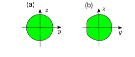
Figure 1: Cross sections of the original and perturbed cylinders. (a): the original circular cylinders for $a=0.3L$. (b): the perturbed non-circular cylinders for $a=0.3L$ and $(\delta,\eta)=(0.05,0.05)$.

The BIC S1 is a scalar $E$-polarized standing wave ($\alpha_{*}=\beta_{*}=0$). Our theory predicts that it exists continuously on a curve in the $\delta$-$\eta$ plane. This is confirmed by numerical results for $\delta\in[0,0.1]$. The BIC remains as a standing wave, i.e., $\alpha=\beta=0$, for all $\delta$. The parameter $\eta$ and the frequency $\omega$ of the BIC depend on $\delta$, and are shown in Fig. 2(a)

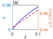
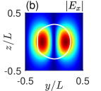
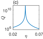
Figure 2: BIC near S1 in a perturbed array of cylinders. (a): parameter $\eta$ (solid blue curve, left axis) and frequency $\omega$ (dashed red curve, right axis) of the BIC for different values of $\delta$. (b): magnitude of the electric field (i.e. $|E_{x}|$) of the BIC for $\delta=0.05$ and $\eta=0.0440$. (c): $Q$ factor of resonant modes (with $\alpha=\beta=0$) as a function of $\eta$ for $\delta=0.05$. The peak at $\eta=0.0440$ corresponds to a BIC with $\omega=0.4467(2\pi c/L)$.

as the solid blue and dashed red curves, respectively. For $\delta=0.05$ and $\eta=0.0440$, the perturbed structure has a BIC with $\omega=0.4467(2\pi c/L)$. The magnitude of the electric field (i.e. $|E_{x}|$) of this BIC is shown in Fig. 2(b). In Fig. 2(c), we show the $Q$ factor of resonant modes (with $\alpha=\beta=0$) for fixed $\delta=0.05$ and different $\eta$.

Circularly polarized resonant states (CPSs) and BICs are polarization singularities in the momentum space (the $\alpha$-$\beta$ plane) zhen14 ; bulg17pra ; liu20 ; yoda20 . In Fig. 3,

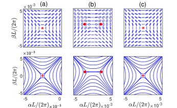
Figure 3: Emergence and annihilation of CPSs near BIC S1. (a), (b) and (c): polarization ellipses (top panels) and polarization directions (lower panels) for $(\delta,\eta)=(0,0)$, $(0.05,0)$ and $(0.05,0.0440)$, respectively. Red asterisks and dots denote BICs and CPSs, respectively.

we show polarization ellipses (upper panels) and polarization directions (lower panels) for resonant modes in periodic arrays of cylinders with (a) $\delta=\eta=0$, (b) $\delta=0.05$ and $\eta=0$, and (c) $\delta=0.05$ and $\eta=0.0440$. The resonant modes are from the band that contains BIC S1 when $\delta=\eta=0$. The BIC S1 and its extension in a perturbed array are shown as the red asterisks in panels (a) and (c), respectively. For fixed $\eta=0$ and when $\delta$ is increased, BIC S1 is destroyed and turned to a pair of CPSs with topological charge $-1/2$. The CPSs are shown as red dots in Fig. 3(b). It can be easily shown that the two CPSs must have the same $\beta$ and opposite $\alpha$. For a fixed $\delta=0.05$ and when $\eta$ is increased, the two CPSs move towards the $\beta$ axis, and form a BIC at $\eta=0.0440$ as shown in Fig. 3(c).

The BIC S2 is a scalar $E$-polarized propagating BIC. Our numerical results confirm that it can be extended to the $\delta$-$\eta$ plane on a curve, as shown in Fig. 4(a).

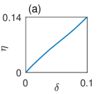
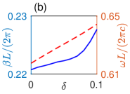
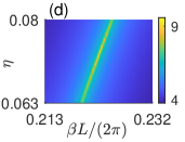
Figure 4: BIC near S2 in a perturbed array of cylinders. (a): parameter $\eta$ of the BIC as a function of $\delta$. (b): wavenumber $\beta$ (solid blue curve, left axis) and frequency $\omega$ (dashed red curve, right axis) of the BIC as functions of $\delta$. (c): magnitude of the BIC (i.e. $|{E}_{x}|$) for $\delta=0.05,\eta=0.0721$, $\alpha=0,\beta=0.2223(2\pi/L)$, and $\omega=0.6307(2\pi c/L)$. (d): logarithmic value of the $Q$ factor (i.e. $\log_{10}Q$) of resonant modes as a function of $\beta$ and $\eta$ for $\alpha=0$ and $\delta=0.05$.

The extended BIC remains scalar (i.e., $\alpha=0$) for all $\delta$. The wavenumber $\beta$ and frequency $\omega$ of this BIC (for different $\delta$) are shown in Fig. 4(b) as the solid blue and dashed red curves, respectively. For $\delta=0.05$ and $\eta=0.0721$, we obtain a BIC with $\beta=0.2223(2\pi/L)$ and $\omega=0.6307(2\pi c/L)$. The electric field magnitude (i.e. $|E_{x}|$) is shown in Fig. 4(c). In Fig. 4(d), we show the $Q$ factor of resonant modes for $\eta$ near $0.0721$ and $\beta$ near $0.2223(2\pi/L)$. In Fig. 5,

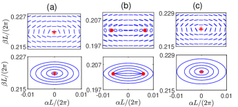
Figure 5: Emergence and annihilation of CPSs near BIC S2. (a), (b) and (c): polarization ellipses (top panels) and polarization directions (lower panels) for $(\delta,\eta)=(0,0)$, $(0.05,0)$ and $(0.05,0.0721)$, respectively.

we show polarization ellipses (upper panels) and polarization directions (lower panel) for resonant modes near the BIC and the CPSs. Keeping $\eta=0$ and increasing $\delta$ to $0.05$, the BIC S2 splits into two CPSs with topological charges $+1/2$ as shown in Fig. 5(b). Keeping $\delta=0.05$ and increasing $\eta$ to $0.0721$, the two CPSs merge and form a BIC with $\beta=0.2223(2\pi/L)$ and $\omega=0.6307(2\pi c/L)$, as shown in Fig. 5(c).

The BIC V1 is a vectorial BIC propagating along the $x$ axis. Our numerical results, shown in Fig. 6(a),

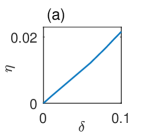
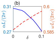
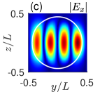
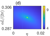
Figure 6: BIC near V1 in a perturbed array of cylinders. (a): parameter $\eta$ of the BIC as a function of $\delta$. (b): wavenumber $\alpha$ (solid blue curve, left axis) and frequency $\omega$ (dashed red curve, right axis) of the BIC as functions of $\delta$. (c): magnitude of the BIC (i.e. $|{E}_{x}|$) for $\delta=0.05$, $\eta=0.0101$, $\alpha=0.2968(2\pi/L)$, $\beta=0$, and $\omega=0.5922(2\pi c/L)$. (d): logarithmic value of the $Q$ factor (i.e. $\log_{10}Q$) of resonant modes as a function of $\eta$ and $\alpha$ for $\beta=0$ and $\delta=0.05$.

confirm that this BIC exists continuously on a curve in the $\delta$-$\eta$ plane. The wavenumber $\beta$ of this BIC remains at zero for all $\delta$. The wavenumber $\alpha$ and frequency $\omega$ are shown as functions of $\delta$ in Fig. 6(b). For $\delta=0.05$, the BIC is obtained with $\eta=0.0101$, $\alpha=0.2968(2\pi/L)$, and $\omega=0.5922(2\pi c/L)$. The magnitude of $E_{x}$ of this BIC is shown in Fig. 6(c). In Fig. 6(d), we show the $Q$ factor of resonant modes for nearby values of $\eta$ and $\alpha$ (for fixed $\delta=0.05$ and $\beta=0$). Similar to the previous examples and as shown in Fig. 7,

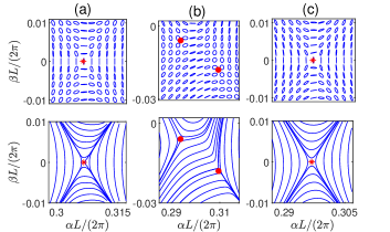
Figure 7: Emergence and annihilation of CPSs near BIC V1. (a), (b) and (c): polarization ellipses (top panels) and polarization directions (lower panels) for $(\delta,\eta)=(0,0)$, $(0.05,0)$ and $(0.05,0.0101)$, respectively.

BIC V1 splits to a pair of CPSs when $\eta$ is fixed at $0$ and $\delta$ is increased to $0.05$, and the CPSs merge to a BIC when $\delta$ is fixed at $0.05$ and $\eta$ is increased to to $0.0101$.

The BIC V2 is a vectorial BIC with both $\alpha_{*}\neq 0$ and $\beta_{*}\neq 0$. According to our theory, it can exist continuously on a curve in a 3D parameter space of $\delta$, $\eta$ and $s$. In general, we can only expect the curve to have discrete intersections with the $\delta$-$\eta$ plane. Therefore, the BIC may exist at isolated points in the plane. To find the BIC with $(\delta,\eta)\neq(0,0)$, we can vary the parameters and try to force the CPSs to merge. In Fig. 8,

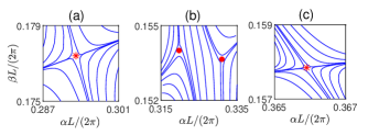
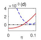
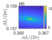
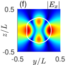
Figure 8: Emergence and annihilation of CPSs near BIC V2. (a), (b) and (c): polarization directions for $(\delta,\eta)=(0,0)$, $(0.05,0)$, and $(0.0418,0.0556)$, respectively. Red asterisks and dots denote BICs and CPSs, respectively. (d): the difference of $\alpha$ (dashed blue curve) and $\beta$ (solid red curve) of the two CPSs as functions of $\eta$ for fixed $\delta=0.05$. The unit of the vertical axis is $2\pi/L$. The horizontal dash-dot line denotes zero. (e): the logarithmic value of the $Q$ factor (i.e. $\log_{10}Q$) of nearby resonant modes as a function of $\alpha$ and $\beta$ for $(\delta,\eta)=(0.0418,0.0556)$. There is a BIC with $(\alpha,\beta)=(0.3659,0.1578)(2\pi/L)$ and $\omega=0.6303(2\pi c/L)$. (f): magnitude of the BIC (i.e. $|{E}_{x}|$).

we show the polarization directions of the nearby resonant modes and the BIC or CPSs, for $(\delta,\eta)=(0,0)$, $(0.05,0)$, and $(0.0418,0.0556)$ in panels (a), (b) and (c), respectively. For a fixed $\eta=0$ and an increasing $\delta$, BIC V2 splits to a pair of CPSs. At $\delta=0.05$ and $\eta=0$, the wavevectors of the two CPSs are $(\alpha_{1},\beta_{1})=(0.3198,0.1543)(2\pi/L)$ and $(\alpha_{2},\beta_{2})=(0.3308,0.1535)(2\pi/L)$, respectively, and are shown in Fig. 8(b) as the red dots. In Fig. 8(d), we show $\alpha_{1}-\alpha_{2}$ and $\beta_{1}-\beta_{2}$ of the two CPSs for fixed $\delta=0.05$ and different $\eta$. Since the two curves do not intersect at zero, the two CPSs do not merge (become a BIC) if $\eta$ is varied and $\delta$ is fixed at $0.05$. However, these two CPSs do merge to a BIC if $(\delta,\eta)$ is tuned to $(0.0418,0.0556)$. The wavevector of this BIC is $(\alpha,\beta)=(0.3659,0.1578)(2\pi/L)$ as shown in Fig. 8(c). Its frequency is $\omega=0.6303(2\pi c/L)$ and its topological charge is $-1$. In Fig. 8(e), we show the $Q$ factor of nearby resonant modes for $(\delta,\eta)=(0.0418,0.0556)$. The divergence of the $Q$ factor confirms the existence of this BIC. The magnitude of $E_{x}$ of this BIC is shown in Fig. 8(f).

V Conclusion

Dielectric periodic structures sandwiched between two homogeneous media are a popular platform for studying photonic BICs and their applications. We analyzed how the BICs in 2D structures with an up-down mirror symmetry and a single periodic direction depend on structural parameters, and showed that a typical vectorial BIC with nonzero wavenumber components in both invariant and periodic directions can only be found by tuning two structural parameters, while the other BICs, including the scalar ones studied in our previous work yuan20_2 , can be found by tuning one structural parameter. The theory is applicable to generic BICs with a low frequency such that there is only one radiation channel and for structures without a reflection symmetry in the periodic direction. The result is somewhat unexpected, since all these BICs exhibit the same robustness when the structure and the perturbation is symmetric in the periodic direction yuan17ol ; yuan21 . Our theory is established using an all-order perturbation method and validated by numerical examples involving periodic arrays of dielectric cylinders. The numerical studies also demonstrate the annihilation and generation of BICs and CPSs as structural parameters are varied, while the net topological charge remains unchanged.

Our study suggests that a typical BIC can exist continuously when a sufficient number of structural parameters are introduced. The number of parameters depends on the number of opening diffraction channels, the retained symmetries, and the nature of the BIC. Although our theory is developed for 2D structures with a single periodic direction, it can be extended to 3D structures with two-dimensional periodicity, and similar results are expected.

Appendix

The governing equations for vector function ${\bm{\Phi}}({\bm{r}})$ defined in Eq. (5) are

$$\left(\nabla+i{\bm{\alpha}}\right)\times\left(\nabla+i{\bm{\alpha}}\right)\times{\bm{\Phi}}-k^{2}\varepsilon({\bm{r}}){\bm{\Phi}}=0,$$ (A1)

$$\left(\nabla+i{\bm{\alpha}}\right)\cdot[\varepsilon({\bm{r}}){\bm{\Phi}}]=0,$$ (A2)

where ${\bm{\alpha}}=(\alpha,\beta,0)$. Substituting expansions (16)-(22) into Eqs. (A1) and (A2), and comparing the coefficients of $\delta^{j}$ for $j\geq 1$, we obtain Eqs. (III) and (III) for ${\bm{\Phi}}_{j}$, where

$$\mathcal{L} = (\nabla+i{\bm{\alpha}}_{*})\times(\nabla+i{\bm{\alpha}}_{*})\times\cdot-k_{*}^{2}\varepsilon({\bm{r}}),$$

$$\mathcal{B}_{n} = -i\left[(\nabla+i{\bm{\alpha}}_{*})\times{\bm{e}}_{n}\times\cdot+{\bm{e}}_{n}\times(\nabla+i{\bm{\alpha}}_{*})\times\cdot\right]$$

for $n=1$ and 2, ${\bm{e}}_{1}$ and ${\bm{e}}_{2}$ are the unit vectors in the $x$ and $y$ directions, respectively. The other scalar and vector functions in these two equations are

$$h_{1} = -i\varepsilon_{*}{\bm{e}}_{1}\cdot{\bm{\Phi}}_{*},$$

$$h_{2} = -i\varepsilon_{*}{\bm{e}}_{2}\cdot{\bm{\Phi}}_{*},$$

$$h_{3} = -(\nabla+i{\bm{\alpha}}_{*})\cdot(F{\bm{\Phi}}_{*}),$$

$$h_{4} = -(\nabla+i{\bm{\alpha}}_{*})\cdot(P{\bm{\Phi}}_{*}),$$

$$g_{j} = -\nabla\cdot(G{\bm{\Phi}}_{j-1})-iG{\bm{\alpha}}_{j-1}\cdot{\bm{\Phi}}_{*}$$

$$- i\sum_{m=1}^{j-1}(\varepsilon_{*}{\bm{\alpha}}_{m}+G{\bm{\alpha}}_{m-1})\cdot{\bm{\Phi}}_{j-m}$$

$$- i\sum_{m=1}^{j-1}(\eta_{m}F+s_{m}P){\bm{\alpha}}_{j-m}\cdot{\bm{\Phi}}_{*}$$

$$- i\sum_{m=1}^{j-1}\sum_{n=1}^{m}(\eta_{n}F+s_{n}P){\bm{\alpha}}_{m-n}\cdot{\bm{\Phi}}_{j-m},$$

$${\bm{C}}_{j} = {W}_{j}{\bm{\Phi}}_{*}+\sum_{m=1}^{j-1}({V}_{m}{\bm{\Phi}}_{j-m}+\mathcal{D}_{m}{\bm{\Phi}}_{j-m}$$

$$+{\bm{\alpha}}_{m}\times{\bm{\alpha}}_{j-m}\times{\bm{\Phi}}_{*}),$$

$${V}_{m} = W_{m}+2k_{*}k_{m}\varepsilon_{*}+k_{*}^{2}\eta_{m}F+k_{*}^{2}s_{m}P,$$

$${W}_{j} = \sum_{m=1}^{j-1}\left[k_{m}k_{j-m}\varepsilon_{*}+\sum_{l=0}^{m}k_{l}k_{m-l}(\eta_{j-m}F+s_{j}P)\right]$$

$$+\sum_{m=0}^{j-1}k_{m}k_{j-1-m}G,$$

$$\mathcal{D}_{m} = \sum_{l=1}^{m-1}{\bm{\alpha}}_{l}\times{\bm{\alpha}}_{m-l}\times\cdot$$

$$- i[(\nabla+i{\bm{\alpha}}_{*})\times{\bm{\alpha}}_{m}\times\cdot+{\bm{\alpha}}_{m}\times(\nabla+i{\bm{\alpha}}_{*})\times\cdot],$$

where ${\bm{\alpha}}_{m}=(\alpha_{m},\beta_{m},0)$, $k_{0}=k_{*}$, ${\bm{\Phi}}_{0}={\bm{\Phi}}_{*}$, ${\bm{\alpha}}_{0}={\bm{\alpha}}_{*}$, and $\eta_{0}=s_{0}=0$. More specifically, for $j=1$, we have $C_{1}=k_{*}^{2}G{\bm{\Phi}}_{*}$. Note that ${\bm{\Phi}}_{*}$ satisfies $\mathcal{L}{\bm{\Phi}}_{*}=0$.

The entries $a_{1m}$ for $m=1,2,3,4$ in the first row of coefficient matrix ${\bm{A}}$ of linear system (25) are defined as

$$a_{11} = \int_{\Omega}\overline{{\bm{\Phi}}}_{*}\cdot\mathcal{B}_{1}{\bm{\Phi}}_{*}d{\bm{r}},$$

$$a_{12} = \int_{\Omega}\overline{{\bm{\Phi}}}_{*}\cdot\mathcal{B}_{2}{\bm{\Phi}}_{*}d{\bm{r}},$$

$$a_{13} = 2k_{*}\int_{\Omega}\varepsilon_{*}({\bm{r}})\overline{{\bm{\Phi}}}_{*}\cdot{\bm{\Phi}}_{*}d{\bm{r}}=2k_{*}L^{2},$$

$$a_{14} = k_{*}^{2}\int_{\Omega}F({\bm{r}})\overline{{\bm{\Phi}}}_{*}\cdot{\bm{\Phi}}_{*}d{\bm{r}},$$

$$a_{15} = k_{*}^{2}\int_{\Omega}P({\bm{r}})\overline{{\bm{\Phi}}}_{*}\cdot{\bm{\Phi}}_{*}d{\bm{r}}.$$

The entries $a_{2m}$ and $a_{3m}$ for $m=1,2,3,4$ are defined similarly as $a_{1m}$ with $\overline{{\bm{\Phi}}}_{*}$ replaced by $\overline{{\bm{\Psi}}}_{1}$ and $\overline{{\bm{\Psi}}}_{2}$, respectively. Condition (12) implies the $(2,3)$ and $(3,3)$ entries of matrix ${\bm{A}}$ are zero, i.e. $a_{23}=a_{33}=0$. The elements in the right-hand side vector ${\bm{b}}_{j}$ of linear system (25) are

$$b_{1j} = -\int_{\Omega}\overline{{\bm{\Phi}}}_{*}\cdot{\bm{C}}_{j}d{\bm{r}},$$

$$b_{21} = -\int_{\Omega}\overline{{\bm{\Psi}}}_{1}\cdot{\bm{C}}_{j}d{\bm{r}},$$

$$b_{31} = -\int_{\Omega}\overline{{\bm{\Psi}}}_{2}\cdot{\bm{C}}_{j}d{\bm{r}}.$$

The linear system (25) is a necessary and sufficient condition for Eq. (III) to have a solution that decays to zero exponentially as $|z|\to\infty$. If ${\bm{\Phi}}_{j}$ decays to zero exponentially as $|z|\to\infty$, we take the dot product of Eq. (III) with $\overline{{\bm{\Phi}}}_{*}$, $\overline{{\bm{\Psi}}}_{1}$ and $\overline{{\bm{\Psi}}}_{2}$, respectively, integrate the results on domain $\Omega$ as in Appendix A of Ref. yuan21 , and obtain linear system (25). On the other hand, if system (25) has a real solution, the first equation in (25) ensures that Eq. (III) is solvable, and the second and third equations of (25) guarantee that the solution of Eq. (III) decays exponentially to zero as $|z|\to\infty$.

More specifically, the inhomogeneous equation (III) has a non-zero solution only if the right hand side is orthogonal to ${\bm{\Phi}}_{*}$, that is, if the first equation of linear system (25) is true. Since there is only one opening diffraction channel, the asymptotic formulae of diffraction solutions ${\bm{\Psi}}_{m}$ (for $m=1,2$) at infinity are

$${\bm{\Psi}}_{m}\sim{\bm{f}}_{m}^{\pm}e^{\pm i\gamma_{*}z}+{\bm{g}}_{m}^{\mp}e^{\mp i\gamma_{*}z},\quad z\to\mp\infty,$$

where ${\bm{g}}_{m}^{\pm}=(g_{mx},g_{my},\pm g_{mz})$ are constant vectors satisfying ${\bm{g}}_{m}^{\pm}\cdot{\bm{k}}_{*}^{\pm}=0$ for ${\bm{k}}_{*}^{\pm}=(\alpha_{*},\beta_{*},\pm\gamma_{*})$ and $\gamma_{*}=(k_{*}^{2}\varepsilon_{0}-\alpha_{*}^{2}-\beta_{*}^{2})^{1/2}$. For each $j\geq 1$, the asymptotic formula of ${\bm{\Phi}}_{j}$ at infinity is

$${\bm{\Phi}}_{j}\sim{\bm{d}}_{j}^{\pm}e^{\pm i\gamma_{*}z},\quad z\to\pm\infty,$$

where ${\bm{d}}_{j}^{\pm}=(d_{jx},d_{jy},\pm d_{jz})$ are constant vectors satisfying ${\bm{d}}_{j}^{\pm}\cdot{\bm{k}}_{*}^{\pm}=0$. To show that ${\bm{\Phi}}_{j}$ decays exponentially, we only need to show ${\bm{d}}_{j}^{+}={\bm{0}}$. Taking the dot product of Eq. (III) with $\overline{{\bm{\Psi}}}_{m}$ (for $m=1,2$), integrating the results on domain $\Omega_{h}=\left\{(x,y)||x|<h,|y|<L/2\right\}$ for $h>d$, and following the same procedure in Appendix B of yuan21 , we have

$$\lim_{h\to\infty}\int_{\Omega_{h}}\overline{{\bm{\Phi}}}_{m}\cdot\mathcal{L}{\bm{\Phi}}_{j}d{\bm{r}}=-4i\alpha L\overline{{\bm{g}}}_{m}^{+}\cdot{\bm{d}}_{j}^{+}.$$ (A3)

The second and third equations of the linear system (27) imply the left hand side in above equation is zero for $m=1,2$. Therefore, $\overline{{\bm{g}}}_{m}^{+}\cdot{\bm{d}}_{j}^{+}=0$. Since $\left\{{\bm{g}}_{1},{\bm{g}}_{2},{\bm{k}}_{*}^{+}\right\}$ is a linearly independent set, we have ${\bm{d}}_{j}^{+}={\bm{d}}_{j}^{-}={\bm{0}}$.

For a vectorial BIC with $\alpha_{*}\neq 0$ and $\beta_{*}=0$, the electric field ${\bm{E}}_{*}={\bm{\Phi}}_{*}$ and the corresponding diffraction solutions ${\bm{E}}^{(s)}_{1}={\bm{\Psi}}_{1}$ and ${\bm{E}}^{(s)}_{2}={\bm{\Psi}}_{2}$ satisfy condition (14), i.e. their $x$ components are pure imaginary and their $y$ and $z$ components are real. It is easy to show that $\mathcal{B}_{1}{\bm{\Phi}}_{*}$ also satisfies condition (14), the $x$ component of $\mathcal{B}_{2}{\bm{\Phi}}_{*}$ is real, and the $y$ and $z$ components of $\mathcal{B}_{2}{\bm{\Phi}}_{*}$ are pure imaginary. Therefore, $a_{22}$ and $a_{32}$ are pure imaginary, and all other elements of ${\bm{A}}$ are real. For $j=1$, ${\bm{C}}_{1}=k_{*}^{2}G{\bm{\Phi}}_{*}$ satisfies condition (14), $b_{11}$, $b_{12}$ and $b_{13}$ are real. If $a_{21}a_{34}-a_{24}a_{31}\neq 0$, the complex linear system (27) for $j=1$ has a real solution with $\beta_{1}=0$ and $\alpha_{1}$, $k_{1}$, $\eta_{1}$ satisfying Eq. (28). Therefore, ${\bm{\Phi}}_{1}$ can be solved from Eq. (III) for $j=1$ and it decays to zero exponentially as $|z|\to+\infty$. In addition, since the right hand side of Eq. (III) for $j=1$ satisfies Eq. (14), ${\bm{\Phi}}_{1}$ also can be scaled to satisfies Eq. (14). For any $j\geq 2$, if $\alpha_{m}$, $k_{m}$, $\eta_{m}$ are real, $\beta_{m}=0$ and ${\bm{\Phi}}_{m}$ satisfies Eq. (14) for $m<j$, then ${\bm{C}}_{j}$ satisfies Eq. (14) and $b_{1j}$, $b_{2j}$, $b_{3j}$ are real. The same reasoning can be used to show that linear system Eq. (27) has a real solution with $\beta_{j}=0$ and $\alpha_{j}$, $k_{j}$, $\eta_{j}$ satisfying Eq. (28), and ${\bm{\Phi}}_{j}$ can be solved from Eq. (III) and satisfies Eq. (14).

A scalar BIC with $\alpha_{*}=0$ and $\beta_{*}\neq 0$, is either $E$- or $H$-polarized. Without loss of generality, we assume the BIC ${\bm{E}}_{*}$ (i.e. ${\bm{\Phi}}_{*}$) is $H$-polarized. In that case, we let ${\bm{f}}_{1}=(1,0,0)$ and ${\bm{f}}_{2}$ be orthogonal to ${\bm{f}}_{1}$ and ${\bm{k}}_{*}^{+}$, then ${\bm{E}}_{1}^{(s)}$ (i.e. ${\bm{\Psi}}_{1}$) is $E$-polarized and ${\bm{E}}_{2}^{(s)}$ (i.e. ${\bm{\Psi}}_{2}$) is $H$-polarized. It is easy to show that $\mathcal{B}_{1}{\bm{\Phi}}_{*}$ is $E$-polarized and $\mathcal{B}_{2}{\bm{\Phi}}_{*}$ is $H$-polarized. Therefore, $a_{11}=a_{22}=a_{31}=a_{24}=0$. For $j=1$, ${\bm{C}}_{1}=k_{*}^{2}G{\bm{\Phi}}_{*}$ is also $H$-polarized and $b_{21}=0$. If $a_{32}\neq 0$ and $\mbox{Im}(a_{34}/a_{32})\neq 0$, then the linear system (27) for $j=1$ has a real solution with $\alpha_{1}=0$ and $\beta_{1}$, $k_{1}$, $\eta_{1}$ satisfying Eq. (29). Thus, ${\bm{\Phi}}_{1}$ can be solved from Eq. (III) for $j=1$ and ${\bm{\Phi}}_{j}\to 0$ exponentially as $|z|\to+\infty$. In addition, since the right hand side of Eq. (III) for $j=1$ is $H$-polarized, ${\bm{\Phi}}_{1}$ is also $H$-polarized. For any $j\geq 2$, if $\alpha_{m}=0$, $\beta_{m}$, $k_{m}$, $\eta_{m}$ are real and ${\bm{\Phi}}_{m}$ is $H$-polarized for $m<j$, then ${\bm{C}}_{j}$ is $H$-polarized and $b_{2j}=0$. Therefore, linear system (27) has a real solution with $\alpha_{j}=0$ and $\beta_{j}$, $k_{j}$, $\eta_{j}$ satisfying Eq. (29), and ${\bm{\Phi}}_{j}$ can be solved from Eq. (III) and is $H$-polarized.

References

- (1) C. W. Hsu, B. Zhen, A. D. Stone, J. D. Joannopoulos, and M. Soljačić, “Bound states in the continuum,” Nat. Rev. Mater. 1, 16048 (2016).
- (2) K. Koshelev, G. Favraud, A. Bogdanov, Y. Kivshar, and A. Fratalocchi, “Nonradiating photonics with resonant dielectric nanostructures,” Nanophotonics 8, 725–745 (2019).
- (3) S. I. Azzam and A. V. Kildishev, “Photonic bound states in the continuum: from basics to applications,” Adv. Opt. Mater. 9, 2001469 (2021).
- (4) A.-S. Bonnet-Bendhia and F. Starling, “Guided waves by electromagnetic gratings and nonuniqueness examples for the diffraction problem,” Math. Methods Appl. Sci. 17, 305-338 (1994).
- (5) R. Porter and D. Evans, “Embedded Rayleigh-Bloch surface waves along periodic rectangular arrays,” Wave Motion 43, 29-50 (2005).
- (6) D. C. Marinica, A. G. Borisov, and S. V. Shabanov, “Bound states in the continuum in photonics,” Phys. Rev. Lett. 100, 183902 (2008).
- (7) Y. Plotnik, O. Peleg, F. Dreisow, M. Heinrich, S. Nolte, A. Szameit, and M. Segev, “Experimental observation of optical bound states in the continuum,” Phys. Rev. Lett. 107, 183901 (2011).
- (8) C. W. Hsu, B. Zhen, J. Lee, S.-L. Chua, S. G. Johnson, J. D. Joannopoulos, and M. Soljačić, “Observation of trapped light within the radiation continuum,” Nature 499, 188–191 (2013).
- (9) E. N. Bulgakov and A. F. Sadreev, “ Bloch bound states in the radiation continuum in a periodic array of dielectric rods,” Phys. Rev. A 90, 053801 (2014).
- (10) C.-L. Zou, J.-M. Cui, F.-W. Sun, X. Xiong, X.-B. Zou, Z.- F. Han, and G.-C. Guo, “Guiding light through optical bound states in the continuum for ultrahigh- microresonantors,” Laser Photonics Rev. 9, 114-119 (2015).
- (11) J. Gomis-Bresco, D. Artigas, and L. Torner, “Anisotropy-induced photonic bound states in the continuum,” Nature Photonics 11, 232–237 (2017).
- (12) K. Koshelev, S. Lepeshov, M. Liu, A. Bogdanov, and Y. Kivshar, “Asymmetric metasurfaces with high- resonances governed by bound states in the contonuum,” Phys. Rev. Lett. 121, 193903 (2018).
- (13) Z. Hu and Y. Y. Lu, “Resonances and bound states in the continuum on periodic arrays of slightly noncircular cylinders,” J. Phys. B: At. Mol. Opt. Phys. 51, 035402 (2018).
- (14) L. Yuan and Y. Y. Lu, “Perturbation theories for symmetry-protected bound states in the continuum on two-dimensional periodic structures,” Phys. Rev. A 101, 043827 (2020).
- (15) A. Taghizadeh and I.-S. Chung, “Quasi bound states in the continuum with few unit cells of photonic crystal slab,” Appl. Phys. Lett. 111, 031114 (2017).
- (16) M. V. Rybin, K. L. Koshelev, Z. F. Sadrieva, K. B. Samusev, A. A. Bogdanov, M. F. Limonov, and Y. S. Kivshar, “High- Supercavity Modes in Subwavelength Dielectric Resonators”, Phys. Rev. Lett. 119, 243901 (2017).
- (17) Z. Hu, L. Yuan, and Y. Y. Lu, “Bound states with complex frequencies near the continuum on lossy periodic structures,” Phys. Rev. A 101, 013906 (2020).
- (18) L. Yuan and Y. Y. Lu, “Bound states in the continuum on periodic structures surrounded by strong resonances,” Phys. Rev. A 97, 043828 (2018).
- (19) J. Jin, X. Yin, L. Ni, M. Soljacic, B. Zhen, and C. Peng, “Topologically enable unltra-high- guided resonances robust to out-of-plane scattering,” Nature 574, 501-504 (2019).
- (20) Z. Hu, L. Yuan, and Y. Y. Lu, “Resonant field enhancement near bound states in the continuum on periodic structures,” Phys. Rev. A 101, 043825 (2020).
- (21) A. Kodigala, T. Lepetit, Q. Gu, B. Bahari, Y. Fainman, and B. Kanté, “Lasing action from photonic bound states in continuum,” Nature 541, 196-199 (2017).
- (22) F. Yesilkoy, E. R. Arvelo, Y. Jahani, M. Liu, A. Tittl, V. Cevher, Y. Kivshar, and H. Altug, “Ultrasensitive hyperspectral imaging and biodetection enabled by dielectric metasurfaces,” Nature Photonics 13, 390-396 (2019).
- (23) K. Koshelev, S. Kruk, E. Melik-Gaykazyan J.-H. Choi, A. Bogdanov, H.-G. Park, Y. Kivshar, “Subwavelength dielectric resonators for nonlinear nanophotonics,” Science 367, 288-292 (2020).
- (24) Z. Yu, X. Xi, J. Ma, H. K. Tsang, C.-L. Zou, and X. Sun, “Photonic integrated circuits with bound states in the continuum,” Optica 6, 1342-1348 (2019).
- (25) B. Zhen, C. W. Hsu, L. Lu, A. D. Stone, and M. Soljačič, “Topological nature of optical bound states in the continuum,” Phys. Rev. Lett. 113, 257401 (2014).
- (26) E. N. Bulgakov and D. N. Maksimov, “Bound states in the continuum and polarization singularities in periodic arrays of dielectric rods,” Phys. Rev. A 96, 063833 (2017).
- (27) W. Liu, B. Wang, Y. Zhang, J. Wang, M. Zhao, F. Guan, X. Liu, L. Shi, and J. Zi, “Circularly Polarized States Spawning from Bound States in the Continuum,” Phys. Rev. Lett. 123, 116104 (2019).
- (28) T. Yoda and M. Notomi, “Generation and annihilation of topologically protected bound states in the continuum and circularly polarized states by symmetry breaking,” Phys. Rev. Lett. 125, 053902 (2020).
- (29) A. Abdrabou and Y. Y. Lu, “Circularly polarized states and propagating bound states in the continuum in a periodic array of cylinders,” Phys. Rev. A 103, 043512 (2021).
- (30) P. Paddon and J. F. Young, “Two-dimensional vector-coupled-mode theory for textured planar waveguides,” Phys. Rev. B 61, 2090-2101 (2000).
- (31) T. Ochiai and K. Sakoda, “Dispersion relation and optical transmittance of a hexagonal photonic crystal slab,” Phys. Rev. B 63, 125107 (2001).
- (32) S. G. Tikhodeev, A. L. Yablonskii, E. A Muljarov, N. A. Gippius, and T. Ishihara, “Quasi-guided modes and optical properties of photonic crystal slabs,” Phys. Rev. B 66, 045102 (2002).
- (33) S. P. Shipman and S. Venakides, “Resonance and bound states in photonic crystal slabs,” SIAM J. Appl. Math. 64, 322-342 (2003).
- (34) J. Lee, B. Zhen, S. L. Chua, W. Qiu, J. D. Joannopoulos, M. Soljačić, and O. Shapira, “Observation and differentiation of unique high-Q optical resonances near zero wave vector in macroscopic photonic crystal slabs,” Phys. Rev. Lett. 109, 067401 (2012).
- (35) Y. Yang, C. Peng, Y. Liang, Z. Li, and S. Noda, “Analytical perspective for bound states in the continuum in photonic crystal slabs,” Phys. Rev. Lett. 113, 037401 (2014).
- (36) R. Gansch, S. Kalchmair, P. Genevet, T. Zederbauer, H. Detz, A. M. Andrews, W. Schrenk, F. Capasso, M. Lončar, and G. Strasser, “Measurement of bound states in the continuum by a detector embedded in a photonic crystal,” Light: Science & Applications 5, e16147 (2016).
- (37) L. Yuan and Y. Y. Lu, “Bound states in the continuum on periodic structures: perturbation theory and robustness,” Opt. Lett. 42(21), 4490-4493 (2017).
- (38) L. Yuan and Y. Y. Lu, “Conditional robustness of propagating bound states in the continuum in structures with two-dimensional periodicity,” Phys. Rev. A 103, 043507 (2021).
- (39) L. Yuan and Y. Y. Lu, “Parametric dependence of bound states in the continuum on periodic structures,” Phys. Rev. A 102, 033513 (2020).